Estimation of Base Flow by Optimal Hydrograph Separation for the Conterminous United States and Implications for National-Extent Hydrologic Models

Abstract

Optimal hydrograph separation (OHS) uses a two-parameter recursive digital filter that applies specific conductance mass-balance constraints to estimate the base flow contribution to total streamflow at stream gages where discharge and specific conductance are measured. OHS was applied to U.S. Geological Survey (USGS) stream gages across the conterminous United States to examine the range/distribution of base flow inputs and the utility of this method to build a hydrologic model calibration dataset. OHS models with acceptable goodness-of-fit criteria were insensitive to drainage area, stream density, watershed slope, elevation, agricultural or perennial snow/ice land cover, average annual precipitation, runoff, or evapotranspiration, implying that OHS results are a viable calibration dataset applicable in diverse watersheds. OHS-estimated base flow contribution was compared to base flow-like model components from the USGS National Hydrologic Model Infrastructure run with the Precipitation-Runoff Modeling System (NHM-PRMS). The NHM-PRMS variable gwres_flow is most conceptually like a base flow component of streamflow but the gwres_flow contribution to total streamflow is generally smaller than the OHS-estimated base flow contribution. The NHM-PRMS variable slow_flow, added to gwres_flow, produced similar or greater estimates of base flow contributions to total streamflow than the OHS-estimated base flow contribution but was dependent on the total flow magnitude.

1. Introduction

Base flow is water that sustains a stream or river when no immediate precipitation has occurred and can be thought of as a mixture of different groundwater contributions that may include water from unsaturated soil reservoirs [1,2]. This critical component of streamflow is important for sustaining surface water quantity and quality during low flows, drier months of the year, or during periods of drought [3,4,5,6,7,8,9]. Quantification of the base flow across the nation is important for assessing the long-term effects of climatic, landscape, and anthropogenic influences on water quantity and stream ecosystem health [10,11,12], in addition to providing critical validation and calibration information for national-extent models [13,14]. The hydrograph separation techniques described in this study were applied to estimate base flow across the conterminous United States (CONUS) and are valuable in providing validation or calibration data for national-extent hydrologic models, further improving our capacity for understanding and predicting hydrologic conditions for the nation.

Base flow is generally not measured directly but is estimated using a variety of methods, including hydrograph separation. Hydrograph separation techniques comprise dividing a hydrograph into two or more components that represent multiple sources of flow using a priori determined criteria to justify the division [2,15]. Hydrograph separation is a common way to estimate base flow, as the various methods are inexpensive and easily implemented using stream discharge and chemistry data. Many base flow estimation methods employ graphical hydrograph separation techniques or recession analysis to infer base flow contributions, but these methods are subjective when performed manually, have no physical basis, and have no means of determining the accuracy of the estimates [16,17,18]. Automated approaches to graphical hydrograph separation are more objective and reproducible than previous manual methods, but still maintain similar caveats with regards to physical ground-truthing and accuracy [19]. This inaccuracy is because the recession curve, or the falling limb of a hydrograph, is theoretically related to groundwater storage depletion and flow to a stream. Limitations with regards to physical basin characteristics, such as drainage area and basin relief, have also restricted where purely graphical hydrograph methods were applicable [20,21,22]. This is because relatively large basins (>1300 km²) can have nonuniform rainfall and storm events, and there can be more heterogeneity in riparian storage that may affect how quickly flow and base flow are separated [20,21,22]. Despite these limitations, graphical hydrograph separation is still heavily used because of the modest data requirements.

Alternatively, hydrograph separation based on tracer-chemical mass balance methods is considered to have more of a physical basis than purely graphical separation methods because they incorporate hydrogeochemical information of the stream and hydrogeochemical discharge relationships can be inferred to define representations of base flow and quick flow [23,24,25,26,27]. In addition, accuracy can be examined from comparisons of observed and simulated stream chemistry resulting from chemical mass balance methods. Tracer-chemical mass balance hydrograph separation techniques are also not as restricted as graphical methods in terms of basin size due to assumptions of mass balance, as these techniques have been used on basins larger than 60,000 km² [25]. Most chemical mass balance methods assume that a base flow signal consists of a more concentrated chemical or solute signature than quick flow because base flow has a longer residence time, allowing for greater weathering of bedrock and soil in the subsurface. This subsurface flow, laden with weathering products of cations and anions, is eventually delivered to the stream and can be separated from quick flow based on this solute-laden signature. In streams where chemical constituents may not change as expected with changing discharge, such as in environments with the presence of volcanics or carbonates, chemical mass balance methods may be challenging to use [28,29].

In this study, we estimated base flow contributions to streamflow throughout the CONUS by employing an alternative hydrograph separation method to traditional graphical and purely tracer-chemical based methods called optimal hydrograph separation (OHS) [30,31]. OHS is unique in that in addition to being automated and reproducible, the method produces estimates of model accuracy and is objective in choosing acceptable models because of its reliance on optimization methods. OHS has similar assumptions of discharge–chemistry relationships as tracer-chemical mass balance methods and has a basis in the linear reservoir theory for groundwater as provided by the inclusion of a recursive digital filter [32]. The goals of this study were to (1) apply OHS methodology at stream gages distributed across the CONUS and evaluate patterns in OHS-derived base flow, and (2) evaluate the similarities of observation-based OHS base flow estimates to simulated National Hydrologic Model-Precipitation Runoff Modeling System (NHM-PRMS) base-flow-analogous components [13,14]. The PRMS [33] is a deterministic distributed-parameter physical-process-based modeling system developed to evaluate the response of various combinations of climate and land uses on streamflow and general watershed hydrology.

2. Materials and Methods

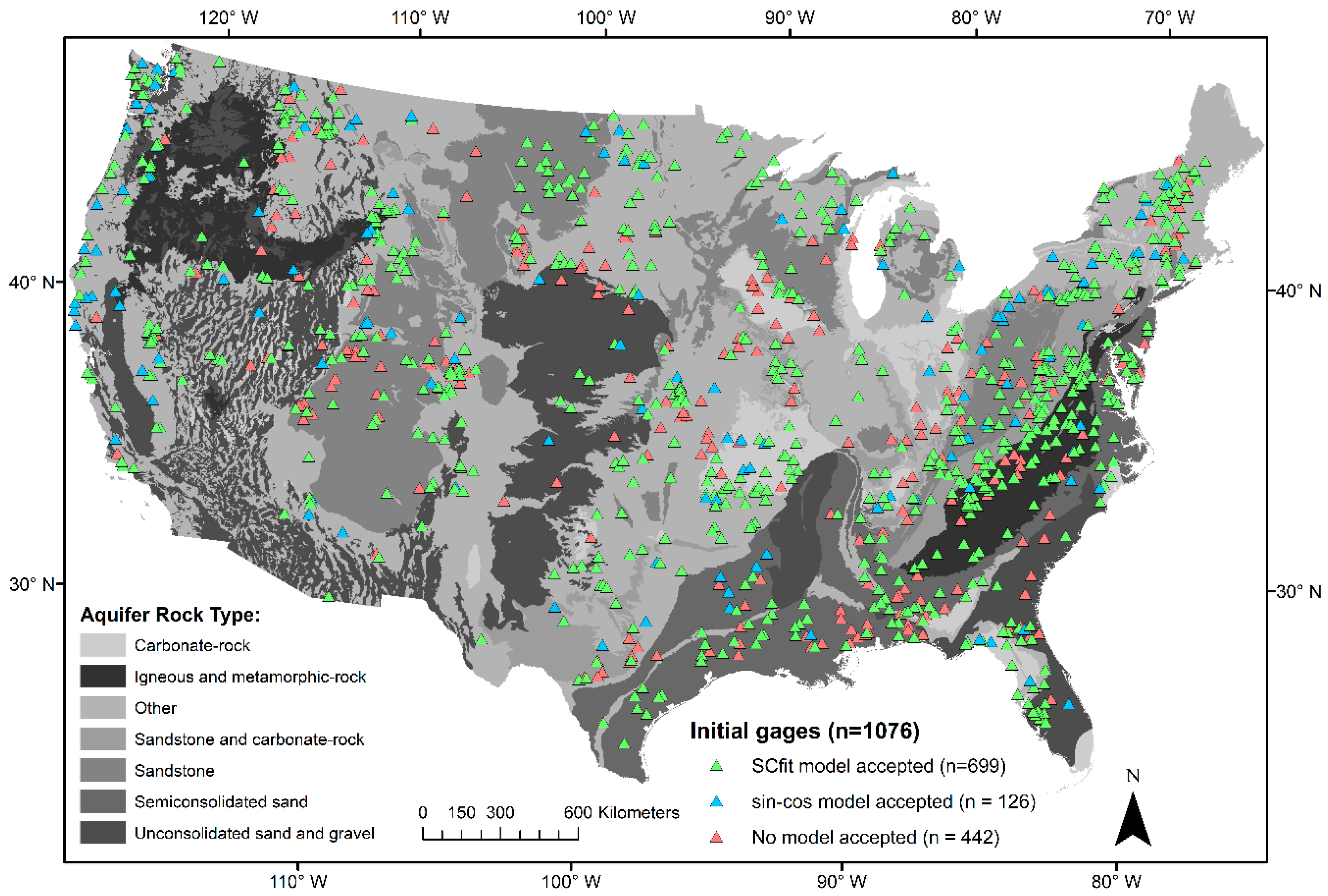
2.1. Site Selection

The study sites were chosen based on data availability in the form of spatial and temporal coverage of specific conductance and daily streamflow data within the CONUS (Figure 1).

Stream gages were initially selected from the Geospatial Attributes of Gages for Evaluating Streamflow (GAGES-II) reference stream gage dataset [34]. Gages were selected if the gage had at least three measurements of daily mean stream discharge accompanied by either a simultaneous daily mean specific conductance or an individual water quality specific conductance measurement, and where a peak in specific conductance could be detected. This resulted in 1076 stream gages to initially investigate. The data used in this study are available from the U.S. Geological Survey (USGS) National Water Information System (NWIS) database [35]. The study locations strictly used in the OHS application consisted of any available time periods in NWIS. OHS and NHM-PRMS comparison sites were selected if study locations had data after water year (WY) 1983, where a water year starts on 1 October of the previous year and ends 30 September of the year that is designated as the water year.

2.2. Optimal Hydrograph Separation

Two-component hydrograph separation, separation of base flow from quick flow, for the chosen sites was performed via OHS using a recursive digital filter (RDF) constrained by specific conductance mass balance [30,31]. An RDF is a technique used in hydrograph separation in which a digital filter is used to differentiate between low-frequency and high-frequency discharge data [19,32]. One assumption is that high-frequency discharge data are associated with direct flow or quick flow from storms or snowmelt, whereas low-frequency discharge is associated with slow flow or base flow, as discharge is less likely to change erratically. The physical basis for the RDF is the assumption that the output from an aquifer is linearly proportional to its storage (linear reservoir), which may not be valid in all settings. However, digital filters are a vital component in hydrograph separation because the methods are objective and reproducible. In this study, we used a general two-parameter RDF proposed by Eckhardt [32],

$$Q_{B_j}=\frac{\left[\left(1-\beta \right)\alpha Q_{B_{j-1}}+\left(1-\alpha \right)\beta Q_j\right]}{\left(1-\alpha \beta \right)},$$

(1)

where the first parameter, α (dimensionless), is the recession constant, the second parameter, β (dimensionless), is defined as the maximum value of the base flow index (BFImax, as defined by Eckhardt [32]), Q_B is the base flow discharge (L³ t⁻¹), Q is the total streamflow (L³ t⁻¹), and j represents the jth timestep in days.

Recession constant parameters, α, were derived for each study site from NHM-PRMS groundwater flow coefficients (gwflow_coef) (t⁻¹). Initial groundwater flow coefficients for the NHM-PRMS were generated using a multiple-linear regression equation relating BFI, drainage density, geology, vegetation type, and aquifer type [13], where BFI information was based on USGS HYSEP base flow separation applied to stream gages within the GAGES-II dataset [34,36]. Typically, α was calculated via recession analysis on recession curves of a hydrograph; programs such as RECESS (USGS) automate this process [18,20,21,37]. For each Hydrologic Response Unit (HRU), the initial gwflow_coef values could vary +/− 10% to produce the final gwflow_coef values used in this study [37]. The parameters, gwflow_coef and α, both describe watershed hydrologic response; however, gwflow_coef represents the outflow rate from a HRU amid timesteps (fraction/day), whereas α describes a base flow decay rate that can be thought of as the rate of volumetric storage depletion between timesteps. Groundwater flow coefficients, originally developed for individual HRUs, are an area-weighted average of all HRUs within each study watershed and related to α via

$$\alpha =e^{\left(-gwflow\_coef\times d\left(t\right)\right)}.$$

(2)

The recession constant parameter was temporally fixed for each watershed over the duration of the data record, and ranged from 0.936 to 0.998 for the initial 1076 chosen site locations.

The second adjustable parameter in the two-parameter RDF, β, is a fitted, unmeasurable parameter that ranges from 0 to 1 [30,32]. β is optimized using specific conductance data and mass-balance techniques [31]. Streamflow is initially separated into two components, base flow (Q_B) and quick flow (Q_S), while values of specific conductance are proposed for the base flow (C_B) and quick flow (C_S) components. These variables, as well as streamflow (Q), are used to estimate stream specific conductance (C_sep) via,

$$C_{se{p}_j}=\frac{C_B{Q}_{B_j}\left(\beta \right)+C_S{Q}_{S_j}\left(\beta \right)}{Q_j}.$$

(3)

The root-mean-squared-error, E between the estimated stream specific conductance and observed stream specific conductance (C_obs) is calculated as

$$E\left(\beta \right)={\left[{\displaystyle \sum }_{j=1}^{j=n}{\left[C_{ob{s}_j}-C_{se{p}_j}\left(\beta \right)\right]}^2\right]}^{1/2}.$$

(4)

This process is repeated until there is minimized error, E, implying that the parameter value for β is also optimized [31]. Optimization was performed in R version 3.4.3 (A Language and Environment for Statistical Computing) [38] using the algorithm “Bound Optimization by Quadratic Approximation” (BOBYQA) in the R package nloptr: The NLopt nonlinear-optimization package version 1.0.4 [39,40].

Two OHS models were used to estimate base flow specific conductance (C_B) [30]. The first OHS model estimated specific conductance via a sine-cosine function over time (sin-cos model) to emulate seasonal variation and is defined as

$$C_{B_j}=C_B+C_B{}^{*s}\left[sin\left(\frac{2\pi \left(t_j-t_0\right)}{365.25}\right)\right]+C_B{}^{*c}\left[cos\left(\frac{2\pi \left(t_j-t_0\right)}{365.25}\right)\right],$$

(5)

where $t_j$ represents the time/day of interest, $t_0$ is the beginning time/day, $C_B$ is the mean base flow specific conductance value, and $C_B{}^{*s}$ and $C_B{}^{*c}$ are amplitudes. With this model, six variables are optimized through Equations (3)–(5): β, $C_S$, $C_B$, $C_B{}^{*s}$, $C_B{}^{*c}$, and $t_0$.

The second OHS model estimates $C_B$ by using a peak-identification algorithm and linear interpolation (SCfit model). One main assumption is that greater stream specific conductance is associated with a greater base flow fraction, not necessarily the volume of total flow delivery to a stream. This assumption therefore ignores (or incorporates as base flow) high conductivity runoff from intense rain events and influences from road salt [30]. Therefore, peaks in the observed specific conductance data were identified using the function findpeaks in the R package pracma: Practical Numerical Math Functions [41], while $C_B$ values were estimated with linear interpolation between the identified peaks. The SCfit model has only two variables to optimize (β, $C_B$). SCfit and sin-cos models were accepted if the Nash-Sutcliffe efficiency coefficient (NSE) was greater than 0.3 and β did not converge to a user-defined optimization bound (lower bound = 0.00001; upper bound = 1.0) [30,42]. The NSE cutoff value of 0.3 is the same as that used in Raffensperger et al. (2017) [30].

The two parameters (α, β) and output data from OHS (long-term base flow index (BFI), the fraction of days with streamflow equal to base flow (BF Days), were examined for model type and acceptance behavior among various watershed characteristics compiled in the GAGESII dataset: drainage area, mean watershed slope, stream density, mean-annual potential evapotranspiration, mean-annual precipitation, annual runoff, percent of snow to total precipitation, and percent land cover designated as agriculture [34]. The chosen watershed characteristics were hypothesized and previously noted to be relevant in base flow delivery to rivers and streams [43].

2.3. NHM-PRMS

The National Hydrologic Model infrastructure used with the Precipitation-Runoff Modeling System (NHM-PRMS) is a physically based daily timestep hydrologic model that simulates components of the hydrologic cycle for 109,951 HRUs across the CONUS [13,14,33,44,45]. The NHM infrastructure consists of three components: (1) a physical model code, (2) climate input datasets, and (3) the spatially distributed modeling units and parameters (Geospatial Fabric).

The structure of HRUs and stream segments in NHM-PRMS is the Geospatial Fabric (GF) for National Hydrologic Modeling [46], which was aggregated from the National Hydrography Dataset, NHDPlusV1 [47]. The GF provides a consistent structure for indexing distributed parameter sets, as used by NHM-PRMS. A default set of parameters for NHM-PRMS CONUS-extent simulations was derived from consistent methodologies for every HRU and stream segment in the GF [13,48,49]. The GF also indexes stream segments and HRUs to an associated USGS stream gage of interest, allowing model parameters and simulation output variables to be easily extracted using the Bandit software [13]. The NHM-PRMS has several limitations and, like many hydrologic models and OHS, has a linearity assumption for the groundwater reservoir. Another key limitation is the static input parameters (such as the soil permeability and gwflow_coef) that control the flow into and out of subsurface reservoirs. However, recent developments to PRMS have incorporated dynamic parameters for several parts of the water cycle [50,51]. These static or dynamic parameters are spatially distributed throughout the CONUS, but their application is dependent on the GF discretization and size of HRUs, and thus, may not represent smaller-scale values.

The default parameters for NHM-PRMS [48] were calibrated for each HRU using CONUS-extent data sets of water cycle components, referred to as the “byHRU” calibration [51,52]. In this calibration procedure, the underlying calibration scheme of the Shuffled Complex Evolution method was used [53,54,55], which determined optimal parameter sets by minimizing the error between NHM-PRMS-simulated water budget components and each CONUS-extent water cycle component. This paper uses model output from an application of the NHM-PRMS with the byHRU calibration [37] using the Daymet version 3 air temperature and precipitation forcings [56].

The NHM-PRMS output variables thought to best represent conceptual base flow and streamflow from the byHRU model simulation were summarized by watershed where model HRUs and stream segments corresponded to GAGES-II reference gages. Ninety-eight sites were removed from this study because their drainage area from the NHM-PRMS GF differed by more than 10% of the reported NWIS/GAGES-II drainage area, an artifact of the original GF delineation process. In the NHM-PRMS, two variables are most analogous to base flow. The first variable, gwres_flow (GWF), conceptually represents groundwater discharge from the NHM-PRMS groundwater reservoir. The second variable, slow_flow (SF), conceptually represents the slow interflow from the NHM-PRMS gravity reservoir (soil reservoir). We hypothesized that base flow would be conceptually equivalent to GWF and/or to the combination of GWF + SF (GWFSF) for comparison with the OHS estimated base flow in this study. Total flow is conceptually represented by the output variable seg_outflow for the watershed segment indexed to the GAGES-II stream gage. The base flow fraction of total streamflow is calculated as the percent contribution of GWF or GWFSF to seg_outflow in each watershed. This approach combines HRU-based depth estimates (GWF, SF), components that lack route-timing, with routed-based daily flow estimates (seg_outflow), which incorporates watershed in-stream storage. This may lead to instances where GWFSF is greater than the outflow from an NHM-PRMS basin, especially in regions where there is more depression storage and greater in-stream storage. It is also important to acknowledge that NHM-PRMS components of GWF and SF only account for HRUs within the watershed boundary and do not account for groundwater divide shifts or trans-lateral subsurface flow from watershed to watershed, which are more commonly acknowledged in lower-sloped watersheds.

Model output from the byHRU-calibrated NHM-PRMS simulation is available from WY 1980 to WY 2016; nevertheless, output data from WY 1983 to WY 2016 were summarized to account for model spin-up time to reach equilibrium beyond initial conditions [37]. The variables GWF and SF were output by the NHM-PRMS as daily depth units by HRU. These depths were converted to daily flow volumes based on HRU drainage area and summed for all HRUs in each study watershed. The variable seg_outflow was exported as daily flow in a volume per time unit. Daily data were aggregated to monthly and water year flow volumes to account for the transit time between upstream HRUs/segments, and the watershed outlet stream segment, which are not always comparable at the daily time scale because of in-stream storage. We assumed that averaging on a monthly and annual timestep relieved most issues with routing and in-stream storage that would occur by mixing HRU-based depth estimates with routed-based daily flow estimates. Memory of flow components contributing to total streamflow from upstream to downstream segments (routing) is not accounted for in the byHRU-calibrated application of the NHM-PRMS.

2.4. Comparison of OHS and NHM-PRMS Base Flow

The results from OHS and byHRU-calibrated application of the NHM-PRMS were compared at monthly and annual time scales for WY 1983 to WY 2016. Some streamgage sites contain data gaps in the OHS output where NWIS daily discharge was missing, often attributed to equipment malfunction or sites that only operated seasonally. These data gaps were removed from the NHM-PRMS output record for purposes of comparison. Periods of zero flow were also removed as they are not well represented in the currently available configuration of the NHM-PRMS and are a known limitation of the byHRU calibration simulated streamflow output. OHS daily values were aggregated to monthly values for months that had a complete daily value record. Similarly, OHS monthly values were aggregated to annual values for water years that had complete monthly values.

Comparisons between the OHS base flow and byHRU-calibrated application of the NHM-PRMS components representing base flow were carried out by examination of long-term averages and averaging the difference between OHS and NHM-PRMS component percent contribution to total flow at monthly and annual time scales. We assume that GWF and GWFSF components within the NHM-PRMS best represent base flow conceptually, as there are no other subsurface components in the hydrologic model that would be analogous. Therefore, we acknowledge that we are comparing two conceptualizations of base flow (GWF, GWFSF) provided by the NHM-PRMS to an estimation of base flow provided by the OHS. The average difference between GWF and OHS base flow percent contribution to total flow (case 1) and GWFSF and OHS base flow percent contribution to total flow (case 2) is calculated as

$$\mathrm{case}1=\left(\frac{\mathrm{GWF}}{\mathrm{seg}\_\mathrm{outflow}}-\frac{\mathrm{OHS}\mathrm{base}\mathrm{flow}}{\mathrm{observed}\mathrm{streamflow}}\right)\times 100,$$

(6)

$$\mathrm{case}2=\left(\frac{\mathrm{GWFSF}}{\mathrm{seg}\_\mathrm{outflow}}-\frac{\mathrm{OHS}\mathrm{base}\mathrm{flow}}{\mathrm{observed}\mathrm{streamflow}}\right)\times 100.$$

(7)

These comparisons evaluate how well the byHRU-calibrated application of NHM-PRMS represents base flow and highlight potential improvements for OHS and NHM-PRMS. The standard difference between NHM-PRMS and OHS estimated base flow contributions were separated by normalized monthly flow quartiles and examined across watersheds within the same aquifer rock type [57] and aggregated ecoregions [34,58]. This temporal and spatial comparison provides insight into where across the CONUS and at what flow quartiles a future model calibration can use OHS results to better represent base flow in the NHM-PRMS.

3. Results

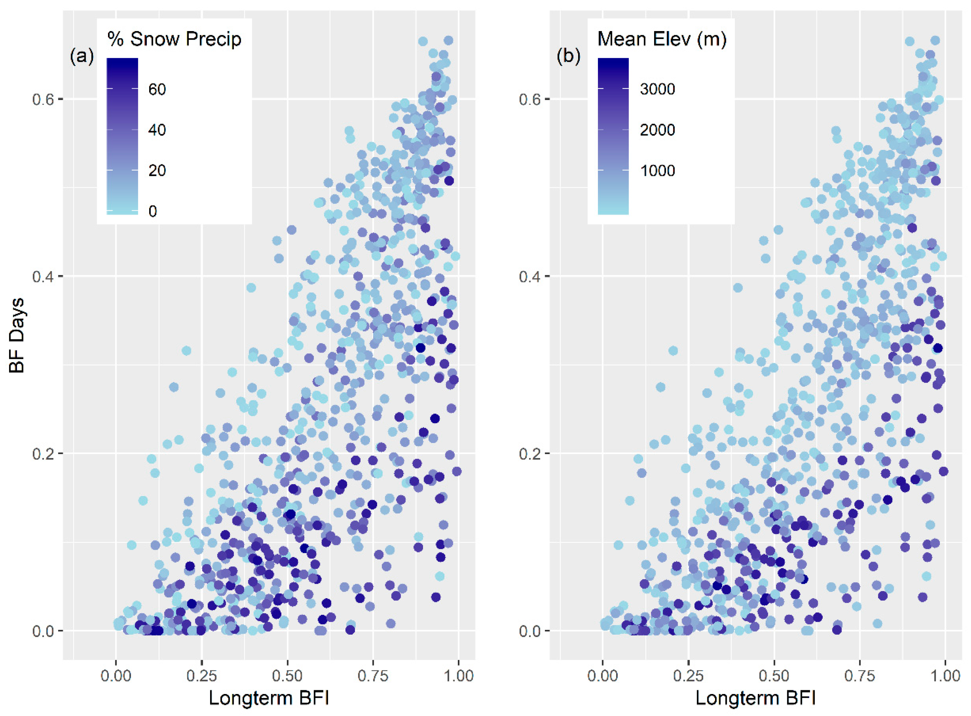
3.1. OHS Output: General Overview

Of the 1076 study stream gages that met the initial site selection criteria, most of the sites (825) have at least one OHS model type that yields an “acceptable” model. Of the 825 sites, 33 sites have only an accepted sin-cos model, 349 sites have only an accepted SCfit model, and 443 sites have acceptable sin-cos and SCfit model types. Of the 443 sites with two acceptable models, 350 sites have a greater NSE among the SCfit models and 93 have a greater NSE among the sin-cos models. In total, 699 sites have better fitting SCfit models and 126 sites have better fitting sin-cos models. Of the final 825 accepted models, the average NSE between the observed and simulated stream specific conductance is 0.62 and the overall long-term average BFI for all the study sites is 0.61 (

Table 1. Minimum, maximum, and mean values for accepted model parameters and output.

Parameter/Output	Minimum	Maximum	Mean
α	0.94	1.00	0.98
β	0.01	1.00	0.72
BFI (fraction)	0.01	0.99	0.61
BF Days (fraction)	0.00	0.67	0.26

). The largest differences between the SCfit models and sin-cos models are in the mean values of β, BFI, and BF Days (

Table 2. Minimum, maximum, and mean values for accepted model parameters, output, and metrics separated by model type (SCfit or sin-cos).

Parameter/Metric/Output	SCfit (699 Models)			sin-cos (126 Models)
	Minimum	Maximum	Mean	Minimum	Maximum	Mean
α	0.94	1.00	0.98	0.94	1.00	0.98
β	0.01	1.00	0.75	0.01	1.00	0.58
NSE	0.30	1.00	0.62	0.30	1.00	0.65
Mean Daily Streamflow (m3 s−1)	0.02	246	7.81	0.01	76.0	6.39
BFI (fraction)	0.01	0.99	0.64	0.01	0.98	0.47
BF Days (fraction)	0.00	0.67	0.28	0.00	0.66	0.18

).

Values of α are not optimized but are similar between the two models and consistent with the NHM-PRMS model [13]. β values are generally larger for SCfit models. As a result, both BFI and BF Days are generally greater for SCfit model sites. The range of β values for the CONUS is larger than was reported for Chesapeake Bay Watershed (0.26–0.92) [30], although the mean values are similar (0.61 for Chesapeake Bay Watershed and 0.72 for the CONUS).

Ranges of α, β, BFI, and BF Days for selected watershed physical and hydro-climatological characteristics were similar between SCfit and sin-cos model types (

Table 3. Minimum, maximum, and mean values for landscape and hydro-climatological features for accepted models.

Hydroclimatological Features	SCfit (699 Models)			sin-cos (126 Models)
	Min	Max	Mean	Min	Max	Mean
Watershed area, km2	1.6	14,300	779	12.3	6020	511
Mean watershed slope *, %	0.0	54.2	13.0	0.0	51.9	13.8
Percent of watershed in irrigated agriculture **, %	0.0	20.2	0.7	0.0	16.2	0.6
Watershed percent perennial ice/snow (class 12) **+, %	0.0	53.6	4.0	0.0	4.3	0.6
Mean annual precipitation for the watershed ***, cm	32.6	452	112	43.3	362	113
Snow percent of total precipitation ++, %	0.0	73.1	20.7	0.0	71.2	21.8
Mean-annual potential evapotranspiration +++, mm/year	306	1190	682	355	1150	661
Estimated watershed annual runoff +*+, mm/year	2.1	3730	435	0.0	3330	471
Stream density, km/km2 +**	0.0	1.5	0.8	0.2	1.4	0.7

* Derived from 100m resolution National Elevation Dataset; ** From USGS 2002 250-m MODIS data; **⁺ Only presented for watersheds with >0% perennial ice/snow cover (n = 55 for SCfit models, n = 126 for sin-cos); *** From 800 m PRISM data, 30 year period from 1971–2000; ⁺⁺ Mean period from 1901–2000; ⁺⁺⁺ Estimated from Hamon (1961); ⁺*⁺ Mean period from 1971–2000, estimation method integrated effects of climate, land use, water use, and regulation; ⁺** From NHD 1:100,000 streams; All watershed characteristics originally compiled within the GAGES-II dataset [34].

, Figures S1–S5), but do not display patterns with respect to watershed area (Figure 2) or stream density (Figure S1).

Values of α generally increase with increasing mean watershed slope and the percent of total precipitation composed of snow and decrease with increasing mean-annual potential evapotranspiration (PET) (Figure S2). These patterns are likely related to the method used to estimate α values based on a regression against watershed characteristics [13]. β does not display a pattern or bias with any of these watershed characteristics (Figure S3), or with estimated annual runoff, mean-annual precipitation, mean-annual PET, or percent of irrigated agriculture or perennial ice/snow land cover in a watershed for either model type (Figures S4 and S5). In general, the model output (BFI and BF Days) appears more dependent on β than α, which is potentially due to the more similar range in values. Thus, BFI and BF Days show a similar absence of pattern with the same watershed characteristics (Figures S3–S5). However, when comparing BFI and BF Days versus watershed characteristics and hydroclimatic variables, we find that the number of days at base flow is generally larger in lower-elevation and lower-sloped watersheds with less snow input as opposed to higher-elevation, higher-sloped, watersheds with snow-dominated precipitation (Figure 3). We did not see this pattern with any other watershed characteristics or hydroclimatic variables.

The distributions of model parameters (α and β) and model output (BFI and BF Days) vary with both ecoregion (Figure 4) and aquifer rock type (Figure 5).

This is expected for α values because recession constants are naturally related to aquifer type, topography, and precipitation or climate [37]. This is also expected because of the way gwflow_coef is estimated in the NHM-PRMS and how it varies regionally, thus we would not expect much difference in α between SCfit or sin-cos model types—only by region (Figure 4 and Figure 5). The interquartile range and median values for β, BFI, and BF Days among SCfit models are generally greater than among sin-cos models regardless of ecoregion or aquifer types (Figure 4 and Figure 5), however, this may be due to more SCfit models that give a better representation of the true distribution. The West Mountains and the Southeast Plains ecoregions have the most similar range in values of β, BFI, and BF Days among SCfit and sin-cos models, with the Northeast and Central Plains having the next closest ranges. Large differences between SCfit and sin-cos model distributions of β, BFI, and BF Days occur in the Southeast Coastal Plains, the Mixed Wood Shield, and West Xeric ecoregions, however, this is likely influenced by the greater number of SCfit models in these regions. In most cases, the range in values of BF Days, regardless of model type, is lower in the western US (West Mountains, West Xeric, West Plains) than in the Central Plains, East Highlands, Southeast Plains, and Northeast (Figure 4). The overall lack of regional pattern in BFI and lower average values of BF Days in the western US are also seen spatially (Figure 6 and Figure 7).

Distributions of β, BFI, and BF Days among SCfit and sin-cos models are similar for the “other”, sandstone, and unconsolidated sand and gravel aquifer types. Similarly, large differences are observed in sandstone and carbonate rock aquifer types, which have the lowest number of sin-cos models among the aquifer rock types.

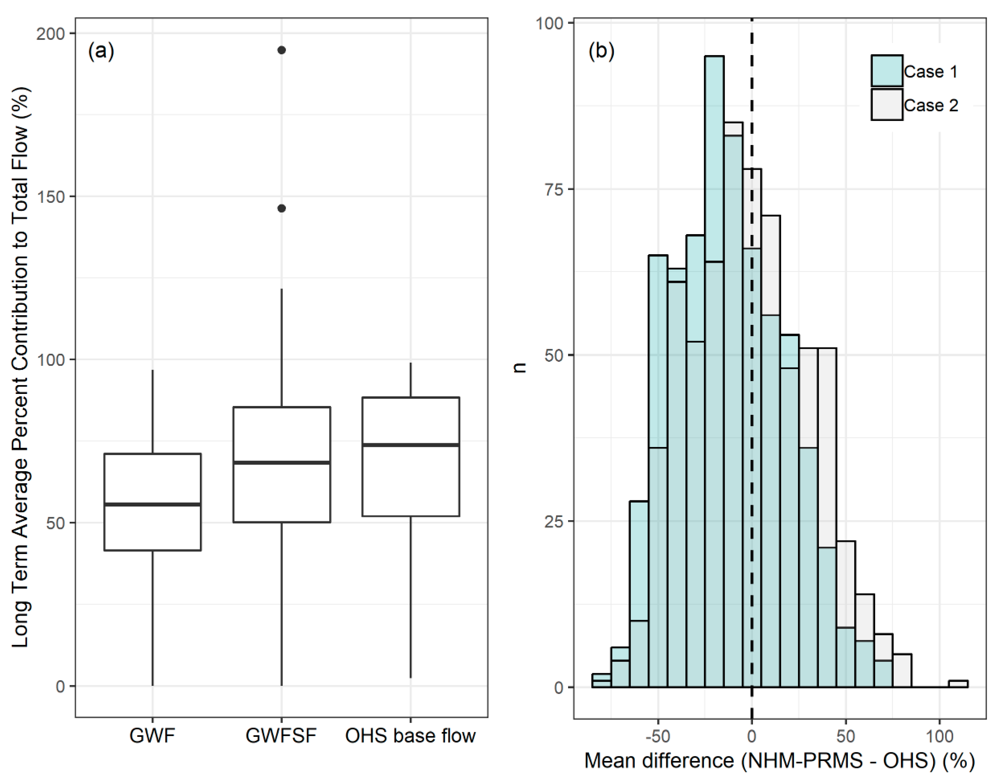
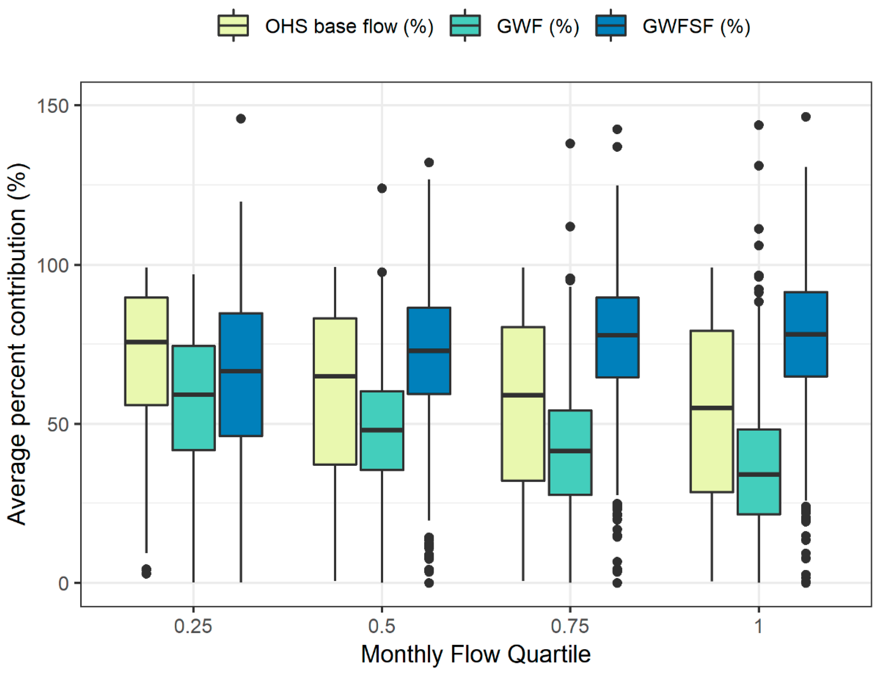
3.2. OHS and NHM-PRMS Outputs: Comparison

Of the original 825 study sites, 662 study sites have acceptable OHS models and base flow estimates, NHM-PRMS watershed drainage area within 10% of reported drainage area in NWIS, and observed discharge and specific conductance data between WY1983 and WY2016 to be compared with simulated flow from NHM-PRMS. Most study sites derived base flow using the SCfit OHS model (554), while less than one sixth of the sites use the sin-cos OHS model (98). The comparison watersheds range from 3.13 km² to 14,300 km² and are evenly distributed across the country (Figure S7).

The averaging timestep (annual and monthly) used in the overall comparisons showed little to no difference among the distribution shape of long-term average volumetric or percent contributions to total flow and had little influence on the overall average percent contribution difference between GWF, GWFSF, and OHS base flow to total flow (Figures S8–S10).

This was expected as the timesteps were all generated from the daily output and any difference observed would be due to averaging.

Long-term average percent contribution comparisons between OHS-estimated base flow to total streamflow and NHM-PRMS subsurface outputs (GWF, GWFSF) to seg_outflow revealed that the NHM-PRMS partitioning of subsurface flow is slightly less than the partitioning of OHS-estimated base flow to total flow (Figure 8a). This is supported by the long-term average percent contribution to total flow, as well as the mean differences between the percent contribution of OHS base flow to streamflow versus percent contribution of GWF to seg_outflow (case 1) and the percent contribution of OHS base flow to streamflow versus percent contribution of GWFSF to seg_outflow (case 2; Figure 8b). Of the two NHM-PRMS output variables, the percent contribution of GWFSF to seg_outflow is generally more similar to OHS base flow estimates than the percent contribution of only GWF to seg_outflow because the distribution of the mean difference for case 2 is centered near zero (Figure 8b).

Examining NHM-PRMS components over normalized monthly flow quartiles suggests that both GWF and GWFSF for the 0.25 and 0.5 normalized flow quartiles are most similar to the lower and higher ranges of average monthly OHS base flow percent contribution (Figure 9).

However, for the normalized flow quartiles of 0.75 and 1, both NHM-PRMS components become more dissimilar to OHS base flow, with GWFSF contributions becoming greater and GWF contribution slightly decreasing more so than OHS base flow contributions.

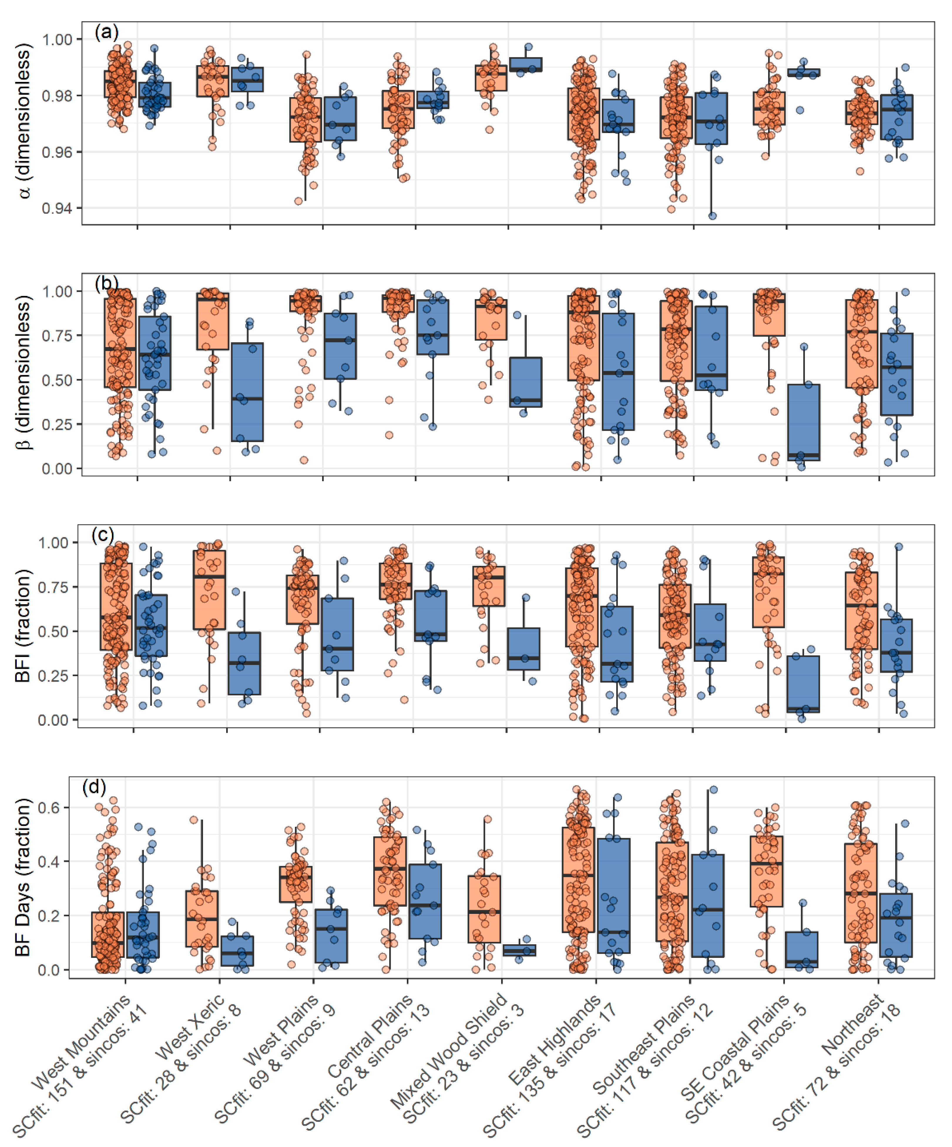
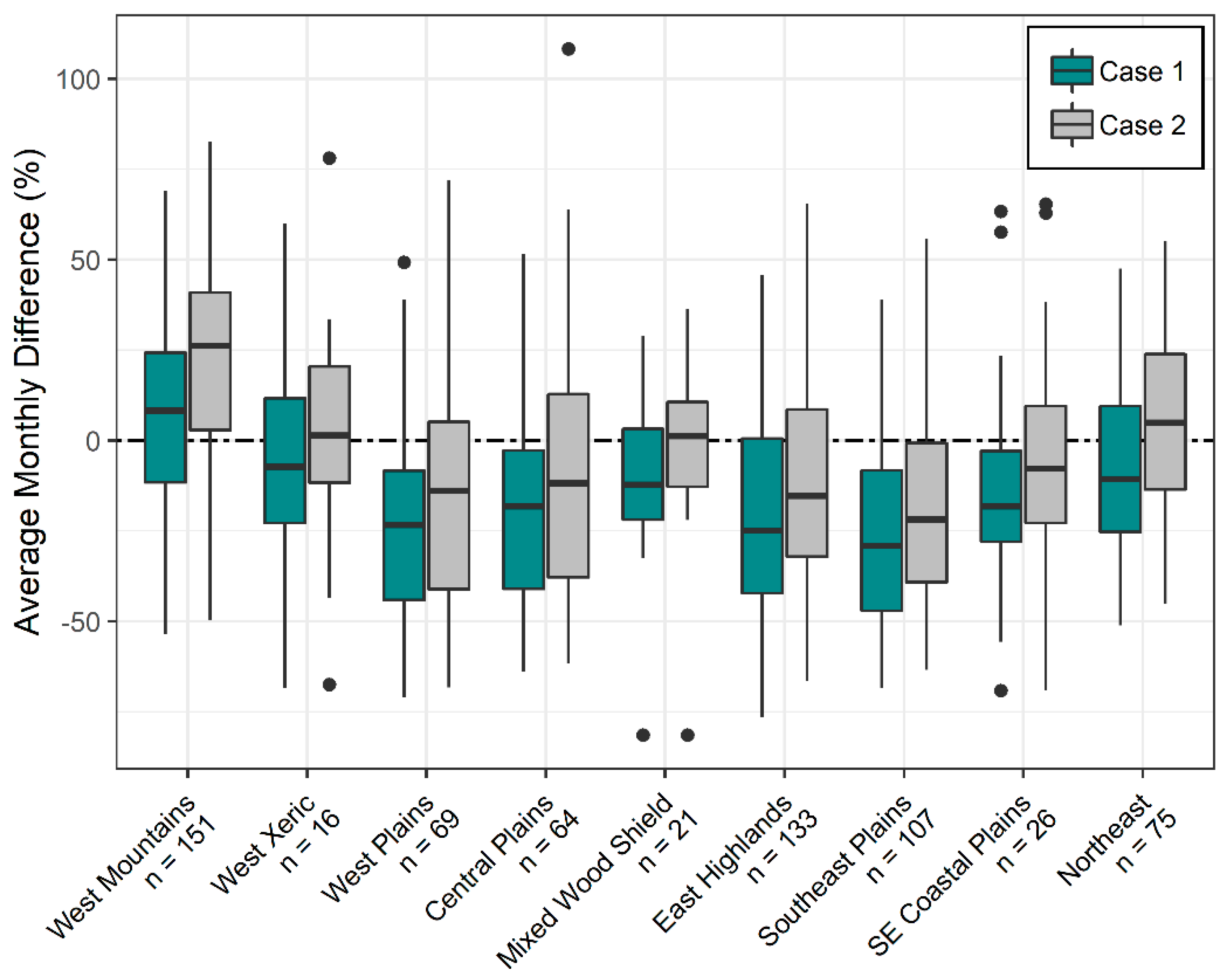
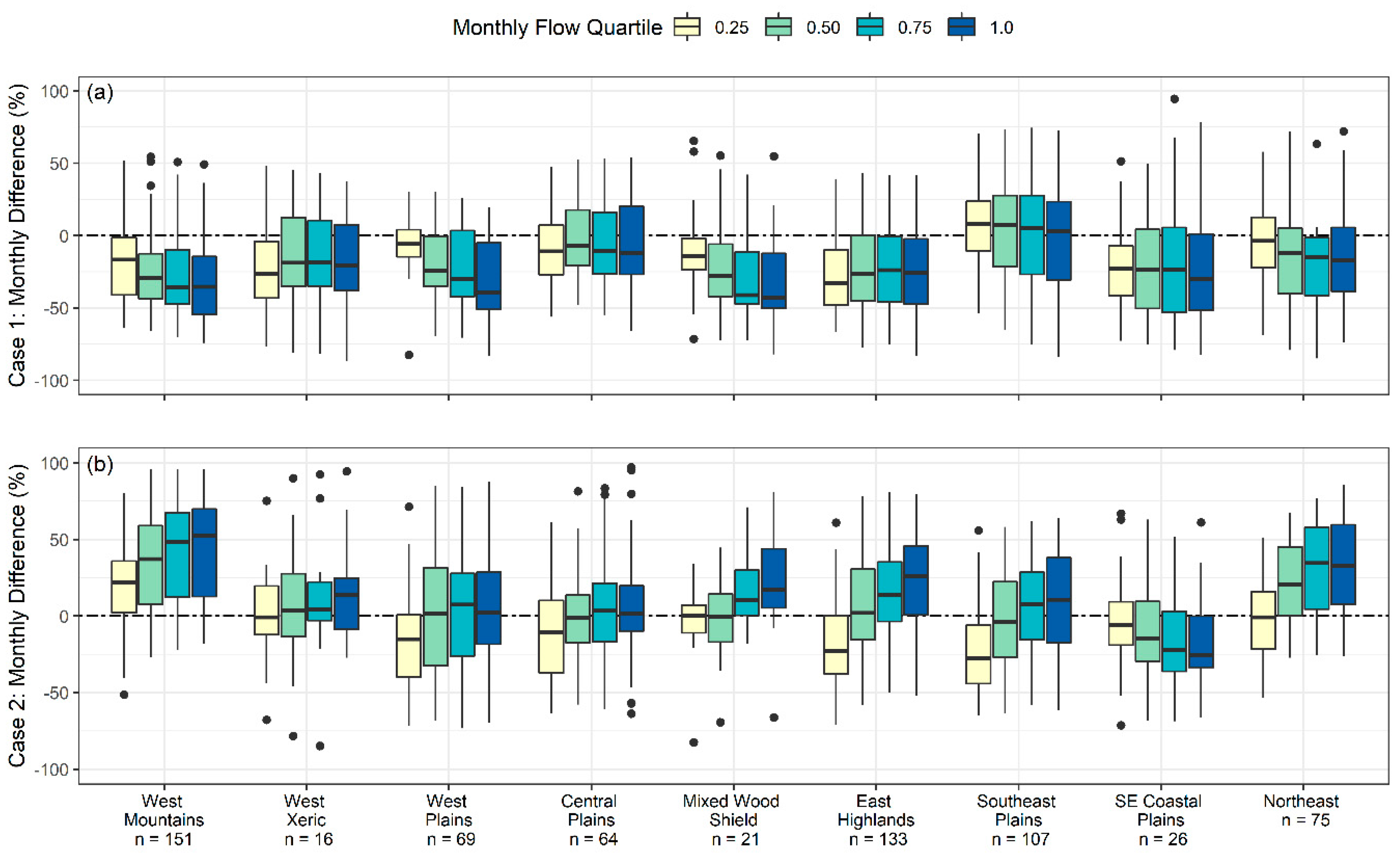
3.2.1. Comparisons by Aggregated Ecoregion

The percent contribution difference across ecoregions and by normalized monthly flow quartiles shows how regionally comparable NHM-PRMS simulated base flow and OHS base flow are across the CONUS and during what type of monthly flow quartile. For most monthly flow quartiles and ecoregions, considering the GWF contribution to total flow as base flow underestimates the OHS base flow contribution to total flow (Figure 10).

One exception to this is the West Mountains ecoregion, in which all flow quartiles match well to OHS base flow with a median difference across flow quartiles ranging from 3–9% (Figure 11a).

Among the low-flow months in the Mixed Wood Shield and West Xeric ecoregions, the percent contributions difference between the GWF and OHS base flow also have good agreement. Additionally, the percent contribution differences in the West Xeric, Northeast, East Highlands, and Southeast Plains have similar medians across flow quartiles, while the Mixed Wood Shield, Central Plains, and Southeast Coastal Plains ecoregions have more variation in the distributions with flow, with lower flows being a better match to OHS base flow contributions and higher flows further from the OHS base flow determination.

When the combination of GWFSF is considered as NHM-PRMS base flow, NHM-PRMS base flow percent contributions are greater than OHS base flow contributions in the western US (West Mountains, West Xeric ecoregions) and in the Northeast, and consistently lower in the middle of the CONUS (Figure 10). There is also more variation in distributions among flow quartile when GWFSF is considered to represent NHM-PRMS base flow, with medians that progressively increase from low to high monthly flow quartiles (Figure 11b). This pattern is exhibited in the East Highlands, Mixed Wood Shield, Southeast Plains, and West Mountains. A similar pattern is exhibited in the Central Plains, Northeast, and West Plains with the exception that the median difference for months in the 0.50–0.75 and 0.75–1.00 quartiles are almost equivalent or slightly decrease. An opposite pattern appears in the Southeast Coastal Plains, with an incremental decrease in the medians from low to high monthly flow quartiles. In general, the GWFSF components in the West Xeric appear to be most similar to OHS base flow with smaller ranges for all monthly flow quartiles and median differences around 0% or slightly higher.

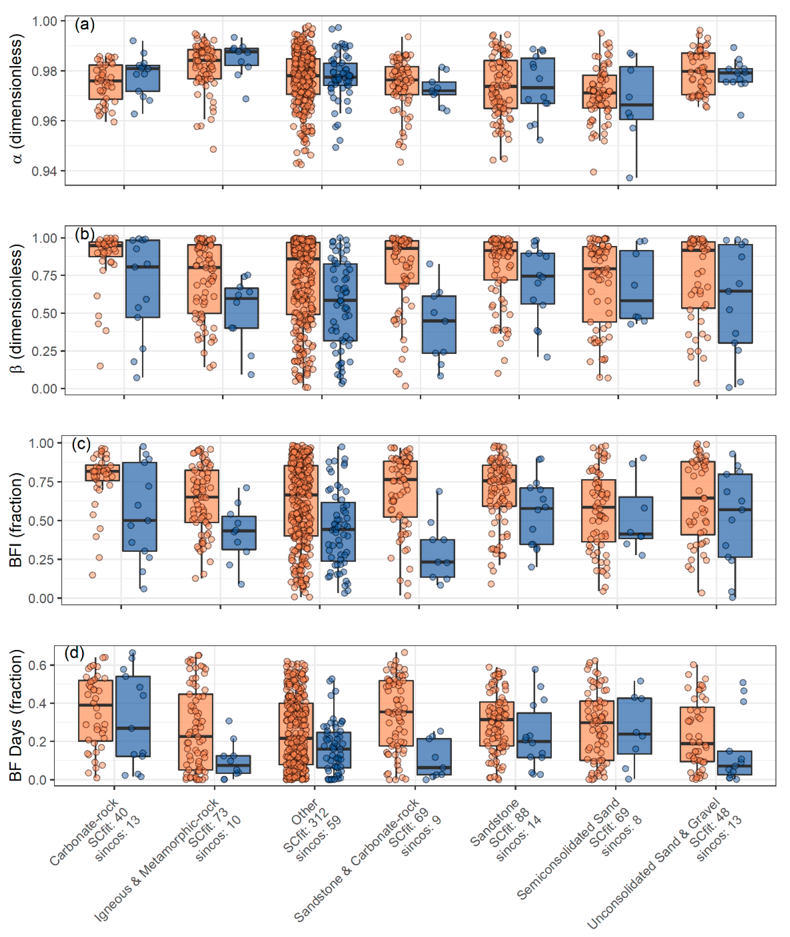
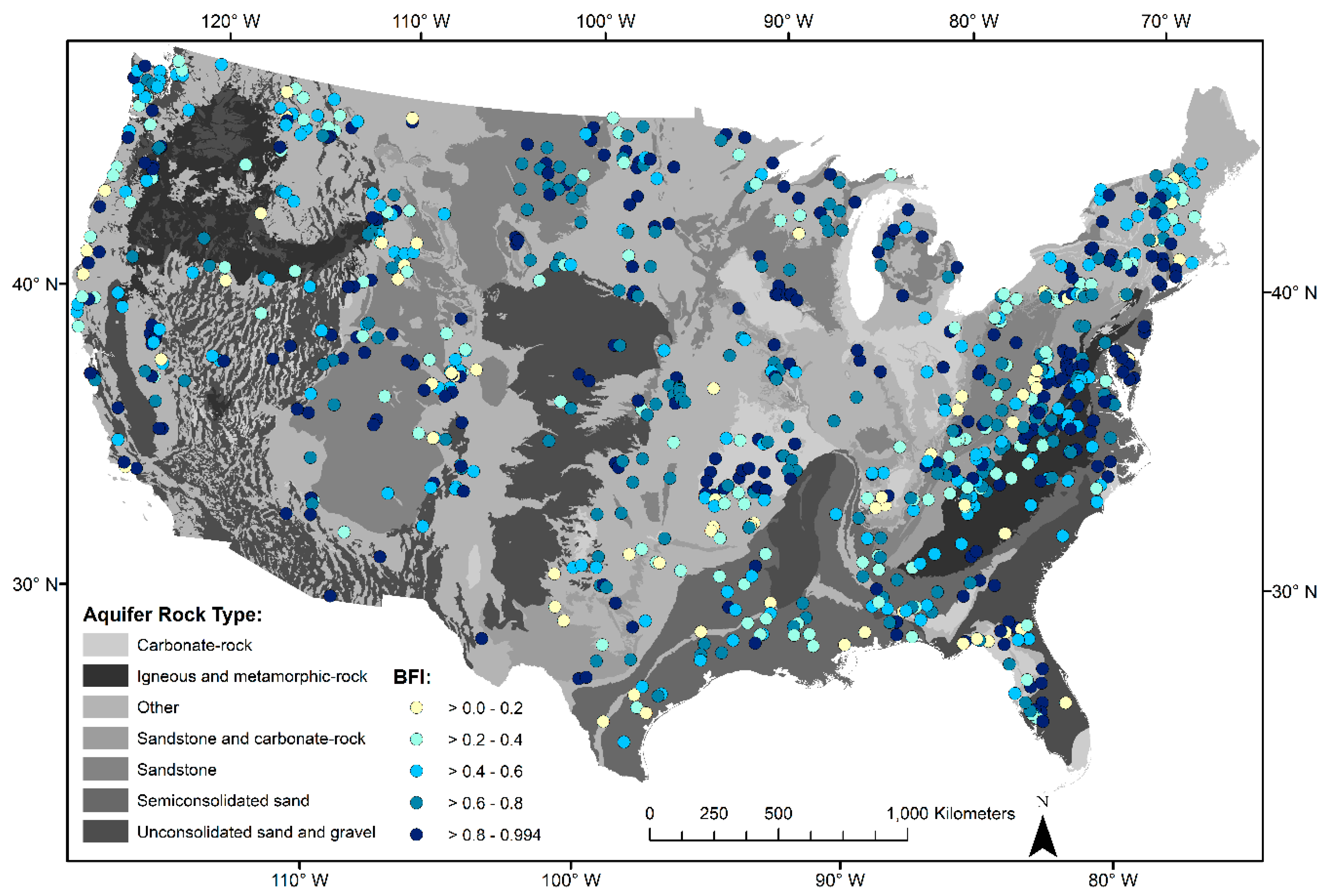
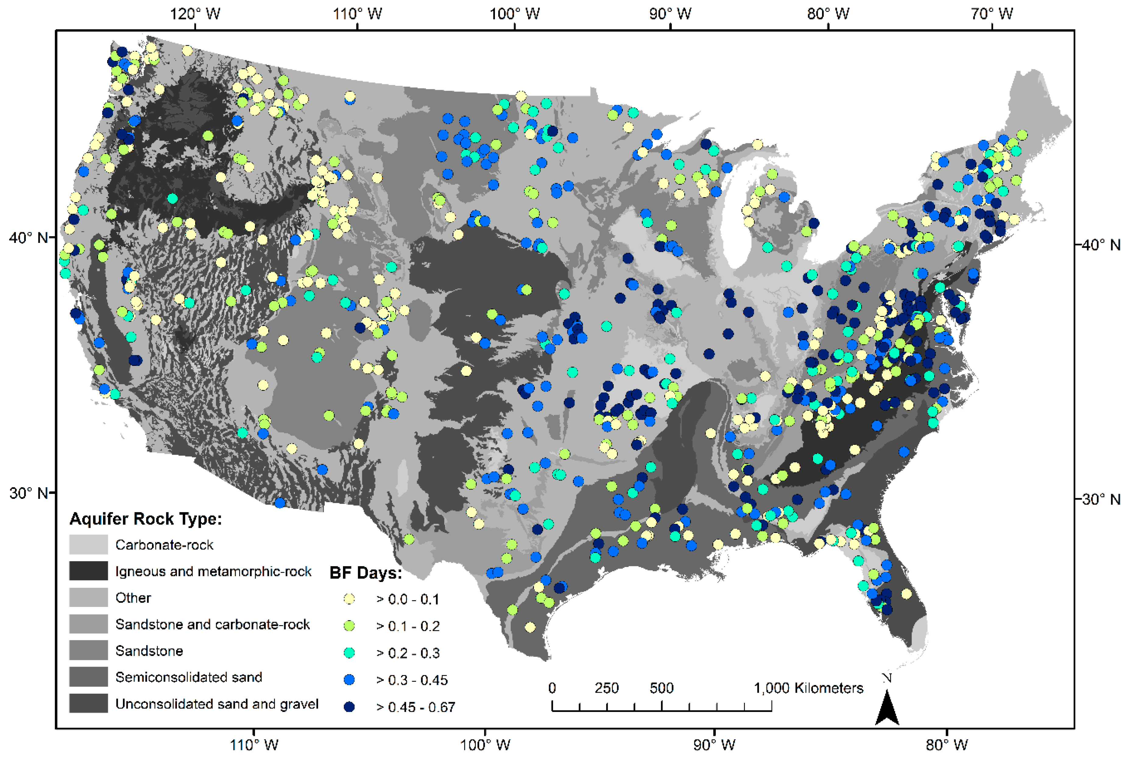
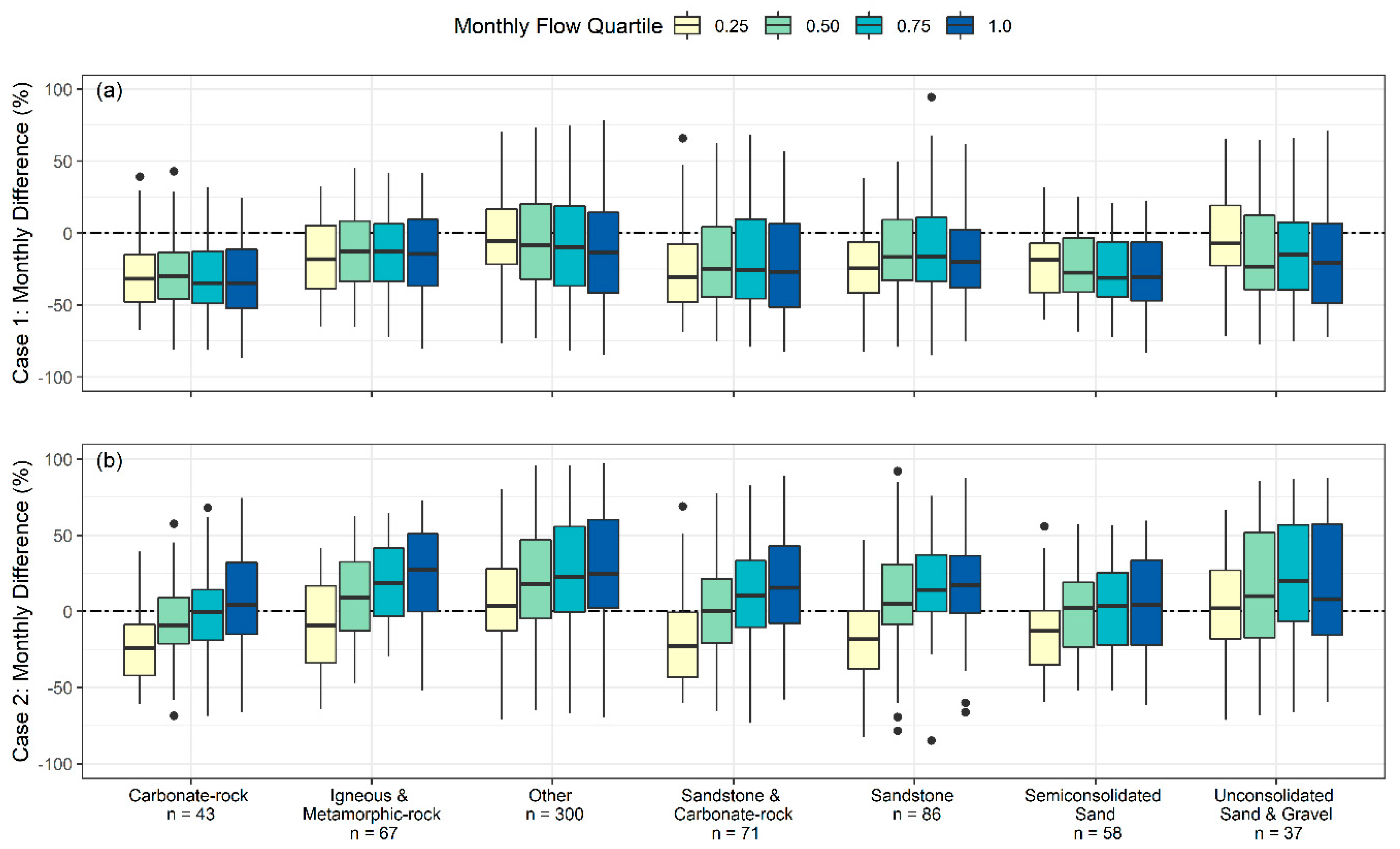
3.2.2. Comparisons by Aquifer Rock Type

The NHM-PRMS base flow contribution of GWF is only slightly lower than the OHS-defined base flow estimates for all defined aquifer rock types and for most flow quartiles (Figure 12 and Figure 13).

The aquifer rock type category of ‘other’ is the closest match to OHS-defined base flow (Figure 12). The normalized monthly flow quartiles of the mean difference of base flow percent contribution to total streamflow between NHM-PRMS base flow and OHS base flow also revealed little difference across varying aquifer rock types within the CONUS (Figure 13). Sandstone aquifers and unconsolidated sand and gravel aquifers had more noticeable differences in the interquartile ranges of normalized monthly flow quartiles, whereas carbonate rock, igneous and metamorphic rock, and semi-consolidated sand aquifers had similar interquartile ranges of normalized monthly flow quartiles, especially during the lowest flow quartiles. Medians of the mean monthly difference among monthly flow quartiles do not substantially differ among any of the aquifer rock types, except for in unconsolidated sand and gravel category where low flows are a closer match to OHS base flow.

A similar pattern is identified among ecoregions emerges among aquifer rock types when GWFSF is considered NHM-PRMS base flow, in that there are progressive increases among the medians of mean monthly difference from low to high monthly flow quartiles (Figure 13b). The NHM-PRMS base flow in the low-flow monthly quartiles among sandstone, semi-consolidated sand, carbonate rock, and sandstone and carbonate rock aquifers have interquartile ranges that are less than the OHS base flow contribution. While the NHM-PRMS base flow percent contribution among aquifer types consisting of “other” and unconsolidated sand and gravel are generally greater than the OHS base flow percent contribution, similar to igneous and metamorphic rock aquifers for 0.5–1.0 quartile flow quartiles. Overall, the mean monthly differences between GWFSF and OHS base flow are the most minimal in the semi-consolidated sand aquifer rock type apart from the low-flow quartile.

4. Discussion

4.1. OHS Performance across the CONUS

The results of this study demonstrate the applicability of the OHS method, and both model types of SCfit and sin-cos across the CONUS, with no apparent pattern in β, BFI, and BF Days with respect to geographic location (Figure 1), watershed drainage area (Figure 2), stream density (Figure S1), mean watershed slope (Figure S3), percent of precipitation composed of snow (Figure S3), estimated annual runoff (Figure S4), mean-annual precipitation and evapotranspiration (Figure S4), or percent land cover composed of irrigated agriculture or perennial ice/snow (Figure S5). This suggests that OHS is applicable across diverse watersheds and hydroclimates but renders the idea of regionalization of β, BFI, and BF Days challenging. Values of α showed patterns with watershed slope, percent of precipitation composed of snow, and the mean-annual precipitation (Figure S2), however, this is related to how α was derived from the NHM-PRMS. Ultimately, the randomness between watershed characteristics and OHS output supports the idea that multiple regression or dimension reduction methods may be better suited for regionalization of base flow estimates.

In the CONUS, a greater number of SCfit model types were accepted than sin-cos model types (with no spatial pattern to this finding), suggesting that some streams may have a stronger seasonal specific conductance signal than others and/or that there are more streams with flashier stream specific conductance that the SCfit model type is better equipped to represent because of the method’s treatment of outliers. In the SCfit model type, peaks and outliers in stream specific conductance are found using a peak-fitting algorithm and are fit instead of “smoothed” as in the sin-cos model type. The differences in how each model handles the fitting of stream specific conductance could be the reason why we see slightly higher estimates of BFI and BF Days among SCfit model types versus sin-cos model types, as the greater number of peaks identified in the stream specific conductance from the SCfit model type would suggest greater base flow. Overall, these differences in the output values were minor and therefore ignored, since the best model type for each site was chosen by the greatest NSE value.

Grouped by ecoregion (Figure 4) or aquifer rock type (Figure 5), values of α and β display wide ranges that generally overlap indicating greater variance within an ecoregion or aquifer type than between them. Again, the SCfit model type produces overall greater values and occasionally more consistent and narrower distributions of β, BFI, and BF Days among various ecoregions and aquifer types than the sin-cos model type, suggesting that differences between the OHS models should be evaluated further instead of focusing on spatial characteristic differences.

A map of the long-term average BFI (Figure 6) also demonstrates the variability across the landscape and with underlying rock type. Potential differences can be seen on the leeward and windward sides of mountain ranges, but this needs further investigation. BF Days does not necessarily follow the same pattern as the long-term BFI (Figure 7). There is a tendency for the fraction of base flow days to be relatively low in the western US (especially in the ecoregions, West Mountains and West Xeric), independent of the long-term average BFI (Figure 4 and Figure 6). This may be related to the frequency of precipitation events or period of data examined within El Nino-Southern Oscillation phases [59], and/or due to large contributions to streamflow from snowmelt. However, comparison of BFI versus BF Days as functions of snow percent of precipitation and watershed mean elevation (Figure 3) indicates that the BF Days for a given BFI are generally smaller as elevation and the snow percent contribution to total precipitation increase. This implies that mountainous areas are characterized by fewer BF Days and the prevalence of mountainous, snow-dominated watersheds are greater in the western US as opposed to the central and eastern US. Thus, snow influences are likely a reason why we see fewer days at 100% base flow in the western US.

4.2. OHS Comparison to the NHM-PRMS

Initial comparisons of the NHM-PRMS to OHS base flow suggested that GWFSF components are most analogous to OHS base flow, however, analysis by ecoregion, aquifer type, and flow quartiles reveals the complicated nature of how flow is allocated within the NHM-PRMS, how OHS base flow varies with flow, and that one simple combination of NHM-PRMS subsurface components is not akin to OHS base flow in all regions across the CONUS.

Of the study analyses, GWF is most analogous to OHS base flow in the aggregated ecoregions of the West Mountains and the Northeast for all flow quartiles, in the lowest flow quartiles of the Mixed Wood Shield and West Xeric ecoregions, and in aquifer rock types categorized as “other”. In addition, the aquifer rock type of “other” is assigned to the majority of sites within the West Mountains (70% of sites), Northeast (79%), West Xeric (44%), and Mixed Wood Shield (76%) ecoregions (Table S1); thus this spatial overlap may be compounding the analogous behavior between OHS base flow and GWF amongst these ecoregions and aquifer types, and/or it is likely a coincidence since many of the study sites were categorized as the aquifer rock type “other”. This coincidence is supported by comparisons between OHS base flow and GWFSF. Of the study analyses, GWFSF is most analogous to OHS base flow in the aggregated ecoregion of the West Xeric for all flow quartiles, in the Central Plains for most flow quartiles, and in aquifer rock types categorized as “semi-consolidated sand”. However, the West Xeric has only 3% of its study sites categorized as being in a semi-consolidated sand aquifer and the Central Plains has 0% study sites (Table S1). Therefore, the spatial overlap of aquifer type and ecoregion, and the comparison between OHS base flow and NHM-PRMS components are not directly connected.

Comparisons among flow quartiles reveal how OHS base flow, GWF, and SF water vary in certain regions and in the timing of their contributions to total flow. With greater total flows, the OHS base flow distribution across the comparison sites becomes wider in range, with an overall smaller percent contribution to total flow (Figure 9). This makes sense, as larger amounts of precipitation associated with higher flows should lower the base flow fractional contribution to total flow. This pattern exists with the GWF component as well, among ecoregions and aquifer types (Figures S11 and S12), implying OHS base flow and GWF have a similar definition of flow. However, the opposite scenario is true with the SF component, as SF contributes more to total flow during greater flows, suggesting this component is more representative of precipitation than subsurface inputs (Figure 9, Figures S11 and S12). Therefore, SF cannot be added to GWF during all periods of the hydrograph, otherwise the NHM-PRMS representation of base flow will be larger than OHS-estimated base flow during higher flows (ex: in most aquifer rock types, in the West Mountains, Northeast, Southeast Plains, East Highlands, and in the Mixed Wood Shield ecoregions). In the West Xeric and Central Plains ecoregions, SF still increases in contribution to total flow during higher flows (Figure S11), but the GWF contribution in these regions counterbalance or even suppress the precipitation input so that the differences between OHS and GWFSF in these ecoregions are consistent across various flows (Figure 11).

4.3. Use of OHS as a Calibration Tool

To use OHS as a calibration and/or validation method for the NHM-PRMS or any hydrologic model, model components that are analogous to base flow need to be identified. In the NHM-PRMS case, two subsurface components, SF and GWF could both theoretically represent base flow. However, GWF generally contributes a smaller portion of total flow than the OHS base flow and GWFSF occasionally contributes too much to the total flow compared to OHS-estimated base flow, especially during greater streamflow and precipitation. Therefore, there are several possible solutions to calibrate and validate these components to OHS base flow.

Since the addition of the SF NHM-PRMS component can contribute more flow to total flow than OHS allocates to total flow, the SF component could potentially be split into two components, with one component consisting of the SF base flow fraction and the remaining component consisting of a SF quick flow fraction. Similarly, Miller and others (2017) [60] proposed splitting the hydrograph into three sources rather than two to better represent varying chemical pathways to streams; with a stream composed of a quick flow component, “quick” base flow component, and a “slow” base flow component. In the NHM-PRMS, the SF base flow component could be the sum of the GWF component and the amount of flow needed to reproduce OHS base flow and may be representative of Miller and others (2017) [60] definition of a “concentrated quick flow” component. In addition, results from OHS can be used to calibrate parameters that control the flow between gravity and groundwater reservoirs (ssr2gw_rate) that may allow for GWFSF to align more with OHS-derived base flow. Another option would be to perform OHS on NHM-PRMS statically generated streamflow (seg_outflow) with observed specific conductance data to explore aspects of incorporating water quality into the model to constrain or calibrate/validate estimates of GWF and SF to the outflow segment.

As mentioned earlier, the memory of upstream HRUs and segments are not taken into consideration in the NHM-PRMS byHRU calibration, however, future implementation of flow routing components may greatly improve comparisons between OHS-derived base flow and base flow components from NHM-PRMS such that new variables may not be needed. Inclusion of upstream memory in flow routing components into the NHH-PRMS would allow daily values of NHM-PRMS components at a model outlet to be directly compared to daily OHS results, thus better capturing storm events and providing an opportunity for more detailed calibration.

4.4. Limitations of OHS & NHM-PRMS

Limitations of the OHS approach were described in Raffensperger et al. (2017) [30]. In summary, limitations result from the assumptions implicit in the conceptual model, the RDF method, and the approach taken to impose chemical mass balance (including tracer choice). The impact of the OHS limitations may be evidenced by poor OHS model results; conversely, poor model fit may provide an indication that two-component separation does not adequately describe the hydrologic system’s runoff response. Two-component separation may be insufficient to characterize systems with more complex or diverse hydrologic compartments or components (such as interflow or subsurface storm-flow, movement of soil moisture, macropore flow) or with human modification (including diversions, dams, point sources and sinks, artificial drainage, and others). In addition, non-conservative tracer mixing could reduce the difference or confuse the signals between base flow and quick flow streamflow components in OHS, and especially interfere with how the SCfit model pinpoints peaks in specific conductance as entirely base flow.

As previously mentioned, the NHM-PRMS static parameters, gwflow_coef and soil permeability, do not address antecedent conditions, human disturbance, and temporal change, and is likely one reason we see differences in the GWFSF contribution to total flow over various flow quartiles. Therefore, the results from OHS may provide an opportunity to expand dynamic parameter capabilities within NHM-PRMS. Restrictions of resolution (spatial and temporal) are always to be considered and improved upon with every iteration of the NHM-PRMS or any hydrologic model, and the absence of flow routing in the current version of the NHM-PRMS is also a limiting factor in our comparison between OHS and the NHM-PRMS.

4.5. Future Directions

The application of OHS to hundreds of gages throughout the CONUS is an example of how this method could be implemented in real-time at all gages with continuous discharge data and some recurring measurements of specific conductance. This would provide real-time datasets to be used in the NHM-PRMS or other national-extent hydrologic models for calibration and validation, and general hydrologic process improvement. In addition to data delivery, uncertainty estimates need to be quantified to provide a better calibration dataset for hydrologic models. Trends in base flow contribution would give insight into the response of surface-water and groundwater exchange to climatic and anthropogenic drivers. Instead of examining spatial and temporal differences between OHS base flow, GWF, GWFSF, and SF by ecoregion, aquifer type, and normalized monthly flow quartiles, analysis of these components and their contribution changes over the period of record for each site in relation to climate or drought influences could highlight geographic, watershed-related, and hydrologic discrepancies that need further investigation. Defining base flow more thoroughly in hydrologic models would also aid in water-quality prediction assessments.

5. Conclusions

OHS is an objective, reproducible, automated method that is applicable in a variety of watersheds throughout the CONUS (77% of the basins tested in this study) of varying drainage area, stream density, slope, elevation, precipitation, evapotranspiration, runoff, and land cover. Data requirements for this method are simple compared to end-member mixing analysis, yet OHS still incorporates watershed hydrogeochemical data so that observed and simulated chemistry can be used to judge how well OHS performed, unlike many graphical hydrograph separation techniques. Therefore, OHS is a suitable calibration and/or validation tool for hydrologic models analyzing base flow contributions to streams and rivers.

OHS estimates of long-term average BFI suggest that base flow comprises a large portion of streamflow on average across the CONUS without distinct geographic patterns, whereas estimates of BF Days is lower in the western US compared to the rest of the CONUS. Comparing base flow analogous components of the NHM-PRMS to OHS estimates reveal that the GWF percent contributions are frequently lower than base flow estimates provided by OHS, but both estimates decrease in contribution with increasing total flow, suggesting these two components are most similar in terms of the type of flow they represent. GWFSF percent contributions are occasionally greater than base flow estimated by OHS, especially during higher total flows and the SF component generally increases in contribution during higher total flows indicating its close connection to precipitation and representation of a quick flow signal. Comparisons of OHS, GWF, and GWFSF across aquifer type and ecoregion suggest little to no patterns spatially, with certain ecoregions or aquifer types having only slightly better results than others.

Defining base flow is important for the prediction of water quantity and quality, especially in terms of answering whether changes in water quality are driven by changes in source water chemistry or changes in the quantity of source water contributing to the stream. However, this issue is circular and needs hydrologic models to answer these sorts of questions. OHS is a valuable affirmation method for hydrologic models as it produces valuable outputs that can be used to evaluate and validate hydrologic model outputs.

References

1. Price, K. Effects of watershed topography, soils, land use, and climate on baseflow hydrology in humid regions: A review. Prog. Phys. Geogr. Earth Environ. 2011, 35, 465–492. [Google Scholar] [CrossRef]
2. Hall, F.R. Base flow recessions—A review. Water Resour. Res. 1968, 4, 973–983. [Google Scholar] [CrossRef]
3. Miller, M.P.; Buto, S.G.; Susong, D.D.; Rumsey, C.A. The importance of base flow in sustaining surface water flow in the Upper Colorado River Basin. Water Resour. Res. 2016, 52, 3547–3562. [Google Scholar] [CrossRef]
4. Song, X.; Chen, X.; Stegen, J.; Hammond, G.; Song, H.S.; Dai, H.; Graham, E.; Zachara, J.M. Drought Conditions Maximize the Impact of High-Frequency Flow Variations on Thermal Regimes and Biogeochemical Function in the Hyporheic Zone. Water Resour. Res. 2018, 54, 7361–7382. [Google Scholar] [CrossRef]
5. Smakhtin, V.U. Low flow hydrology: A review. J. Hydrol. 2001, 240, 147–186. [Google Scholar] [CrossRef]
6. Van Loon, A.F. Hydrological drought explained. Wiley Interdiscip. Rev. Water 2015, 2, 359–392. [Google Scholar] [CrossRef]
7. Larsen, L.G.; Woelfle-Erskine, C. Groundwater Is Key to Salmonid Persistence and Recruitment in Intermittent Mediterranean-Climate Streams. Water Resour. Res. 2018, 54, 8909–8930. [Google Scholar] [CrossRef]
8. Nuhfer, A.J.; Zorn, T.G.; Wills, T.C. Effects of reduced summer flows on the brook trout population and temperatures of a groundwater-influenced stream. Ecol. Freshw. Fish. 2017, 26, 108–119. [Google Scholar] [CrossRef]
9. Somers, K.A.; Bernhardt, E.S.; McGlynn, B.L.; Urban, D.L. Downstream Dissipation of Storm Flow Heat Pulses: A Case Study and its Landscape-Level Implications. J. Am. Water Resour. Assoc. 2016, 52, 281–297. [Google Scholar] [CrossRef]
10. Santhi, C.; Allen, P.M.; Muttiah, R.S.; Arnold, J.G.; Tuppad, P. Regional estimation of base flow for the conterminous United States by hydrologic landscape regions. J. Hydrol. 2008, 351, 139–153. [Google Scholar] [CrossRef]
11. Essaid, H.I.; Caldwell, R.R. Evaluating the impact of irrigation on surface water-gorundwater interaction and stream temperature in an agricultural watershed. Sci. Total Environ. 2017, 599, 581–596. [Google Scholar] [CrossRef]
12. Trauth, N.; Musolff, A.; Knöller, K.; Kaden, U.S.; Keller, T.; Werban, U.; Fleckenstein, J.H. River water infiltration enhances denitrification efficiency in riparian groundwater. Water Res. 2018, 130, 185–199. [Google Scholar] [CrossRef]
13. Regan, R.S.; Markstrom, S.L.; Hay, L.E.; Viger, R.J.; Norton, P.A.; Driscoll, J.M.; LaFontaine, J.H. Description of the National Hydrologic Model for Use with the Precipitation-Runoff Modeling System (PRMS); U.S. Geological Survey Techniques and Methods 6-B9; USGS: Reston, VA, USA, 2018; p. 38. [CrossRef]
14. Regan, R.S.; Juracek, K.E.; Hay, L.E.; Markstrom, S.L.; Viger, R.J.; Driscoll, J.M.; LaFontaine, J.H.; Norton, P.A. The US Geological Survey National Hydrologic Model infrastructure: Rationale, description, and application of a watershed-scale model for the conterminous United States. Environ. Model. Softw. 2019, 111, 192–203. [Google Scholar] [CrossRef]
15. Boussinesq, J. Essai sur la théorie des eaux courantes. In Mémoires Présentés par Divers Savants a l’Academic des Sciences de l’Institut National de France; Tome XXIII N: Paris, France, 1877; p. 23. [Google Scholar]
16. Freeze, R.A. Role of subsurface flow in generating surface runoff: 1. Base flow contributions to channel flow. Water Resour. Res. 1972, 8, 609–623. [Google Scholar] [CrossRef]
17. White, K.E.; Sloto, R.A. Base Flow Frequency Characteristics of Selected Pennsylvania Streams; U.S. Geological Survey Water-Resources Investigation Report 90-4160; USGS: Reston, VA, USA, 1990; p. 66. [CrossRef]
18. Rutledge, A.T.; Daniel, C.C. III. Testing an automated method to estimate ground-water recharge from streamflow records. Groundwater 1994, 32, 180–189. [Google Scholar] [CrossRef]
19. Nathan, R.J.; McMahon, T.A. Evaluation of automated techniques for base flow and recession analyses. Water Resour. Res. 1990, 26, 1465–1473. [Google Scholar] [CrossRef]
20. Rutledge, A.T. Computer Programs for Describing the Recession of Ground-Water Discharge and for Estimating Mean Ground-Water Recharge and Discharge from Streamflow Records—Update; U.S. Geological Survey Water-Resources Investigations Report 98-4148; USGS: Reston, VA, USA, 1998; p. 43. [CrossRef]
21. Rutledge, A.T. Considerations for Use of the RORA Program to Estimate Ground-Water Recharge from Streamflow Records; U.S. Geological Survey Open-File Report 00-156; USGS: Reston, VA, USA, 2000; p. 52. [CrossRef]
22. Barlow, P.M.; Cunningham, W.L.; Zhai, T.; Gray, M.U.S. Geological Survey Groundwater Toolbox, a Graphical and Mapping Interface for Analysis of Hydrologic Data (Version 1.0)—User Guide for Estimation of Base Flow, Runoff, and Groundwater Recharge from Streamflow Data; U.S. Geological Survey Techniques and Methods 3-B10; USGS: Reston, VA, USA, 2015; p. 27. [CrossRef]
23. Hooper, R.P.; Shoemaker, C.A. A comparison of chemical and isotopic hydrograph separation. Water Resour. Res. 1986, 22, 1444–1454. [Google Scholar] [CrossRef]
24. La Sala, A.M., Jr. New Approaches to Water-Resources Investigations in Upstate New York. Groundwater 1967, 5, 6–11. [Google Scholar] [CrossRef]
25. Miller, M.P.; Susong, D.D.; Shope, C.L.; Heilweil, V.M.; Stolp, B.J. Continuous estimation of base flow in snowmelt-dominated streams and rivers in the Upper Colorado River Basin: A chemical hydrograph separation approach. Water Resour. Res. 2014, 50, 6986–6999. [Google Scholar] [CrossRef]
26. Pinder, G.F.; Jones, J.F. Determination of the ground-water component of peak discharge from the chemistry of total runoff. Water Resour. Res. 1969, 5, 438–445. [Google Scholar] [CrossRef]
27. Stewart, M.; Cimino, J.; Ross, M. Calibration of base flow separation methods with streamflow conductivity. Groundwater 2007, 45, 17–27. [Google Scholar] [CrossRef]
28. Godsey, S.E.; Kirchner, J.W.; Clow, D.W. Concentration-discharge relationships reflect chemostatic characteristics of US catchments. Hydrol. Process. 2009, 23, 1844–1864. [Google Scholar] [CrossRef]
29. Clow, D.W.; Mast, M.A. Mechanisms for chemostatic behavior in catchments: Implications for CO2 consumption by mineral weathering. Chem. Geol. 2010, 269, 40–51. [Google Scholar] [CrossRef]
30. Raffensperger, J.P.; Baker, A.C.; Blomquist, J.D.; Hopple, J.A. Optimal Hydrograph Separation Using a Recursive Digital Filter Constrained by Chemical Mass Balance, with Application to Selected Chesapeake Bay Watersheds; U.S. Geological Survey Scientific Investigations Report 2017-5034; USGS: Reston, VA, USA, 2017; p. 51. [CrossRef]
31. Rimmer, A.; Hartmann, A. Optimal hydrograph separation filter to evaluate transport routines of hydrological models. J. Hydrol. 2014, 514, 249–257. [Google Scholar] [CrossRef]
32. Eckhardt, K. How to construct recursive digital filters for base flow separation. Hydrol. Process. 2005, 19, 507–515. [Google Scholar] [CrossRef]
33. Markstrom, S.L.; Regan, R.S.; Hay, L.E.; Viger, R.J.; Webb, R.M.; Payn, R.A.; LaFontaine, J.H. PRMS-IV, the Precipitation-Runoff Modeling System, Version 4; U.S. Geological Survey Techniques and Methods 6-B7; USGS: Reston, VA, USA, 2015; p. 158. [CrossRef]
34. Falcone, J.A. GAGES-II: Geospatial Attributes of Gages for Evaluating Streamflow; U.S. Geological Survey Dataset Report; USGS: Reston, VA, USA, 2011. [CrossRef]
35. U.S. Geological Survey. USGS Water Data for the Nation: U.S. Geological Survey National Water Information System Database. 2018. Available online: waterdata.usgs.gov/nwis/ (accessed on 1 October 2018). [CrossRef]
36. Sloto, R.A.; Crouse, M.Y. HYSEP: A Computer Program for Streamflow Hydrograph Separation and Analysis; U.S. Geological Survey Water-Resources Investigations Report 96-4040; USGS: Reston, VA, USA, 1996; p. 46. [CrossRef]
37. Rutledge, A.T.; Mesko, T.O. Estimated Hydrologic Characteristics of Shallow Aquifer Systems in the Valley and Ridge, the Blue Ridge, and the Piedmont Physiographic Provinces Based on Analysis of Streamflow Recession and Base Flow; U.S. Geological Survey Report 1422-B; USGS: Reston, VA, USA, 1998; p. 58. [CrossRef]
38. Team, R.C. R: A Language and Environment for Statistical Computing; R Foundation for Statistical Computing: Vienna, Austria, 2018; Available online: www.R-project (accessed on 1 August 2019).
39. Powell, M.J.D. The BOBYQA Algorithm for Bound Constrained Optimization without Derivatives. Department of Applied Mathematics and Theoretical Physics; Technical Report NA2009/06; University of Cambridge: Cambridge, UK, 2009; pp. 26–46. [Google Scholar]
40. Ypma, J. Introduction to nloptr: An R interface to NLopt. Tech. Rep. 2018. Available online: cran.r-project:web/packages/nloptr/vignettes/nloptr.pdf (accessed on 1 August 2019).
41. Borchers, H.W. Pracma: Practical Numerical Math Functions. R package version 2.2.5. 2019. Available online: CRAN.R-project:package=pracma (accessed on 1 August 2019).
42. Nash, J.E.; Sutcliffe, J.V. River flow forecasting through conceptual models part I—A discussion of principles. J. Hydrol. 1970, 10, 282–290. [Google Scholar] [CrossRef]
43. Zecharias, Y.B.; Brutsaert, W. The influence of basin morphology on groundwater outflow. Water Resour. Res. 1988, 24, 1645–1650. [Google Scholar] [CrossRef]
44. Regan, R.S.; LaFontaine, J.H. Documentation of the Dynamic Parameter, Water-Use, Stream and Lake Flow Routing, and Two Summary Output Modules and Updates to Surface-Depression Storage Simulation and Initial Conditions Specification Options with the Precipitation-Runoff Modeling System (PRMS); U.S. Geological Survey Techniques and Methods 6-B8; USGS: Reston, VA, USA, 2017; p. 60. [CrossRef]
45. Markstrom, S.L.; Hay, L.E.; Clark, M.P. Towards simplification of hydrologic modeling: Identification of dominant processes. Hydrol. Earth Syst. Sci. 2016, 20, 4655–4671. [Google Scholar] [CrossRef]
46. Viger, R.J.; Bock, A. GIS Features of the Geospatial Fabric for National Hydrologic Modeling; USGS: Reston, VA, USA, 2014. [CrossRef]
47. U.S. Geological Survey; U.S. Environmental Protection Agency. National Hydrography Dataset Plus—NHDPlus Version 1.0 Dataset. Available online: http://horizon-systems.com/NHDPlus/NHDPlusV1_home.php (accessed on 1 October 2018).
48. Driscoll, J.M.; Markstrom, S.L.; Regan, R.S.; Hay, L.E.; Viger, R.J. National Hydrologic Model Parameter Database: 2017-05-08; USGS: Reston, VA, USA, 2017. [CrossRef]
49. Viger, R.J. Preliminary Spatial Parameters for PRMS Based on the Geospatial Fabric, NCLD2001 and SSURGO; USGS: Reston, VA, USA, 2014. [CrossRef]
50. LaFontaine, J.H.; Hay, L.E.; Viger, R.J.; Regan, R.S.; Markstrom, S.L. Effects of climate and land cover on hydrology in the Southeastern US: Potential impacts on watershed planning. J. Am. Water Resour. Assoc. 2015, 51, 1235–1261. [Google Scholar] [CrossRef]
51. LaFontaine, J.H.; Hart, R.M.; Hay, L.E.; Farmer, W.H.; Bock, A.R.; Viger, R.J.; Markstrom, S.L.; Regan, R.S.; Driscoll, J.M. Simulation of Water Availability in the Southeastern United States for Historical and Potential Future Climate and Land-Cover Conditions; U.S. Geological Survey Scientific Investigations Report 2019–5039; USGS: Reston, VA, USA, 2019; p. 83. [CrossRef]
52. Hay, L.E. Application of the National Hydrologic Model Infrastructure with the Precipitation-Runoff Modeling System (NHM-PRMS), byHRU Calibrated Version; USGS: Reston, VA, USA, 2019. [CrossRef]
53. Duan, Q.Y.; Sorooshian, S.; Gupta, V.K. Effective and efficient global optimization for conceptual rainfall-runoff models. Water Resour. Res. 1992, 28, 1015–1031. [Google Scholar] [CrossRef]
54. Duan, Q.Y.; Gupta, V.K.; Sorooshian, S. Shuffled complex evolution approach for effective and efficient global minimization. J. Optim. Theory Appl. 1993, 76, 501–521. [Google Scholar] [CrossRef]
55. Duan, Q.Y.; Sorooshian, S.; Gupta, V.K. Optimal use of the SCE-UA global optimization method for calibration watershed models. J. Hydrol. 1994, 158, 265–284. [Google Scholar] [CrossRef]
56. Thornton, P.E.; Thornton, M.M.; Mayer, B.W.; Wei, Y.; Devarakonda, R.; Vose, R.S.; Cook, R.B. Daymet: Daily Surface Weather Data on a 1-km Grid for North America; Version 3; ORNL DAAC: Oak Ridge, TN, USA, 2016. [CrossRef]
57. U.S. Geological Survey. Principal Aquifers of the 48 Conterminous United States, Hawaii, Puerto Rico, and the U.S. Virgin Islands Version 1.0; U.S. Geological Survey: Reston, VA, USA, 2003. Available online: water.usgs.gov/ogw/aquifer/principal/aquifrp025.xml (accessed on 1 October 2018).
58. Falcone, J.A.; Carlisle, D.M.; Wolock, D.M.; Meador, M.R. GAGES: A stream gage database for evaluating natural and altered flow conditions in the conterminous United States. Ecology 2010, 91, 621. [Google Scholar] [CrossRef]
59. Kunkel, K.E.; Easterling, D.R.; Redmond, K.; Hubbard, K. Temporal variations of extreme precipitation events in the United States: 1895–2000. Geophys. Res. Lett. 2003, 30, 1900. [Google Scholar] [CrossRef]
60. Miller, M.P.; Tesoriero, A.J.; Hood, K.; Terziotti, S.; Wolock, D.M. Estimating Discharge and Nonpoint Source Nitrate Loading to Streams from Three End-Member Pathways Using High-Frequency Water Quality Data. Water Resour. Res. 2017, 53, 10201–10216. [Google Scholar] [CrossRef]
61. Foks, S.S.; Raffensperger, J.P.; Penn, C.A.; Driscoll, J.M. Base Flow Estimation via Optimal Hydrograph Separation at CONUS Watersheds and Comparison to the National Hydrologic Model—Precipitation-Runoff Modeling System by HRU Calibrated Version; USGS: Reston, VA, USA, 2019. [CrossRef]
Figure 1. Select GAGES-II locations that have accepted OHS models (SCfit and sin-cos) or rejected OHS models (pink triangles). Accepted models span the CONUS and a variety of aquifer rock types.
Water 11 01629 g001
Figure 2. OHS model input parameters ((a) α and (b) β) and output variables ((c) BFI and (d) BF Days) displayed by drainage area and accepted model type. BFI is the base flow index which is defined as the fraction of total streamflow attributed to base flow. BF Days is the fraction of days for which 100 percent of streamflow is attributed to base flow.
Water 11 01629 g002
Figure 3. The long-term average base flow index (x-axis) compared to BF Days (y-axis). Sites are colored by the (a) average percent of snow that contributes to total annual precipitation and (b) the mean elevation within the watershed. Watershed slope is not displayed here, but mimics patterns like mean elevation in the watershed.
Water 11 01629 g003
Figure 4. Distributions of (a) α, (b) β, (c) BFI, and (d) BF Days for each aggregated ecoregion [34,58]. “Southeast” is abbreviated as “SE”. The orange box plots represent SCfit model types and the blue box plots represent sin-cos model types. The number of samples are listed by model type in the x-axis.
Water 11 01629 g004
Figure 5. Distributions of (a) α, (b) β, (c) BFI, and (d) BF days for each aquifer type [57]. The orange box plots represent SCfit model types and the blue box plots represent sin-cos model types. The number of samples are listed by model type in the x-axis.
Water 11 01629 g005
Figure 6. Spatial distribution of long-term average BFI (fraction) of sites with accepted OHS models (n = 825), presented among aquifer type within the CONUS. The average BFI values are variable throughout the CONUS, without distinct regional patterns.
Water 11 01629 g006
Figure 7. Spatial distribution of BF Days (fraction) of sites with accepted OHS models (n = 825), presented among aquifer type within the CONUS. The western US has a generally smaller fraction of days at base flow on average than the Midwest and eastern US.
Water 11 01629 g007
Figure 8. (a) Long-term average distributions of percent contribution from GWF, GWFSF, and OHS base flow to total outflow and (b) distributions of the mean difference between GWF and OHS base flow (case 1) and mean difference between GWFSF and OHS base flow (case 2). Instances of >100% average contribution to streams are due to the comparison of HRU-based volumes with routed-based stream segment volumes (n = 6 out of 662 sites compared).
Water 11 01629 g008
Figure 9. Average monthly percent contribution to total flow of OHS base flow, GWF, and GWFSF over normalized monthly flow quartiles (0.25, 0.5, 0.75, 1). Values greater than 100 percent are due to the comparison of HRU-based volumes with routed-based stream segment volumes (n = 6 out of 662 sites).
Water 11 01629 g009
Figure 10. Average monthly difference in percent contribution from GWF and OHS base flow (case 1; teal) and GWFSF and OHS base flow (case 2; grey) over aggregated ecoregions [34]. Values greater than 100 percent are due to the comparison of HRU-based volumes with routed-based stream segment volumes (n = 6 out of 662 sites). The dotted line emphasizes a zero difference.
Water 11 01629 g010
Figure 11. (a) the difference in average monthly percent contributions to total flow of GWF and OHS base flow (case 1), and (b) GWFSF and OHS base flow (case 2) over normalized monthly flow quartiles (0.25, 0.5, 0.75, 1) and aggregated ecoregions [34]. Values greater than 100 percent are due to the comparison of HRU-based volumes with routed-based stream segment volumes. The dotted line emphasizes a zero difference.
Water 11 01629 g011
Figure 12. Average monthly difference in percent contribution from GWF and OHS base flow (case 1; blue) and GWFSF and OHS base flow (case 2; grey) over aquifer rock type [57]. Values greater than 100 percent are due to the comparison of HRU-based volumes with routed-based stream segment volumes (n = 6 out of 662 sites). The dotted line emphasizes a zero difference.
Water 11 01629 g012
Figure 13. (a) The difference in average monthly percent contributions to total flow of GWF and OHS base flow (case 1), and (b) GWFSF and OHS base flow (case 2) over normalized monthly flow quartiles (0.25, 0.5, 0.75, 1) and aquifer type [57]. Values greater than 100 percent are due to the comparison of HRU-based volumes with routed-based stream segment volumes. The dotted line emphasizes a zero difference.
Water 11 01629 g013