Water Residence Time in a Typical Tributary Bay of the Three Gorges Reservoir


1
School of Water Conservancy and Hydroelectric Power, Hebei University of Engineering, Handan 056002, China
2
National Marine Environmental Forecasting Center, Beijing 100081, China
3
State Key Laboratory of Estuarine and Coastal Research, East China Normal University, Shanghai 200062, China
*
Author to whom correspondence should be addressed.
Water 2019, 11(8), 1585; https://doi.org/10.3390/w11081585
Submission received: 13 June 2019
/
Revised: 27 July 2019
/
Accepted: 29 July 2019
/
Published: 31 July 2019
(This article belongs to the Special Issue Tracer and Timescale Methods for Passive and Reactive Transport in Fluid Flows)
Abstract
:Tributary bays of the Three Gorges Reservoir (TGR) are suffering from environmental problems, e.g., eutrophication and algae bloom, which could be related to the limited water exchange capacity of the tributary bays. To understand and quantify the water exchange capacity of a tributary bay, this study investigated the water residence time (RT) in a typical tributary bay of TGR, i.e., the Zhuyi Bay (ZB), using numerical simulation and the adjoint method to obtain the RT. The results show that RT of ZB with an annual mean of 16.7 days increases from the bay mouth to the bay top where the maximum can reach 50 days. There is a significant seasonal variation in RT, with higher RT (average 20 days) in spring and autumn and lower RT (average < 5 days) in the summer. The sensitivity experiments show that the TGR water level regulation has a strong influence on RT. The increase in the water level could increase RT of ZB to some extent. Density currents induced by the temperature difference between the mainstream and tributaries play an important role in the water exchange of ZB, while the impacts of the river discharges and winds on RT are insignificant.
1. Introduction
The fate of chemical and biological species in aquatic systems is determined by the combination of (passive) transport and species-specific transformations [1]. Processes controlling planktonic biomass and contaminant distributions in semi-enclosed bodies are linked to the water transport timescales. Therefore, water transport timescales are important indicators for analyzing and estimating pollution threats to the aquatic ecosystem [2,3,4]. The water transport timescales can be also adapted to quantify the water exchange capacity of semi-enclosed water systems and quantify the transport rate of contaminants that are taking place in both the dissolved and adsorbed phases [5,6].
There are several defined transport timescales, namely (1) the flushing time, (2) the age, (3) the residence time (RT), and (4) the exposure time. The flushing time is a bulk or integrative parameter that describes the general exchange characteristics of a waterbody without identifying the underlying physical processes. The age is defined to be the time elapsed since the particle under consideration left the region in which its age is prescribed to be zero. The RT of a water parcel in a control region ω is the time taken by that water parcel to leave ω for the first time. The exposure time which is actually a concept extension of RT is defined as the cumulative time spent by the particle in the control domain, irrespective of its possible excursions out of ω [7,8,9,10,11]. Among these, RT is a very helpful and popular concept widely used in hydro-ecological research. For instance, the export rate of nutrients was proved to be strongly negatively related to the RT [12,13]. Shifts in bacterioplankton community composition along the salinity gradient of the Parker River estuary and Plum Island Sound, in northeastern Massachusetts, were related to RT [14]. A linear relationship is established between the RT and phytoplankton biomass expressed as chlorophyll-a concentrations in coral reef lagoons [15]. The available nutrient supply for algae growth and bloom is determined not only by the nutrient loads, but also by the retention of nutrients, which is related to the RT of a system [12]. Moreover, the RT is a key parameter for the occurrence of algal blooms, as they require that phytoplankton cells remain in favorable conditions for long enough [16,17,18].
The construction of the Three Gorges Dam (TGD) is one of the most extensive anthropogenic impacts on surface water in China. As the third longest river in the world and the longest river in Asia, the Yangtze River, stretching from the Tibetan Plateau to eastern China, spans for a total length of 6300 km and drains an area of 1,800,000 km2 [19]. Its annual flow is 951.3 km3. The TGD, located at the end of the upper Yangtze River, is 185 m high. Construction began in 1998 and was completed in 2003. The TGR is currently one of the largest reservoirs in the world, with a capacity of 39.3 billion m3 over a length of 663 km and an average width of 1.1 km [20,21].
As the largest hydropower project in the world, the Three Gorges Project has brought remarkable benefits, including flood control, electricity generation, and shipping capacity improvement. Meanwhile, the impacts of the Three Gorges Reservoir (TGR) on the ecosystem and environment have been widely discussed [22,23,24,25,26]. After the impoundment in 2003, the TGR was formed along the Yangtze River, starting from Chongqing to the dam site at Yichang. Approximately 40 tributaries were transformed into tributary bays and became a part of the TGR. The total area of these bays accounts for 1/3 of the whole surface area of the TGR. It has dramatically changed the aquatic ecosystem from a continuous lotic ecosystem to a huge reservoir, which exhibits complex hydrodynamic processes [27,28,29,30]. As a consequence, increasingly serious eutrophication and algal blooms usually occurred in spring and autumn in tributary bays in the TGR which were induced by multiple factors, including the ecological and hydrodynamic environment change [31,32,33,34]. The decline of ecological health and ecosystem services function for river basins has become a worrying environmental problem [35,36]. Given that the water RT is a good indicator quantifying the water exchange capacity, the magnitude of water RT and its variation could be helpful to understand the cause of the seasonal eutrophication and algal blooms in the tributary bays from the hydrodynamic point of view. However, the water RT and its spatiotemporal variations in tributary bays of the TGR were not well documented.
In this study, the water RT in one of the TGR tributary bays (Zhuyi Bay) was characterized for the first time using the adjoint method. The impact of dynamic factors on the variation of RT was examined, including the water elevation regulation, tributary discharge, mainstream discharge, baroclinic forcing (i.e., the stress induced by the water density difference), and wind.
2. Model Setup
2.1. Study Area
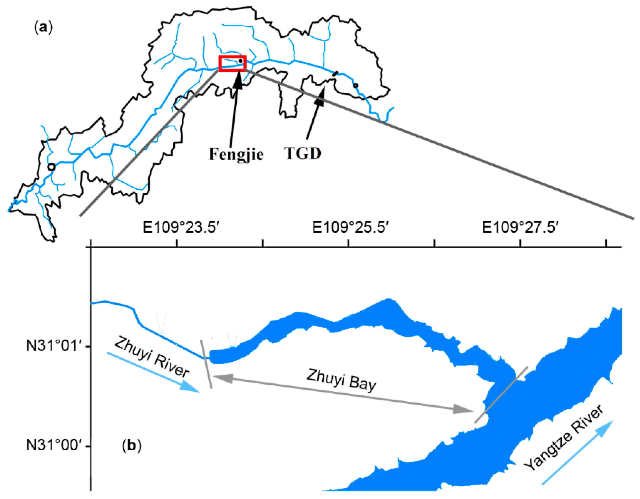
The Zhuyi River (ZR) is a primary tributary of the north bank of the Yangtze River (Figure 1), which is located in the middle of the TGR and is 156 km away from the TGD. ZR has a watershed area of 153.6 km2, a length of 31.4 km, and an annual average discharge of 2.54 m3/s which is much lower than that of the Yangtze River’s ~11,000 m3/s. After the impoundment of the TGR, a 6-km-long bay was formed, which was influenced by TGR regulation, which can modify the water level from 145 m to 175 m. Hereafter, this area is called Zhuyi Bay (ZB) in this paper. The ZB’s average depth is 36.23 m and its maximum water depth is 80 m when the TGR is at the highest level in the winter (up to 175 m). The wind over ZB is weak with an annual mean wind speed of 1.5 m/s.
2.2. Hydrodynamic Model
A three-dimensional (3D) hydrodynamic model, i.e., the Marine Environment Research and Forecasting Model (MERF) [37], was used in this study. The model used a finite-difference scheme on a staggered C-grid in the horizontal direction. In the vertical direction, the terrain-following σ-coordinate system was adopted to accurately represent both the free surface and the bottom topography. The model included baroclinic processes with complete thermodynamics and the turbulence parameterization scheme proposed by Munk and Anderson [38]. In spite of the use of the relatively simple turbulence closure scheme, the model results show the hydrodynamic model basically represented the hydrodynamic characteristics of the study area (Section 3.1) and the closure scheme was of high computational efficiency. Therefore, the turbulence parameterization scheme is deemed to be sufficient for this study. Advection terms in the model were discretized using a total variation diminishing (TVD) scheme with second-order accuracy [39]. The second-order accurate and semi-implicit scheme was employed to solve for the surface elevation. Diffusion terms are discretized using the space centered finite-difference method and solved implicitly and explicitly in the vertical and horizontal directions, respectively. The governing equations and more detailed information on the model are presented in Liu et al. [37].
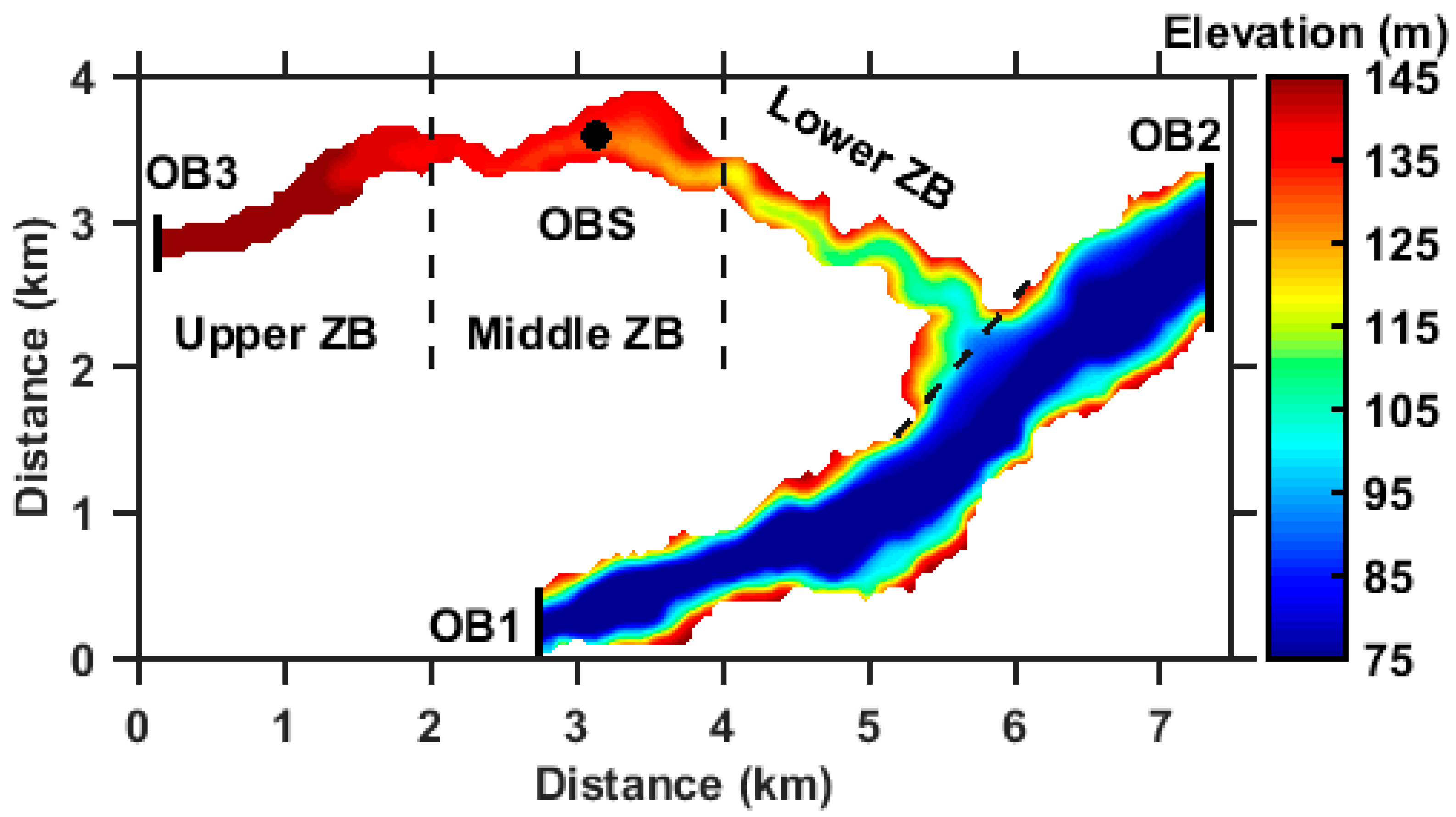
As shown in Figure 2, the model domain included the entire ZB and partial YR. The domain is discretized by 147 × 83 grids with a uniform grid spacing of 50 m. Uniform 10 σ-layers were used in the vertical direction. The time step is set to 5 s. The daily river discharge, water elevation and temperature of YR are prescribed at the boundaries OB1 and OB2 (Figure 2). The daily river discharge and water temperature of Zhuyi River in 2014 are prescribed at OB3 (Figure 2). Daily winds stress and heat flux are prescribed at the water surface. The wind stress and heat flux are calculated by bulk formulas [40]. The daily water level data were provided by the China Three Gorges Corporation. The daily meteorological data are obtained from the Fengjie Meteorological Bureau. The daily river water temperature data are interpolated from the monthly mean data. In addition, to validate the hydrodynamic model, we also conducted in situ observations at site OBS in ZB for 12 months. We measured the velocity and water temperature for one day for each month using the Nortek Velocimeter (Vector-300 m) and YSI (Yellow Springs Instruments Inc., Yellow springs, OH, USA) EXO2 multisensor sonde, respectively.
Assuming that the interannual variability of the hydrodynamics can be ignored compared to the significant seasonal cycle and the annual TGR regulation is basically similar, we regard the forcing data of 2014 as a climatological forcing to drive the model and attain the climatological hydrodynamics of ZB. After 3 years spin-up, the modeled velocity and diffusion coefficient results in one year are outputted to drive the RT model introduced in the next section.
2.3. Diagnosing RT by the Adjoint Method
In this study, the adjoint method for deriving RT developed by Delhez et al. [41] is used. The governing equation of RT derived by Delhez et al. [41] is presented below:
where denotes RT, is the velocity field, is the diffusion tensor, and is the characteristic function of the domain of interest , and . Equation (1) must be integrated backward in time with the reversed flow to solving [41].
Based on Equation (1), the RT model was established. The adjoint model is dealt with using the same finite-difference method and the same grids and layers as the hydrodynamic model. A total variation diminishing scheme with a Superbee and HSIMT (High-order Spatial Interpolation at the Middle Temporal level) alternating flux limiter (TVDal) developed by Lin and Liu is used in the advection term discretization [39]. The initial RT field is set to zero [42]. The ZB mouth connecting ZB and YR is regarded as the open boundary of the control region. The homogenous Dirichlet boundary conditions are prescribed on this boundary [42,43]. The impermeable boundary, i.e., , is used at the closed boundaries (i.e., the water-air interface, the bottom and the lateral boundaries) [41,44]. We ran the RT model backward in time using previously saved velocity and diffusion coefficients fields. The RT value in ZB reaches a stable value after 2 years spin-up, and the RT in the third year is used for analysis.
3. Results
3.1. Validation of the Hydrodynamic Model
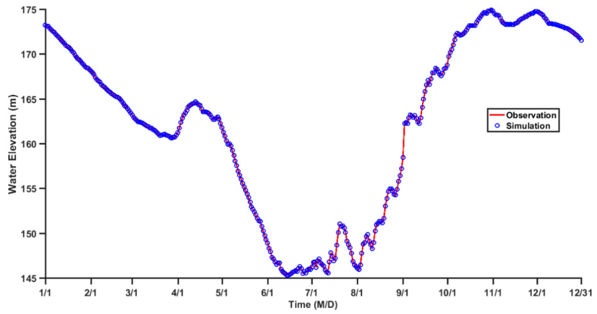
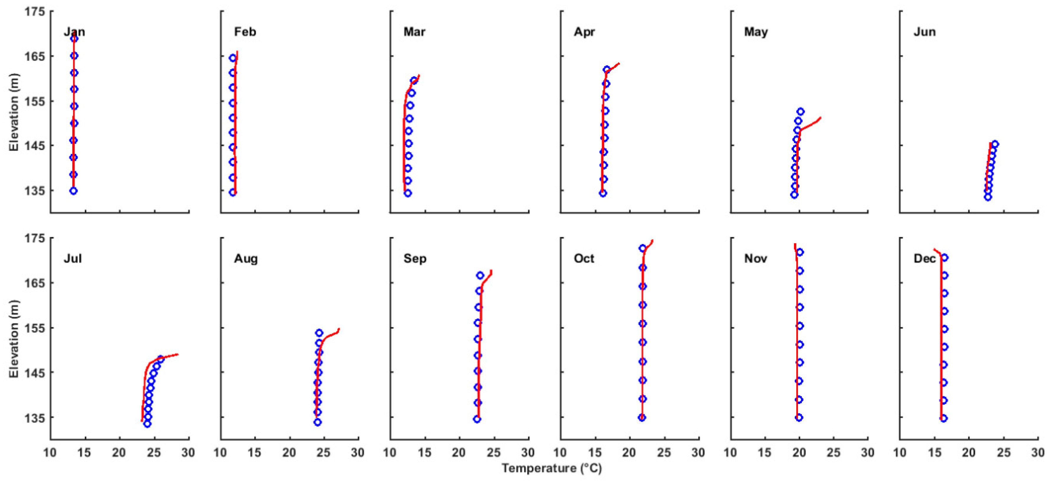
Due to the TGR regulation, the water level decreases from about 173 m elevation in January to 145 m elevation in June, remains at this level for about two months, and then increases from 145 m elevation in August to 175 m elevation in November and December. Due to the prescription on the open boundary and the fast gravity wave speed, the simulated water level change is highly consistent with the measured data, with the maximum error of less than 2 cm (Figure 3). The hydrodynamic model for ZB is further validated using observed velocity and water temperature at site OBS in ZB (Figure 2) in 2014. The simulated velocity shows a pattern of density current where the velocity directions in the upper layer and lower layer are opposite for most of the months. The magnitude of the current is basically less than 4 cm/s. The simulated flow field agrees well with the pattern of observed current (Figure 4). The observed water temperature profiles show that the water temperature in ZB increases from January to July and decreases from August to December and the annual mean difference between the surface layer and the bottom layer is ~0.2 °C (Figure 5). The monthly variation and the vertical distribution of the modeled water temperature are also consistent with the observations (Figure 5). Overall, there is a good agreement between the model results and the observations, indicating that the model used in this study can basically reproduce the main features of the hydrodynamics of ZB.
3.2. Annual Mean RT of ZB
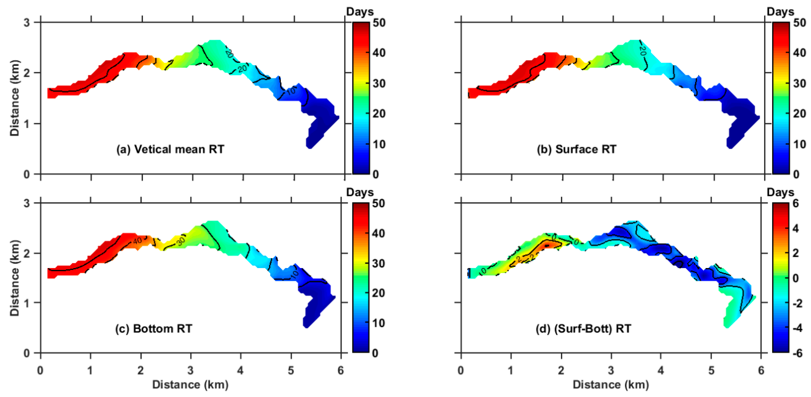
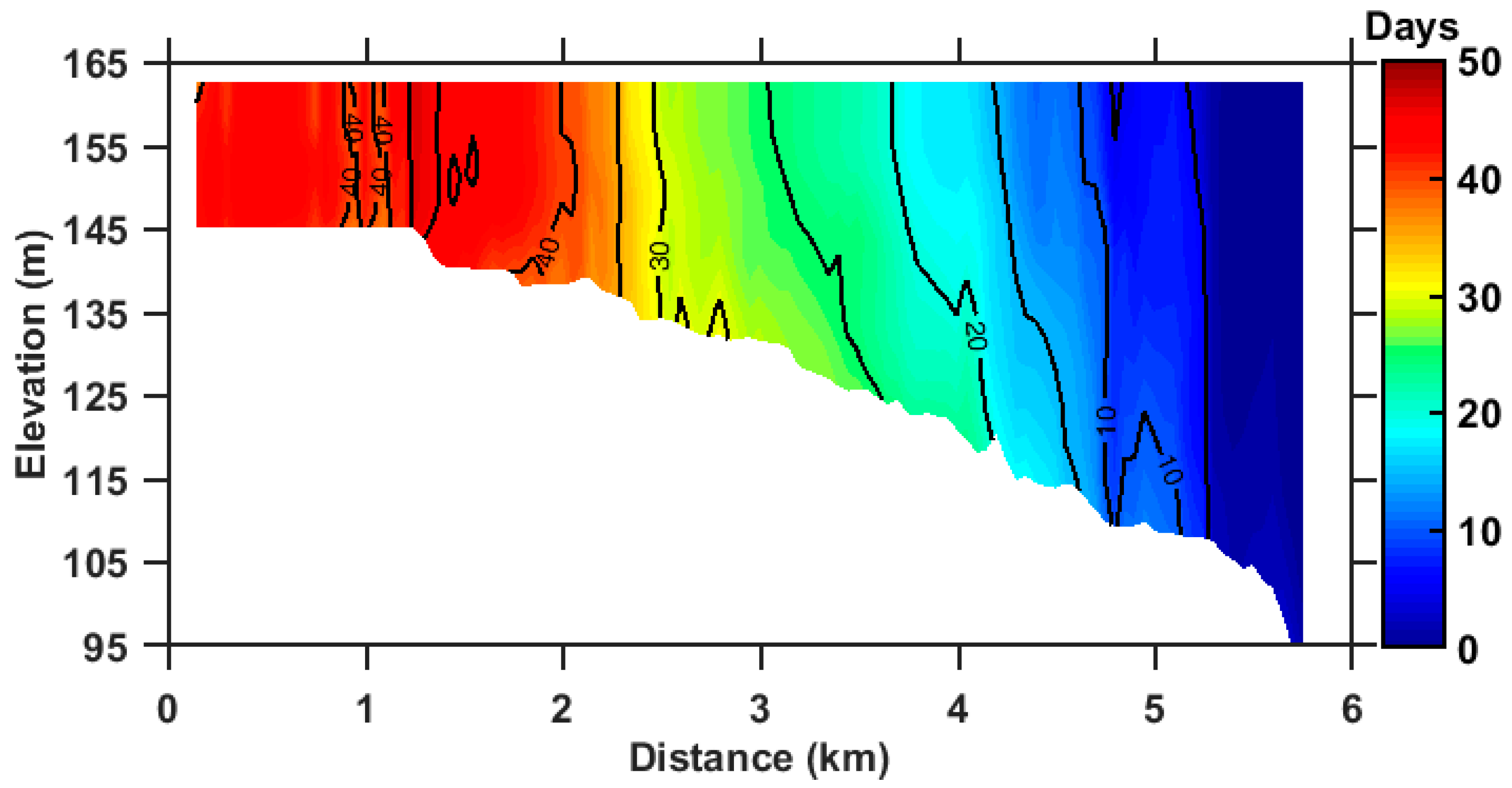
The annual mean RT of ZB is presented in Figure 6. The volume-averaged RT is 16.7 days. There is a clear longitudinal variation of RT which increases from the bay mouth to the bay top. The vertical mean RT ranges from 0 to 21 days in the lower ZB, 21 to 41 days in the middle ZB, and 41 to 53 days in the upper ZB (Figure 6a). The averaged RT of the upper, middle, and lower ZB are 37.9, 24.5, and 6.0 days, respectively. A relatively rapid spatial variation in RT occurs in the middle ZB with a relatively narrow channel. The RT distributions in the surface and bottom layers are basically consistent with the vertical mean (Figure 6b,c). The vertical difference between the surface and bottom RT was less six days in the entire ZB (Figure 6d). The mean surface RT of ZB was about 16.6 days which is slightly lower than the mean bottom RT (18.7 days). As shown in Figure 7, RT is vertically uniform along the deep channel section basically, while the surface RT was slightly larger than the bottom RT in the upper ZB, while it was reversed in the middle and lower ZB. The magnitude of current is the order of 1 cm/s. For the horizontal length of 6 km, the timescale of horizontal transport is about 69 days. The mixing coefficient is about the order of 0.003 m2/s. For the average water depth of 20 m, the timescale of vertical mixing is about 1.5 days, which is much smaller than that of the horizontal transport. Therefore, the annual mean RT exhibits little vertical variability.
3.3. Seasonal Variation of RT
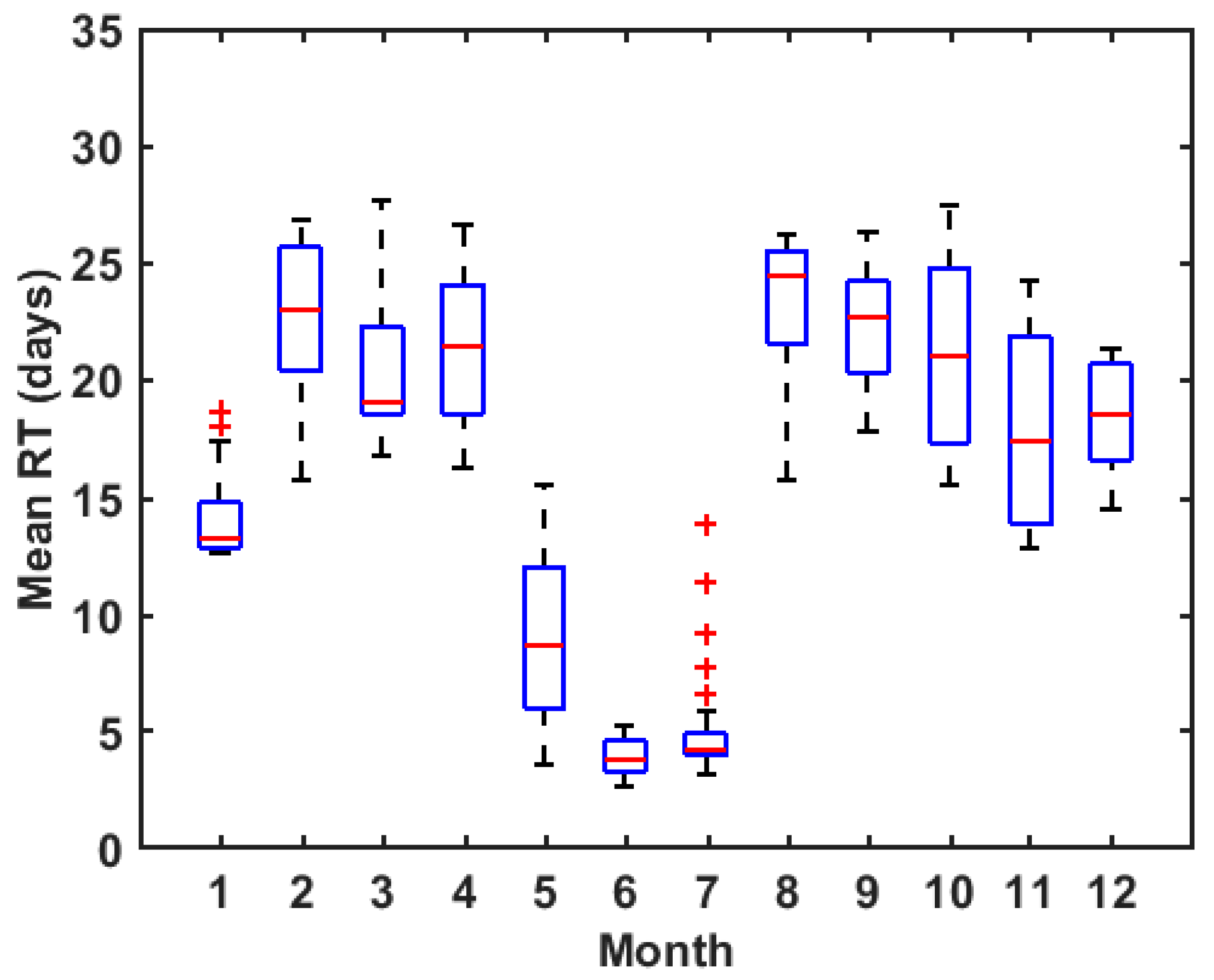
The RT of ZB exhibits a remarkable monthly variation (Figure 8). The smallest average RT value is less than 10 days which occurs in the late spring and early summer (May-July), while in other seasons, the average RT is more than 15 days. The average RT in February-April and August-October are longest which are even more than 20 days. This seasonal variation in RT implies that soluble nutrients in ZB could have a relatively short retention time in summer. In contrast, nutrient released in the spring and autumn has a longer retention time in the ZB, which could provide favorable conditions for the algae bloom in spring.
The RT variations along the bay for different months are shown in Figure 9. The RT decreases from the bay top to the bay mouth in all months. More significant monthly variation occurs at the upper ZB. In the upper ZB, the largest RT can reach more than 60 days in winter and RT in June is only 10 days. At the bay mouth, RT is basically less than 10 days for all months. In addition, there are minor vertical differences in the entire ZB, and the vertical difference is less than 10 days (results are not shown).
4. Discussion
4.1. Relationship between RT and TGR Regulation
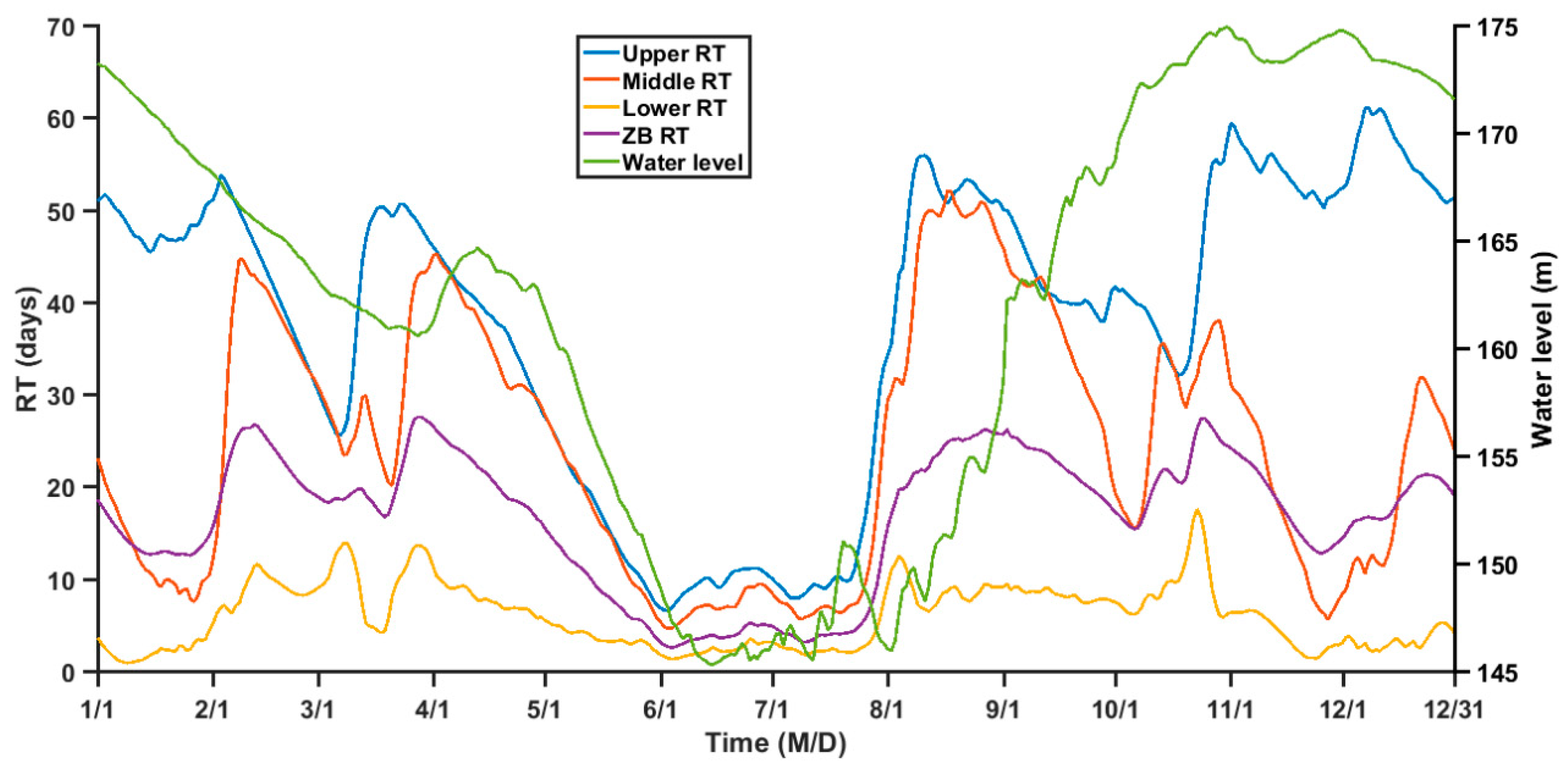
The TGR regulation changes the water level of tributary bays, which in turn influences the water depth and velocity in tributary bays. The daily variation in RT of ZB shows a good correlation to the water level (Figure 10). Therefore, it is of interest to examine the impact of TGR regulation on the RT.
As shown in Figure 10, the water level declines from January to June, remains low for two months (i.e., June and July), and elevates form August to December. A similar variation happens to the RT in ZB which decreases rapidly before June and increase after July (Figure 10). Average RT of ZB in June and July are lowest in a year, corresponding to the lowest water level in these two months. The Pearson correlation between water level and the RT of the upper, middle, lower, and ZB average is 0.735, 0.153, 0.141 and 0.552, respectively, and the correlations are all significant at the 0.01 level, indicating a significant influence of TGR regulation on the tributary bay RT, though the correlation between the water level and RT is different for different regions of ZB.
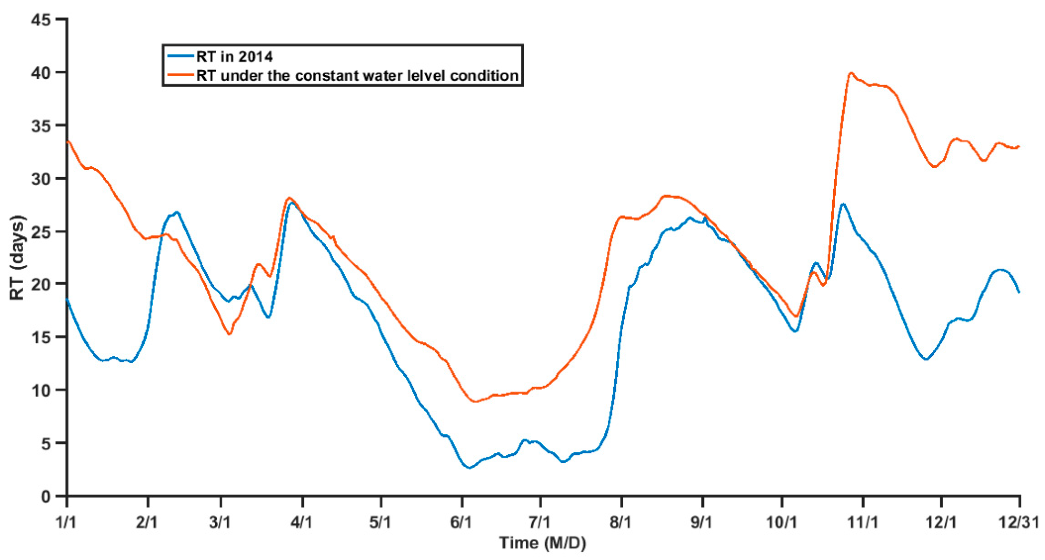
To further examine the impact of TGR regulation on the RT, a sensitivity experiment in which the water level is maintained at an annual mean level of 162.30 m is conducted. The results of the experiment show that the RT of ZB is significantly modified where the water level was maintained constant (Figure 11). The average RT in June and July increases to two times comparing to the original RT, which suggests that the low water level are favorable for the water exchange of the tributary bay while the high water level maintained by TGR could increase the water RT in the tributary bay.
In the spring and autumn, the water level of TGR is relatively high which could induce a higher RT of ZB than that of the other seasons, especially in the upper and middle reaches (Figure 9), which would result in water environment problems. Previous research has shown that the algae bloom often occurred in spring and autumn at the upper and middle reach of the tributary bay [45,46,47,48]. The high RT in this region of tributary suggested that the nutrient could have the longer retention time and could not be diluted immediately, which could be beneficial to phytoplankton growth, and algae bloom occurred as the result.
4.2. Influences of Dynamic Processes on the RT
The above analyses suggest that the water level of TGR plays an important role in the seasonal variation in the RT of ZB. To further understand the impacts of other dynamic factors on the tributary bay RT, we conducted a set of sensitivity experiments. In the experiments, we artificially modified the driving forces and calculate the RT again. Four cases (Table 1) were designed to examine the influences of driving forces, including local winds, baroclinic forcing, and river discharge on the RT. When running each of these cases, only one driving force from the control case (hereafter referred to as Case 0, whose results were presented in Section 4) is changed. In the experiment of Case 4 with no baroclinic forcing, the water temperature in the entire domain was set to be uniform and constant. The uniform and constant temperature formed a field of uniform water density, thus the baroclinic forcing is zero in Case 4. Both the hydrodynamic model and the RT model were run again to obtain a new ZB RT for each case (Table 1). The new RTs for different cases were compared to the RT of the control case to quantify the impact of different dynamic processes on the RT of ZB.
The variation of RT is generally believed to be highly related to the river discharge [49,50]. The effects of the tributary discharge and Yangtze River discharge on the RT are examined. Both the change of the tributary discharge and Yangtze River discharge account for a minor percentage of the variation of the RT (Figure 12). When the Zhuyi River discharge was decreased by 50% (Case 1), the RT in different regions increased only several days. When the Yangtze River discharge was decreased by 50% (Case 2), there was a similar pattern to Case 1. The little change of RT in Cases 1 and 2 indicate that the tributary RT is not dominated by the river discharge, which may be due to the weak discharge of the Zhuyi River and the weak impact of the Yangtze River flow on the water exchange of ZB.
The influence of wind on estuarine and semi-enclosed sea circulation has long been recognized [51,52,53]. However, the comparison between Case 3 and Case 0 suggests that the impact of winds on the tributary RT is also insignificant (Figure 12). The average speed of wind over ZB is only 1.45 m/s, which is much weaker than the wind over estuaries and semi-enclosed seas, and thus the influence of wind on tributary RT is very limited as suggested by the sensitivity experiment.
The exclusion of baroclinic forcing (Case 4) significantly increases the RT in ZB (Figure 12). Comparing to the control case, RT in the upper, middle and lower ZB increase 77.3 days, 56.2 days and 9.7 days, respectively. The average RT of ZB increases from 44% to 503%. The experiment suggests that the baroclinic current induced by the density difference is critical for the RT in ZB and thus plays a dominant role in the water exchange of ZB.
There is an apparent seasonal variation in the temperature difference between ZB and Yangtze River (Figure 13). The water temperature difference can induce the density current (see Figure 4) and enhance the water exchange between the tributary and Yangtze River. The density-induced circulation accelerated the water exchange was also found in the James River [54], the Bohai Sea [55] and the Seto Inland Sea [56]. The larger difference of water temperature in June and July could enhance the density current. The intense density current along with a smaller volume induces the lowest RT in June and July. In addition, the seasonal variation in the difference in water temperature could account for the seasonal variation in RT in ZB for the experiment with the constant water level. Therefore, the density-induced circulation is an important dynamic process for the water exchange of ZB.
4.3. The Potential Relationship between RT and Algal Blooms in the Tributary
Previous studies have shown that the algal bloom showed a longitudinal characteristic in tributary bays of TGR. Algal blooms often occurred in the upper and middle reaches of tributary bays [48,57]. The relationship between phytoplankton biomass and transport time [2] may explain this phenomenon. There is a clear longitudinal variation in RT which increases from the lower ZB to the upper ZB. The longer RT in the upper and middle bay indicates that the algal growth could be faster than the loss (i.e., transported out of the bay) in this region. By contrast, the shorter RT in the lower bay suggests that the loss may be faster than the growth and the phytoplankton biomass decreases in this region. Therefore, the possibility of algae bloom in the lower bay is very small.
In addition, previous studies also showed that the algae bloom in tributary bays of TGR often occurred in the spring and autumn [32,58] when the RT is longer and the longitudinal gradient of RT is also larger compared to summer (Figure 8). The algal growth may be faster than the loss in these months. Therefore, possibility of algae bloom in these months is relatively large. The seasonal variation in RT can provide a hydrodynamic explanation for the seasonal algal bloom. However, the mechanism of algal blooms still needs to be further investigated by means of biogeochemical analyses and phytoplankton ecosystem numerical modeling.
5. Conclusions
To understand the water exchange capacity of the tributary bay of TGR, this study investigated the spatiotemporal variation in RT in one of typical tributary bay of TGR, i.e., ZB, using the numerical simulation and the adjoint method for obtaining RT. The impacts of the water level, river discharge, wind, and baroclinic forcing on the variation of RT were further discussed based on sensitivity experiments. The main conclusions are summarized as follows. (1) The annual mean RT of ZB is 16.7 days. There were minor vertical differences (<6 days) in the entire ZB due to the water being well mixed in ZB. (2) The RT of ZB increases from the bay mouth (<5 days) to the bay top (>50 days). (3) There is a significant seasonal variation of RT, with high RT in the spring and autumn and lower RT in the summer. (4) The TGR water level regulation has a strong influence on tributary RT. The increase in the water level could increase the RT in the tributary bay. (5) The impact of the tributary discharge, the Yangtze River discharge, and wind on RT are minimal, while the baroclinic forcing induced by the temperature difference between the mainstream and tributary exerts a significant impact on RT.
Author Contributions
Conceptualization, Y.C. and L.L.; methodology, H.W. and L.L.; investigation, Z.M., F.Z. and Y.L.; writing—original draft preparation, Y.C. and L.L.
Funding
The study was financially supported by the National Key R&D Program of China (2017YFC0505305), the National Natural Science Foundation of China (51509066), the China Postdoctoral Science Foundation Funded Project (2017M621409), and the University Science and Technology Research Project of Hebei, China (ZD2019005).
Acknowledgments
The authors appreciated the editor and two anonymous reviewers for their constructive comments and suggestions on the revision of this paper.
Conflicts of Interest
The authors declare no conflict of interest.
Abbreviations
| Acronym | Full Name |
| TGR | Three Gorges Reservoir |
| TGD | Three Gorges Dam |
| ZB | Zhuyi Bay |
| RT | Residence time |
References
- De Brauwere, A.; de Brye, B.; Blaise, S.; Deleersnijder, E. Residence time, exposure time and connectivity in the Scheldt Estuary. J. Mar. Syst. 2011, 84, 85–95. [Google Scholar] [CrossRef]
- Lucas, L.V.; Thompson, J.K.; Brown, L.R. Why are diverse relationships observed between phytoplankton biomass and transport time? Limnol. Oceanogr. 2009, 54, 381–390. [Google Scholar] [CrossRef]
- McLusky, D.S.; Elliott, M.; Elliott, M. The Estuarine Ecosystem: Ecology, Threats and Management; Oxford University Press: Oxford, UK, 2004. [Google Scholar]
- Wolanski, E.; Elliott, M. Estuarine Ecohydrology: An Introduction; Elsevier: Amsterdam, The Netherlands, 2015. [Google Scholar]
- Delhez, É.J.M.; Wolk, F. Diagnosis of the transport of adsorbed material in the Scheldt Estuary: A proof of concept. J. Mar. Syst. 2013, 128, 17–26. [Google Scholar] [CrossRef]
- Andutta, F.P.; Ridd, P.V.; Deleersnijder, E.; Prandle, D. Contaminant exchange rates in estuaries—New formulae accounting for advection and dispersion. Prog. Oceanogr. 2014, 120, 139–153. [Google Scholar] [CrossRef]
- Bolin, B.; Rodhe, H. A note on the concepts of age distribution and transit time in natural reservoirs. Tellus 1973, 25, 58–62. [Google Scholar] [CrossRef]
- Zimmerman, J.T.F. Mixing and flushing of tidal embayments in the western dutch wadden sea part I: Distribution of salinity and calculation of mixing time scales. Neth. J. Sea Res. 1976, 10, 149–191. [Google Scholar] [CrossRef]
- Takeoka, H. Fundamental concepts of exchange and transport time scales in a coastal sea. Cont. Shelf Res. 1984, 3, 311–326. [Google Scholar] [CrossRef]
- Delhez, E.J.M.; Campin, J.-M.; Hirst, A.C.; Deleersnijder, E. Toward a general theory of the age in ocean modelling. Ocean Model. 1999, 1, 17–27. [Google Scholar] [CrossRef] [Green Version]
- Delhez, É.J.M. On the concept of exposure time. Cont. Shelf Res. 2013, 71, 27–36. [Google Scholar] [CrossRef]
- Nixon, S.W.; Ammerman, J.W.; Atkinson, L.P.; Berounsky, V.M.; Billen, G.; Boicourt, W.C.; Boynton, W.R.; Church, T.M.; Ditoro, D.M.; Elmgren, R.; et al. The fate of nitrogen and phosphorus at the land-sea margin of the north atlantic ocean. Biogeochemistry 1996, 35, 141–180. [Google Scholar] [CrossRef]
- Dettmann, E.H. Effect of water residence time on annual export and denitrification of nitrogen in estuaries: A model analysis. Estuaries 2001, 24, 481–490. [Google Scholar] [CrossRef]
- Crump, B.C.; Hopkinson, C.S.; Sogin, M.L.; Hobbie, J.E. Microbial biogeography along an estuarine salinity gradient: Combined influences of bacterial growth and residence time. Appl. Environ. Microbiol. 2004, 70, 1494–1505. [Google Scholar] [CrossRef]
- Delesalle, B.; Sournia, A. Residence time of water and phytoplankton biomass in coral reef lagoons. Cont. Shelf Res. 1992, 12, 939–949. [Google Scholar] [CrossRef]
- Lucas, L.V.; Koseff, J.R.; Cloern, J.E.; Monismith, S.G.; Thompson, J.K. Processes governing phytoplankton blooms in estuaries. I: The local production-loss balance. Mar. Ecol. Prog. Ser. 1999, 187, 1–15. [Google Scholar] [CrossRef]
- Lucas, L.V.; Koseff, J.R.; Monismith, S.G.; Cloern, J.E.; Thompson, J.K. Processes governing phytoplankton blooms in estuaries. II: The role of horizontal transport. Mar. Ecol. Prog. Ser. 1999, 187, 17–30. [Google Scholar] [CrossRef]
- Valiela, I.; McClelland, J.; Hauxwell, J.; Behr, P.J.; Hersh, D.; Foreman, K. Macroalgal blooms in shallow estuaries: Controls and ecophysiological and ecosystem consequences. Limnol. Oceanogr. 1997, 42, 1105–1118. [Google Scholar] [CrossRef] [Green Version]
- Chen, C.; Li, J.; Shen, H.; Wang, Z. Yangtze river of China: Historical analysis of discharge variability and sediment flux. Geomorphology 2001, 41, 77–91. [Google Scholar] [CrossRef]
- Nilsson, C.; Reidy, C.A.; Dynesius, M.; Revenga, C. Fragmentation and flow regulation of the world’s large river systems. Science 2005, 308, 405. [Google Scholar] [CrossRef]
- Yang, S.L.; Zhang, J.; Dai, S.B.; Li, M.; Xu, X.J. Effect of deposition and erosion within the main river channel and large lakes on sediment delivery to the estuary of the yangtze river. J. Geophys. Res. Earth Surf. 2007, 112, 111–119. [Google Scholar] [CrossRef]
- Wu, J.; Huang, J.; Han, X.; Xie, Z.; Gao, X. Three-gorges dam—Experiment in habitat fragmentation? Science 2003, 300, 1239–1240. [Google Scholar] [CrossRef] [PubMed]
- Shen, G.; Xie, Z. Three Gorges Project: Chance and challenge. Science 2004, 304, 681. [Google Scholar] [CrossRef]
- Stone, R. Three Gorges Dam: Into the unknown. Science 2008, 321, 628–632. [Google Scholar] [CrossRef] [PubMed]
- Fu, B.-J.; Wu, B.-F.; Lü, Y.-H.; Xu, Z.-H.; Cao, J.-H.; Niu, D.; Yang, G.-S.; Zhou, Y.-M. Three Gorges Project: Efforts and challenges for the environment. Prog. Phys. Geogr. 2010, 34, 741–754. [Google Scholar] [CrossRef]
- Xu, X.; Tan, Y.; Yang, G. Environmental impact assessments of the Three Gorges Project in China: Issues and interventions. Earth Sci. Rev. 2013, 124, 115–125. [Google Scholar] [CrossRef] [Green Version]
- Holbach, A.; Norra, S.; Wang, L.; Yijun, Y.; Hu, W.; Zheng, B.; Bi, Y. Three Gorges Reservoir: Density pump amplification of pollutant transport into tributaries. Environ. Sci. Technol. 2014, 48, 7798–7806. [Google Scholar] [CrossRef] [PubMed]
- Zhao, Y.; Zheng, B.; Wang, L.; Qin, Y.; Li, H.; Cao, W. Characterization of mixing processes in the confluence zone between the Three Gorges Reservoir mainstream and the daning river using stable isotope analysis. Environ. Sci. Technol. 2016, 50, 9907–9914. [Google Scholar] [CrossRef]
- Cheng, Y.; Wang, Y.; Zhou, H.; Dang, C. The influence of the Three Gorges Reservoir regulation on a typical tributary heat budget. Environ. Earth Sci. 2018, 77, 764. [Google Scholar] [CrossRef]
- Cheng, Y.; Wang, Y.; Zhou, H.; Hu, M.; Jiang, R.; Bao, Y.; Dang, C. Heat budget contribute rate in the Three Gorges Reservoir tributary bay between mainstream and tributary using stable isotope analysis. Water Supply 2019, 19, 553–564. [Google Scholar] [CrossRef]
- Wang, L.; Cai, Q.; Tan, L.; Kong, L. Phytoplankton development and ecological status during a cyanobacterial bloom in a tributary bay of the Three Gorges Reservoir, China. Sci. Total Environ. 2011, 409, 3820–3828. [Google Scholar] [CrossRef]
- Liu, L.; Liu, D.; Johnson, D.M.; Yi, Z.; Huang, Y. Effects of vertical mixing on phytoplankton blooms in xiangxi bay of Three Gorges Reservoir: Implications for management. Water Res. 2012, 46, 2121–2130. [Google Scholar] [CrossRef]
- Yang, Z.; Cheng, B.; Xu, Y.; Liu, D.; Ma, J.; Ji, D. Stable isotopes in water indicate sources of nutrients that drive algal blooms in the tributary bay of a subtropical reservoir. Sci. Total Environ. 2018, 634, 205–213. [Google Scholar] [CrossRef] [PubMed]
- Cheng, Y.; Li, Y.; Ji, F.; Wang, Y. Global sensitivity analysis of a water quality model in the Three Gorges Reservoir. Water 2018, 10, 153. [Google Scholar] [CrossRef]
- Zhou, Z.; Li, X.; Chen, L.; Li, B.; Liu, T.; Ai, B.; Yang, L.; Liu, B.; Chen, Q. Macrobenthic assemblage characteristics under stressed waters and ecological health assessment using ambi and m-ambi: A case study at the xin’an river estuary, yantai, China. Acta Oceanol. Sin. 2018, 37, 77–86. [Google Scholar] [CrossRef]
- Li, H.; Li, Z.; Li, Z.; Yu, J.; Liu, B. Evaluation of ecosystem services: A case study in the middle reach of the heihe river basin, northwest China. Phys. Chem. Earth Parts A/B/C 2015, 89–90, 40–45. [Google Scholar] [CrossRef]
- Liu, Z.; Lin, L.; Xie, L.; Gao, H. Partially implicit finite difference scheme for calculating dynamic pressure in a terrain-following coordinate non-hydrostatic ocean model. Ocean Model. 2016, 106, 44–57. [Google Scholar] [CrossRef]
- Munk, W.H. Note on the theory of the thermocline. J. Mar. Res. 1948, 7, 276–295. [Google Scholar]
- Lin, L.; Liu, Z. Tvdal: Total variation diminishing scheme with alternating limiters to balance numerical compression and diffusion. Ocean Model. 2019, 134, 42–50. [Google Scholar] [CrossRef]
- Fairall, C.W.; Bradley, E.F.; Rogers, D.P.; Edson, J.B.; Young, G.S. Bulk parameterization of air-sea fluxes for tropical ocean-global atmosphere coupled-ocean atmosphere response experiment. J. Geophys. Res. Oceans 1996, 101, 3747–3764. [Google Scholar] [CrossRef]
- Delhez, É.J.M.; Heemink, A.W.; Deleersnijder, É. Residence time in a semi-enclosed domain from the solution of an adjoint problem. Estuar. Coast. Shelf Sci. 2004, 61, 691–702. [Google Scholar] [CrossRef]
- Delhez, E.J.M. Transient residence and exposure times. Ocean Sci. 2006, 2, 1–9. [Google Scholar] [CrossRef] [Green Version]
- Delhez, É.J.M.; Deleersnijder, É. The boundary layer of the residence time field. Ocean Dyn. 2006, 56, 139–150. [Google Scholar] [CrossRef]
- De Brye, B.; de Brauwere, A.; Gourgue, O.; Delhez, E.J.M.; Deleersnijder, E. Water renewal timescales in the Scheldt Estuary. J. Mar. Syst. 2012, 94, 74–86. [Google Scholar] [CrossRef]
- Zeng, H.; Song, L.; Yu, Z.; Chen, H. Distribution of phytoplankton in the Three-Gorge Reservoir during rainy and dry seasons. Sci. Total Environ. 2006, 367, 999–1009. [Google Scholar] [CrossRef]
- Zhou, G.; Bi, Y.; Zhao, X.; Chen, L.; Hu, Z. Algal growth potential and nutrient limitation in spring in Three-Gorges Reservoir, China. Fresenius Environ. Bull. 2009, 18, 1642–1647. [Google Scholar]
- He, Q.; Kang, L.; Sun, X.; Jia, R.; Zhang, Y.; Ma, J.; Li, H.; Ai, H. Spatiotemporal distribution and potential risk assessment of microcystins in the Yulin River, a tributary of the Three Gorges Reservoir, China. J. Hazard. Mater. 2018, 347, 184–195. [Google Scholar] [CrossRef]
- Dai, H.; Mao, J.; Jiang, D.; Wang, L. Longitudinal hydrodynamic characteristics in reservoir tributary embayments and effects on algal blooms. PLoS ONE 2013, 8, e68186. [Google Scholar] [CrossRef]
- Hagy, J.D.; Boynton, W.R.; Sanford, L.P. Estimation of net physical transport and hydraulic residence times for a coastal plain estuary using box models. Estuaries 2000, 23, 328–340. [Google Scholar] [CrossRef]
- Shen, J.; Haas, L. Calculating age and residence time in the tidal york river using three-dimensional model experiments. Estuar. Coast. Shelf Sci. 2004, 61, 449–461. [Google Scholar] [CrossRef]
- Scully, M.E. Wind modulation of dissolved oxygen in Chesapeake Bay. Estuaries Coasts 2010, 33, 1164–1175. [Google Scholar] [CrossRef]
- Li, Y.; Li, M. Wind-driven lateral circulation in a stratified estuary and its effects on the along-channel flow. J. Geophys. Res. Oceans 2012, 117. [Google Scholar] [CrossRef] [Green Version]
- Du, J.; Shen, J. Water residence time in Chesapeake Bay for 1980–2012. J. Mar. Syst. 2016, 164, 101–111. [Google Scholar] [CrossRef]
- Shen, J.; Lin, J. Modeling study of the influences of tide and stratification on age of water in the tidal James River. Estuar. Coast. Shelf Sci. 2006, 68, 101–112. [Google Scholar] [CrossRef]
- Liu, Z.; Wang, H.; Guo, X.; Wang, Q.; Gao, H. The age of Yellow River water in the Bohai Sea. J. Geophys. Res. Oceans 2012, 117. [Google Scholar] [CrossRef] [Green Version]
- Wang, H.; Guo, X.; Liu, Z. The age of Yodo River water in the Seto Inland Sea. J. Mar. Syst. 2019, 191, 24–37. [Google Scholar] [CrossRef]
- Li, J.; Yang, W.; Li, W.; Mu, L.; Jin, Z. Coupled hydrodynamic and water quality simulation of algal bloom in the Three Gorges Reservoir, China. Ecol. Eng. 2018, 119, 97–108. [Google Scholar] [CrossRef]
- Ye, L.; Han, X.; Xu, Y.; Cai, Q. Spatial analysis for spring bloom and nutrient limitation in xiangxi bay of Three Gorges Reservoir. Environ. Monit. Assess. 2007, 127, 135–145. [Google Scholar] [CrossRef] [PubMed]
Figure 1.
Illustration of the domain of interest, with (a) the Yangtze River basin. (b) the location of the Zhuyi Bay (ZB).
Figure 1.
Illustration of the domain of interest, with (a) the Yangtze River basin. (b) the location of the Zhuyi Bay (ZB).

Figure 2.
Computational domain and the river elevation (m).

Figure 3.
The observed and simulated daily water level at site OBS in 2014.

Figure 4.
Comparison of the observed and simulated velocity profiles at site OBS for the 12 months in 2014. Blue circles denote simulation, and red circles denote observation.
Figure 4.
Comparison of the observed and simulated velocity profiles at site OBS for the 12 months in 2014. Blue circles denote simulation, and red circles denote observation.

Figure 5.
Comparison of observed and simulated water temperature profiles at site OBS for the 12 months in 2014. Blue circles denote simulation, and red lines denote observation.
Figure 5.
Comparison of observed and simulated water temperature profiles at site OBS for the 12 months in 2014. Blue circles denote simulation, and red lines denote observation.

Figure 6.
Vertical mean (a), surface (b), and bottom (c) RT (days) averaged over 2014. The contour interval is five days. (d) difference between the surface and bottom RT. Positive value denotes larger RT in surface layers. The contour interval is two days.
Figure 6.
Vertical mean (a), surface (b), and bottom (c) RT (days) averaged over 2014. The contour interval is five days. (d) difference between the surface and bottom RT. Positive value denotes larger RT in surface layers. The contour interval is two days.

Figure 7.
Vertical profile of the annual mean RT (days) along the deep channel section. The contour interval is five days.
Figure 7.
Vertical profile of the annual mean RT (days) along the deep channel section. The contour interval is five days.

Figure 8.
Monthly variation of RT averaged over the entire Bay. Red lines denote medians of RT in the month, blue rectangles denote the first and third quartiles, dashed lines denote the upper and lower whiskers, and red crosses denote the outliers.
Figure 8.
Monthly variation of RT averaged over the entire Bay. Red lines denote medians of RT in the month, blue rectangles denote the first and third quartiles, dashed lines denote the upper and lower whiskers, and red crosses denote the outliers.

Figure 9.
Vertical mean RT (days) averaged of each month, the contour interval is five days.

Figure 10.
Time series of daily mean RT in different ZB regions and the daily water level.

Figure 11.
Comparison of ZB RT in 2014 and RT under the constant water level.

Figure 12.
Time series of vertical mean RT in different cases.

Figure 13.
The observed water temperature difference between ZB and the Yangtze River. Positive value indicates that ZB temperature is higher than the Yangtze River. Negative value indicates that ZR temperature is lower than the Yangtze River.
Figure 13.
The observed water temperature difference between ZB and the Yangtze River. Positive value indicates that ZB temperature is higher than the Yangtze River. Negative value indicates that ZR temperature is lower than the Yangtze River.


Table 1.
Configurations of sensitivity experiments for Case 0 to Case 4.
| Case | Tributary Discharge | Yangtze River Discharge | Local Winds | Baroclinic Forcing |
|---|---|---|---|---|
| 0 | Yes | Yes | Yes | Yes |
| 1 | 0.5 times | Yes | Yes | Yes |
| 2 | Yes | 0.5 times | Yes | Yes |
| 3 | Yes | Yes | No | Yes |
| 4 | Yes | Yes | Yes | No |
© 2019 by the authors. Licensee MDPI, Basel, Switzerland. This article is an open access article distributed under the terms and conditions of the Creative Commons Attribution (CC BY) license (http://creativecommons.org/licenses/by/4.0/).
Share and Cite
MDPI and ACS Style
Cheng, Y.; Mu, Z.; Wang, H.; Zhao, F.; Li, Y.; Lin, L. Water Residence Time in a Typical Tributary Bay of the Three Gorges Reservoir. Water 2019, 11, 1585. https://doi.org/10.3390/w11081585
AMA Style
Cheng Y, Mu Z, Wang H, Zhao F, Li Y, Lin L. Water Residence Time in a Typical Tributary Bay of the Three Gorges Reservoir. Water. 2019; 11(8):1585. https://doi.org/10.3390/w11081585
Chicago/Turabian StyleCheng, Yao, Zheng Mu, Haiyan Wang, Fengxia Zhao, Yu Li, and Lei Lin. 2019. "Water Residence Time in a Typical Tributary Bay of the Three Gorges Reservoir" Water 11, no. 8: 1585. https://doi.org/10.3390/w11081585
Note that from the first issue of 2016, this journal uses article numbers instead of page numbers. See further details here.