The Development of a Calculation Model for the Instantaneous Pressure Head of Oscillating Water Flow in a Pipeline

Abstract

Sinusoidal oscillating water flow at low pressure can improve the anti-clogging ability of an emitter in drip irrigation or the water distribution of a nozzle in sprinkler irrigation and reduce the cost and energy consumption of the irrigation system. In this study, the characteristics of instantaneous pressure head attenuation of oscillating water flow along a pipeline have been investigated. By using a complex function to solve the continuity equation and the momentum equation of a pipeline with water hammer motion and using the Darcy–Weisbach formula to estimate the head loss, a calculation model for the instantaneous pressure head of oscillating water flow along a pipeline was developed. The measured value of the amplitude of the pressure head and the average instantaneous pressure head in the experiments have been used to verify the corresponding pressure head calculated by the model. The results show that the amplitude of the pressure head and the average instantaneous pressure head decrease linearly along the pipeline. The calculated value of the amplitude of the pressure head and the average instantaneous pressure head are basically close to the corresponding measured pressure head. From the results of all the tests, the maximum relative error of the calculated and measured value of the amplitude of the pressure head along the pipeline was 9.44%. The maximum relative error of the calculated and measured value of the average instantaneous pressure head along the pipeline was 8.37%. Hence, the model can accurately predict the instantaneous pressure head of oscillating water flow along a pipe and provide a theoretical basis for the application of oscillating water flow in irrigation systems and the design of irrigation pipe networks.

1. Introduction

An irrigation system with high operating pressure can mean a better water supply facility, but both the cost and the energy consumption are high. Therefore, reducing the operating pressure of an irrigation system can effectively reduce the cost and the energy consumption of the irrigation system. Such an irrigation system can be widely used in underdeveloped areas and in areas with inadequate water supply facilities. Hence, it is an important development in water-saving irrigation technology [1,2,3,4,5]. Low-pressure drip irrigation can ensure good quality irrigation and decrease cost and energy consumption; however, low operating pressure produces slower flow velocity through the drip capillarity and emitter. The slower flow velocity produces slower vortex movement in the flow passage. Hence, the emitter is more prone to clogging, which reduces the efficiency and working life of the emitter and increases the maintenance cost of the irrigation system. If an emitter is clogged, it also reduces the uniformity of irrigation, which makes the application and development of low-pressure drip irrigation and subsurface drip irrigation more challenging [6,7,8,9]. Further, for a sprinkler irrigation system with low operating pressure, the spraying range of the sprinklers for irrigation is shorter, thereby resulting in an uneven water distribution, and a higher peak sprinkler intensity. As such, it is difficult to ensure the quality of the irrigation spray is good [10,11].

In order to solve the problem of clogging in an emitter, earlier studies conducted experiments to investigate the influence of flow passage geometry parameters on the hydraulic characteristics of the emitter. Based on the experimental results, the flow passage of the emitter was optimized so as to improve the anti-clogging performance of the emitter under low pressure [12,13,14,15]. In order to improve the spraying effect of the sprinklers under low pressure, auxiliary sprinklers, jet devices, and water dispersing devices can be added or the original sprinklers can be replaced with non-circular sprinklers [16,17,18]. All these methods can improve an irrigation system so that it can operate at low pressure. But this is sometimes affected by financial considerations, and the improvements that can be gained by using these methods are also very limited.

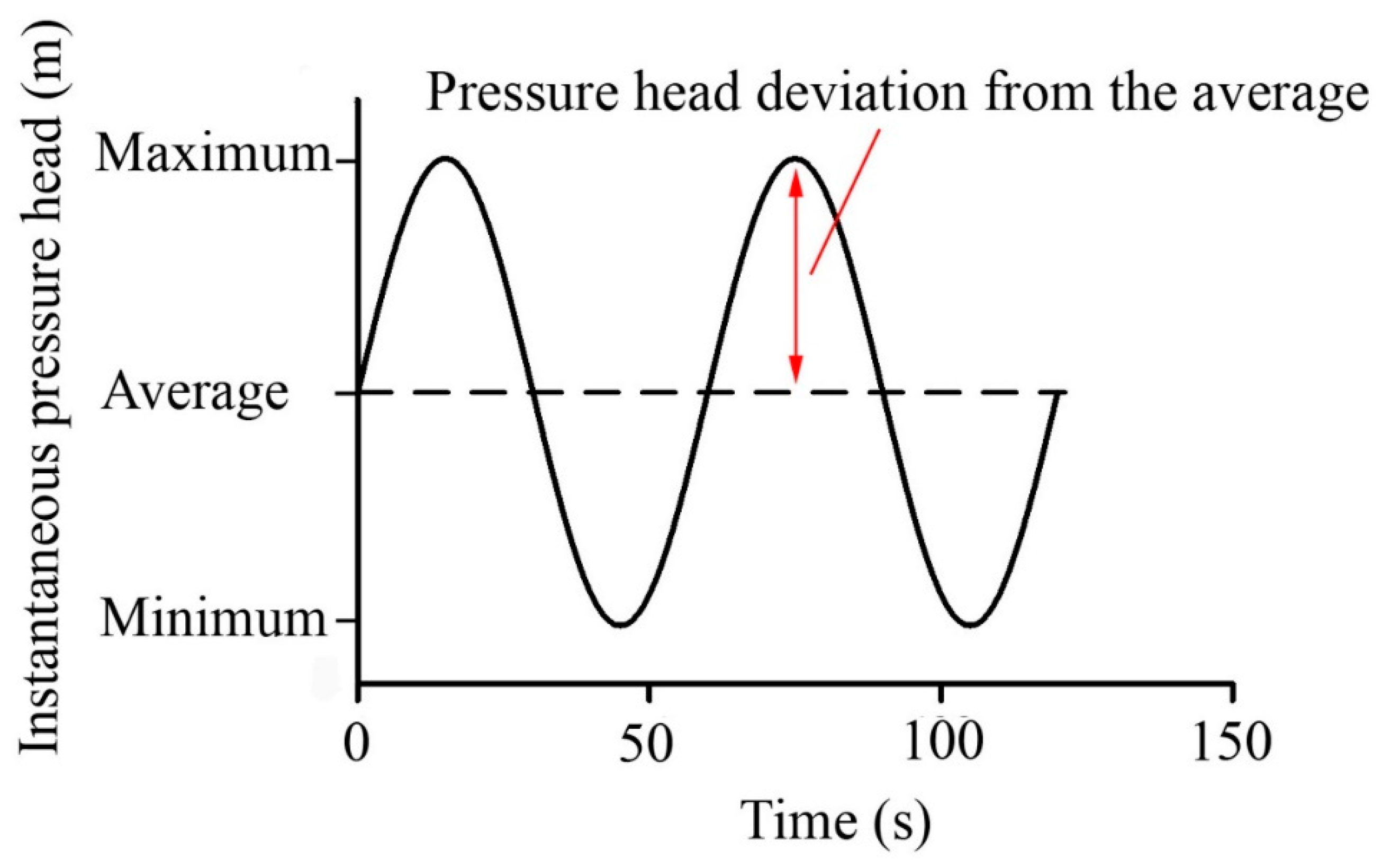
Historically, irrigation systems have always used constant water pressure. In recent years, oscillating pressure has been used in irrigation systems, which provides a new way to solve the problems in irrigation. Oscillating pressure increases the flow turbulence in an emitter, which improves the ability of the flow to transport particles, and significantly improves the anti-clogging performance of the emitter [19,20,21]. The low sinusoidal oscillating pressure can improve the intensity distribution of the sprinkler under low pressure thereby improving the economic benefit of the irrigation system. Sprinkler irrigation that uses oscillating pressure shows a good prospect in reducing soil erosion caused by runoff and salt and nutrient leaching and improving water utilization efficiency [22,23,24,25]. Oscillating water flow belongs to unsteady flow, and the studies of unsteady flow are mostly related to the water hammer motion generated by the rapid change of water flow in hydropower stations, pumping stations, and other systems [26,27,28,29,30]. Unlike the water hammer instantaneous pressure head, which fluctuates irregularly with time, the instantaneous pressure head of oscillating water flow fluctuates like a sine wave. The instantaneous pressure head in a pipeline fluctuates periodically with time, and the maximum, average, and minimum instantaneous pressures are constants. The instantaneous pressure head is formed by the superposition of the average instantaneous pressure head and the pressure head deviation from the average, as shown in Figure 1. The relationship between the instantaneous discharge of oscillating water flow and time is similar to that between the instantaneous pressure head of oscillating water flow and time.

At present, most of the studies on oscillating water flow focus on improving the clogging resistance of emitters and improving the sprinkler intensity distribution, but studies on the temporal and spatial variations of the instantaneous pressure head of oscillating water flow along a pipeline have not been reported. For this reason, the characteristics of the instantaneous pressure head of oscillating water flow changing with time was analyzed, for the first time, in this study. This was done by using a complex function to solve the continuity equation and momentum equation for the water hammer motion in a pipeline. It also uses the Darcy–Weisbach formula to estimate the head loss. The calculation model of the instantaneous pressure head of oscillating water flow along a pipeline was developed. The accuracy of the calculation model was verified with experimental data. Hence, the model can provide a theoretical basis for the application of oscillating water flow in irrigation systems and the design of irrigation pipe networks.

2. Materials and Methods

2.1. Experiments

2.1.1. Experimental Equipment and Procedure

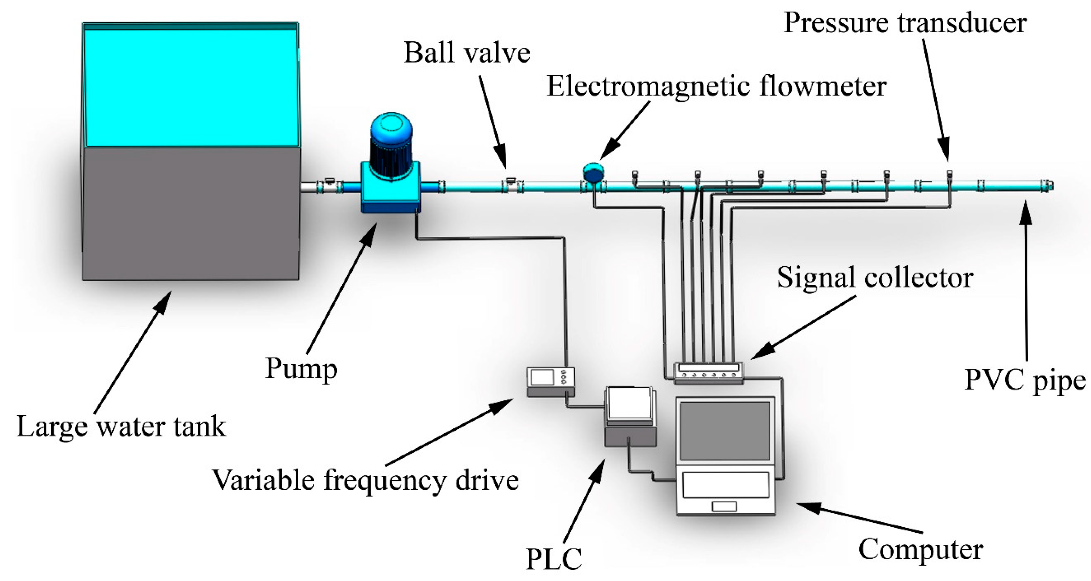
The experiments were conducted at the Irrigation Hydraulics Laboratory, Northwest A&F University, Yangling, China. The main components of the oscillating water flow pressure head test system are the PVC pipes, water tank, pump, variable frequency drive, computer, pressure transducer (range 0–0.6 MPa, accuracy 0.1%), and electromagnetic flowmeter (range 0.29–28.95 m³/h). The oscillating water pressure was produced by an automatic pressure control system that consists of a centrifugal pump with an electric motor, a variable-frequency drive (VFD), and a programmable logic controller (PLC). The experimental procedure is as follows. First, the program for implementing the designed oscillating pressure is uploaded to the PLC to control the VFD, which modifies the pump motor speed. The maximum, average, and minimum of the instantaneous pressure heads and the period of the oscillating water flow are set in the program. Second, the electric motor speed of the centrifugal pump is controlled by the VFD to produce the designed oscillating pressure. The pressure signal and flow signal are recorded by the PC equipped with the signal collector. Figure 2 shows a schematic diagram of the test platform for measuring the pressure head of the oscillating water flow.

2.1.2. Experimental Setup

The length of the PVC pipe was 60 m, the wall thickness of the pipe was 0.002 m, and the inside diameter of the pipeline was 0.036 m. A pressure transducer was installed every 12 m along the pipe. Three cases (i.e., Case D1, Case D2, and Case D3) were tested in the oscillating water flow tests.

Table 1. Parameters for the oscillating water flow tests.

Case	Average Pressure Head (m)	Amplitude of Pressure Head (m)	Average Discharge (m3/h)	Amplitude of Discharge (m3/h)	Period (s)
D1	16	8	5.71	1.56	40
D2	10	6	4.33	1.51	60
D3	8	2	4.02	0.52	80

shows the parameters for the oscillating water flow tests.

2.2. Calculation Model

As shown in Figure 1, the instantaneous pressure head and discharge of oscillating water flow can be expressed as [19,31]:

$$\mathrm{H}=\overline{\mathrm{H}}+\mathrm{h},$$

(1)

$$\mathrm{Q}=\overline{\mathrm{Q}}+\mathrm{q},$$

(2)

where H is the instantaneous pressure head (m); $\overline{\mathrm{H}}$ is the average instantaneous pressure head (m); h is the pressure head deviation from the average (m); Q is the instantaneous discharge (m³/s); $\overline{\mathrm{Q}}$ is the average instantaneous discharge (m³/s); and q is the discharge deviation from the average (m³/s).

The instantaneous pressure head and discharge fluctuations can be expressed in terms of a sine function, as follows:

$$\mathrm{h}={\mathrm{h}}^{*}\sin \left(\mathsf{\omega }\mathrm{t}\right),$$

(3)

$$\mathrm{q}={\mathrm{q}}^{*}\sin \left(\mathsf{\omega }\mathrm{t}\right),$$

(4)

where ${\mathrm{h}}^{*}$ is the amplitude of the pressure head (m); ${\mathrm{q}}^{*}$ is the amplitude of discharge (m³/s); ω is the frequency of the oscillating water flow (rad/s), and t is time (s). Further, ω is related to T, as follows:

$$\mathsf{\omega }=\frac{2\mathsf{\pi }}{\mathrm{T}},$$

(5)

where T is the period of the oscillating water flow (s). The maximum instantaneous pressure head and discharge can be obtained by substituting $\sin \left(\mathsf{\omega }\mathrm{t}\right)=1$ into Equations (3) and (4), and then substituting the corresponding h and q into Equations (1) and (2), respectively. Similarly, the minimum instantaneous pressure head and discharge can be obtained by substituting $\sin \left(\mathsf{\omega }\mathrm{t}\right)=-1$ into Equations (3) and (4), and then substituting the corresponding h and q into Equations (1) and (2), respectively.

According to Equations (1)–(4), both the instantaneous pressure head and the discharge of oscillating water flow comprise a term for steady flow and an addition term for unsteady flow. The instantaneous pressure head and discharge of oscillating water flow for the steady flow term is the average instantaneous pressure head and discharge. The unsteady flow term is the product of the amplitude of the pressure head, the amplitude of discharge, and the sine function. Therefore, in the calculation model, the instantaneous pressure head of oscillating water flow can be calculated from the amplitude of the pressure head and average instantaneous pressure head.

2.2.1. The Calculation of the Amplitude of the Pressure Head

The continuity equation and the momentum equation for water hammer motion are as follows [32]:

$$\mathrm{Momentum}\mathrm{equation}:\frac{\partial \mathrm{H}}{\partial \mathrm{x}}+\frac{1}{\mathrm{gA}}\frac{\partial \mathrm{Q}}{\partial \mathrm{t}}+\frac{{\mathrm{fQ}}^{\mathrm{n}}}{2{\mathrm{gDA}}^{\mathrm{n}}}=0,$$

(6)

$$\mathrm{Continuity}\mathrm{equation}:\frac{\partial \mathrm{Q}}{\partial \mathrm{x}}+\frac{\mathrm{gA}}{{\mathrm{a}}^2}\frac{\partial \mathrm{H}}{\partial \mathrm{t}}=0,$$

(7)

where A is the cross-sectional area of the flow in the pipe (m²); g is the acceleration due to gravity (9.8 m/s²); D is the inside diameter of the pipe (m); f is the Darcy–Weisbach friction factor; a is the wave speed (m/s); n is the exponent of the flow velocity in the friction-loss term; x is the distance along the pipeline in the direction of flow (m); and t is time (s). The wave speed, a, and the Darcy–Weisbach friction factor, f, can be calculated as follows [33,34,35]:

$$\mathrm{a}=\frac{\sqrt{\frac{\mathsf{\beta }}{\mathsf{\rho }}}}{\sqrt{1+\frac{2r\mathsf{\beta }}{\mathsf{\delta }\mathrm{E}}}},$$

(8)

$$\mathrm{f}=\frac{0.3164}{{\mathrm{R}}_{\mathrm{e}}{}^{0.25}},$$

(9)

$${\mathrm{R}}_{\mathrm{e}}=\frac{\mathrm{vD}}{\mathsf{\upsilon }}=\frac{2\overline{\mathrm{Q}}}{\mathsf{\pi }\mathrm{r}\mathsf{\upsilon }},$$

(10)

where $\mathsf{\beta }$ is the equivalent bulk modulus of water ($2.19\times {10}^9\mathrm{N}/{\mathrm{m}}^2$); $\mathsf{\rho }$ is the density of water (1000 $\mathrm{kg}/{\mathrm{m}}^3$); $\mathrm{r}$ is the inner radius of the pipe (m); $\mathsf{\delta }$ is the thickness of the pipe wall (m); $\mathrm{E}$ is the modulus of elasticity of the pipe material ($2.6\times {10}^9 \mathrm{N}/{\mathrm{m}}^2$); ${\mathrm{R}}_{\mathrm{e}}$ is the Reynolds number of the average instantaneous pressure discharge, $\mathrm{v}$ is the flow velocity in the pipe (m/s), and $\mathsf{\upsilon }$ is the kinematic viscosity of water ($1.01\times {10}^{-6} {\mathrm{m}}^2/\mathrm{s}$).

Since the average instantaneous discharge and pressure head are time invariant, and the average instantaneous discharge is constant along the length of the pipeline, $\frac{\partial \overline{\mathrm{Q}}}{\partial \mathrm{t}}$= $\frac{\partial \overline{\mathrm{H}}}{\partial \mathrm{t}}$= $\frac{\partial \overline{\mathrm{Q}}}{\partial \mathrm{x}}$ = 0. Further,

$$\frac{\partial \mathrm{Q}}{\partial \mathrm{t}}=\frac{\partial \mathrm{q}}{\partial \mathrm{t}} \frac{\partial \mathrm{Q}}{\partial \mathrm{x}}=\frac{\partial \mathrm{q}}{\partial \mathrm{x}} \frac{\partial \mathrm{H}}{\partial \mathrm{t}}=\frac{\partial \mathrm{h}}{\partial \mathrm{t}}$$

(11)

and

$$\frac{\partial \mathrm{H}}{\partial \mathrm{x}}=\frac{\partial \overline{\mathrm{H}}}{\partial \mathrm{x}}+\frac{\partial \mathrm{h}}{\partial \mathrm{x}},$$

(12)

$$\frac{\partial \overline{\mathrm{H}}}{\partial \mathrm{x}}=-\frac{{\mathrm{f}\overline{\mathrm{Q}}}^{\mathrm{n}}}{2{\mathrm{gDA}}^{\mathrm{n}}}.$$

(13)

The friction term in Equation (6) can be written as:

$$\frac{{\mathrm{fQ}}^{\mathrm{n}}}{2{\mathrm{gDA}}^{\mathrm{n}}}=\frac{\mathrm{f}{\left(\overline{\mathrm{Q}}+\mathrm{q}\right)}^{\mathrm{n}}}{2{\mathrm{gDA}}^{\mathrm{n}}}\approx \frac{{\mathrm{f}\overline{\mathrm{Q}}}^{\mathrm{n}}}{2{\mathrm{gDA}}^{\mathrm{n}}}+\frac{{\mathrm{nf}\overline{\mathrm{Q}}}^{\mathrm{n}-1}}{2{\mathrm{gDA}}^{\mathrm{n}}}\mathrm{q}+\dots$$

(14)

where, since $\mathrm{q}\langle \overline{\mathrm{Q}}$, the series in Equation (14) converges, the higher-order terms can be omitted.

On the other hand, since the friction loss is considered, substituting Equations (11)–(14) into Equations (6) and (7) can linearize the friction loss. Hence, with the linearized friction loss, Equations (6) and (7) become:

$$\frac{\partial \mathrm{h}}{\partial \mathrm{x}}+\frac{1}{\mathrm{gA}}\frac{\partial \mathrm{q}}{\partial \mathrm{t}}+\mathrm{Rq}=0,$$

(15)

$$\frac{\partial \mathrm{q}}{\partial \mathrm{x}}+\frac{\mathrm{gA}}{{\mathrm{a}}^2}\frac{\partial \mathrm{h}}{\partial \mathrm{t}}=0,$$

(16)

where $\mathrm{R}$ is the linearization resistance per unit length of the pipe, which can be expressed as follows [36]:

$$\mathrm{R}=\frac{\mathrm{f}\overline{\mathrm{Q}}}{{\mathrm{gDA}}^2}.$$

(17)

The separation of variables method can be used to solve the linearized equations (Equations (15) and (16)) by taking the partial derivatives. By canceling h and q, Equations (15) and (16) become:

$$\frac{{\partial }^2\mathrm{h}}{\partial {\mathrm{x}}^2}=\frac{1}{{\mathrm{a}}^2}\frac{{\partial }^2\mathrm{h}}{\partial {\mathrm{t}}^2}+\frac{\mathrm{f}\overline{\mathrm{Q}}}{{\mathrm{a}}^2\mathrm{D}\mathrm{A}}\frac{\partial \mathrm{h}}{\partial \mathrm{t}},$$

(18)

$$\frac{{\partial }^2\mathrm{q}}{\partial {\mathrm{x}}^2}=\frac{1}{{\mathrm{a}}^2}\frac{{\partial }^2\mathrm{q}}{\partial {\mathrm{t}}^2}+\frac{\mathrm{f}\overline{\mathrm{Q}}}{{\mathrm{a}}^2\mathrm{DA}}\frac{\partial \mathrm{q}}{\partial \mathrm{t}}.$$

(19)

The solutions of Equations (18) and (19) are as follows [37]:

$$\mathrm{h}={\mathrm{e}}^{\mathrm{st}}\left({\mathrm{C}}_1{\mathrm{e}}^{\mathsf{\mu }\mathrm{x}}+{\mathrm{C}}_2{}^{-\mathsf{\mu }\mathrm{x}}\right),$$

(20)

$$\mathrm{q}=-\frac{\mathrm{gAs}}{{\mathrm{a}}^2\mathsf{\mu }}{\mathrm{e}}^{\mathrm{st}}\left({\mathrm{C}}_1{\mathrm{e}}^{\mathsf{\mu }\mathrm{x}}-{\mathrm{C}}_2{}^{-\mathsf{\mu }\mathrm{x}}\right),$$

(21)

where

$$\mathrm{s}=\mathrm{i}\mathsf{\omega },$$

(22)

$$\mathsf{\mu }=\sqrt{-\frac{{\mathsf{\omega }}^2}{{\mathrm{a}}^2}+\frac{\mathrm{gA}\mathsf{\omega }\mathrm{Ri}}{{\mathrm{a}}^2}}.$$

(23)

The pressure head and discharge deviation from the average are both functions of position x and time t. In oscillating water flow, the pressure head and discharge deviation from the average are very close to or completely the same as the sine function with time as the independent variable. Therefore, the pressure head and discharge deviation from the average can be expressed in the form of complex functions, as follows:

$$\mathrm{h}={\mathrm{h}}^{*}\left(\mathrm{x}\right){\mathrm{e}}^{\mathsf{\omega }\mathrm{ti}},$$

(24)

$$\mathrm{q}={\mathrm{q}}^{*}\left(\mathrm{x}\right){\mathrm{e}}^{\mathsf{\omega }\mathrm{ti}},$$

(25)

where i is the imaginary unit, i.e., $\mathrm{i}=\sqrt{-1}$; ${\mathrm{h}}^{*}\left(\mathrm{x}\right)$ and ${\mathrm{q}}^{*}\left(\mathrm{x}\right)$ are the complex functions of x.

Substituting Equations (24) and (25) into Equations (20) and (21) gives:

$${\mathrm{h}}^{*}\left(\mathrm{x}\right)={\mathrm{C}}_1{\mathrm{e}}^{\mathsf{\mu }\mathrm{x}}+{\mathrm{C}}_2{\mathrm{e}}^{-\mathsf{\mu }\mathrm{x}},$$

(26)

$${\mathrm{q}}^{*}\left(\mathrm{x}\right)=-\frac{\mathsf{\omega }\mathrm{gAi}}{{\mathsf{\mu }\mathrm{a}}^2}\left({\mathrm{C}}_1{\mathrm{e}}^{\mathsf{\mu }\mathrm{x}}-{\mathrm{C}}_2{\mathrm{e}}^{-\mathsf{\mu }\mathrm{x}}\right).$$

(27)

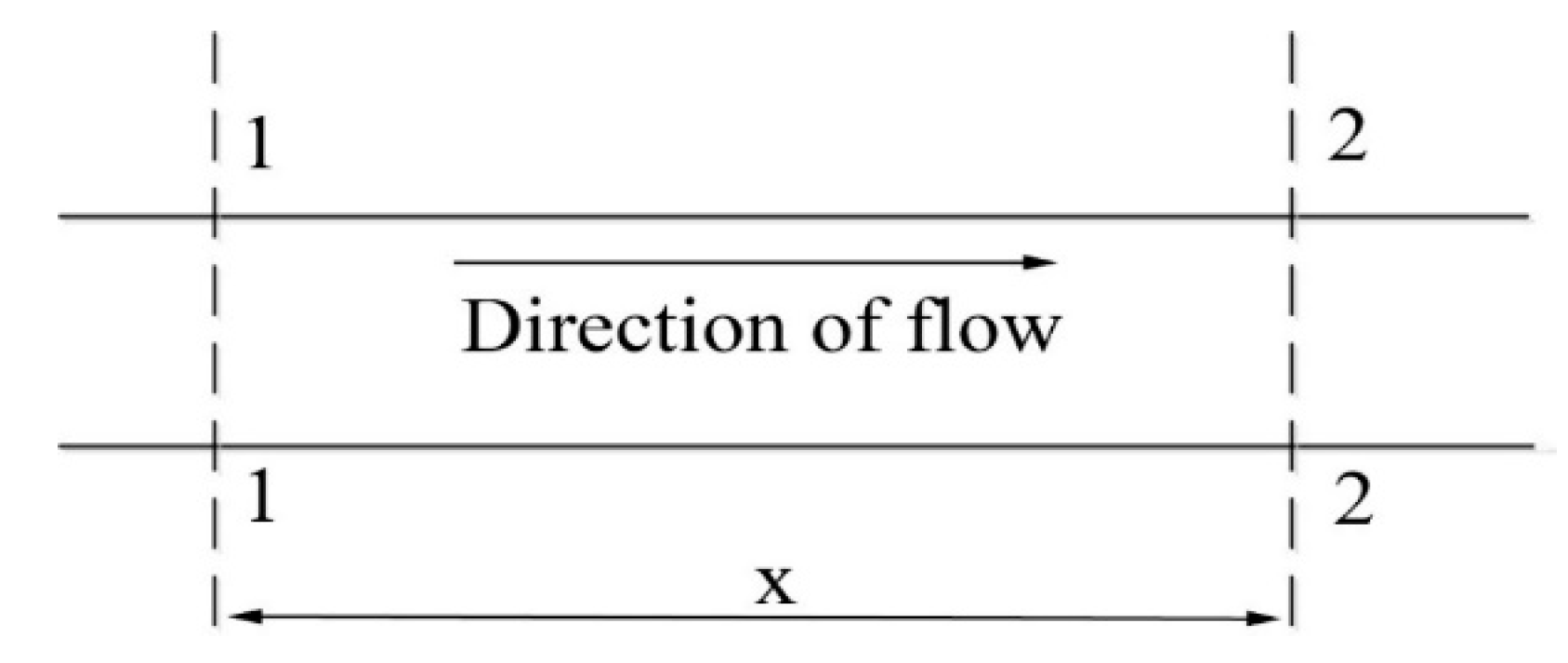
As shown in Figure 3, cross-section 1–1 and cross-section 2–2 are any two cross-sections along the pipeline. Water flows from cross-section 1–1 to cross-section 2–2. According to the pressure head and discharge at cross-section 1–1, the integral constants C₁ and C₂ can be written as:

$${\mathrm{C}}_1=\frac{1}{2}\left({\mathrm{h}}_1^{*}-\frac{{\mathsf{\mu }\mathrm{a}}^2}{\mathsf{\omega }\mathrm{gAi}}{\mathrm{q}}_1^{*}\right),$$

(28)

$${\mathrm{C}}_2=\frac{1}{2}\left({\mathrm{h}}_1^{*}+\frac{{\mathsf{\mu }\mathrm{a}}^2}{\mathsf{\omega }\mathrm{gAi}}{\mathrm{q}}_1^{*}\right),$$

(29)

where ${\mathrm{h}}_1{}^{*}$ is the amplitude of the pressure head at cross-section 1–1 (m); and ${\mathrm{q}}_1{}^{*}$ is the amplitude of discharge at cross-section 1–1 (m³/s).

Substituting Equations (28) and (29) into Equations (26) and (27) and introducing the hyperbolic function, the solutions for the amplitudes of the pressure head and discharge at any position x along the pipeline are:

$${\mathrm{h}}_2^{*}={\mathrm{h}}_1^{*}\cosh \mathrm{i}\mathsf{\mu }\mathrm{x}-\frac{{\mathsf{\mu }\mathrm{a}}^2}{\mathsf{\omega }\mathrm{gAi}}{\mathrm{q}}_1^{*}\sinh \mathrm{i}\mathsf{\mu }\mathrm{x},$$

(30)

$${\mathrm{q}}_2^{*}=-\frac{\mathsf{\omega }\mathrm{gAi}}{{\mathsf{\mu }\mathrm{a}}^2}{\mathrm{h}}_1^{*}\sinh \mathrm{i}\mathsf{\mu }\mathrm{x}+{\mathrm{q}}_1^{*}\cosh \mathrm{i}\mathsf{\mu }\mathrm{x},$$

(31)

where ${\mathrm{h}}_2{}^{*}$ is the amplitude of the pressure head at cross-section 2–2 (m); and ${\mathrm{q}}_2{}^{*}$ is the amplitude of discharge at cross-section 2–2 (m³/s).

2.2.2. The Calculation of the Average Instantaneous Pressure Head

The average instantaneous pressure head of oscillating water flow along a pipeline can be calculated using the Darcy–Weisbach formula, which is widely used to calculate the head loss along the pipeline [38].

$${\mathrm{H}}_{\mathrm{f}}=\mathrm{f}\frac{\mathrm{x}}{\mathrm{D}}\frac{{\mathrm{v}}^2}{2\mathrm{g}},$$

(32)

where ${\mathrm{H}}_{\mathrm{f}}$ is average instantaneous pressure head loss along pipeline (m).

Then, the average instantaneous pressure head of oscillating water flow at cross-section 2–2 of the pipeline is:

$$\overline{{\mathrm{H}}_2}=\overline{{\mathrm{H}}_1}-{\mathrm{H}}_{\mathrm{f}},$$

(33)

where $\overline{{\mathrm{H}}_1}$ is average instantaneous pressure head at cross-section 1–1 (m); $\overline{{\mathrm{H}}_2}$ is the average instantaneous pressure head at cross-section 2–2 (m).

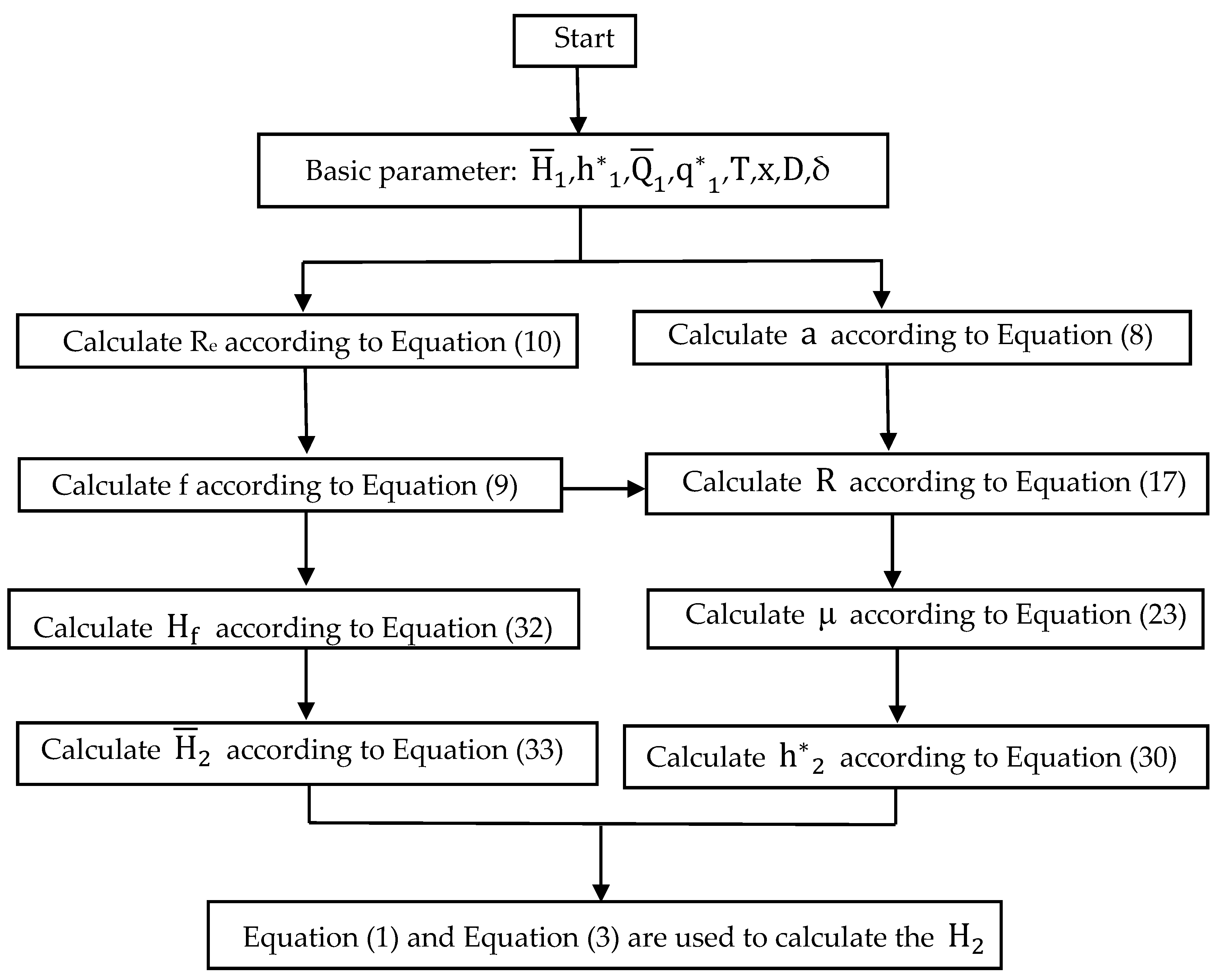
Figure 4 shows a flowchart for calculating the instantaneous pressure head of oscillating water flow.

3. Results and Discussion

3.1. Results

Using the calculation model (Section 2.2),

Table 2. The measured and calculated values of the amplitude of the pressure head along the pipeline.

Pipe Length (m)		D1			D2			D3
	Calculated Value (m)	Measured Value (m)	Relative Error (%)	Calculated Value (m)	Measured Value (m)	Relative Error (%)	Calculated Value (m)	Measured Value (m)	Relative Error (%)
0	8.00	7.91	1.14	6.00	6.10	1.64	2.00	2.05	2.44
12	7.54	7.88	4.31	5.63	5.46	3.11	1.88	1.94	3.09
24	7.07	6.69	5.68	5.27	5.69	7.38	1.76	1.88	6.38
36	6.61	6.04	9.44	4.90	5.05	2.97	1.64	1.56	5.13
48	6.15	6.53	5.82	4.54	4.17	8.87	1.52	1.67	8.98
60	5.69	5.32	6.95	4.18	3.93	6.36	1.41	1.53	7.84

shows the measured and calculated value of the amplitude of the pressure head along the pipeline for Case D1, D2, and D3.

Table 3. The measured and calculated values of the average instantaneous pressure head along the pipeline.

Pipe Length (m)		D1			D2			D3
	Calculated Value (m)	Measured Value (m)	Relative Error (%)	Calculated Value (m)	Measured Value (m)	Relative Error (%)	Calculated Value (m)	Measured Value (m)	Relative Error (%)
0	16.00	15.91	0.57	10.00	9.94	0.60	8.00	7.92	1.01
12	15.15	15.32	1.11	9.48	9.83	3.56	7.54	7.26	3.86
24	14.30	14.76	3.12	8.95	9.18	2.51	7.08	7.28	2.75
36	13.45	12.79	5.16	8.43	8.02	5.11	6.62	6.14	7.82
48	12.60	13.65	7.69	7.90	8.52	7.28	6.16	6.61	6.81
60	11.74	12.54	6.38	7.38	6.81	8.37	5.70	5.30	7.55

shows the measured and calculated value of the average instantaneous pressure head along the pipeline for Case D1, D2, and D3. In Case D1, D2, and D3, the maximum relative error ($\frac{\left|\mathrm{Measured}\mathrm{value}-\mathrm{Calculated}\mathrm{value}\right|}{\mathrm{Measured}\mathrm{value}}\times 100\%$) of the calculated and measured value of the amplitude of the pressure head along the pipeline was 9.44%. The maximum relative error of the calculated and measured value of average instantaneous pressure head along the pipeline was 8.37%. These results show that the amplitude of the pressure head and the average instantaneous pressure head calculated by the calculation model are accurate. Therefore, the model can be used to calculate the instantaneous pressure heads of oscillating water flow in a pipeline.

Figure 5 shows the measured and calculated values of the instantaneous pressure head at 12 and 60 m pipe lengths for Case D1, D2, and D3. It can be seen that the calculated and measured instantaneous pressure heads are close to each other. It can also be seen from Figure 5 that the period remains unchanged when oscillating water flows along the pipeline.

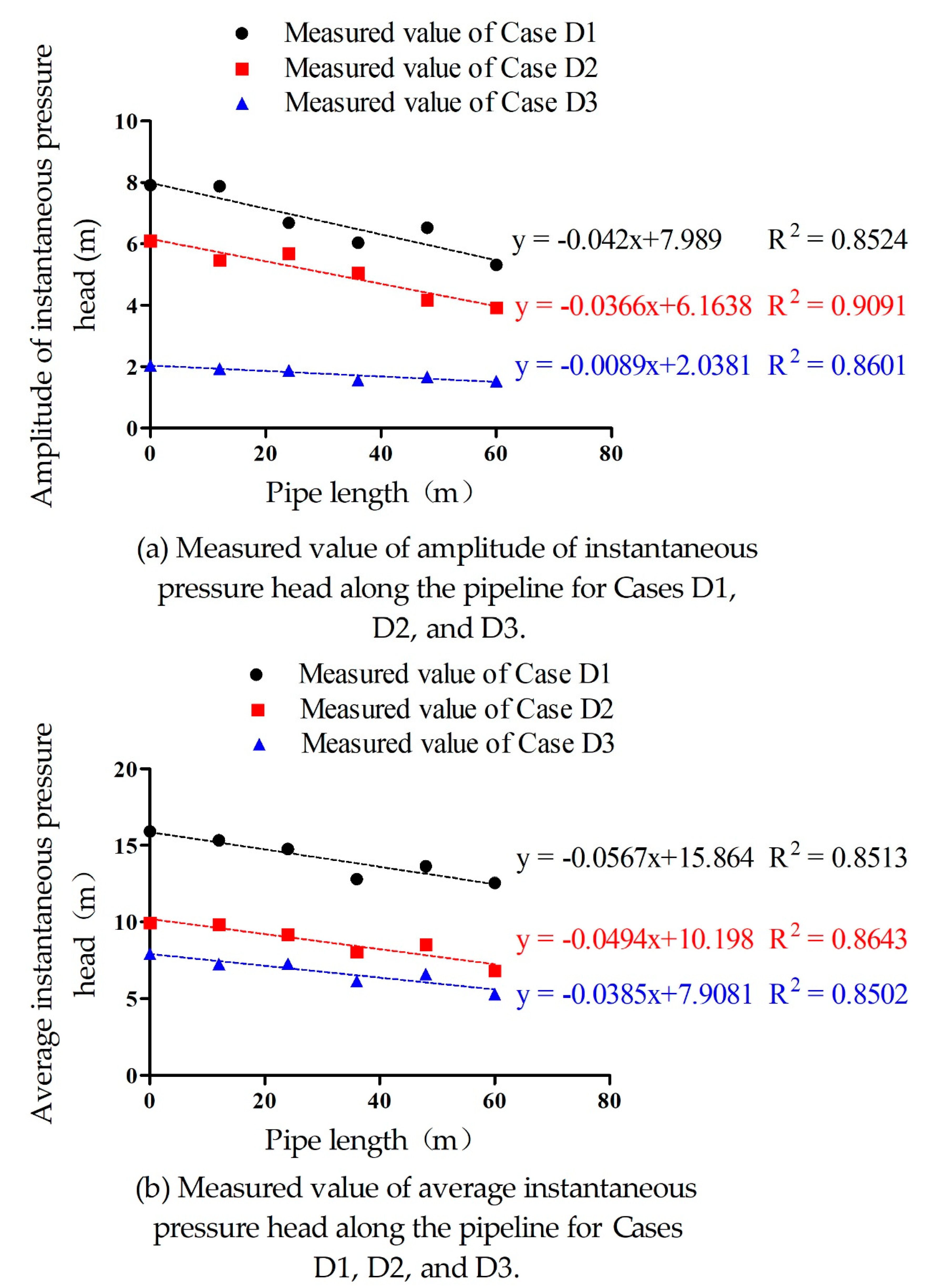
Figure 6 shows the measured value of the amplitude of the pressure head and the average instantaneous pressure head along the pipeline for Case D1, D2, and D3. It can be seen that the amplitude of the pressure head and the average instantaneous pressure head decrease linearly along the pipeline. The instantaneous pressure head loss of oscillating water flow in the pipeline is caused by the friction resistance of the pipeline to the flow and the drastic change of discharge, which leads to the powerful mixing and collision of water particles. The relevant laws can provide a basis for further research in the calculation of the instantaneous pressure head of oscillating water flow.

3.2. Discussion

In this study, the calculation model for the instantaneous pressure head of oscillating water flow along a pipeline was developed. In order to verify the accuracy of the calculation results from the model, three cases (Cases D1, D2, and D3) were tested. The experimental results show that the model can be used to accurately calculate the instantaneous pressure head of oscillating water flow along the pipeline. However, using the model developed in this study to calculate the amplitude of the pressure head of oscillating water flow requires a lot of complicated calculations to be solved by a computer. To some extent, it is less convenient and inefficient to calculate the amplitude of the pressure head of oscillating water flow using the model in the practical design of irrigation pipeline network, especially without the help of computer. Therefore, it is necessary to develop formulas that are more convenient and efficient to calculate the amplitude of the pressure head of oscillating water flow. The development of the model in this study can be used as a theoretical basis for developing formulas, for example, the influencing factors affecting the movement of oscillating water flow in a pipeline in the model. These influencing factors include the flow influencing factors (e.g., amplitude of pressure head, amplitude of discharge, period, equivalent bulk modulus of water, density of water, kinematic viscosity of water) and the pipeline influencing factors (e.g., inner radius of the pipe, thickness of the pipe wall, modulus of elasticity of the pipe material). The amplitude of the pressure head and the average instantaneous pressure head both decrease linearly along the pipeline. These theoretical bases can be used to further simplify and optimize the model and to develop the formula. Further, they are of great significance for the design of irrigation pipe networks and the wide application of oscillating water flow in irrigation systems.

4. Conclusions

By using a complex function to solve the continuity equation and the momentum equation of a pipeline with water hammer motion and using the Darcy–Weisbach formula to estimate the head loss, a calculation model for the instantaneous pressure head of oscillating water flow along a pipeline was developed. The measured values of the amplitude of the pressure head and the average instantaneous pressure head in the experiments were used to verify the corresponding pressure head calculated by the model. The results show that the amplitude of the pressure head and the average instantaneous pressure head decrease linearly along the pipeline. The calculated value of the amplitude of the pressure head and the average instantaneous pressure head are basically close to the corresponding measured pressure heads. From the results of all the tests, the maximum relative error of the calculated and measured value of amplitude of pressure head along the pipeline was 9.44%. The maximum relative error of the calculated and measured value of average instantaneous pressure head along the pipeline was 8.37%. Hence, the model can accurately predict the instantaneous pressure head of oscillating water flow along a pipe and provide a theoretical basis for the application of oscillating water flow in irrigation systems and the design of irrigation pipe networks.

References

- Woltering, L.; Ibrahim, A.; Pasternak, D.; Ndjeunga, J. The economics of low pressure drip irrigation and hand watering for vegetable production in the Sahel. Agric. Water Manag. 2011, 99, 67–73. [Google Scholar] [CrossRef] [Green Version]
- Marsh, B.; Dowgert, M.; Hutmacher, R.; Phene, C.J. Low-pressure drip system in reduced tillage cotton. WIT Ecol. Environ. 2007, 103, 73–80. [Google Scholar]
- Kranz, W.L.; Eisenhauer, D.E.; Retka, M.T. Water and energy-conservation using irrigation scheduling with center-pivot irrigation systems. Agric. Water Manag. 1992, 22, 325–334. [Google Scholar] [CrossRef]
- O’Shaughnessy, S.A.; Evett, S.R.; Andrade, M.A.; Workneh, F.; Price, J.A.; Rush, C.M. Site-specific variable-rate irrigation as a means to enhance water use efficiency. Trans. ASABE 2016, 59, 239–249. [Google Scholar]
- Singh, A.K.; Sharma, S.P.; Upadhyaya, A.; Rahman, A.; Sikka, A.K. Performance of low energy water application device. Water Resour. Manag. 2010, 24, 1353–1362. [Google Scholar] [CrossRef]
- Wei, Q.S.; Lu, G.; Liu, J.; Shi, Y.S.; Dong, W.C.; Huang, S.H. Evaluations of emitter clogging in drip irrigation by two-phase flow simulations and laboratory experiments. Comput. Electron. Agric. 2008, 63, 294–303. [Google Scholar]
- Oron, G.; Demalach, J.; Hoffman, Z.; Cibotaru, R. Subsurface microirrigation with effluent. J. Irrig. Drain. Eng. ASCE 1991, 117, 25–36. [Google Scholar] [CrossRef]
- Zhai, G.L.; Lv, M.C.; Wang, H.; Xiang, H.A. Plugging of microirrigation system and its prevention. Trans. Chin. Soc. Agric. Eng. 1999, 15, 144–147. [Google Scholar]
- Shamshery, P.; Winter, A.G. Shape and form optimization of on-line pressure-compensating drip emitters to achieve lower activation pressure. J. Mech. Design 2018, 140, 035001. [Google Scholar] [CrossRef]
- Sayyadi, H.; Nazemi, A.H.; Sadraddini, A.A.; Delirhasannia, R. Characterising droplets and precipitation profiles of a fixed spray-plate sprinkler. Biosyst. Eng. 2014, 119, 13–24. [Google Scholar] [CrossRef]
- Seginer, I.; Kantz, D.; Nir, D. The distortion by wind of the distribution patterns of single sprinklers. Agric. Water Manag. 1991, 19, 341–359. [Google Scholar] [CrossRef]
- Li, G.Y.; Wang, J.D.; Alam, M.; Zhao, G.Y. Influence of geometrical parameters of labyrinth flow path of drip emitters on hydraulic and anti-clogging performance. Trans. ASABE 2006, 49, 637–643. [Google Scholar] [CrossRef]
- Yu, L.M.; Li, N.; Liu, X.G.; Yang, Q.L.; Li, Z.Y.; Long, J. Influence of dentation angle of labyrinth channel of drip emitters on hydraulic and anti-clogging performance. Irrig. Drain. 2019, 68, 256–267. [Google Scholar] [CrossRef]
- Zhang, J.; Zhao, W.H.; Tang, Y.P.; Lu, B.H. Anti-clogging performance evaluation and parameterized design of emitters with labyrinth channels. Comput. Electron. Agric. 2010, 74, 59–65. [Google Scholar] [CrossRef]
- Zhang, J.; Zhao, W.H.; Tang, Y.P.; Lu, B.H. Structural optimization of labyrinth-channel emitters based on hydraulic and anti-clogging performances. Irrig. Sci. 2011, 29, 351–357. [Google Scholar] [CrossRef]
- Liu, J.; Yuan, S.; Li, H.; Zhu, X. Combination uniformity improvement of impact sprinkler. Trans. Chin. Soc. Agric. Eng. 2011, 27, 107–111. [Google Scholar]
- Li, H.; Jiang, Y.; Xu, M.; Li, Y.; Chen, C. Effect on hydraulic performance of low-pressure sprinkler by an intermittent water dispersion device. Trans. ASABE 2016, 59, 521–532. [Google Scholar]
- Yuan, S.; Wei, Y.; Li, H.; Xiang, Q. Structure design and experiments on the water distribution of the variable-rate sprinkler with non-circle nozzle. Trans. Chin. Soc. Agric. Eng. 2010, 26, 149–153. [Google Scholar]
- Zhang, L.; Wu, P.; Zhu, D.; Zheng, C. Effect of oscillating pressure on labyrinth emitter clogging. Irrig. Sci. 2017, 35, 267–274. [Google Scholar] [CrossRef]
- Zheng, C.; Wu, P.T.; Zhang, L.; Zhu, D.L.; Zhao, X.; An, B.D. Particles movement characteristics in labyrinth channel under different dynamic water pressure modes. Trans. Chin. Soc. Agric. Mac. 2017, 48, 294–301. [Google Scholar]
- Yu, L.M.; Li, N.; Liu, X.G.; Yang, Q.L.; Long, J. Influence of flushing pressure, flushing frequency and flushing time on the service life of a labyrinth-channel emitter. Biosyst. Eng. 2018, 172, 154–164. [Google Scholar] [CrossRef]
- Zhang, K.; Song, B.; Zhu, D. The influence of sinusoidal oscillating water flow on sprinkler and impact kinetic energy Intensities of laterally-moving sprinkler irrigation systems. Water 2019, 11, 1325. [Google Scholar] [CrossRef]
- Hills, D.J.; Silveira, R.C.M.; Wallender, W.W. Oscillating pressure for improving application uniformity of spray emitters. Trans. ASABE 1986, 29, 1080–1085. [Google Scholar] [CrossRef]
- Hills, D.J.; Gu, Y.P.; Wallender, W.W. Sprinkler uniformity for oscillating low water-pressure. Trans. ASABE 1987, 30, 729–734. [Google Scholar] [CrossRef]
- Buchin, A.J.; Pons, S.J.; Hills, D.; Abudu, S. Improving Water Application Efficiency in the Landscape through Pressure Oscillation. April 2004. Available online: https://www.researchgate.net/publication/237342500 (accessed on 1 April 2019).
- Tijsseling, A.S. Water hammer with fluid–structure interaction in thick-walled pipes. Comput. Struct. 2007, 85, 844–851. [Google Scholar] [CrossRef]
- Ghidaoui, M.S.; Mansour, S.G.S.; Zhao, M. Applicability of quasisteady and axisymmetric turbulence models in water hammer. J. Hydraul. Eng. 2002, 128, 917–924. [Google Scholar] [CrossRef]
- Zhang, B.; Wan, W.; Shi, M. Experimental and numerical simulation of water hammer in gravitational pipe flow with continuous air entrainment. Water 2018, 10, 928. [Google Scholar] [CrossRef]
- Kochupillai, J.; Ganesan, N.; Padmanabhan, C. A new finite element formulation based on the velocity of flow for water hammer problems. Int. J. Pres. Ves. Pip. 2005, 82, 1–14. [Google Scholar] [CrossRef]
- Besharat, M.; Teresa, V.M.; Ramos, H. Experimental study of air vessel behavior for energy storage or system protection in water hammer events. Water 2017, 9, 63. [Google Scholar] [CrossRef]
- Zheng, C.; Wu, P.T.; Zhang, L.; Zhu, D.L.; Chen, X.; Chen, J.Y. Flow characteristics in labyrinth channel under dynamic water pressure. Trans. Chin. Soc. Agric. Mac. 2015, 46, 167–172. [Google Scholar]
- Wylie, E.B.; Streeter, V.L.; Suo, L. Fluid Transients in Systems; Prentice Hall, Inc.: Englewood Cliffs, NJ, USA, 1993. [Google Scholar]
- Halliwell, A.R. Velocity of a water-hammer wave in an elastic pipe. J. Hydraul. Div. 1963, 89, 1–21. [Google Scholar]
- Young, W.C.; Budynas, R.G.; Sadegh, A.M. Roark’s Formulas for Stress and Strain; McGraw-Hill, Inc.: New York, NY, USA, 2002. [Google Scholar]
- Mäkinen, J.; Piche, R.; Ellman, A. Fluid transmission line modeling using a variational method. J. Dyn. Syst. Meas. ASME 2000, 122, 153–162. [Google Scholar] [CrossRef]
- Capponi, C.; Zecchin, A.C.; Ferrante, M.; Gong, J.Z. Numerical study on accuracy of frequency-domain modelling of transients. J. Hydraul. Res. 2017, 55, 813–828. [Google Scholar] [CrossRef]
- Chaudhry, H.M. Applied Hydraulic Transients; Van Nostrand Reinhold, Inc.: New York, NY, USA, 1979. [Google Scholar]
- Allen, R.G. Relating the Hazen-Williams and Darcy-Weisbach friction loss equations for pressurized irrigation. Appl. Eng. Agric. 1996, 12, 685–694. [Google Scholar] [CrossRef]
Figure 1.
Schematic diagram of oscillating water pressure.
Figure 2.
Test platform for measuring instantaneous pressure head of oscillating water flow. PLC—programmable logic controller.
Figure 3.
Locations of cross-section 1–1 and cross-section 2–2 along the pipeline.
Figure 4.
Flowchart for calculating the instantaneous pressure head of oscillating water flow.
Figure 5.
The measured and calculated value of instantaneous pressure head at 12 and 60 m pipe lengths for (a) Case D1, (b) Case D2, and (c) Case D3.
Figure 6.
The measured value of (a) amplitude of pressure head and (b) average instantaneous pressure head along the pipeline for Cases D1, D2, and D3.