Assessment of System Responses in Intensively Irrigated Stream–Aquifer Systems Using SWAT-MODFLOW

Department of Civil and Environmental Engineering, Colorado State University, 1372 Campus Delivery, Fort Collins, CO 80523-1372, USA
*
Author to whom correspondence should be addressed.
Water 2019, 11(8), 1576; https://doi.org/10.3390/w11081576
Submission received: 26 June 2019
/
Revised: 12 July 2019
/
Accepted: 22 July 2019
/
Published: 30 July 2019
(This article belongs to the Section Hydrology)
Abstract
:Water management strategies need to balance water security and food production, particularly in semi-arid regions wherein irrigation is required to supplement rainfall. Irrigated stream–aquifer systems present a unique challenge in this effort, due to complex groundwater–surface water interactions and the high level of human intervention in managing irrigation practices. This paper has two objectives: first, to detail a method for constructing and applying a coupled SWAT-MODFLOW to irrigated stream–aquifer systems; and second, to use the model to quantify the effects of decreasing irrigation on hydrological responses and crop yield. The method is applied to a 734 km2 study region in the Lower Arkansas River Valley, an alluvial valley in Colorado, USA, which has been intensively irrigated for over 100 years and is threatened by shallow water tables. Therefore, a reduction in applied irrigation amounts has the double benefit of conserving water and decreasing waterlogging, given that crop yield can be maintained for food production. The results indicate that an approximate 10% decrease in total applied irrigation water results in decreases of 6% in surface runoff, 8% in evapotranspiration, and 4% in recharge water. It also results in an increase of 4% in groundwater return flow to the Arkansas River, and an actual increase in groundwater levels due to the decrease in groundwater pumping, pointing to the need for targeted irrigation reduction strategies to decrease waterlogging occurrence. The irrigation reduction yields an average 9% decrease in corn and alfalfa yield. This modeling approach is in general transferable to other similar irrigated river valleys.
1. Introduction
The increasing scarcity of water is an immediate threat to the sustainable development of areas around the world. Water resource managers faces the growing challenges of providing sustainable water supplies while maintaining and even increasing crop productivity, all in the face of increasing demand, limited resources, and the variation of streamflow and groundwater volumes due to short-term human management and long-term climatic patterns [1,2,3,4]. The optimum management of available groundwater and surface water resources is particularly difficult in irrigated stream–aquifer systems due to the interaction between groundwater and surface water and the high degree of human intervention in providing irrigation water to cultivated fields. Both groundwater and surface water are used for irrigation, with recharge to the alluvial aquifer providing return flow to streams [5,6,7,8,9]. However, in many regions, high water tables result in waterlogging, soil salinization, and nutrient accumulation in the aquifer and downstream areas [10,11,12,13,14,15]. Therefore, water management strategies in these regions must balance water conservation with crop yield while also seeking to lower groundwater levels.
Due to the complexity in these systems, watershed-scale hydrological models have been essential tools to capture the major hydrological processes and investigate solutions through alternative management strategies [16,17,18,19]. Some of the commonly used models focus on land surface processes, and include the Agricultural NonPoint Source pollution model (AGNPS [20]), the Hydrological Simulation Program—Fortran (HSPF [21]), the Hydrologic Modeling System (HEC-HMS; [22]), the KINematic runoff and EROSion model (KINEROS [23]), the Soil and Water Assessment Tool (SWAT [24]), the Soil and Water Integrated Model (SWIM [25]), and the CASCade of planes in 2-Dimentions (CASC2D [26]).
SWAT, the most popular of these, is considered a promising tool for continuous simulations in predominantly agricultural watersheds, and often is used to assess changes in water due to land use and agricultural management practices [27,28,29,30,31]. For example, SWAT was used to evaluate impacts of various dairy farming facts on land-use changes in the 3050 km2 Sondu River basin in Kenya [32], and to analyze the implementation of land management practices to improve water quantity and maintain crop production in Central German [33]. In the Midwest United States, a study used the SWAT model to explore the response of crop yield to climate variability and estimate crop yield under different drought and aeration stresses conditions [34]. SWAT also has been applied in the Aral Sea drainage basin in northwest Iran to access water savings as a result of improved irrigation techniques [35]. This study showed that changing the traditional irrigation system to a pressurized irrigation system can lead to basin level water conservation and increase crop production. However, they did not capture the individual hydrological responses, especially the interactions of groundwater and surface water [36]. The current SWAT model often performs poorly in watershed systems wherein groundwater discharge is a significant component of streamflow [27,37,38], due to lack of consideration of geographic location of groundwater and spatially-varying aquifer characteristics. In addition, the influence of pumping wells on groundwater head gradients cannot be simulated.
Spatio-temporal hydrological processes and water management assessment can also be addressed through integrated models such as CATchment HYdrology (CATHY [39]), the Ground-water and Surface-water Flow Model (GSFLOW [40]); Parallel groundwater Flow (ParFLOW [41]), HydroGeoSphere [42], OpenGeoSys (OGS [43]), and MIKE SHE [44]. Examples of applying these integrated models for investigating management strategies include the application of GSFLOW to the second largest inland river basin in China [45] to perform temporal optimization for the conjunctive use of surface water and groundwater for irrigation, and applying MIKE SHE to analyze the influence of groundwater dynamics in the estimation of hydrology–land surface feedback in a 225 km2 region in Kansas [46]. While many studies focus on assessing groundwater surface–water interactions under climate change [47,48], agronomic and environmental feedbacks [6,49,50,51], and wetland interactions [52,53], there is a need for an assessment of land management practices on hydrological processes and agronomic responses in a fully integrated stream–aquifer systems wherein major human interventions in managing irrigation practices occur.
The objective of this study is twofold: first, to detail a method for constructing and applying a coupled SWAT-MODFLOW (modular three-dimensional finite-difference groundwater model - MODFLOW) to irrigated stream–aquifer systems; and second, to use the model to quantify the effects of decreasing irrigation on hydrologic responses and food production (i.e., crop yield). System responses include stream flow, groundwater elevation, groundwater discharge to streams, and crop yield. The objective will be accomplished through the use of a coupled groundwater surface SWAT-MODFLOW model that links SWAT with MODFLOW [54], which is a widely used groundwater flow model. Whereas previous model applications to this study region focused on groundwater flow [55] (MODFLOW using the River package) and groundwater flow with streamflow [50] (MODFLOW using the Streamflow Routing package), the use of SWAT-MODFLOW provides a representation of all major hydrologic processes, including surface runoff and soil lateral flow. In addition, the inclusion of SWAT allows for the simulation of crop yield. Although the model is based on the published SWAT-MODFLOW modeling code [56], it has been modified to include detailed representations of canal diversion, canal seepage, applied irrigation amounts of surface water (canals), and groundwater (pumping wells) for each field, and the evapotranspiration of shallow groundwater. The model is applied to a 732 km2 region of the Lower Arkansas River Valley (LARV) in southeastern Colorado, an intensively irrigated system in which shallow water tables have caused waterlogging and associated soil salinization in recent decades. The model is calibrated and tested against land surface and subsurface system-response variables as well as crop yield.
Section 2 provides a brief theoretical overview of SWAT, MODFLOW, and the coupled SWAT-MODFLOW model, followed by modifications of the SWAT-MODFLOW code to enhance model capability in irrigated stream–aquifer systems. Section 3 demonstrates the method of applying the modified SWAT-MODFLOW code to the LARV, and Section 4 provides results and a discussion.
2. Model Construction and Composition
2.1. Overview of SWAT and MODFLOW
The Soil and Water Assessment Tool (SWAT) is a continuous time, physically-based, and spatially semi-distributed model [24]. It has been successfully used to test and evaluate eco-hydrological processes containing surface and soil water flow, nutrient mass transport, food production, and land-use management practices at the watershed scale [57,58,59,60,61,62]. The watershed is typically divided into multiple sub-basins based on topography. Hydrologic response units (HRUs) in each sub-basin are created by lumping similar land-use and soil layers in which the vertical flows and nutrient transport are calculated. The output from each HRU is routed according to the channel routing algorithm to the watershed outlet. A main disadvantage of SWAT is its lumped, linear reservoir approach, which oversimplifies the groundwater processes. It results in significant conceptual limitations regarding the physical representation of the aquifer heterogeneity, groundwater flow, and the surface and subsurface interactions in the hydrological system.
The modular three-dimensional finite-difference groundwater model (MODFLOW) is a physically based, fully distributed model [54]. It uses the finite different approach to solve the groundwater flow equations for the hydraulic head in each grid cell based on sources and sinks (e.g., recharge, pumping), initial and boundary conditions, and aquifer parameters (e.g., river conductance, specific storage, specific yield, and hydraulic conductivity). MODFLOW has various packages that simulate different hydrological processes, such as soil deep percolation (i.e., water that leaves the bottom of the soil profile) is considered by recharge package (RCH), groundwater pumping/injection is represented by well package (WEL), groundwater discharge/recharge is simulated by the river package (RIV) along the river grid cells, and the evapotranspiration package (EVT) evaluates groundwater upflux to evapotranspiration when the groundwater table raises into the root zone. A recent version is MODFLOW-NWT, which performs well in unconfined groundwater systems with the complex non-linear drying and rewetting processes [63]. MODFLOW lacks a meaning of specifying the conditions in terms of hydrological processes at the watershed surface. Therefore, it is often linked with land surface models such as SWAT [56,64,65,66], as is done in the study we addressed in this paper.
2.2. SWAT-MODFLOW Linkage
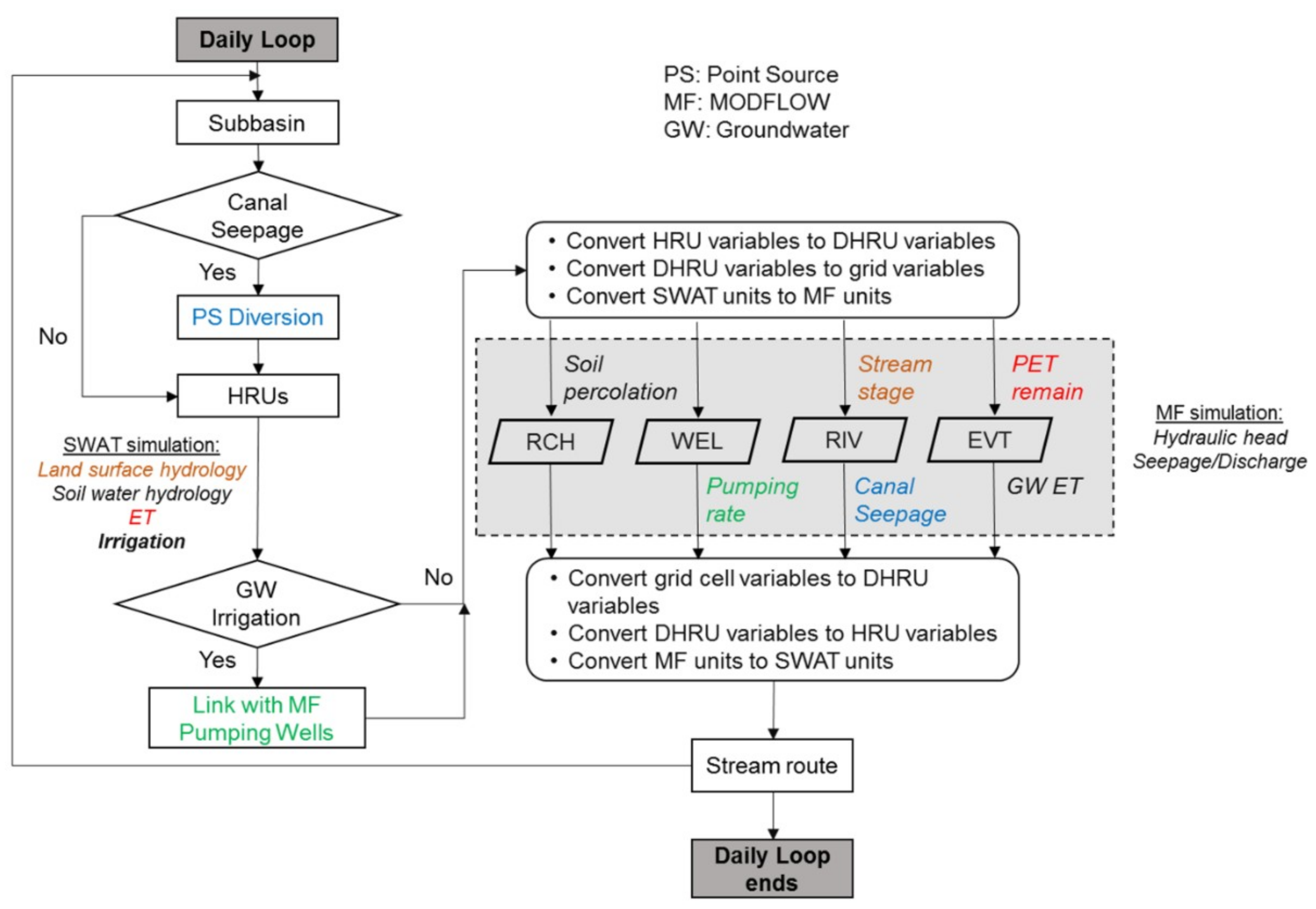
The SWAT-MODFLOW modeling code [56] combines the SWAT 2012 and MODFLOW-NWT, a Newton-Raphson formulation for MODFLOW-2005, into a single FORTRAN code, which replaces the SWAT groundwater module with the MODFLOW code. The fundamental linkage between the two models is based on mapping schemes that occur on a daily time step that passes SWAT-calculated deep percolation as a recharge to the MODFLOW grid cell. Then, the MODFLOW-calculated hydraulic head is compared with the SWAT stream channels to determine stream–aquifer interactions on a daily time step. The SWAT HRUs are first split into disaggregated HRUs (DHRUs), in which each DHRU contains a geographical location to store SWAT daily calculations (e.g., soil deep percolation). All the mapping information is stored in four text inputs files that are read at the beginning of the simulation. Within the framework, SWAT simulates surface and soil zone processes (e.g., stream stage, surface runoff, overland flow, lateral flow, surface evapotranspiration, and plant growth), while MODFLOW simulates groundwater hydrology in each grid cell (e.g., groundwater elevation, three-dimensional groundwater flow, and surface–groundwater interactions). The main steps in the daily loop of the SWAT-MODFLOW code are shown in Figure 1.
2.3. SWAT-MODFLOW Modifications
Modifications to the SWAT-MODFLOW code are made for simulating irrigation-related processes in the irrigated stream–aquifer system. These include new subroutines for groundwater irrigation and groundwater evapotranspiration, as detailed in the following sections.
2.3.1. Irrigation Events
The SWAT automatic irrigation algorithm is applied to represent irrigation events that can be triggered based on plant water demand [67]. Irrigation water can be provided either by surface water through earthen canals or by groundwater through pumping wells. For surface water irrigation, the standard SWAT procedure is used by specifying the sub-basin reach from which the surface water is derived, representing canal diversions from the main stem of the river. For groundwater irrigation, as can be seen in Figure 1, daily pumping rates are specified in the MODFLOW’s WEL package input file, with these volumes converted to irrigation depths for application to SWAT HRUs on the following day. The conversion of volumes to depths and the application to SWAT HRUs are performed using new subroutines within the SWAT-MODFLOW code. To employ this new model linkage, the model user must prepare a file (swatmf_irrigate.txt) that contains the following information:
- HRUs and associated sub-basin assigned to each pumping well, with the pumping well designated by a row and column within the MODFLOW grid;
- Conveyance efficiency for each subbasin (percentage of pumped groundwater that is lost between the well and the field of application, representing loss from an earthen canal); and
- Runoff ratio (percentage of applied irrigation water that runs off the field).
The depth of irrigation water to the groundwater-supplied HRU via a pumping well is calculated as:
where Vsub-irr,i is the total volume of irrigation water provided to SWAT sub-basin i (m3/day); Qpump,n,i is the amount of water pumped for a specified grid cell n for a given sub-basin i (m3/day); Rconvey,i is conveyance efficiency for a given sub-basin i; Dsub-irr,i is the depth of irrigation provided to SWAT sub-basin i (mm), with the 1000 included to convert from meters to mm; Ai is the total HRU area that receives irrigation water in a given sub-basin i; airdj is the amount of irrigation water applied to a given HRU j; and Rrunoff,i is the runoff efficiency for a given sub-basin i. The irrigation depths for the groundwater-supplied HRUs are applied on the following day.
2.3.2. Groundwater Evapotranspiration
Due to the presence of shallow water tables in many semi-arid irrigated regions, the volume of groundwater removed via evapotranspiration (ET) is calculated as a linearly varying function of depth below the water table using MODFLOW’s EVT package. The EVT package simulates the influence of direct evaporation and plant transpiration in removing water from the saturated groundwater regime based on the following assumptions: (1) when the groundwater elevation is at or above the root zone, which is the bottom layer of SWAT soil profile, ET from the water table occurs with a user specified maximum rate; (2) when the groundwater elevation is below a specified extinction depth, ET from the saturated zone ceases; (3) between these two limits, ET from the water table varies linearly with groundwater elevation [68]. The maximum evapotranspiration rate EVTR provided to the EVT package is calculated as the difference between the potential ET rate (PET) (mm) calculated by SWAT and the actual ET rate (AET) (mm) simulated by SWAT:
with the assumption that a portion of the PET rate can be satisfied by the shallow water table.
Therefore, this coupling process is effective in the new coupling code when the groundwater table is within the root zone. With other SWAT-MODFLOW interactions, groundwater ET is simulated on a daily time step.
3. SWAT-MODFLOW Application to Irrigated Stream–Aquifer System
3.1. Study Region: Lower Arkansas River Valley, Colorado
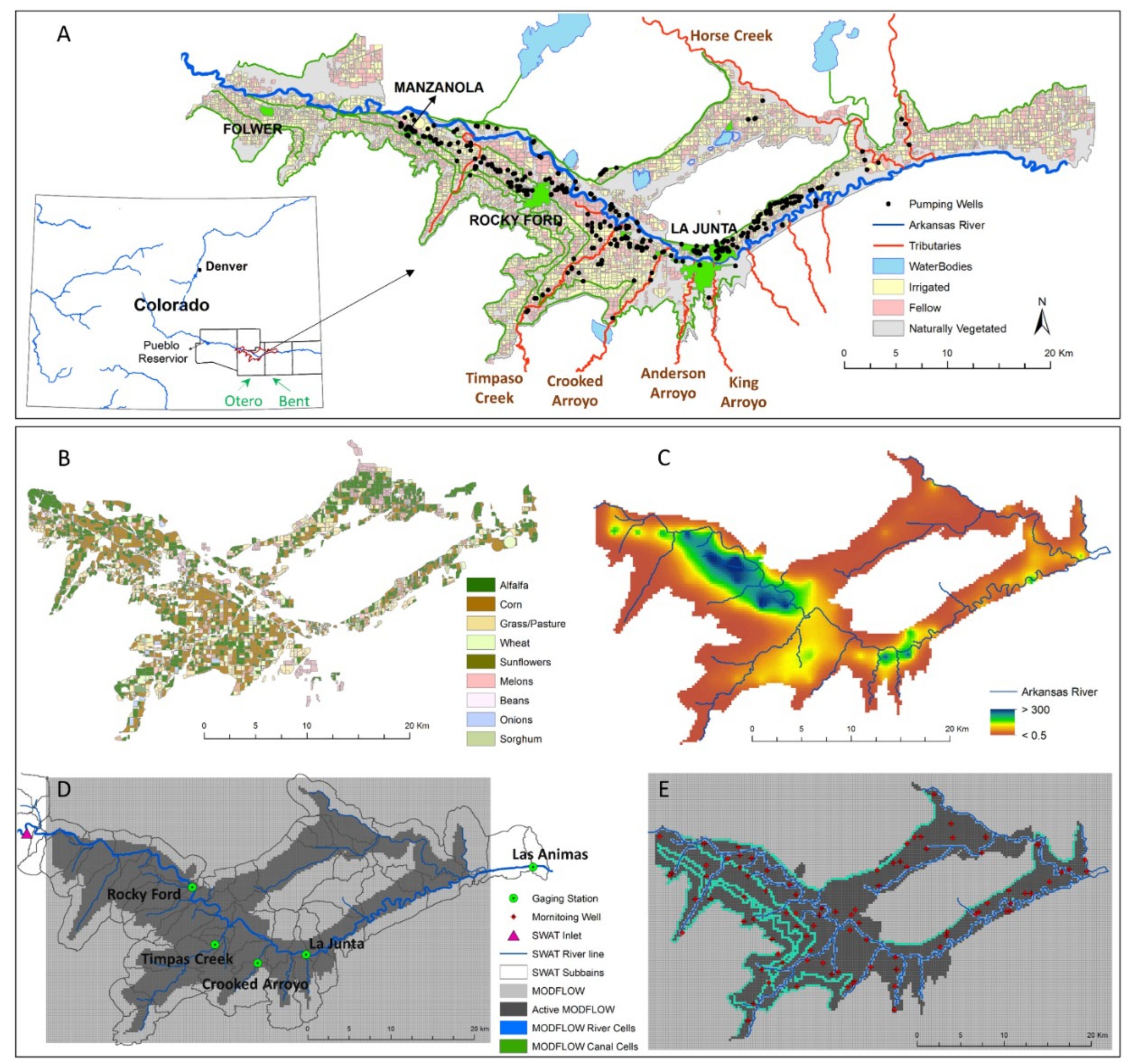
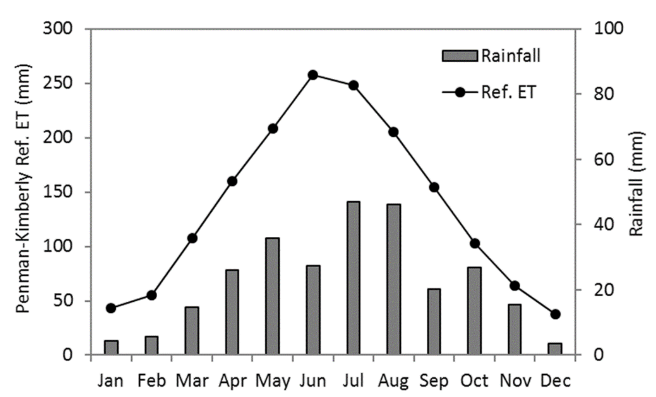
The modified SWAT-MODFLOW code is illustrated in application to a 732 km2 irrigated stream–aquifer system along the Lower Arkansas River Valley (LARV) in southeastern Colorado (Figure 2A). In this study region, the snowmelt-derived Arkansas River runs through a shallow sandy alluvial aquifer (10–20 m in thickness) that contains two main tributaries, Timpas Creek and Crooked Arroyo. The average temperature is 13.6 °C, with the monthly temperature varies between −7/9 °C (low/high) and 16/33 °C in December and July, respectively. The mean annual crop reference evapotranspiration (ETr; Alfalfa reference equation) is about 1650 mm, which is much larger than the mean annual precipitation of 273 mm (Figure 3). Two-thirds of the annual rainfall occurs between April and August, primarily during brief but intense thunderstorms.
The climate is semi-arid, which requires irrigation to supplement rainfall for crop growth. Over the past century, irrigation has been practiced either through diverting water from the Arkansas River into an extensive network of earthen canals (Figure 2A green lines), or more recently from the aquifer through a network of 575 pumping wells (Figure 2A black dots). From 89 groundwater observation wells (Figure 2E red dots), the groundwater table is 2–20 m below the surface. Groundwater recharge is provided by the infiltration of precipitation, percolation of applied irrigation, and seepage from river, canals, and ditches [69], with the increased groundwater head creating a gradient that produces discharge to the stream network, creating baseflow for the river. Cultivation and associated irrigation occurred between March–November. Figure 2B shows the crop type information for each cultivated field in 1999, provided by information from the Farm Service Agency located in Rocky Ford, Colorado. Alfalfa, corn, and wheat are the dominant crop types in the LARV.
3.2. Model Application
The SWAT-MODFLOW model for the study region uses the calibrated SWAT model [67] and the calibrated MODFLOW model [55], with the latter developed to study the impacts of human management features on hydrological processes in an irrigated watershed.
The SWAT model used for the study area was developed by a former study [67]. The region includes 72 sub-basins (Figure 2D). As described in the previous paper [67], a method was developed to apply SWAT to intensively managed irrigated watershed, which included: (1) designating each cultivated field as an HRU; (2) manipulating realistic crop rotations by changing the management files (*.mgt) for each HRU; and (3) applying SWAT’s automatic irrigation function to trigger irrigation events based on plant water demand for both surface water and groundwater irrigation. This method required modifications to the input files and resulted in 5270 HRUs. The source of surface irrigation water for all HRUs in a given canal command area was specified to the section of the Arkansas River coinciding with the point of diversion based on the Colorado Division of Water Resources. Groundwater irrigation was specified to HRUs surrounded by the groundwater pumps. Additional details on model construction have been provided by the original SWAT study [67]. The model was run from April 1999 to Feburary 2016, with simulated streamflow tested against observed hydrographs at five stream gauges (See Figure 2D for location) [67].
The original MODFLOW model encompasses the central cultivated region with an area of 506 km2. The region was discretized into finite difference grid cells with uniform dimensions of 250 m × 250 m, consisting of 213 east–west oriented rows and 127 north–south oriented columns (see Figure 2D in light grey) with 7777 activated cells (see Figure 2D in dark grey) in the model domain. The model consists of 1943 river cells, of which 1089 represent the Arkansas River and tributaries (Figure 2E in blue), and 1065 represent irrigation canals (Figure 2E in green). The aquifer was discretized vertically into two layers of varying thickness based on the local hydrogeological units, with a third layer representing the shale bedrock. The MODFLOW WEL package simulated groundwater pumping processes, while the unsaturated-zone processes were represented using the UZF1 package, including weekly infiltrated irrigation and precipitation depths, potential evapotranspiration, and unsaturated zone flow for each grid cell. Surface water and groundwater interactions were estimated using the RIV package. The model was tested against water table elevation, groundwater return flow to the river network, and ET.
The spatial extent of the coupled SWAT-MODFLOW model is shown in Figure 2D. The SWAT-MODFLOW linkage has the ability to use SWAT and MODFLOW models of different spatial extent. The original functionality of each model is retained beyond the overlap area. The modification to the original MODFLOW was the replacement of the UZF1 package by the EVT and RCH packages. As described in Section 2.3.2, groundwater ET processes are simulated using the EVT package. Daily diverted volumes from the Arkansas River to irrigation canals are simulated as point sources along SWAT stream channels.
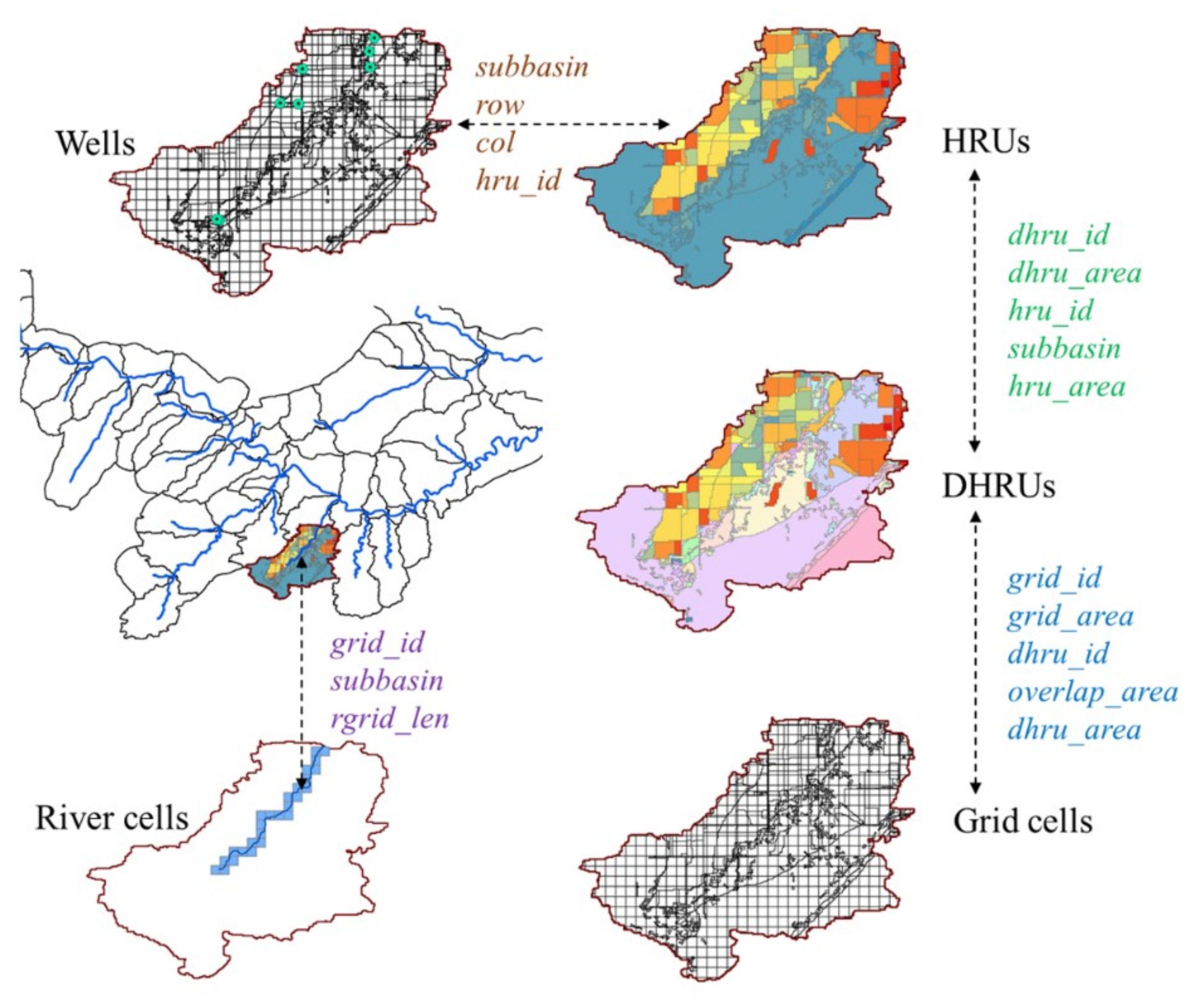
The basic procedure of linking two models is processed using ArcGIS. Both DHRUs and SWAT stream networks are intersected with the MODFLOW grid to provide necessary data for the linking files. In this study, a total of 57,168 DHRUs were created. Figure 4 demonstrates the shape file interactions and specific input parameters required to perform the linkage between SWAT and MODFLOW, with sub-basin 67 used as an example. The spatial relationship between HRUs and DHRUs, DHRUs and MODFLOW grid cells, SWAT stream channels and MODFLOW river cells, and SWAT subbasins/HRUs and MODFLOW pumping wells are saved into text files, read by code, and stored in memory for use throughout the simulation. The model is run for the 1999–2016 time period, with the original MODFLOW model [55] extended from 2009 to 2016 using pumping data and land-use data.
3.3. Model Calibration
The SWAT-MODFLOW model is calibrated using a combination of automated and manual procedures. The automatic parameter estimation is carried out with SWAT-CUP 2012 using the Sequential Uncertainty Fitting Algorithm (SUFI2 [70]), and following the procedure in the original SWAT study [67] for the stream discharge. In addition to the original parameters [67], two extra model parameters—plant uptake compensation factor (EPCO) and depth from soil surface to bottom of layer (SOL_Z), which influence the processes of evapotranspiration and recharge—are included in the calibration. After model coupling, the SWAT groundwater module is turned off and replaced by the MODFLOW. Therefore, SWAT groundwater parameters were excluded from the automatic SWAT-CUP calibration. The new calibrated value ranges are shown in Table 1. The influence of MODFLOW parameters in the RIV package (Cond—riverbed hydraulic conductance) and the UPW package (i.e., Sy—specific yield, Ss—specific storage) was determined using a one-at-a-time sensitivity analysis. Ten values were assigned to each parameter while keeping all the others constant, thereby testing the sensitivity of streamflow to the change in each parameter [70,71]. MODFLOW hydraulic conductivity was not included in the calibration process, since it was calibrated in the original MODFLOW study [55]. Figure 2C shows the hydraulic conductivity for the first layer of the MODFLOW model.
The model was tested against monthly streamflow, groundwater head, and crop yield. Simulated monthly streamflow was compared to the measured streamflow from the Colorado Division of Water Resources (CDWR) at three gauges along the Arkansas River (Rocky Ford, La Junta, and Las Animas) and two tributaries (Timpas Creek and Crooked Arroyo) (see Figure 2D). Model performance is estimated using statistical metrics, including the Nash–Sutcliffe efficiency (NSE [72]) and the coefficient of determination (R2). These performance of NSE ranges from negative infinity to one, with values approaching one indicating a better match between simulated and observed values. The groundwater head is compared with the observed head for the 89 wells shown in Figure 2E, with several wells selected for a time-series comparison.
Simulated and observed crop yields are compared for alfalfa and corn, which are the two major crops in the study region. No further calibration was provided for crop yield. Crop yields simulated by SWAT are compared with county-level USDA National Agricultural Statistical Survey (NASS) data (https://quickstats.nass.usda.gov/). Due to the data availability from NASS, the period of 2001–2006 is selected. The simulated corn yield and alfalfa yield are aggregated to county level and compared with the NASS values that are reported yearly value for the same region. NASS reports corn and alfalfa yields in bushel per acre and tons per acre, with moisture of 15.5% and 20%, respectively. Since SWAT reports crop yield in tons per hectare, the following equation is used to convert bushels per acre to tons per hectare:
3.4. Simulation of Irrigation Reduction Scenario
In intensively irrigated regions, irrigation water can have a significant impact on the entire hydrological system. In this study, the automatic irrigation method is used to trigger irrigation events based on plant water demand [67], with irrigation water provided by either the Arkansas River via irrigation canals or by groundwater pumping as specified in MODFLOW’s WELL package. When plant stress occurs, irrigation will be triggered, and water will be applied based on the water avalibility in the source. The baseline SWAT-MODFLOW model applies a threshold value of 0.9 to trigger crop irrigation. To explore the impacts of reducing irrigation water on streamflow, groundwater levels, groundwater ET rate, and crop yield, the water stress threshold is set to 0.5 (i.e., the model will automatically apply water to the HRU when the daily actual plant growth is reduced by 50% due to water stress) to decrease the surface water irrigation, and the groundwater pumping rates are decreased in the MODFLOW WELL to decrease groundwater irrigation.
4. Results and Discussion
4.1. Water Balance
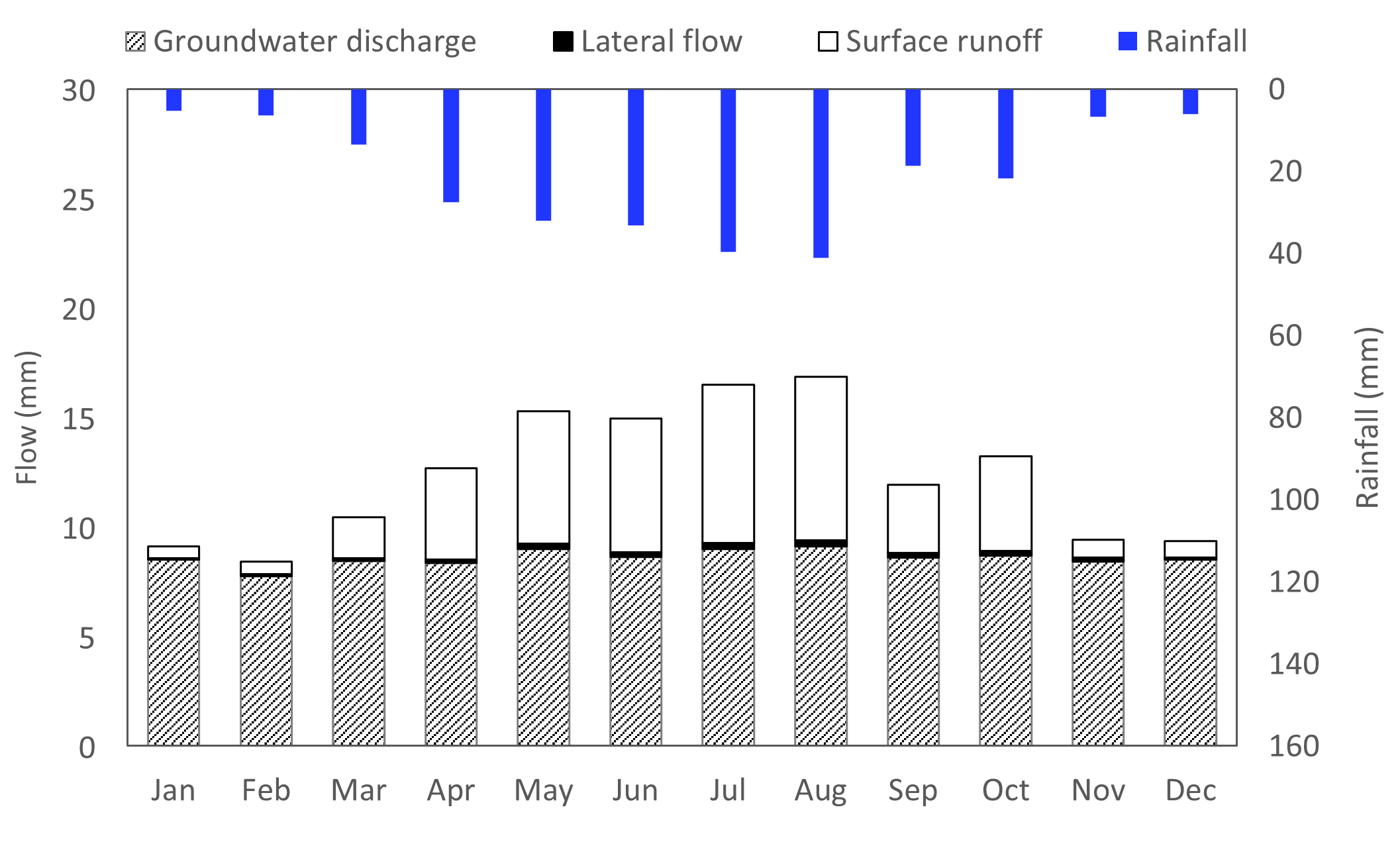
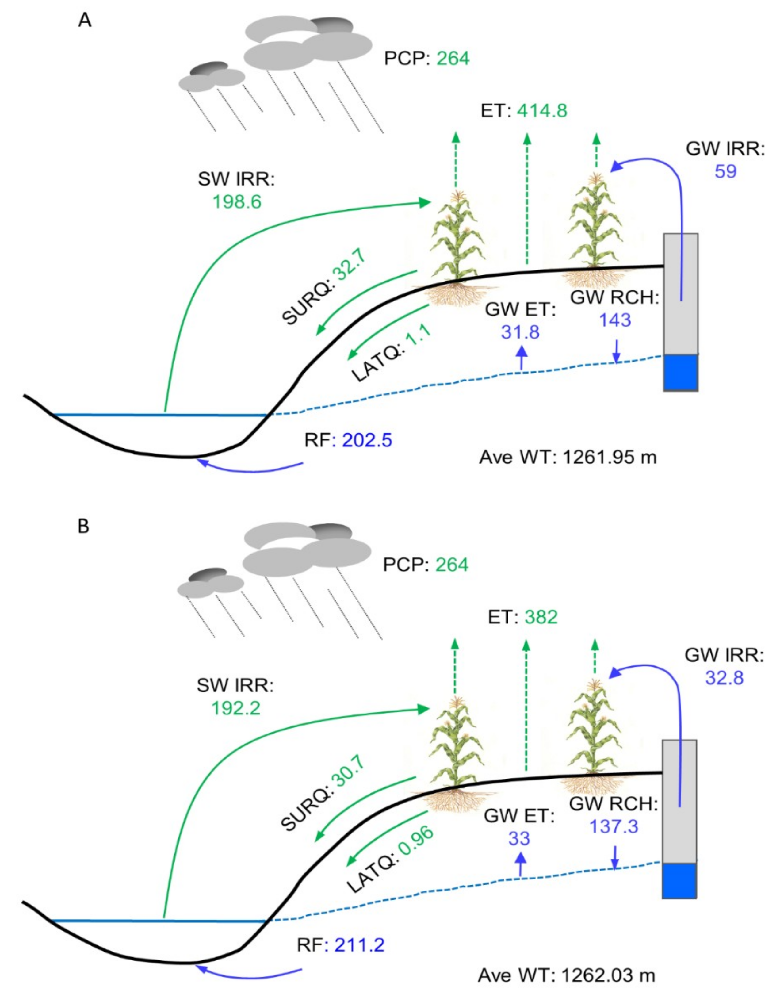
Results are first shown to demonstrate the relative flow components in the irrigated watershed. Figure 5 shows the partitioning of monthly average water yield (mm) to the river network calculated by SWAT-MODFLOW. For this study region, the amount of water entering the Arkansas River and its tributaries is dominated by groundwater discharge (74–97%), followed by surface runoff (2–25%) and lateral flow (less than 1%), which matches with the SWAT modeling results from [67]. Figure 6A gives the main components of average annual water budget, with depths of changing calculated by dividing by the area of the watershed. Surface water (198.6 mm) makes a higher contribution to irrigation than well pumping (59 mm) as the input source of irrigation water in the district [12]. Evapotranspiration is the most important output, with an average depth of 414.8 mm. It could be found out that the surface water and groundwater interactions are very strong. Water yield to the stream is dominated by return flow (202.5 mm), which accounts for 86% of the water yield.
4.2. Streamflow
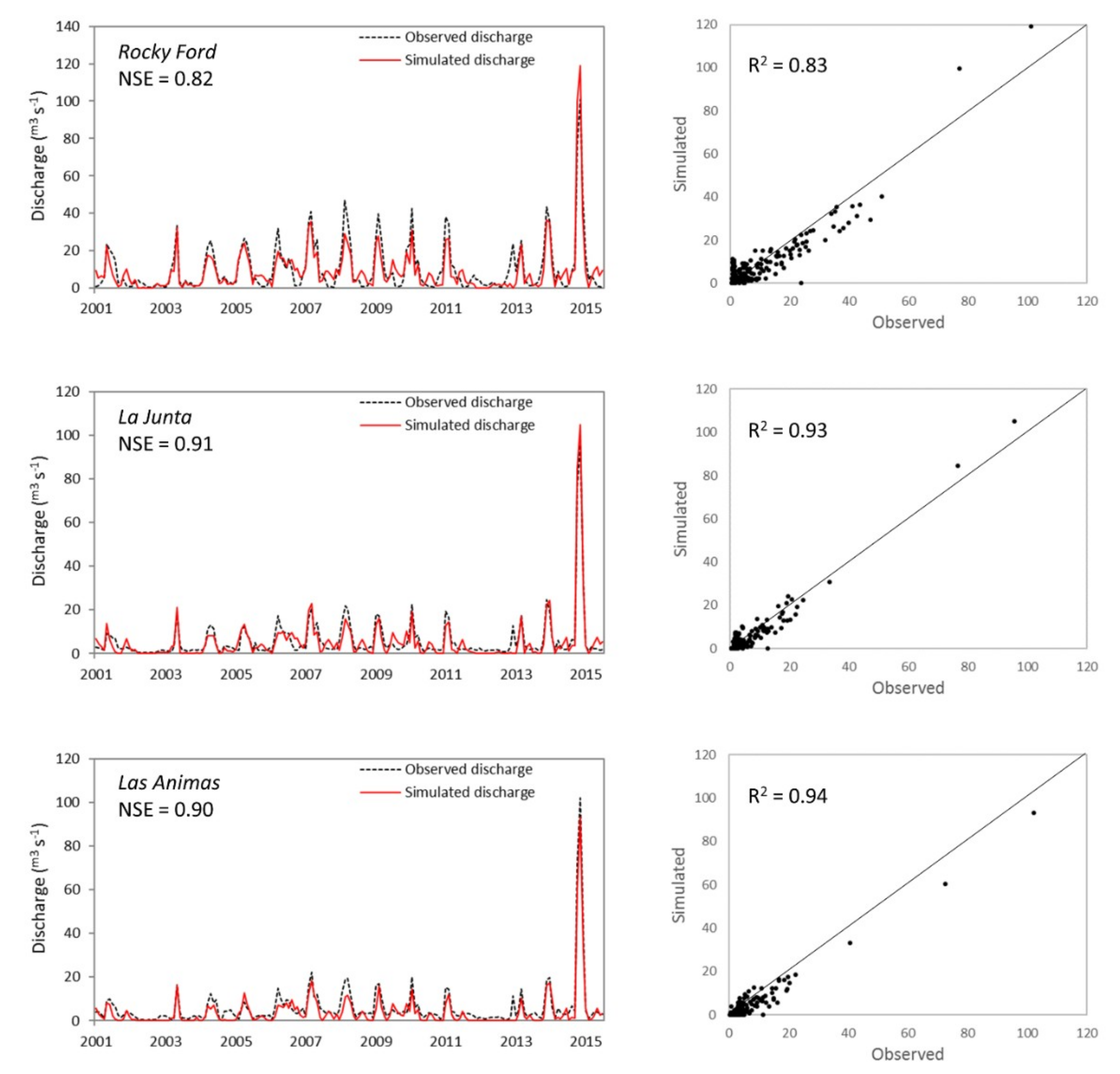
The monthly streamflow comparison between observed and simulated results along the Arkansas River at the stream gauges of Rocky Ford, La Junta, and Las Animas are shown in Figure 7. Overall, the model is able to capture the seasonal flow patterns very well. A statistical comparison of simulated streamflow at five gauging stations are given in Table 2. The values for monthly streamflow are considered to be ‘very good’ for NSE > 0.8 and R2 > 0.85, respectively [74], but poor for the two main tributaries (Timpas Creek and Crooked Arroyo). Simulated discharge for the tributaries, which act as drains for irrigation tail-water runoff and groundwater return flows, are lower than observed streamflow, which is likely because of the difficulty of physically matching the pattern of irrigation return flow from hundreds of irrigated fields. The same issue was reported by another study [50] in their groundwater model of flow and selenium transport in the study region. Another reason for the mismatch is that the model ignores any streamflow generated from upland catchments beyond the irrigated areas, which can happen during occasional intense precipitation events.
4.3. Groundwater Elevation
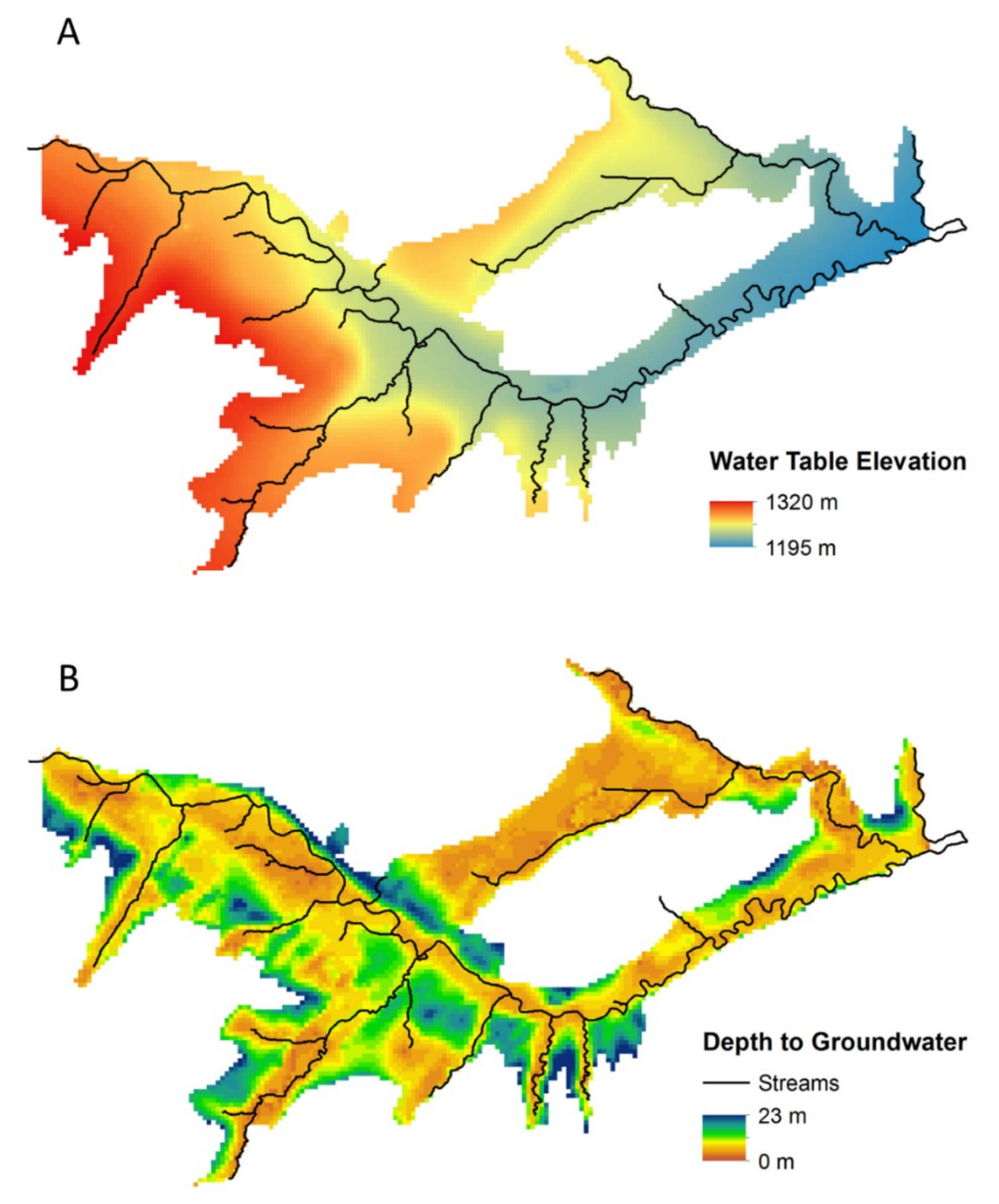
The general results of the simulated groundwater levels are shown in Figure 8. The annual average groundwater level (m) is shown in Figure 8A, with the hydraulic head ranging from 1195 m to 1320 m, decreasing from southwest to east. The spatial pattern of groundwater elevation is similar to the surface elevation, with the highest and lowest head occurring in the southwest and east regions, respectively. Figure 8B shows the cell-wise depth to the water table, which was calculated by the difference between ground surface elevation and the simulated groundwater level. It shows that the water table depths range from 0 m to 23 m, with the shallowest depths along the Arkansas River corridor and tributaries.
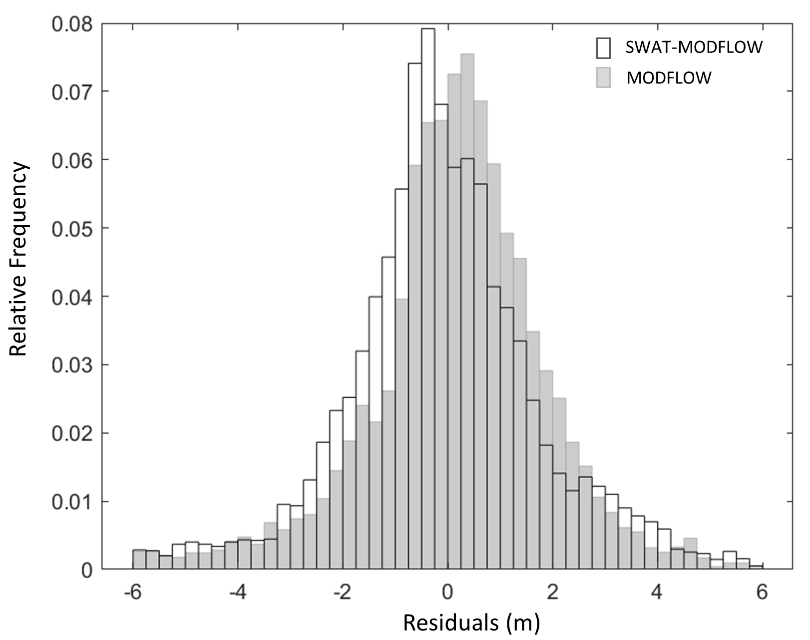
The difference between simulated and measured groundwater levels at the 89 observation wells (see Figure 2E) (a total of 9444 measurements) is summarized by a relative frequency plot of groundwater level in Figure 9. The results from the original MODFLOW model [55] also are shown (grey boxes). The average of the residuals for the SWAT-MODFLOW (−0.21 m) is similar to the original MODFLOW results (−0.22 m). The root mean square error (RMSE) of the simulated values compared to the observation values is 2.32 m. These residuals demonstrate that the model can provide an acceptable representation for the groundwater levels in the region.
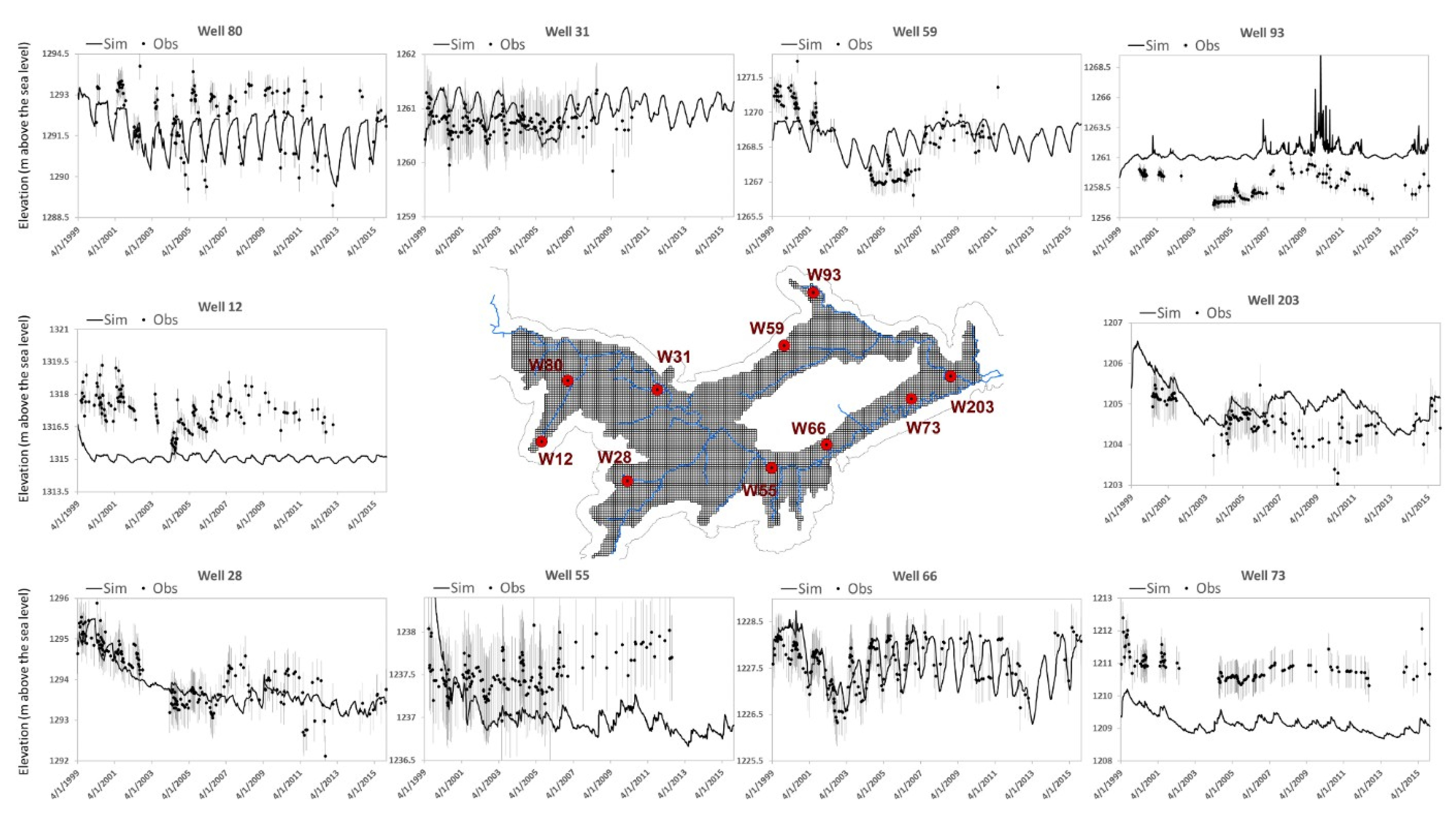
Further analysis can be performed by comparing the simulated and observed hydraulic head at 10 observation wells spread throughout the study region. Hydrographs for the time period 1999 to 2015 are shown in Figure 10. In general, simulated results are within the estimated error range of the measured head values of ±0.5 m (grey bars in Figure 10), with the errors accounting for the possible range of head values that can occur within a 250 m × 250 m area of the aquifer (i.e., the size of the grid cell). The model accurately captures the within-season and long-term trends of groundwater elevation magnitude. As can be seen in Figure 10, there are still several locations that have a significant mismatch between simulated and observed values (Well 12, Well 73, and Well 93). These discrepancies are likely due to the inaccurate recharge provided by SWAT [75,76], especially along the ungauged tributaries at the north region of the model. Moreover, it is realistic that the aquifer properties are not unique within a 250-m grid cell to induce a significant head change during certain periods. The hydraulic head estimated at the center of each cell could possibly be different from the observation value if the monitoring well is located at the edge of the grid cell.
4.4. Surface Water–Groundwater Interactions
The average simulated groundwater return flows to the Arkansas River is 1.8 × 10⁶ m3/week over the period November 2007 to December 2010, which is similar to the average value of 1.2 × 10⁶ m3/week calculated from a river water balance of the study region [77].
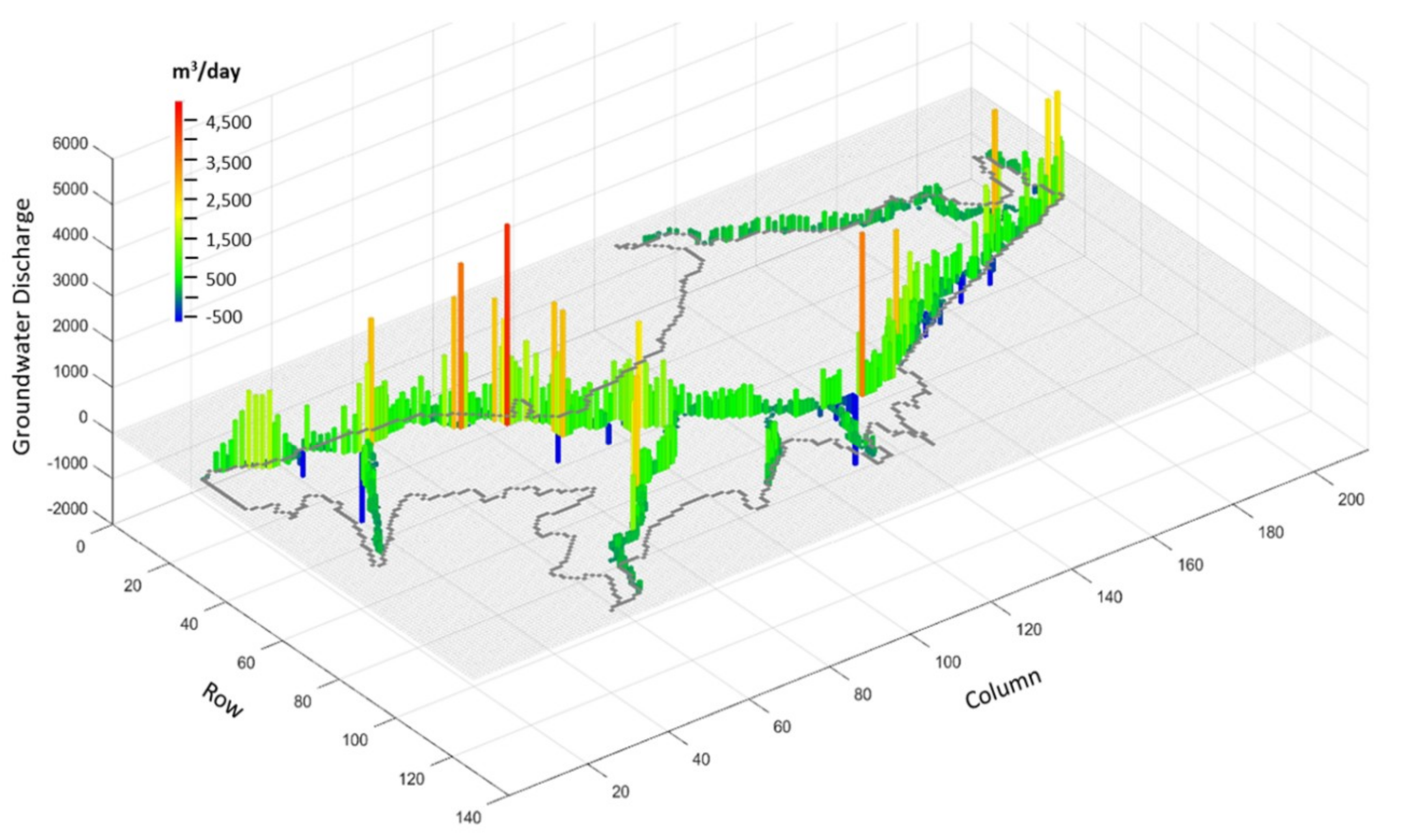
Simulated annual average surface and groundwater interactions (m3/day) for each of the 731 river cells during the 1999–2016 period are shown in Figure 11, which is important to quantify spatio-temporal patterns of surface water seepage and groundwater discharge in the watershed. Blue bars represent seepage from stream to aquifer, whereas green–yellow–red bars indicate groundwater discharge from the aquifer into the river network. It can be seen that the vast majority of surface and groundwater interactions is discharged from the aquifer to the river. The average interaction rates vary from −1611 m3/day to 7126 m3/day, with a standard deviation of 556 m3/day, which demonstrates a highly spatio-variable groundwater discharge based on different hydrological conditions.
4.5. Groundwater ET
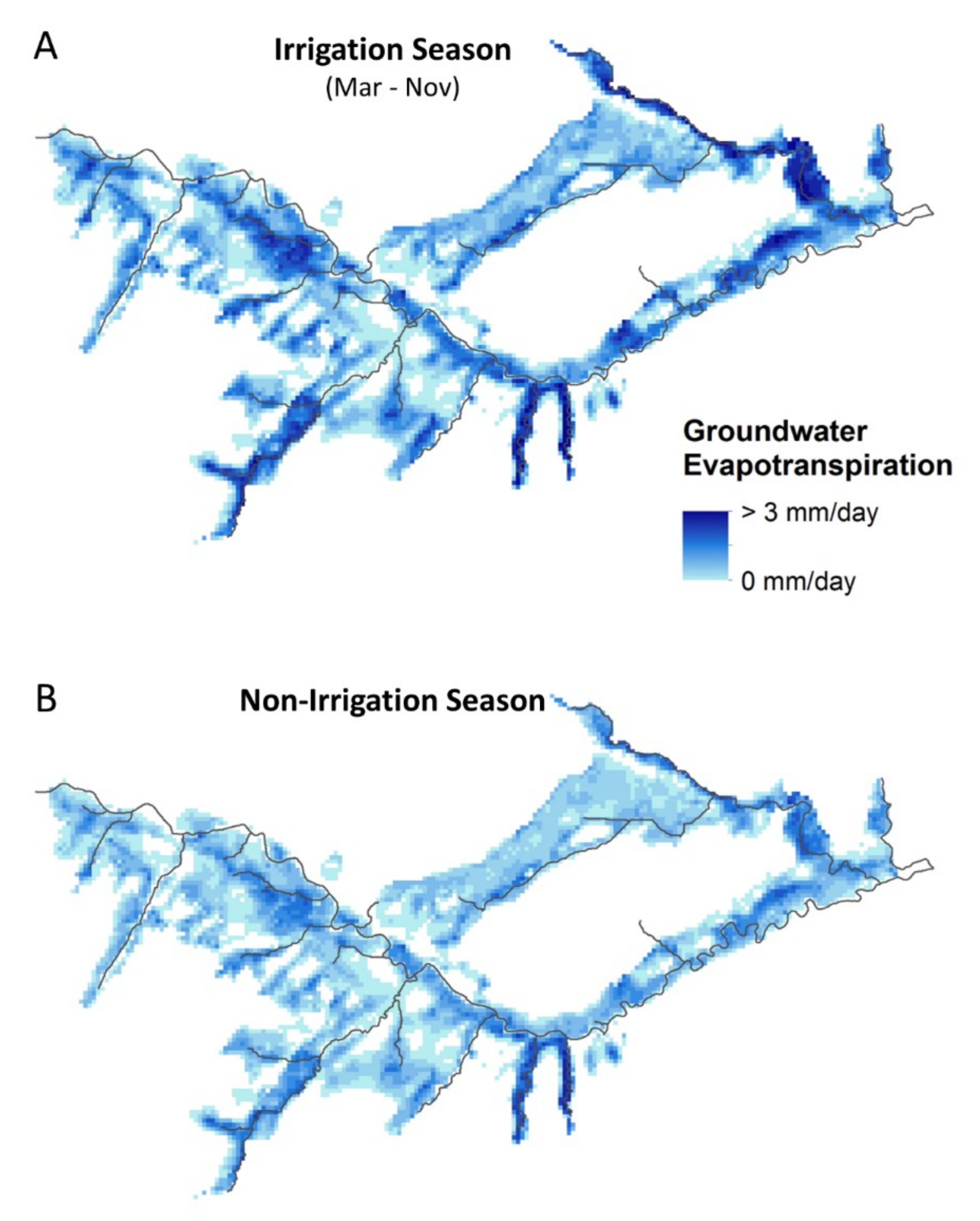
The annual average groundwater ET rate simulated by the model is 31.8 mm. The spatial pattern of the groundwater ET rate during the simulation period is shown in Figure 12, which is displayed as an average daily rate leaving the saturated zone during the irrigation season (March to November) (Figure 12A) and the non-irrigation season (Figure 12B). Groundwater ET occurs mainly along the Arkansas River corridor and tributaries. Overall, the average amount of groundwater ET is approximately constant over the simulation period, with the rates decreasing from the irrigation season to the non-irrigation season. Magnitudes and spatial patterns of groundwater ET are very similar to the results of the original MODFLOW model [55].
4.6. Crop Yield
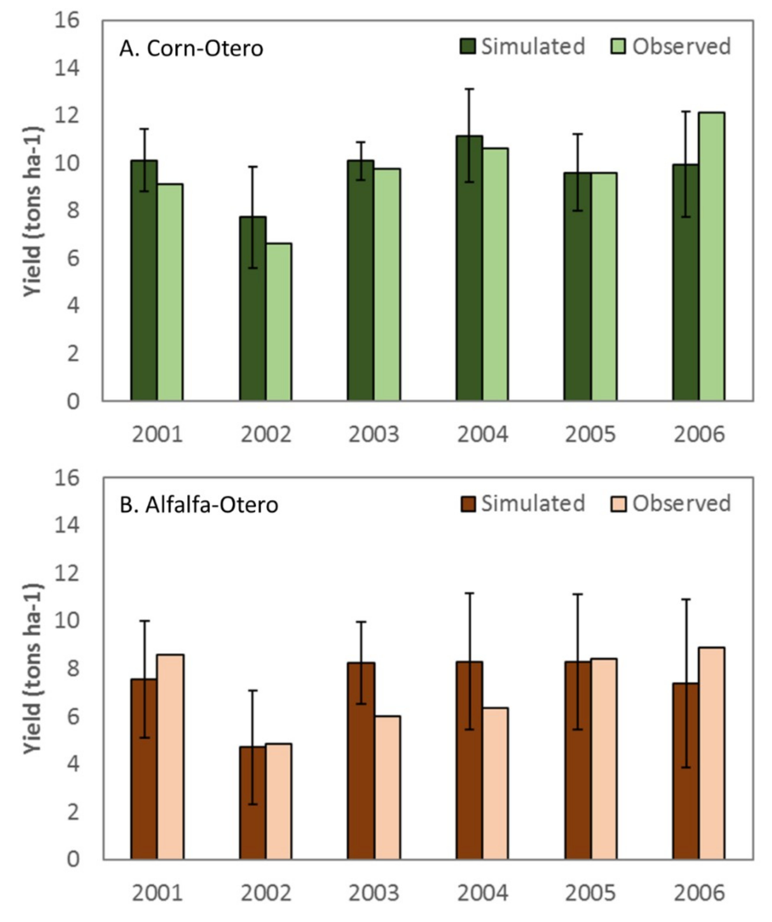
Crop yield is one of the most important factors to estimate water productivity, especially in the Colorado area [35,78]. In this study, we compared the simulated crop yields in Otero County with the NASS reported mean yields of corn and alfalfa on an annual basis, as the majority of irrigated fields are located in this county (Figure 2A). Figure 13A,B present the annual comparison of predicted and observed corn yield and alfalfa yield, respectively in Otero County for the years 2001–2006. The error bars on the plots represent the standard deviation of all the simulated values. It is shown that the model can capture the annual variation in crop yields quite well, with the annual average yield of 9.7 tons/ha and 7.4 tons/ha for corn and alfalfa, respectively. The percent bais (PBIAS) is 3.1% and 1.5% for corn yield and alfalfa yield, respectively. In this model, we assigned the management practices (e.g., crop rotation, fertilizer, harvest, and tillage) at the HRU scale according to the actual farm-scale conditions [67], which helps to improve model performance. Although the model tends to underestimate both corn and alfalfa yields in 2006 and overestimate alfalfa in 2003 and 2004, the objective is to capture the regional trends in total crop yield.
4.7. Quantifying the Impacts of the Irrigation on System Responses
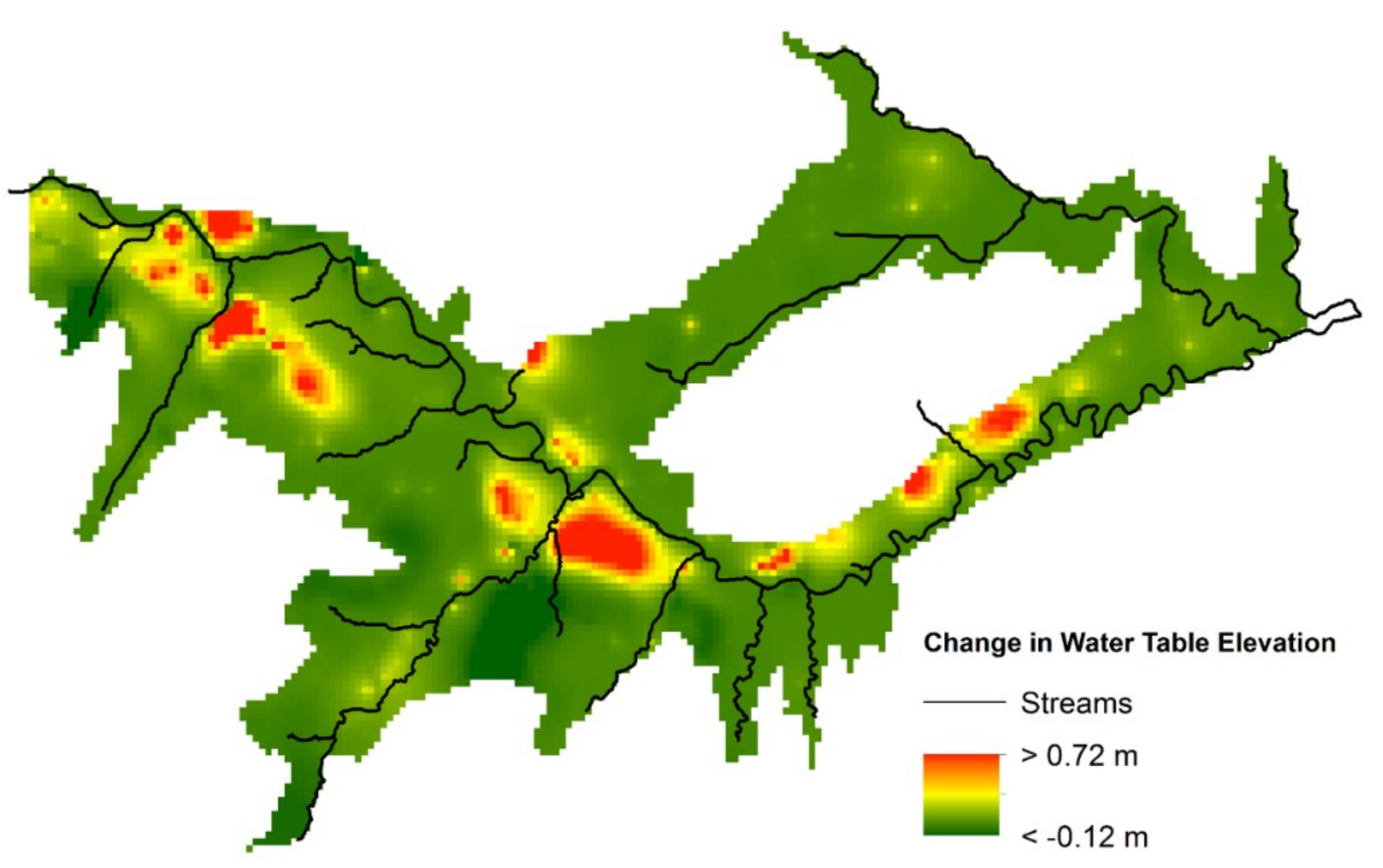
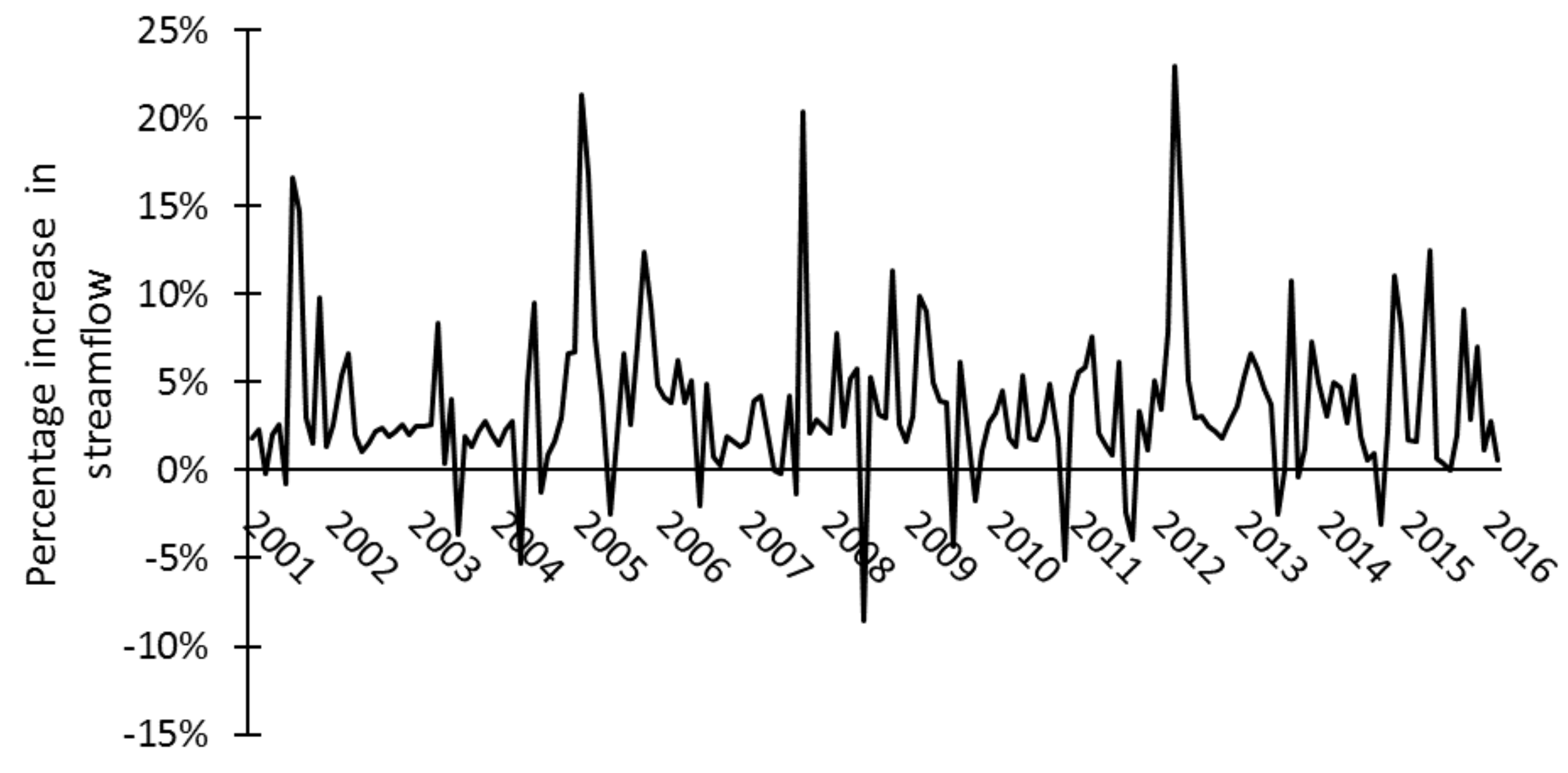
Figure 6B gives the main components of the water budget for the reduced irrigation scenario. As expected, surface water and groundwater irrigation decreases (6.4 mm and 26.2 mm), respectively, in the control of water stress threshold and pumping rate and less consumptive use by crops. As a result of the lower irrigation application rates, the ET flux is decreased by 32.8 and the surface runoff is decreased by 2 mm, which also decreases recharge by 5.7 mm. However, the water table is influenced more by the decrease in pumping than the decrease in recharge, resulting in higher water table elevation, which drives more groundwater into the river network (i.e., increase in return flow from 202.5 mm to 211.2 mm, 4.3%). This is also demonstrated by the annual average increase in groundwater elevation (Figure 14), which is calculated by taking the difference between the reduced irrigation scenario and the baseline scenario. As expected, the water table increases in areas of pumping wells (see Figure 2E) due to the strong causal relationship between pumping and sustained shallow water tables, but decreases in areas of surface water irrigation due to the decrease in recharge. The overall average increase in water table elevation is 65 mm (Figure 6), thus leading to the increase in groundwater return flow (202.5 mm to 211.2 mm). The percentage increase in streamflow in the Arkansas River is shown in Figure 15, with the increase occurring due to less water diverted for surface water irrigation and more groundwater return flow.
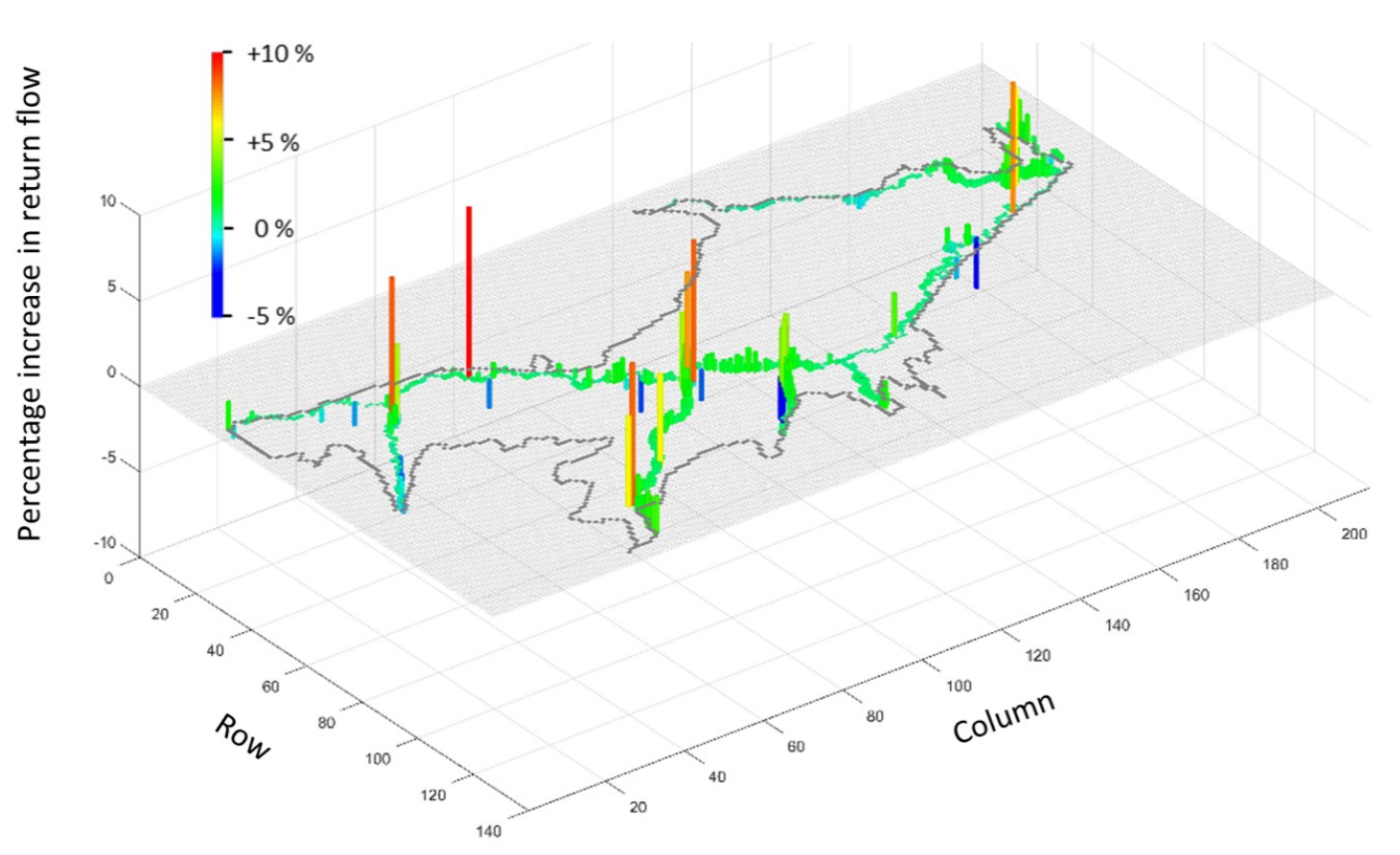
The percentage increase in return flow for each of the river cells during the simulation period is shown in Figure 16, with green–yellow–red bars representing groundwater return flow. It can be seen from this figure that the majority of river cells are gaining return flows for the reduced irrigation scenario, with the highest percentage increase of 31%. This is an important result—implementing a basin-wide decrease in irrigation water for both surface water irrigation and groundwater irrigation does not necessarily improve waterlogging occurrence, and can actually increase the groundwater loading of salts, nitrate, phosphorus, and trace elements (selenium, uranium) due to an increase in groundwater return flow. This may be due to the close proximity of the pumping wells to the Arkansas River; therefore, the areas that control groundwater discharge to the Arkansas River have higher water tables than those in the baseline scenarios. However, in general, a targeted approach must be taken that focuses on decreasing surface water irrigation and allowing the groundwater pumps to continue operation. This will maintain deep water tables and decrease the recharge, therefore preventing waterlogging.
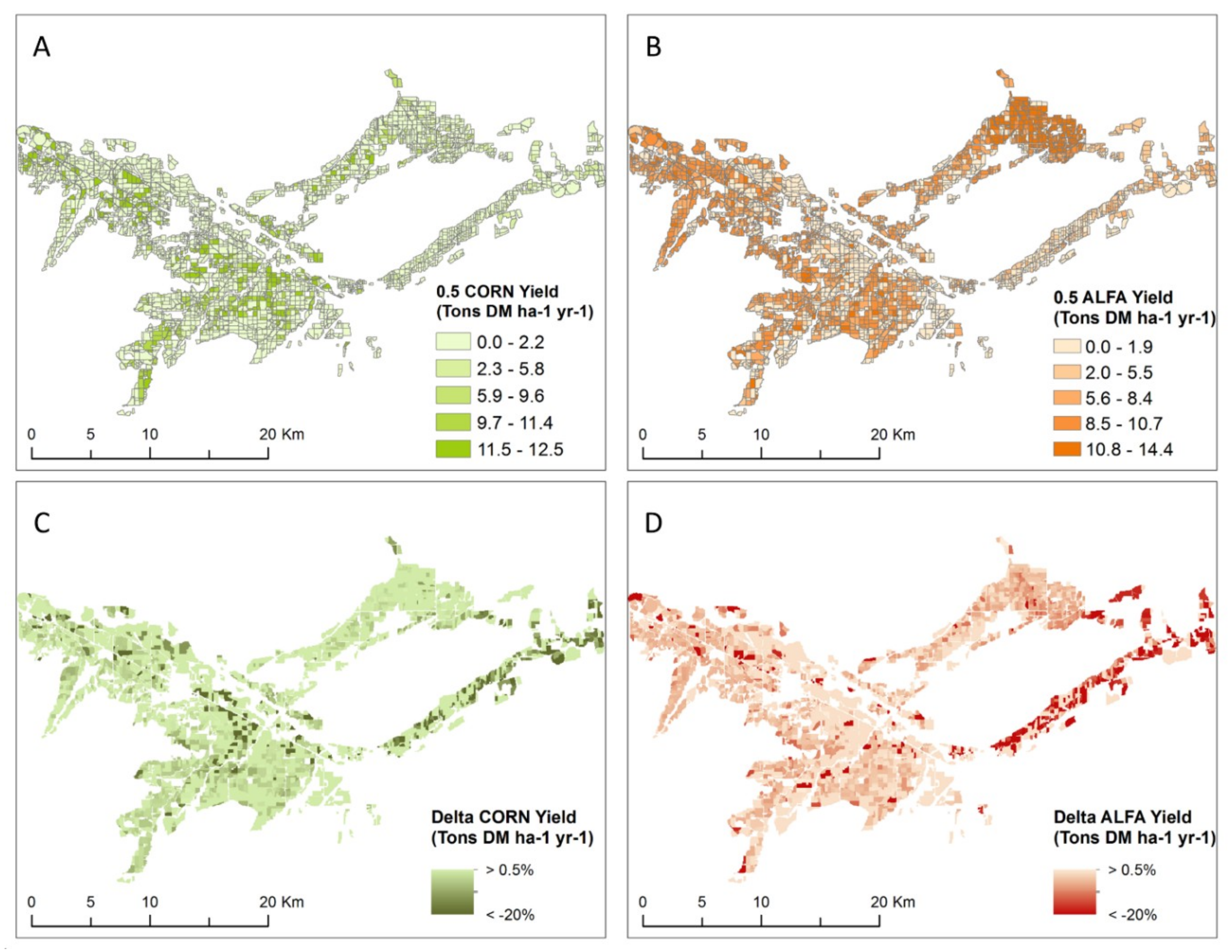
To complete the analysis of trade-offs, the change in crop yield between the baseline scenario and the reduced irrigation scenarios must be quantified. For the multi-year average assessment, the average yield under the reduced irrigation scenario for the entire irrigated fields is 8.9 tons/ha and 6.7 tons/ha for corn and alfalfa, respectively. The average production for these corn and alfalfa crops is shown by an HRU in Figure 17. Two types of assessments are conducted over the 18-year simulation period to compare the average crop production under the reduced irrigation condition: (1) annual spatial yield (Figure 17A,B) and (2) yield reduction between the reduced irrigation scenario and the baseline scenario (Figure 17C,D). We observed that corn has a higher yield in the central part of the study region, while the alfalfa yield has a wider spread and shows high yield in the north region. In general, the reduced irrigation scenario leads to a widespread reduction in crop yield, with a few locations of increased crop yield. The average reductions in crop yield are 8.8% and 9.2% for corn and alfalfa, respectively. Figure 17C,D shows that 5.9% and 6.3% of the corn field and alfalfa field experienced more than 20% reductions in crop production, respectively. Results also show that some fields do not have significant crop yield change under the irrigation scenario. Those fields could likely receive the extra irrigation water that is saved by the reduced surface water triggered by auto-irrigation water stress, so that the crop yield could decrease more slowly when the irrigation amount approaches the crop water demand [79,80].
5. Summary and Conclusions
This paper presents the application of a new version of the SWAT-MODFLOW code [56] to a 732 km2 irrigated stream–aquifer system in the Lower Arkansas River Valley, Colorado. The model accounts for the influence of irrigation applications, canal diversions, earthen canal seepage, and groundwater pumping. The model provides a detailed description of surface and groundwater flow processes, thereby enabling a detailed description of watershed processes such as surface runoff, ET, infiltration, soil lateral flow, recharge, groundwater ET, three-dimensional groundwater flow in a heterogeneous aquifer system with sources and sinks, spatio-temporal groundwater and surface water interactions (e.g., groundwater discharge to the river network), and streamflow. Model performance was tested against stream discharge, groundwater levels, groundwater return flow, and crop yield. Therefore, this paper serves as a guideline for implementing SWAT-MODFLOW models in irrigated watersheds wherein streamflow is influenced by groundwater-surface water interactions.
The model was used to explore the effects of reducing irrigation rates on hydrologic responses (surface runoff, recharge, water table elevation, return flows, streamflow) and crop yield. The results reveal that jointly decreasing surface water irrigation and groundwater irrigation yields an overall increase in water table elevation, with the decrease in pumping having a stronger influence than the decrease in recharge on groundwater levels. The higher groundwater levels enhance the prospect of waterlogging and salinization, and increase the groundwater gradient to the river, increasing the groundwater discharge rates to the Arkansas River, and resulting in an increase in the loading of salts and pollutants to the stream. This will be addressed in future studies using a coupled surface/subsurface nutrient transport model. In addition, 8.8% (corn) and 9.2% (alfalfa) crop reduction are observed in the reduced irrigation scenario.
This study points to the need for targeted irrigation reduction scenarios that will decrease shallow water tables while also maintaining crop yields. It is likely that this will be targeting surface water irrigation for irrigation reduction, with groundwater pumping for irrigation allowed to continue to (1) maintain the basin-wide crop yield and (2) maintain adequately deep water tables to prevent waterlogging. The results discussed here only concern system hydrological responses. The nutrient fate and transport, as well as plausible best management practices for controlling contaminant pollution need to be addressed in intensively irrigated stream–aquifer systems in order to provide water resources managers with a detailed description of the alternative management options.
Author Contributions
X.W. and R.T.B. conceived and designed this research; X.W. wrote the paper; R.T.B. provided professional guidance and edited the paper.
Funding
This work was supported by a grant from the Agriculture and Food Research Initiative of the USDA National Institute of Food and Agriculture, grant number #2012-67003-19904.
Conflicts of Interest
The authors declare no conflict of interest.
References
- Lobell, D.B.; Lesch, S.M.; Corwin, D.L.; Ulmer, M.G.; Anderson, K.A.; Potts, D.J.; Doolittle, J.A.; Matos, M.R.; Baltes, M.J. Regional-scale Assessment of Soil Salinity in the Red River Valley Using Multi-year MODIS EVI and NDVI. J. Environ. Qual. 2010, 39, 35–41. [Google Scholar] [CrossRef] [PubMed] [Green Version]
- Törnqvist, R.; Jarsjö, J. Water Savings Through Improved Irrigation Techniques: Basin-Scale Quantification in Semi-Arid Environments. Water Resour. Manag. 2012, 26, 949–962. [Google Scholar] [CrossRef]
- Martin-Carrasco, F.; Garrote, L.; Iglesias, A.; Mediero, L. Diagnosing Causes of Water Scarcity in Complex Water Resources Systems and Identifying Risk Management Actions. Water Resour. Manag. 2013, 27, 1693–1705. [Google Scholar] [CrossRef]
- Robertson, A.D.; Zhang, Y.; Sherrod, L.A.; Rosenzweig, S.T.; Ma, L.; Ahuja, L.; Schipanski, M.E. Climate Change Impacts on Yields and Soil Carbon in Row Crop Dryland Agriculture. J. Environ. Qual. 2018, 47, 684–694. [Google Scholar] [CrossRef] [PubMed] [Green Version]
- Droogers, P.; Bastiaanssen, W. Irrigation performance using hydrological and remote sensing modeling. J. Irrig. Drain. Eng. 2002, 128, 11–18. [Google Scholar] [CrossRef]
- Cai, X.; McKinney, D.C.; Rosegrant, M.W. Sustainability analysis for irrigation water management in the Aral Sea region. Agric. Syst. 2003, 76, 1043–1066. [Google Scholar] [CrossRef] [Green Version]
- Niemann, J.D.; Lehman, B.M.; Gates, T.K.; Hallberg, N.U.; Elhaddad, A. Impact of Shallow Groundwater on Evapotranspiration Losses from Uncultivated Land in an Irrigated River Valley. J. Irrig. Drain. Eng. 2011, 137, 501–512. [Google Scholar] [CrossRef]
- Pokhrel, Y.N.; Koirala, S.; Yeh, P.J.-F.; Hanasaki, N.; Longuevergne, L.; Kanae, S.; Oki, T. Incorporation of groundwater pumping in a global Land Surface Model with the representation of human impacts. Water Resour. Res. 2015, 51, 78–96. [Google Scholar] [CrossRef]
- Aliyari, F.; Bailey, R.T.; Tasdighi, A.; Dozier, A.; Arabi, M.; Zeiler, K. Coupled SWAT-MODFLOW model for large-scale mixed agro-urban river basins. Environ. Model. Softw. 2019, 115, 200–210. [Google Scholar] [CrossRef]
- Pimentel, D.; Houser, J.; Preiss, E.; White, O.; Fang, H.; Mesnick, L.; Barsky, T.; Tariche, S.; Schreck, J.; Alpert, S. Water resources: Agriculture, the environment, and society. BioScience 1997, 47, 97–106. [Google Scholar] [CrossRef]
- Scanlon, B.R.; Jolly, I.; Sophocleous, M.; Zhang, L. Global impacts of conversions from natural to agricultural ecosystems on water resources: Quantity versus quality. Water Resour. Res. 2007. [Google Scholar] [CrossRef]
- Gates, T.K.; Garcia, L.A.; Hemphill, R.A.; Morway, E.D.; Elhaddad, A. Irrigation Practices, Water Consumption, & Return Flows in Colorado’s Lower Arkansas River Valley: Field and Model Investigations. In Technical Report No. TR12-10; Colorado Agricultural Experiment Station: Fort Collins, CO, USA, 2012. [Google Scholar]
- Tanji, K.K.; Kielen, N.C. Agricultural Drainage Water Management in Arid and Semi-ARID areas; FAO: Rome, Italy, 2002. [Google Scholar]
- Burkhalter, J.P.; Gates, T.K. Agroecological Impacts from Salinization and Waterlogging in an Irrigated River Valley. J. Irrig. Drain. Eng. 2005, 131, 197–209. [Google Scholar] [CrossRef]
- Qureshi, A.S.; McCornick, P.G.; Sarwar, A.; Sharma, B.R. Challenges and Prospects of Sustainable Groundwater Management in the Indus Basin, Pakistan. Water Resour. Manag. 2010, 24, 1551–1569. [Google Scholar] [CrossRef]
- Borah, K.K.; Bera, M. Watershed-Scale Hydrologic and Nonpoint-Source Pollution Models: Review of Mathematical Bases. Trans. ASAE 2003, 46, 1553–1566. [Google Scholar] [CrossRef]
- Schoumans, O.F.; Silgram, M.; Walvoort, D.J.J.; Groenendijk, P.; Bouraoui, F.; Andersen, H.E.; Porto, A.L.; Reisser, H.; Gall, G.L.; Anthony, S.; et al. Evaluation of the difference of eight model applications to assess diffuse annual nutrient losses from agricultural land. J. Environ. Monit. 2009, 11, 540–553. [Google Scholar] [CrossRef]
- Devia, G.K.; Ganasri, B.P.; Dwarakish, G.S. A Review on Hydrological Models. Aquat. Procedia 2015, 4, 1001–1007. [Google Scholar] [CrossRef]
- Francesconi, W.; Srinivasan, R.; Pérez-Miñana, E.; Willcock, S.P.; Quintero, M. Using the Soil and Water Assessment Tool (SWAT) to model ecosystem services: A systematic review. J. Hydrol. 2016, 535, 625–636. [Google Scholar] [CrossRef]
- Young, R.A.; Onstad, C.A.; Bosch, D.D.; Anderson, W.P. AGNPS: A nonpoint-source pollution model for evaluating agricultural watersheds. J. Soil Water Conserv. 1989, 44, 168–173. [Google Scholar]
- Bicknell, B.R.; Imhoff, J.C.; Kittle, J.L., Jr; Donigian, A.S., Jr; Johanson, R.C. Hydrologic Simulation Program-FORTRAN (HSPF): User’s Manual for version 11 1997. In Environmental Protection Agency Report No. EPA/600/R-97/080; US Environmental Protection Agency: Athens, Ga, USA, 1997. [Google Scholar]
- Charley, W.; Pabst, A.; Peters, J. The Hydrologic Modeling System (HEC-HMS): Design and Development Issues; Hydrologic Engineering Center: Davis, CA, USA, 1995. [Google Scholar]
- Woolhiser, D.A.; Smith, R.E.; Goodrich, D.C. KINEROS: A Kinematic Runoff and Erosion Model: Documentation and User Manual; US Department of Agriculture, Agricultural Research Service: Washington, DC, USA, 1990.
- Arnold, J.G.; Srinivasan, R.; Muttiah, R.S.; Williams, J.R. Large Area Hydrologic Modeling and Assessment Part I: Model Development1. JAWRA J. Am. Water Resour. Assoc. 1998, 34, 73–89. [Google Scholar] [CrossRef]
- Krysanova, V.; Wechsung, F.; Arnold, J.; Srinivasan, R.; Williams, J. SWIM (Soil and Water Integrated Model); Potsdam-Institut fuer Klimafolgenforschung (PIK): Potsdam, Germany, 2000; p. 239. [Google Scholar]
- Ogden, F.L.; Julien, P.Y.; Singh, V.; Frevert, D. CASC2D: A Two-Dimensional, Physically-Based, Hortonian Hydrologic Model; Water Resources Publications: Littleton, CO, USA, 2002. [Google Scholar]
- Gassman, P.W.; Reyes, M.R.; Green, C.H.; Arnold, J.G. The soil and water assessment tool: Historical development, applications, and future research directions. Trans. ASABE 2007, 50, 1211–1250. [Google Scholar] [CrossRef]
- Chiang, L.; Chaubey, I.; Gitau, M.W.; Arnold, J.G. Differentiating Impacts of Land Use Changes from Pasture Management in a CEAP Watershed Using the SWAT Model. Trans. ASABE 2010, 53, 1569–1584. [Google Scholar] [CrossRef]
- Ghebremichael, L.T.; Veith, T.L.; Watzin, M.C. Determination of Critical Source Areas for Phosphorus Loss: Lake Champlain Basin, Vermont. Trans. ASABE 2010, 53, 1595–1604. [Google Scholar] [CrossRef]
- Strehmel, A.; Schmalz, B.; Fohrer, N. Evaluation of Land Use, Land Management and Soil Conservation Strategies to Reduce Non-Point Source Pollution Loads in the Three Gorges Region, China. Environ. Manag. 2016, 58, 906–921. [Google Scholar] [CrossRef] [PubMed]
- Jang, S.S.; Ahn, S.R.; Kim, S.J. Evaluation of executable best management practices in Haean highland agricultural catchment of South Korea using SWAT. Agric. Water Manag. 2017, 180, 224–234. [Google Scholar] [CrossRef]
- Jayakrishnan, R.; Srinivasan, R.; Santhi, C.; Arnold, J.G. Advances in the application of the SWAT model for water resources management. Hydrol. Process. 2005, 19, 749–762. [Google Scholar] [CrossRef]
- Ullrich, A.; Volk, M. Application of the Soil and Water Assessment Tool (SWAT) to predict the impact of alternative management practices on water quality and quantity. Agric. Water Manag. 2009, 96, 1207–1217. [Google Scholar] [CrossRef]
- Wang, R.; Bowling, L.C.; Cherkauer, K.A. Estimation of the effects of climate variability on crop yield in the Midwest USA. Agr. Forest Meteorol. 2016, 216, 141–156. [Google Scholar] [CrossRef] [Green Version]
- Ahmadzadeh, H.; Morid, S.; Delavar, M.; Srinivasan, R. Using the SWAT model to assess the impacts of changing irrigation from surface to pressurized systems on water productivity and water saving in the Zarrineh Rud catchment. Agric. Water Manag. 2016, 175, 15–28. [Google Scholar] [CrossRef]
- Fleckenstein, J.H.; Krause, S.; Hannah, D.M.; Boano, F. Groundwater-surface water interactions: New methods and models to improve understanding of processes and dynamics. Adv. Water Resour. 2010, 33, 1291–1295. [Google Scholar] [CrossRef]
- Spruill, C.A.; Workman, S.R.; Taraba, J.L. Simulation of daily and monthly stream discharge from small watersheds using the SWAT model. Trans. ASAE 2000, 43, 1431–1439. [Google Scholar] [CrossRef]
- Chu, T.W.; Shirmohammadi, A. Evaluation of the SWAT model’s hydrology component in the piedmont physiographic region of Maryland. Trans. ASAE 2004, 47, 1057. [Google Scholar] [CrossRef]
- Paniconi, C.; Marrocu, M.; Putti, M.; Verbunt, M. Newtonian nudging for a Richards equation-based distributed hydrological model. Adv. Water Resour. 2003, 26, 161–178. [Google Scholar] [CrossRef]
- Markstrom, S.L.; Niswonger, R.G.; Regan, R.S.; Prudic, D.E.; Barlow, P.M. GSFLOW-Coupled Ground-Water and Surface-Water FLOW Model Based on the Integration of the Precipitation-Runoff Modeling System (PRMS) and the Modular Ground-Water Flow Model (MODFLOW-2005); U.S. Geological Survey: Reston, VI, USA, 2008.
- Kollet, S.J.; Maxwell, R.M. Capturing the influence of groundwater dynamics on land surface processes using an integrated, distributed watershed model. Water Resour. Res. 2008. [Google Scholar] [CrossRef]
- Therrien, R.; McLaren, R.G.; Sudicky, E.A.; Panday, S.M. HydroGeoSphere: A Three-Dimensional Numerical Model Describing Fully-Integrated Subsurface and Surface Flow and Solute Transport; Groundwater Simulations Group, University of Waterloo: Waterloo, ON, Canada, 2010. [Google Scholar]
- Kolditz, O.; Bauer, S.; Bilke, L.; Böttcher, N.; Delfs, J.O.; Fischer, T.; Görke, U.J.; Kalbacher, T.; Kosakowski, G.; McDermott, C.I.; et al. OpenGeoSys: An open-source initiative for numerical simulation of thermo-hydro-mechanical/chemical (THM/C) processes in porous media. Environ. Earth Sci. 2012, 67, 589–599. [Google Scholar] [CrossRef]
- Refsgaard, J.C. Parameterisation, calibration and validation of distributed hydrological models. J. Hydrol. 1997, 198, 69–97. [Google Scholar] [CrossRef]
- Wu, X.; Zheng, Y.; Wu, B.; Tian, Y.; Han, F.; Zheng, C. Optimizing conjunctive use of surface water and groundwater for irrigation to address human-nature water conflicts: A surrogate modeling approach. Agric. Water Manag. 2016, 163, 380–392. [Google Scholar] [CrossRef]
- Larsen, M.A.D.; Rasmussen, S.H.; Drews, M.; Butts, M.B.; Christensen, J.H.; Refsgaard, J.C. Assessing the influence of groundwater and land surface scheme in the modelling of land surface–atmosphere feedbacks over the FIFE area in Kansas, USA. Environ. Earth Sci. 2016, 75, 130. [Google Scholar] [CrossRef]
- Ward, F.A.; Booker, J.F.; Michelsen, A.M. Integrated Economic, Hydrologic, and Institutional Analysis of Policy Responses to Mitigate Drought Impacts in Rio Grande Basin. J. Water Resour. Plan. Manag. 2006, 132, 488–502. [Google Scholar] [CrossRef] [Green Version]
- Scibek, J.; Allen, D.M.; Cannon, A.J.; Whitfield, P.H. Groundwater–surface water interaction under scenarios of climate change using a high-resolution transient groundwater model. J. Hydrol. 2007, 333, 165–181. [Google Scholar] [CrossRef]
- Ahrends, H.; Mast, M.; Rodgers, Ch.; Kunstmann, H. Coupled hydrological–economic modelling for optimised irrigated cultivation in a semi-arid catchment of West Africa. Environ. Model. Softw. 2008, 23, 385–395. [Google Scholar] [CrossRef]
- Shultz, C.D.; Bailey, R.T.; Gates, T.K.; Heesemann, B.E.; Morway, E.D. Simulating selenium and nitrogen fate and transport in coupled stream-aquifer systems of irrigated regions. J. Hydrol. 2018, 560, 512–529. [Google Scholar] [CrossRef]
- Wei, X.; Bailey, R.T.; Records, R.M.; Wible, T.C.; Arabi, M. Comprehensive simulation of nitrate transport in coupled surface-subsurface hydrologic systems using the linked SWAT-MODFLOW-RT3D model. Environ. Model. Softw. 2018. [Google Scholar] [CrossRef]
- Bauer, P.; Gumbricht, T.; Kinzelbach, W. A regional coupled surface water/groundwater model of the Okavango Delta, Botswana. Water Resour. Res. 2006. [Google Scholar] [CrossRef]
- Anibas, C.; Verbeiren, B.; Buis, K.; Chormański, J.; De Doncker, L.; Okruszko, T.; Meire, P.; Batelaan, O. A hierarchical approach on groundwater-surface water interaction in wetlands along the upper Biebrza River, Poland. Hydrol. Earth Syst. Sci. 2012, 16, 2329–2346. [Google Scholar] [CrossRef] [Green Version]
- Harbaugh, A.W. MODFLOW-2005, the US Geological Survey modular ground-water model: The ground-water flow process; US Department of the Interior, US Geological Survey: Reston, VA, USA, 2005.
- Morway, E.D.; Gates, T.K.; Niswonger, R.G. Appraising options to reduce shallow groundwater tables and enhance flow conditions over regional scales in an irrigated alluvial aquifer system. J. Hydrol. 2013, 495, 216–237. [Google Scholar] [CrossRef]
- Bailey, R.T.; Wible, T.C.; Arabi, M.; Records, R.M.; Ditty, J. Assessing regional-scale spatio-temporal patterns of groundwater–surface water interactions using a coupled SWAT-MODFLOW model. Hydrol. Process. 2016, 30, 4420–4433. [Google Scholar] [CrossRef]
- Geza, M.; McCray, J.E. Effects of soil data resolution on SWAT model stream flow and water quality predictions. J. Environ. Manag. 2008, 88, 393–406. [Google Scholar] [CrossRef]
- Srinivasan, R.; Zhang, X.; Arnold, J. SWAT ungauged: Hydrological budget and crop yield predictions in the Upper Mississippi River Basin. Trans. ASABE 2010, 53, 1533–1546. [Google Scholar] [CrossRef]
- Zhang, X.; Srinivasan, R.; Arnold, J.; Izaurralde, R.C.; Bosch, D. Simultaneous calibration of surface flow and baseflow simulations: A revisit of the SWAT model calibration framework. Hydrol. Process. 2011, 25, 2313–2320. [Google Scholar] [CrossRef]
- Garg, K.K.; Bharati, L.; Gaur, A.; George, B.; Acharya, S.; Jella, K.; Narasimhan, B. Spatial mapping of agricultural water productivity using the SWAT model in Upper Bhima Catchment, India. Irrig. Drain. 2012, 61, 60–79. [Google Scholar] [CrossRef]
- Baker, T.J.; Miller, S.N. Using the Soil and Water Assessment Tool (SWAT) to assess land use impact on water resources in an East African watershed. J. Hydrol. 2013, 486, 100–111. [Google Scholar] [CrossRef]
- Kundu, D.; Vervoort, R.W.; Ogtrop, F.F. The value of remotely sensed surface soil moisture for model calibration using SWAT. Hydrol. Process. 2017, 31, 2764–2780. [Google Scholar] [CrossRef]
- Niswonger, R.G.; Panday, S.; Ibaraki, M. MODFLOW-NWT, a Newton formulation for MODFLOW-2005. US Geol. Surv. Tech. Methods 2011, 6, 44. [Google Scholar]
- Sophocleous, M.; Perkins, S.P. Methodology and application of combined watershed and ground-water models in Kansas. J. Hydrol. 2000, 236, 185–201. [Google Scholar] [CrossRef]
- Kim, N.W.; Chung, I.M.; Won, Y.S.; Arnold, J.G. Development and application of the integrated SWAT–MODFLOW model. J. Hydrol. 2008, 356, 1–16. [Google Scholar] [CrossRef]
- Guzman, J.A.; Moriasi, D.N.; Gowda, P.H.; Steiner, J.L.; Starks, P.J.; Arnold, J.G.; Srinivasan, R. A model integration framework for linking SWAT and MODFLOW. Environ. Model. Softw. 2015, 73, 103–116. [Google Scholar] [CrossRef]
- Wei, X.; Bailey, R.T.; Tasdighi, A. Using the SWAT Model in Intensively Managed Irrigated Watersheds: Model Modification and Application. J. Hydrol. Eng. 2018, 23, 04018044. [Google Scholar] [CrossRef]
- Harbaugh, A.W.; Banta, E.R.; Hill, M.C.; McDonald, M.G. MODFLOW-2000, The U. S. Geological Survey Modular Ground-Water Model-User Guide to Modularization Concepts and the Ground-Water Flow Process; Open-File Report 00-92; United States Geological Survey: Reston, VI, USA, 2000.
- Dennehy, K.F.; Litke, D.W.; McMahon, P.B.; Heiny, J.S.; Toetz, T.M. Water Quality Assessment of the South Platte River basin, Colorado, Nebraska, and Wyoming–Analysis of Available Nutrients, Suspended Sediment and Pesticide Data, Water Years 1980–92. In Water-Resources Investigations Report 94-4095; United States Geological Survey: Denver, CO, USA, 1995. [Google Scholar]
- Abbaspour, K.C.; Rouholahnejad, E.; Vaghefi, S.; Srinivasan, R.; Yang, H.; Kløve, B. A continental-scale hydrology and water quality model for Europe: Calibration and uncertainty of a high-resolution large-scale SWAT model. J. Hydrol. 2015, 524, 733–752. [Google Scholar] [CrossRef] [Green Version]
- Molina-Navarro, E.; Bailey, R.T.; Andersen, H.E.; Thodsen, H.; Nielsen, A.; Park, S.; Jensen, J.S.; Jensen, J.B.; Trolle, D. Comparison of abstraction scenarios simulated by SWAT and SWAT-MODFLOW. Hydrol. Sci. J. 2019, 64, 434–454. [Google Scholar] [CrossRef]
- Nash, J.E.; Sutcliffe, J.V. River flow forecasting through conceptual models part I—A discussion of principles. J. Hydrol. 1970, 10, 282–290. [Google Scholar] [CrossRef]
- Neitsch, S.L.; Arnold, J.G.; Kiniry, J.R.; Williams, J.R. Soil and Water Assessment Tool Theoretical Documentation Version 2009; Texas Water Resources Institute: College Station, TX, USA, 2011. [Google Scholar]
- Moriasi, D.N.; Gitau, M.W.; Pai, N.; Daggupati, P. Hydrologic and water quality models: Performance measures and evaluation criteria. Trans. ASABE 2015, 58, 1763–1785. [Google Scholar]
- Arnold, J.G.; Muttiah, R.S.; Srinivasan, R.; Allen, P.M. Regional estimation of base flow and groundwater recharge in the Upper Mississippi river basin. J. Hydrol. 2000, 227, 21–40. [Google Scholar] [CrossRef]
- Sun, H.; Cornish, P.S. Estimating shallow groundwater recharge in the headwaters of the Liverpool Plains using SWAT. Hydrol. Process. 2005, 19, 795–807. [Google Scholar] [CrossRef]
- Gates, T.K.; Cox, J.T.; Morse, K.H. Uncertainty in mass-balance estimates of regional irrigation-induced return flows and pollutant loads to a river. J. Hydrol. Reg. Stud. 2018, 19, 193–210. [Google Scholar] [CrossRef]
- Dozier, A.Q.; Arabi, M.; Wostoupal, B.C.; Goemans, C.G.; Zhang, Y.; Paustian, K. Declining agricultural production in rapidly urbanizing semi-arid regions: Policy tradeoffs and sustainability indicators. Environ. Res. Lett. 2017, 12, 085005. [Google Scholar] [CrossRef]
- English, M. Deficit irrigation. I: Analytical framework. J. Irrig. Drain. Eng. 1990, 116, 399–412. [Google Scholar] [CrossRef]
- Zhang, Y.; Hansen, N.; Trout, T.; Nielsen, D.; Paustian, K. Modeling Deficit Irrigation of Maize with the DayCent Model. Agron. J. 2018, 110, 1754–1764. [Google Scholar] [CrossRef]
Figure 1.
Flow of information in modified Soil and Water Assessment Tool (SWAT)-MODFLOW modeling structure, with MODFLOW called as a subroutine within the main SWAT FOTRAN code.
Figure 1.
Flow of information in modified Soil and Water Assessment Tool (SWAT)-MODFLOW modeling structure, with MODFLOW called as a subroutine within the main SWAT FOTRAN code.

Figure 2.
(A) Location of the study region in Colorado; (B) crop type for each cultivated field for the year 1999; (C) horizontal hydraulic conductivity (m/day) for layer 1; (D) sub-basins created by the SWAT; the inlet and outlet gauging stations are also shown; (E) MODFLOW grid cells; the 89 monitoring well locations and MODFLOW river cells are also shown.

Figure 3.
Monthly average rainfall and reference evaporation in the study region.

Figure 4.
Information necessary to convert model output from hydrologic response units (HRUs) to geographically-located disaggregated HRUs (DHRUs), from DHRUs to MODFLOW grid cells, from SWAT sub-basin rivers to MODFLOW river cells, and from MODFLOW pumping wells to SWAT DHRUs.
Figure 4.
Information necessary to convert model output from hydrologic response units (HRUs) to geographically-located disaggregated HRUs (DHRUs), from DHRUs to MODFLOW grid cells, from SWAT sub-basin rivers to MODFLOW river cells, and from MODFLOW pumping wells to SWAT DHRUs.

Figure 5.
Monthly average water budget and rainfall in the study region.

Figure 6.
Water budget scheme for the entire study region for (A) the baseline scenario and (B) the reduced irrigation scenario, with domain-wide values reported in mm and water table elevation reported in m.
Figure 6.
Water budget scheme for the entire study region for (A) the baseline scenario and (B) the reduced irrigation scenario, with domain-wide values reported in mm and water table elevation reported in m.

Figure 7.
Monthly simulated and observed streamflow comparison for a SWAT-MODFLOW model at Rocky Ford, La Junta, and Las Animas (outlet) (see Figure 2B), with corresponding coefficient of determination.
Figure 7.
Monthly simulated and observed streamflow comparison for a SWAT-MODFLOW model at Rocky Ford, La Junta, and Las Animas (outlet) (see Figure 2B), with corresponding coefficient of determination.

Figure 8.
Annual average cell-wise plots for active MODFLOW grid cells in the study region over the 1999–2016 time period: (A) water table elevation and (B) depth to groundwater table.
Figure 8.
Annual average cell-wise plots for active MODFLOW grid cells in the study region over the 1999–2016 time period: (A) water table elevation and (B) depth to groundwater table.

Figure 9.
Residuals of simulated groundwater elevation head for the SWAT-MODFLOW model and the MODFLOW model.
Figure 9.
Residuals of simulated groundwater elevation head for the SWAT-MODFLOW model and the MODFLOW model.

Figure 10.
Spatial and temporal groundwater elevation distribution in cells containing monitoring wells at 10 locations over the 1999–2016 time period. Grey bars shown on observations indicate a 0.5-m range.
Figure 10.
Spatial and temporal groundwater elevation distribution in cells containing monitoring wells at 10 locations over the 1999–2016 time period. Grey bars shown on observations indicate a 0.5-m range.

Figure 11.
Three-dimensional (3D) simulated annual average groundwater discharge (m3/day) from the aquifer to the Arkansas River network over the 1999–2016 time period.
Figure 11.
Three-dimensional (3D) simulated annual average groundwater discharge (m3/day) from the aquifer to the Arkansas River network over the 1999–2016 time period.

Figure 12.
Departure from annual groundwater upflux to ET for the (A) irrigation season and (B) non-irrigation season over the 1999–2016 time period.
Figure 12.
Departure from annual groundwater upflux to ET for the (A) irrigation season and (B) non-irrigation season over the 1999–2016 time period.

Figure 13.
Average (A) corn and (B) alfalfa comparison between NASS reported and simulated values in Otero County over the 2001–2006 time period. Upper and lower bars indicate one standard deviation derived from simulated values.
Figure 13.
Average (A) corn and (B) alfalfa comparison between NASS reported and simulated values in Otero County over the 2001–2006 time period. Upper and lower bars indicate one standard deviation derived from simulated values.

Figure 14.
Average increase in groundwater level between the reduced irrigation scenario and the baseline scenario over the 1999–2016 time period.
Figure 14.
Average increase in groundwater level between the reduced irrigation scenario and the baseline scenario over the 1999–2016 time period.

Figure 15.
The percentage increase of streamflow between the reduced irrigation scenario and the baseline scenario indicates the impact of irrigation results to streamflow at the outlet of the watershed.
Figure 15.
The percentage increase of streamflow between the reduced irrigation scenario and the baseline scenario indicates the impact of irrigation results to streamflow at the outlet of the watershed.

Figure 16.
Percentage increase of return flow between reduced irrigation scenario and baseline scenario.
Figure 16.
Percentage increase of return flow between reduced irrigation scenario and baseline scenario.

Figure 17.
Spatial distribution of species-specific crop yield averaged over the 1999–2016 time period for (A) corn and (B) alfalfa under the 0.5 scenario. (C,D) shows the percentage decreases in crop yield after reducing the irrigation water for corn and alfalfa, respectively.
Figure 17.
Spatial distribution of species-specific crop yield averaged over the 1999–2016 time period for (A) corn and (B) alfalfa under the 0.5 scenario. (C,D) shows the percentage decreases in crop yield after reducing the irrigation water for corn and alfalfa, respectively.


Table 1.
List of parameters that produced for SWAT-MODFLOW calibration.
| Parameter | Definition | Calibrated Values |
|---|---|---|
| Parameters governing surface water response | ||
| CN2 | Soil Conservation Service (SCS) runoff curve number for moisture condition II | +25% |
| EPCO | Plant uptake compensation factor | 0.85 |
| CH_N2 | Manning’s n value for the main channel | 0.22 |
| CH_K2 | Effective hydraulic conductivity of channel (mm/hr) | 22.91 |
| OV_N | Manning’s n value for overland flow | 7.86 |
| SURLAG | Surface runoff lag coefficient | 3.28 |
| Parameters governing soil properties | ||
| SOL_Z | Depth from soil surface to bottom of layer (mm) | 2076 |
| SOL_K | Saturated hydraulic conductivity | −19% |
| SOL_AWC | Available water capacity | −10% |
| SOL_ZMX | Maximum rooting depth of soil profile | −5% |
| Parameters governing snow response | ||
| TIMP | Snow pack temperature lag factor | 0.61 |
| SFTMP | Snowfall temperature (°C) | −1.22 |
| SMTMP | Snow melt base temperature (°C) | −0.34 |
| SMFMX | Melt factor for snow on June 21 (mm/°C-day) | 2.12 |
| SMFMN | Melt factor for snow on December 21 (mm/°C-day) | 1.58 |
| Parameters governing groundwater response | ||
| COND | Riverbed hydraulic conductance (m2/s) | 0.00134–39.55 |
| Sy | Specific yield | 0.01–0.36 |
| Ss | Specific storage (1/m) | 1.69 × 10⁻⁵ |
Table 2.
Nash–Sutcliffe efficiency (NSE) and the coefficient of determination (R2) of simulated streamflow at the five gauging stations within the study region.
Table 2.
Nash–Sutcliffe efficiency (NSE) and the coefficient of determination (R2) of simulated streamflow at the five gauging stations within the study region.
| Gauging Stations | Statistical Comparison | Model Performance |
|---|---|---|
| Rocky Ford | NSE | 0.823 |
| R2 | 0.831 | |
| La Junta | NSE | 0.909 |
| R2 | 0.923 | |
| Las Animas | NSE | 0.902 |
| R2 | 0.942 | |
| Timpas Creek | NSE | 0.132 |
| R2 | 0.665 | |
| Crooked Arroyo | NSE | 0.117 |
| R2 | 0.443 |
© 2019 by the authors. Licensee MDPI, Basel, Switzerland. This article is an open access article distributed under the terms and conditions of the Creative Commons Attribution (CC BY) license (http://creativecommons.org/licenses/by/4.0/).
Share and Cite
MDPI and ACS Style
Wei, X.; Bailey, R.T. Assessment of System Responses in Intensively Irrigated Stream–Aquifer Systems Using SWAT-MODFLOW. Water 2019, 11, 1576. https://doi.org/10.3390/w11081576
AMA Style
Wei X, Bailey RT. Assessment of System Responses in Intensively Irrigated Stream–Aquifer Systems Using SWAT-MODFLOW. Water. 2019; 11(8):1576. https://doi.org/10.3390/w11081576
Chicago/Turabian StyleWei, Xiaolu, and Ryan T. Bailey. 2019. "Assessment of System Responses in Intensively Irrigated Stream–Aquifer Systems Using SWAT-MODFLOW" Water 11, no. 8: 1576. https://doi.org/10.3390/w11081576
Note that from the first issue of 2016, this journal uses article numbers instead of page numbers. See further details here.