Reconciling High Glacier Surface Melting in Summer with Air Temperature in the Semi-Arid Zone of Western Himalaya

Abstract

In Himalaya, the temperature plays a key role in the process of snow and ice melting and, importantly, the precipitation phase changes (i.e., snow or rain). Consequently, in longer period, the melting and temperature gradient determine the state of the Himalayan glaciers. This necessitates the continuous monitoring of glacier surface melting and a well-established meteorological network in the Himalaya. An attempt has been made to study the seasonal and annual (October 2015 to September 2017) characteristics of air temperature, near-surface temperature lapse rate (tlr), in-situ glacier surface melting, and surface melt simulation by temperature-index (T-index) models for Sutri Dhaka Glacier catchment, Lahaul-Spiti region in Western Himalaya. The tlr of the catchment ranges from 0.3 to 6.5 °C km⁻¹, varying on a monthly and seasonal timescale, which suggests the need for avoiding the use of standard environmental lapse rate (SELR ~6.5 °C km⁻¹). The measured and extrapolated average air temperature (tavg) was found to be positive on glacier surface (4500 to 5500 m asl) between June and September (summer). Ablation data calculated for the balance years 2015–16 and 2016–17 shows an average melting of −4.20 ± 0.84 and −3.09 ± 0.62 m w.e., respectively. In compliance with positive air temperature in summer, ablation was also found to be maximum ~88% of total yearly ice melt. When comparing the observed and modelled ablation data with air temperature, we show that the high summer glacier melt was caused by warmer summer air temperature and minimum spells of summer precipitation in the catchment.

1. Introduction

The Hindu Kush-Himalayan (HKH) region has been categorized into four major regional groups: the Karakoram, the north-western Himalaya, the central Himalaya, and the eastern Himalaya that shows distinct climatic conditions within homogeneous sets of glaciers heterogeneously responding to surface melting, hydrological response, and altitude-air temperature variation [1,2,3,4,5]. These glaciers have undergone thinning and surface lowering [6,7,8,9,10], leading to a gradual increase in recession rates [10,11,12,13,14], presumably because of rising air temperature that governs the generation of high meltwater discharge for a shorter time period [5,15].

The mass of a glacier growing in winter and shrinking in summer are a common phenomenon. However, when the mass loss continuously occurs for several years, it can be attributed to variations in the meteorological parameters (e.g., temperature and precipitation), which further has an immediate effect on the glacier volume and its dynamic properties (flow, reduction of area, and debris cover enhancement) [16,17]. Therefore, long-term ablation/accumulation observations coupled with the meteorological parameters need to be studied in order to understand the effects that are imposed over the Himalayan glaciers [18,19,20]. To date, a total of ~15–25 glaciers have been studied for glaciological mass balance and equivalently for in-situ meteorological observations [6,21]. Some significant observations were also made to extrapolate the meteorological data from the low-altitude station to the glacier region for glacial-hydrological modeling and to assess the basin-level surface mass balance [22,23]. The model-based mass balance results that were derived for catchment scale showed a continuous negative mass loss that agrees with the other glaciers with in-situ mass balance values being observed in the Indian Himalaya [8,24]. Furthermore, the historical meteorological data from high-altitude glacierized observatories revealed the climate change effects on the precipitation regime with rise in temperature (~1.6 °C) over the last century in north-western Himalaya [25,26]. The advancement in meteorological instrumentation, such as Automatic Weather Station (AWS), in-situ glaciological measurements, and empirical simulation of melt, has improved the necessary climatic information on the glacier melt and runoff model in the glacierized basin of the same climatic characteristics [27,28,29]. The site-specific air temperature and temperature lapse rate (tlr) can be used to develop the snow and ice melt model, hydrological model, as well as the seasonal and annual lapse rate data that may further be utilized for enhancing glacier melt models [30,31]. The decrease in air temperature with the altitude known as temperature lapse rate (tlr) [32,33] has shown large spatial variations, as well as temporally ranging from 0.3 °C to 11 °C km⁻¹ in the glaciated and glacierized region of the Himalaya [22,29,34,35,36].

Only a small portion of the Himalaya is covered with in-situ observations of surface melting, temperature variation, and seasonality runoff despite the necessity of high-resolution hydro meteorological measurements, which may not be enough for the prediction of their actual hydrological response [37,38]. The present study on Sutri Dhaka Glacier catchment draws particular attention due to its location in the monsoon rain shadow zone and in the zone of western disturbances. Therefore, the major source of freshwater to downstream regions is derived from snow and ice melt from the catchment glaciers. Moreover, an understanding of melting magnitude that is associated with temperature variation, its amount, and timing could serve important information for the planning, execution, and management of water resources.

This study deals with the reconciling of extrapolated air temperature while using the same catchment tlr to the observed and modelled glacier surface melting. This has proven to use in-situ air temperature data rather than the remote station data to predict the dependency of glacier surface melting on prevailing weather conditions. With this aim, the study has focused on understanding three issues: (i) spatio-temporal distribution of minimum, maximum and average air temperature, and temperature lapse rate (tlr) over the glacierized area, (ii) the annual, seasonal, and the maximum ablation period from in-situ measurements, together with the T-index model and its implication to identify the melting of glaciers in western Himalaya; and, (iii) to quantify temporal pattern of glacier ice melt. Furthermore, the temperature heat map with distinct isotherms over the glacier surface has also been prepared to understand the temperature variability and its influence on the glacier melt processes.

2. Material and Methods

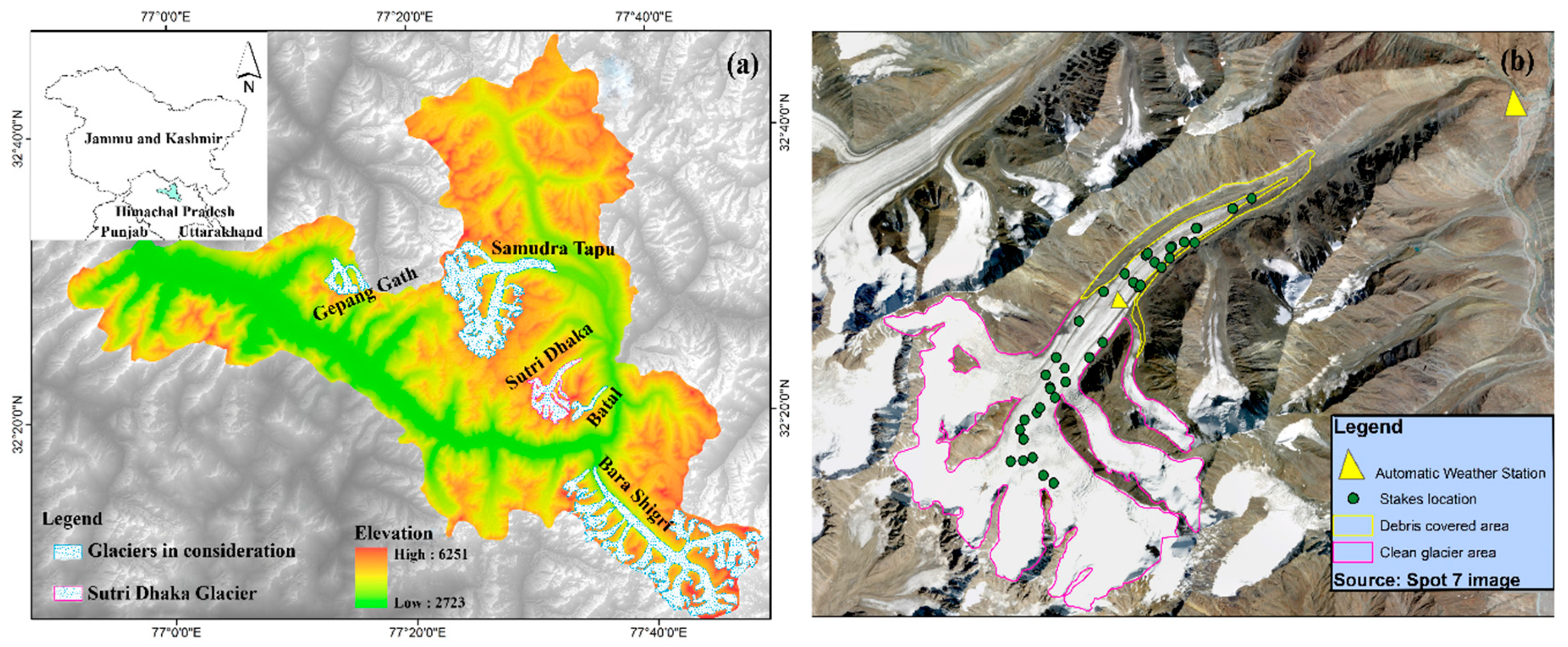
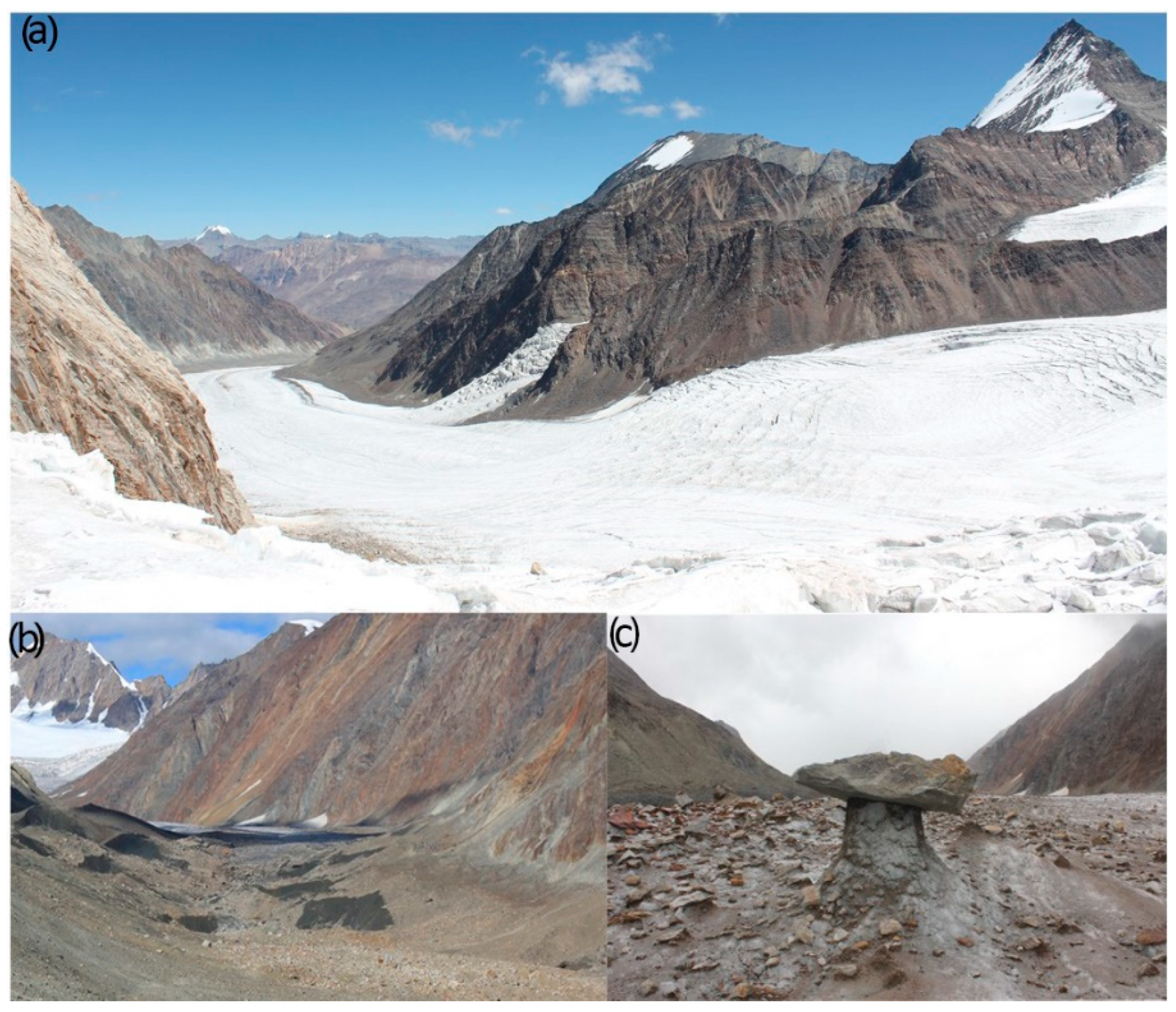
2.1. Study Area

The study area lies in the Chandra Basin, western Himalaya, which falls in a semi-arid zone that contains ~201 glaciers, of which five have an area >20 km². Hence, glaciers in this region are more sensitive to climate variations, owing to the precipitation pattern influenced by the intensity of monsoon and western disturbances (WD) [39,40,41,42]. The Sutri Dhaka Glacier is a compound valley-type glacier that was formed by four cirques having a length of ~11 km with an elevation range between 6000 m at the head and 4500 m at the snout [42]. The glacier has an east facing orientation with an eastward cirque aspect of gentle slopes (Figure 1).

The lowermost area (4500–4600 m asl) of the glacier is covered with debris of varying thickness (Figure 2b). The ablation zone extends between 4500 and 4900 m and it has many features that are associated with the extensive ice melt, such as glacier tables (Figure 2c) and supra-glacial meltwater channels.

The basin is characterized with widespread debris-covered glaciers to clean ice glaciers (e.g., Bara Shigri ~110.7 km², Samudra Tapu ~79 km² and Sutri Dhaka ~19.6 km²) [23,41,43]. The melt water stream that emerges from the Samudra Tapu Glacier is the main source of the Chandra River, which flows South and then turns northwest near Bara Shigri Glacier (Figure 1). The valley orientation divides the Pir-Panjal range and the Greater Himalayan range with the monsoonal and arid influenced zones [44]. The Chandra Basin is characterized as cold desert with a very short growing season and sparse vegetation due to its position in the rain shadow on the leeward side of the mountains.

Domesticated herds migrate to the Sutri Dhaka catchment every year in summer (June to September) to the elevations of 4500 m and above snow and glacier melt are the main sources of water.

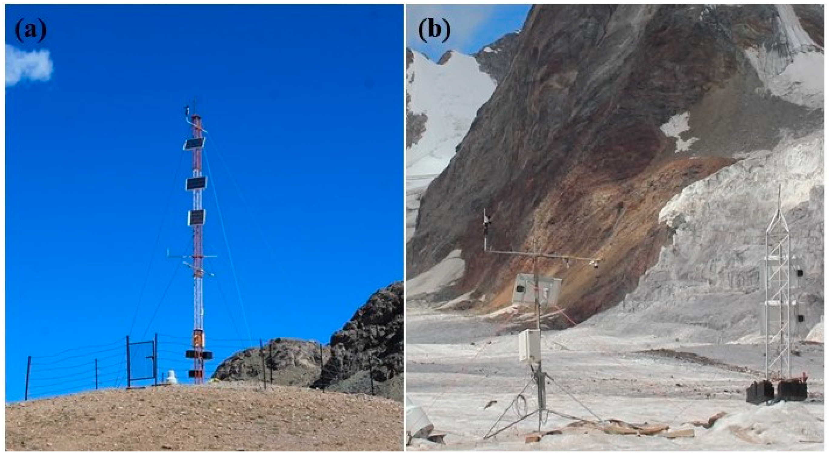
2.2. Installation of AWS and Data Collection

Selected glacier catchments in the Chandra Basin have been systematically monitored for multidisciplinary research programmes under the project entitled “Cryosphere and Climate” by National Centre for Polar and Ocean Research (NCPOR) since 2013. A total of five glaciers (Samundra Tapu, Sutri Dhaka, Batal, Bara Shigri, and Gepang Gath) were selected for studying various glaciological aspects, such as mass balance, snow and glacier hydrology, high-altitude meteorology, meltwater chemistry, geospatial, and glacier dynamics. In the Sutri Dhaka Glacier catchment, two Campbell Scientific AWSs has been operational since the end of September 2015. The deployment of AWSs in high-altitude terrain has increased the accuracy of the meteorological observations and the visualization of measured parameters. These observations provide automatic data collection, processing, and transforming these signals to the data logger. Details of locations with surrounding characteristics of the AWSs installed in the Sutri Dhaka catchment are as follows:

(i)

AWS at Himansh base camp (Hbc, 4052 m asl) is located in an open ground with a gentle slope having a NE aspect. It lies below ~3.5 km (aerial distance) from the present snout at 4500 m asl of the Sutri Dhaka Glacier (Figure 1b and Figure 3a).

(ii)

AWS at Advance base camp (Abc, 4864 m asl) is situated on the clean ice of Sutri Dhaka Glacier. The katabatic wind highly affects this location. The area around this AWS is characterized by year-round snow/ice surface (Figure 1b and Figure 3b).

The temperature probe (HC2S3) was mounted on a metal pole at ~2 m above the surface on both the AWSs to acquire the air temperature data. The probe with a measurement range from −40 °C to +60 °C with an accuracy of ±0.1 °C was naturally housed inside a ventilated radiation shield. This sensor measures the air temperature in five seconds interval, which is automatically averaged for 10 and 30 min while using AWS programming software and is stored in a Campbell Scientific CR1000 data logger. In this study, we calculated the daily minimum (tmin), maximum (tmax), and average temperature (tavg) while using 30 min interval data. Data quality was tested as a range and spatial consistency associated to date and time [45].

2.3. Data Analysis

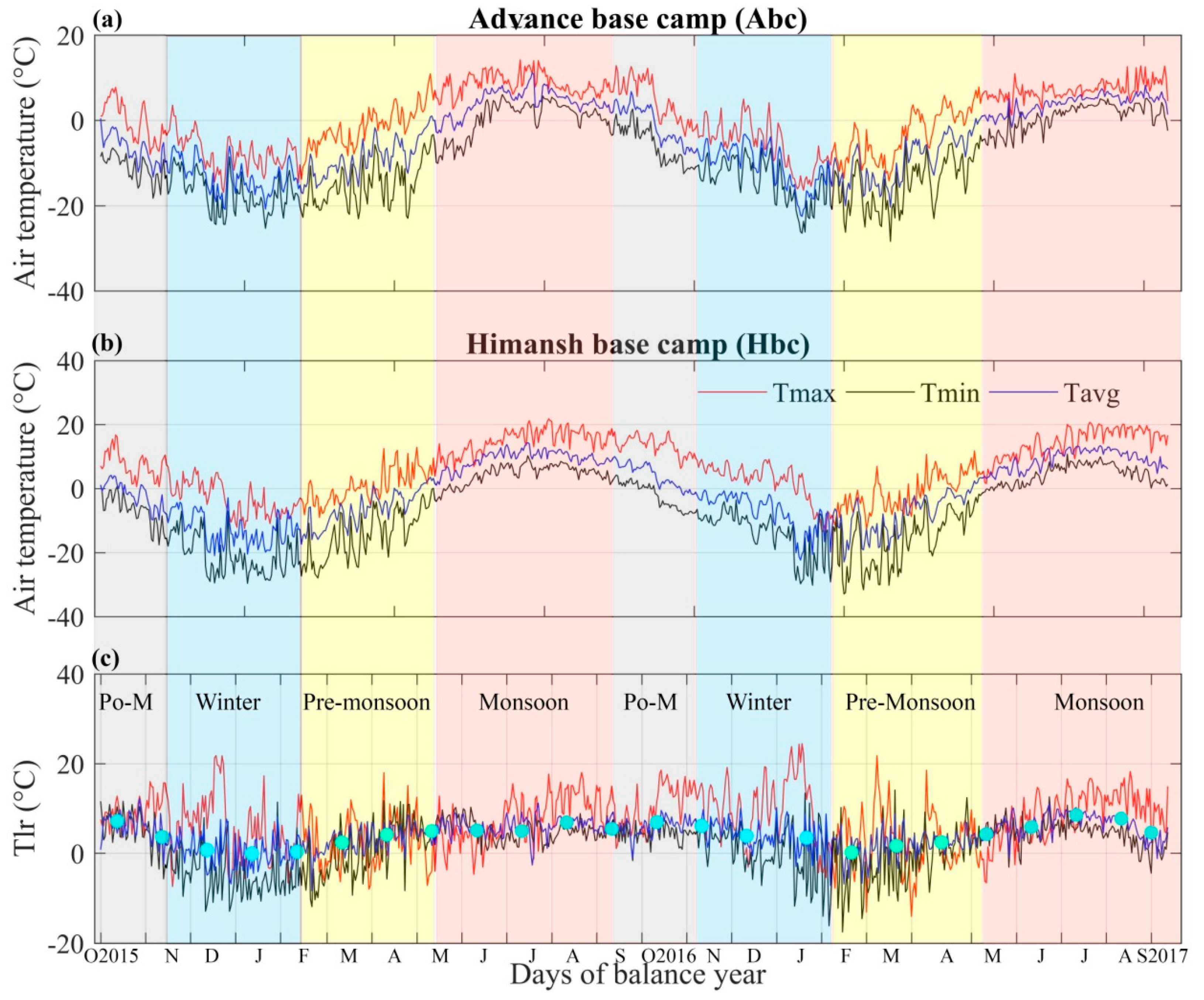
2.3.1. Analysis of Air Temperature Lapse Rate (tlr)

The decrease in air temperature with altitude that was observed by the shielded temperature sensor at 2 m height is known as the temperature lapse rate (tlr) [33,46].

tlr between two stations were obtained while using the following equation:

$$\mathrm{tlr}=\frac{\mathit{dt}}{\mathit{dZ}}=\frac{{\mathrm{t}}_1-{\mathrm{t}}_2}{{\mathrm{Z}}_2-{\mathrm{Z}}_1}$$

(1)

where, t₁ and t₂ are the air temperatures (°C) of the two stations (Hbc and Abc) and, Z₁ and Z₂ are their respective elevation in m asl [46,47]. Here, we have used positive tlr. A higher positive value represents steeper dt/dZ (i.e., large decrease in temperature with elevation) and a relatively less positive value corresponds to shallower dt/dZ [48].

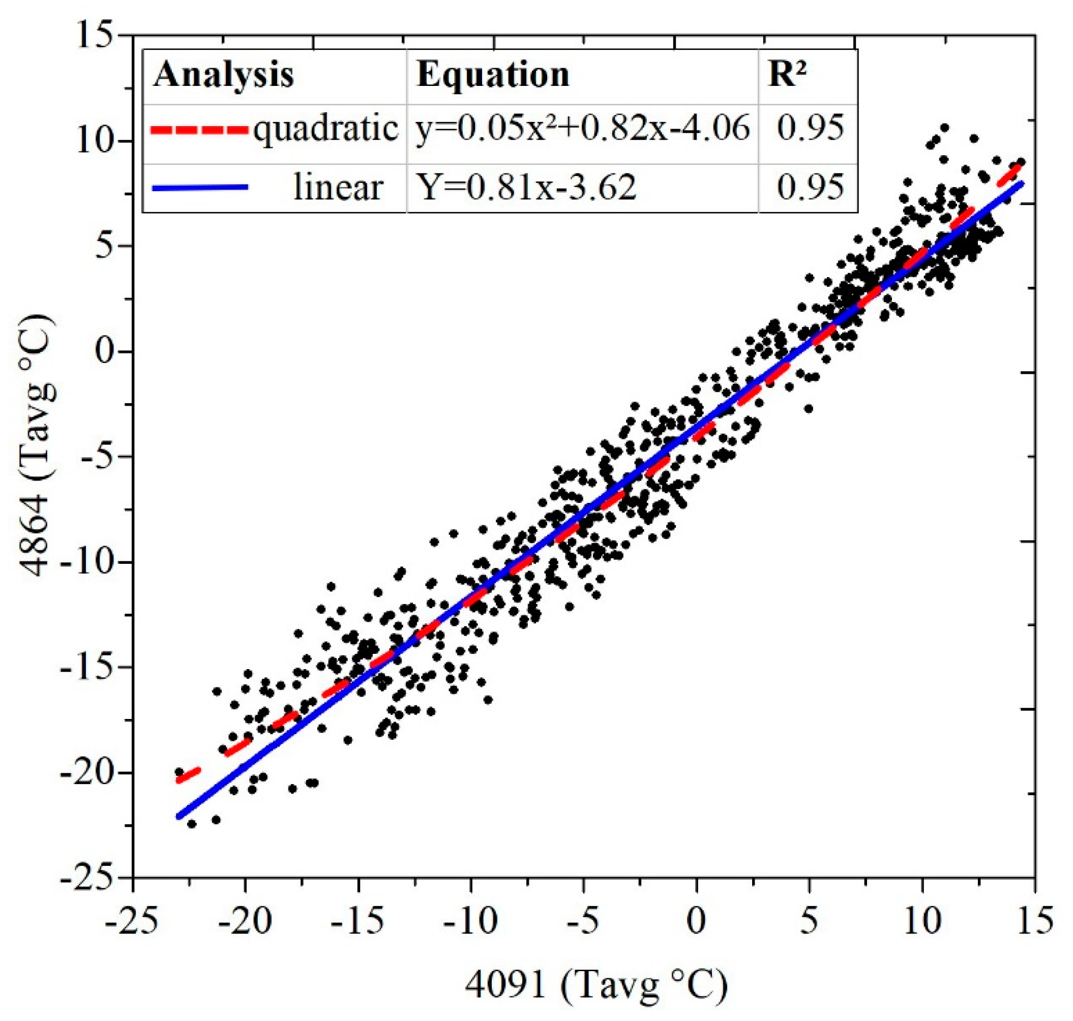
2.3.2. Extrapolation of Average Air Temperature

The tlr facilitates the interpolation and extrapolation of air temperature from stations to locations at a different elevation. This method has been commonly used in many distributed glacier surface melt models that often forced using air temperature that was extrapolated from the station measurements using temperature lapse rate [22,49,50].

We used a linear regression model that extrapolated daily average temperature (t_avg) data at each 100 m elevation using daily tlr between the Hbc and Abc to examine the temperature-elevation relationship, as following:

t₁₀₀ = t_L + (tlr) × A

(2)

where t₁₀₀ is the temperature (in °C) at the increased 100 m elevation. t_L: temperature (in °C) at the lower station. A: altitude can be changed to extrapolate at any elevation accordingly

The extrapolation is based on daily temperature data showing a temperature–elevation relationship for the balance year from 1 October 2015 to 30 September 2017 (two balance years).

Zero degree isotherm (Z_{t = 0}) is a height where the temperature is found to be nearly zero (0 °C) and it is generally used to evaluate the phase change (rain or snow) over the glacier surface. The above extrapolation is carried out up to 5600 m asl to show the range of 0 °C isotherm. Furthermore, a heat map was prepared to understand the time period of melting or freezing condition of a glacier surface in a particular balance year. Therefore, the shifting of temperature isotherms mainly Z_{t = 0} defines the warming on the glacier surface.

2.4. Measurement of Glacier Surface Ablation

The surface ablation of Sutri Dhaka Glacier was estimated by installing a network of 25–30 stakes, where 2–3 stakes were installed in the debris-covered area at the end of the ablation period during 2015–2016 and 2016–2017, which was in compliance with the established methodology and terminology given by [51,52] (Figure 1). These stakes were installed based on the area and surface condition. A dense network was installed in the lower ablation zone, owing to its discrete surface conditions, while the frequencies were reduced in the upper ablation region [53]. For the surface melting, we estimated the heights of each stake exposed with time and then multiplied the measured stake-height differences by the measured 1m surface ice density (i.e., 0.87 gm/cm³, field observation in 2016). Each stake was measured on a monthly basis throughout the summer period for estimating the summer ablation, whereas, the winter ablation was calculated from the cumulative melt from October to June. The annual ablation is calculated by adding the winter and summer ablation. An overall uncertainty of ~20% was considered while considering the measurement errors, the tilting of stakes, and the emergence of stakes due to filling of water in the hole during summer [52].

2.5. Temperature-Index Model for Ice Melt

The summer ice melt is computed while using the temperature-index model (T-index model), providing in-situ temperature data [22,54,55] and validated with the measured surface ablation. The model computes the depth of ice ablation in relation to positive air temperature measured at 2 m height above surface. The sum of all the cumulative positive degree days (CPDD) were multiplied with the degree day factor of ice and debris (DDF, mm C⁻¹ day⁻¹) to get ice melt in water equivalent. The model is described by the following equation:

$$M=\{\begin{array}{cc}DDFice,debris\left(ta-tm\right);& ifta>tm\\ \hfill 0;& ifta<tm\end{array}$$

(3)

where M is the daily melt, DDFice/debris denotes the degree-day factor of ice/debris (mm d⁻¹ °C⁻¹), ta is the average daily temperature, and tm the threshold temperature (usually, 0 °C) for melt. ta > tm tends to produce ice melt, subsequently ta < tm means no melting.

The value of DDF for ice varies with regions in Indian Himalaya, given 7.4 mm for Dokriani Glacier, central Himalaya [55] and 8.32 mm d⁻¹ °C⁻¹ for Chhota Shigri Glacier, western Himalaya [22]. For the present study, we constructed DDF for ice of 8.91 mm d⁻¹ °C⁻¹ while using four points measurement between 4800 and 4900 m asl for different time period in summer and performed against the PDD observed at 4864 m asl. DDF debris 6.54 mm d⁻¹ °C⁻¹ for debris-covered area was obtained from single stake measurements between 4500 and 4600 m asl.

The ice ablation starts in May and extended up to 4800 m asl by June, as observed through in-situ measurements. In this case, DDF for snow was not considered, as the snow surface melts by the end of June. The model has been run from 1 June to 30 September to calculate ablation while using daily extrapolated air temperature (daily PDD) for every 100 m elevation range.

The debris-covered area is mostly constrained in elevation range of 4500–4600 m, including clean ice area in the centre. Additionally, narrow parts of the glacier margin are debris-covered, but no stakes were installed due to high rock fall from the mountain wall (Figure 1). Therefore, model for debris area was only performed between 4500 and 4600 m asl.

3. Results and Discussion

3.1. Air Temperature and Temperature Lapse Rate (tlr)

Air temperature is an important meteorological parameter that is required to estimate snow and ice ablation, which is a period of positive temperature and melt runoff of the glacierized area [56,57]. The daily air temperature variabilities at both sites (Hbc-Abc) are almost similar in winter and pre-monsoon, with large differences in the monsoon and post-monsoon season indicating strong inter-seasonal variability (Figure 4a,b). The daily minimum and maximum temperatures were the highest in July, followed by August with the positive temperature at both sites (Figure 4a,b). The variation in the minimum and maximum temperature ranges between 5–10 °C, which reflects the effects on weather condition in semi-arid region. The higher difference in tavg during the summer months to the winter months indicate warming of the lower altitude, the melting of snow surface, and lower albedo results in more absorption of solar heat. While, the western disturbances (WDs) often bring cold air parcels causing a reduction in temperature over a large part of the Himalayan region in the winter months. Moreover, the sharp decrease in tavg during post-monsoon indicates the onset of the winter season or the effects of the prevailing westerlies bringing cold air masses (Figure 4a). As summer precipitation is scarce in the region, it has less impact on the diurnal temperature (Figure 4a). Very few events were observed in the down station (Hbc) in the form of drizzle (i.e., five events during August–September 2017; total cumulative rain of ~32.8 mm, ranging from 1.7 to 17.2 mm).

During the monsoon season, variations in daily and monthly temperatures are crucial for an understanding of spatial distribution of snow cover and its melt in the catchment. In 2016 and 2017, the mean temperature for the summer period (JJAS) was found to be 9.6 °C and 9.2 °C at Hbc (4052 m asl) and 3.7 °C and 5.0 °C at Abc (4864 m asl), respectively. In summer, temperature gradient intensifies the prevailing valley wind which results in high temperatures causing extreme melting condition in the Sutri Dhaka catchment. The maximum air temperature (11.4 °C and 7.4 °C) was found in July, and the minimum (−15 °C and −15.7 °C) in January at both sites, showing a similar weather trend in the catchment. These results have similar temperature trends (maximum in July and minimum in January) that were observed in the nearby Chhota Shigri Glacier, western Himalaya [58] and Dokriani, Chorabari, and Dunagiri glaciers in central Himalaya [56,59].

The daily tlr has shown considerable fluctuation in different months, as well as seasonal and interannual variation. Overall, the tlr for the balance years of 2015–2016 and 2016–2017 was lowest 0.35 and 2.5 °C km⁻¹ in the months of DJF (winter) and highest 5.6 °C and 6.8 °C km⁻¹ in JJAS (Monsoon) (Figure 4c). The high variability in the daily cycle of tlr (minimum, maximum and average) is found in the winter season and during pre-monsoon months when inversion are common. Under these conditions, the effect of katabatic wind blowing down the slope causes temperature inversion. Whereas, the monsoon period with a comparatively high tlr of 5.6–6.8 °C km⁻¹ shows large temperature differences between two observational sites. These observations do not agree to the study that was reported by [60] in Langtang River catchment in Nepal Himalaya and in Dokriani Glacier, Garhwal Himalaya [29], which showed lowest tlr during the monsoon period, owing to the moisture influx in the region. Even though the largest tlr were observed in summer and the lowest in in winter, which is contrary to other studies, the summer tlr was in the range of (~6–7 °C km⁻¹ as in other high-altitude Himalayan regions. Several records that represents the steep monsoon lapse rate and the shallow lapse rate of the other seasons in the western Himalaya were investigated (

Table 1. Seasonal and annual tlr calculated using daily temperature dataset for different glacierized catchments of the western Himalaya with statistical analysis of standard deviation for the Sutri Dhaka Glacier Catchment.

Region	Glacier Catchment	Elevation Range (m asl)	Year	Near-Surface (Slope) Lapse Rate °C km−1					References
				December, January, February	March, April, May	June, July, August, September	October, November
				Winter	Pre-Monsoon	Monsoon	Post-Monsoon	Annual
Chandra Basin, LahaulSpiti	Hamtah Glacier	3330–3940	2002–2006	-	-	11.4	-	-	[36]
Chandra River, Himachal Himalaya	Chhota Shigri, Lahaul-Spiti			-	-	-	-	3.8–6.7	[61]
		1092–4863	2009–2012			-	-	6.4	[22]
Gilgit-Baltistan, Karakoram Himalaya	Baltoro Glacier	3048–4050	2003	6.9	7.7	7.2	8.8	7.5	[62]
Chandra Basin	Sutri Dhaka Glacier	4052–4864	2015–16 2016–17	0.35 ± 0.3 2.5 ± 1.9	3.8 ± 1.2 2.8 ± 1.3	5.6 ± 0.8 6.8 ± 0.1	6.5 ± 0.1	4.2 ± 2.4 4.6 ± 2.5	Present study

).

The annual (October to September, a balance year) tlr between Hbc and Abc was found to be 4.2 °C km⁻¹. This range of lapse rate was significantly different from other basins of the Himalaya, which demonstrated the need to use localized tlr instead of the uniform environmental lapse rate (i.e., 6.5 °C km⁻¹) in the region (Table 1; [29]). The tlr in the monsoon season approximately equals to the environmental lapse rate (6.5 °C km⁻¹) (Figure 4b). Furthermore, we have observed limited variability and smooth mean monthly monsoon and post-monsoon seasonal tlr ranging between 5.6–6.8 °C km⁻¹ supported by the lowest standard deviation.

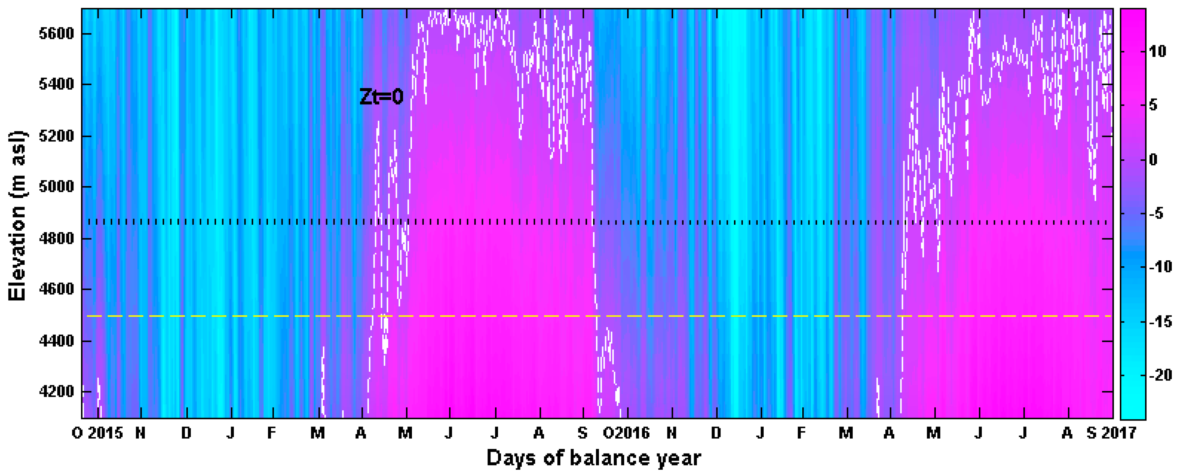
3.2. Spatial Distribution of Air Temperature

The spatial distribution of air temperature in the upper reaches of the Himalaya has greater value for defining the potential phase change of rain and snow and melt period, which generally tends to occur above °C isotherms Z_{t = 0} [28,29]. Changes in temperature isotherms as a function of elevation and time can be assessed by extrapolating lower station temperature data based on the observed tlr. As known previously, the temperature gradient shows a decreasing trend, with increasing altitude making up a systematic linear trend and a quadratic fit with altitude [63]. Both linear and second order polynomial fit between the Hbc and Abc had a good agreement with R² = 0.95 for the model’s validation (Figure 5). Therefore, the daily average temperatures that were calculated at two sites (i.e., 4052 and 4864 m asl) were extrapolated between 4052–4864 and 4864–5664 m asl using daily tlr. Although data from only two stations were used, potentially both of the stations are situated in the same glacierized valley (Figure 1).

Our study showed that the temperature gradually increased above freezing points (0.2–1.2 °C) by June, sustaining till the end of the ablation period (i.e., 30 September). The observed tavg of 3.7–5.0 °C at the Abc (4864 m asl) revealed sufficient melting temperature to change ice into water. As the slope of the Sutri Dhaka Glacier is ~20° (ablation zone), as soon the ice turns into water it either percolates or flows over the ice surface distributing its energy into ice during refreezing.

The white dotted line in Figure 6 is the °C isotherm (Z_{t = 0}), which signifies the period of melting under the positive condition for the Sutri Dhaka Glacier. The behavior of Z_{t =0} over the glacier surface concurs with the phase (snow or rain) change, snow line fluctuation, and glacier surface melting condition [64,65,66]. From Figure 6, it is evident that the derived tavg ranged from 14.0 to −24.0 °C between the elevation of 4052 and 5664 m asl. Based on the extrapolated average temperature (tavg), the highest Z_{t = 0} was found between 5200 and 5500 m asl, until it declined at the end of the ablation period. The Z_{t = 0} sharply reacts to its maximum elevation (5500 m asl) in June and it remained there for the whole summer period. This suggests that the higher positive sensible and latent heat flux over the ablation zone of the glacier surface tend to enhance the ice ablation. The maximum range of Z_{t = 0} was found to overlap with the equilibrium line altitude (ELA, average ~5365 m asl) that was observed at the end of ablation period through mass balance observation during 2015–17 (

Table 2. Observed surface ablation of the Sutri Dhaka Glacier during 2015–16 and 2016–17.

Year/Period of Measurements	No of Stakes	Winter Ablation (m w.e.)	Summer Ablation (m w.e.)	Annual Ablation (m w.e.)	ELA (m asl)
2015–16 Winter: 1. 1 October 2015 to 16 June 2016. Summer: 2. 16 to 30 June 2016. 3. 1 to 3 July 2016. 4. 1 to 31 August 2016. 5. 1 September to 2 October 2016.	24	−0.46 ± 0.09	−3.74 ± 0.74	−4.20 ± 0.84	5410
2016–17 Winter: 1. 3 October 2016 to 25 June 2017. Summer: 2. 26 June to 31 July 2017. 3. 1 to 31 August 2017. 4. 1 to 15 September 2017. 5. 16 to 30 September 2017	28	−0.38 ± 0.07	−2.71 ± 0.54	−3.09 ± 0.62	5320

). Therefore, the estimation of Z_{t = 0} over the glacier surface can be used as a marker of ELA in the absence of in-situ observations.

The observed Z_{t = 0} sharply declined (negative) in the first week of October, which was probably because of the offset of monsoon and the onset of western disturbances. These results are similar to the air temperature that was observed over the Chhota Shigri Glacier in Chandra basin, which showed a sudden drop that was characterized by the change of summer monsoon to post-monsoon, followed by winter seasons [67]. This phenomenon was also observed in Bhagirathi basin, central Himalaya, concluding the short-lived transition phase between monsoon and post-monsoon season [29,66]. Unlike the sudden drop in Z_{t = 0} during the summer period of 2017, we did not find any daily variation in the summer of 2016 (Figure 6). Previously, [67] have clearly correlated the sudden drop in the air temperature during summer with rainfall and snowfall events. The highest elevation of Z_{t = 0}, ~5600 m was also found in 2016 when compared to 2017 summer. The higher and sustained Z_{t = 0} in 2016 revealed higher melting days and probably high surface melt (Table 2).

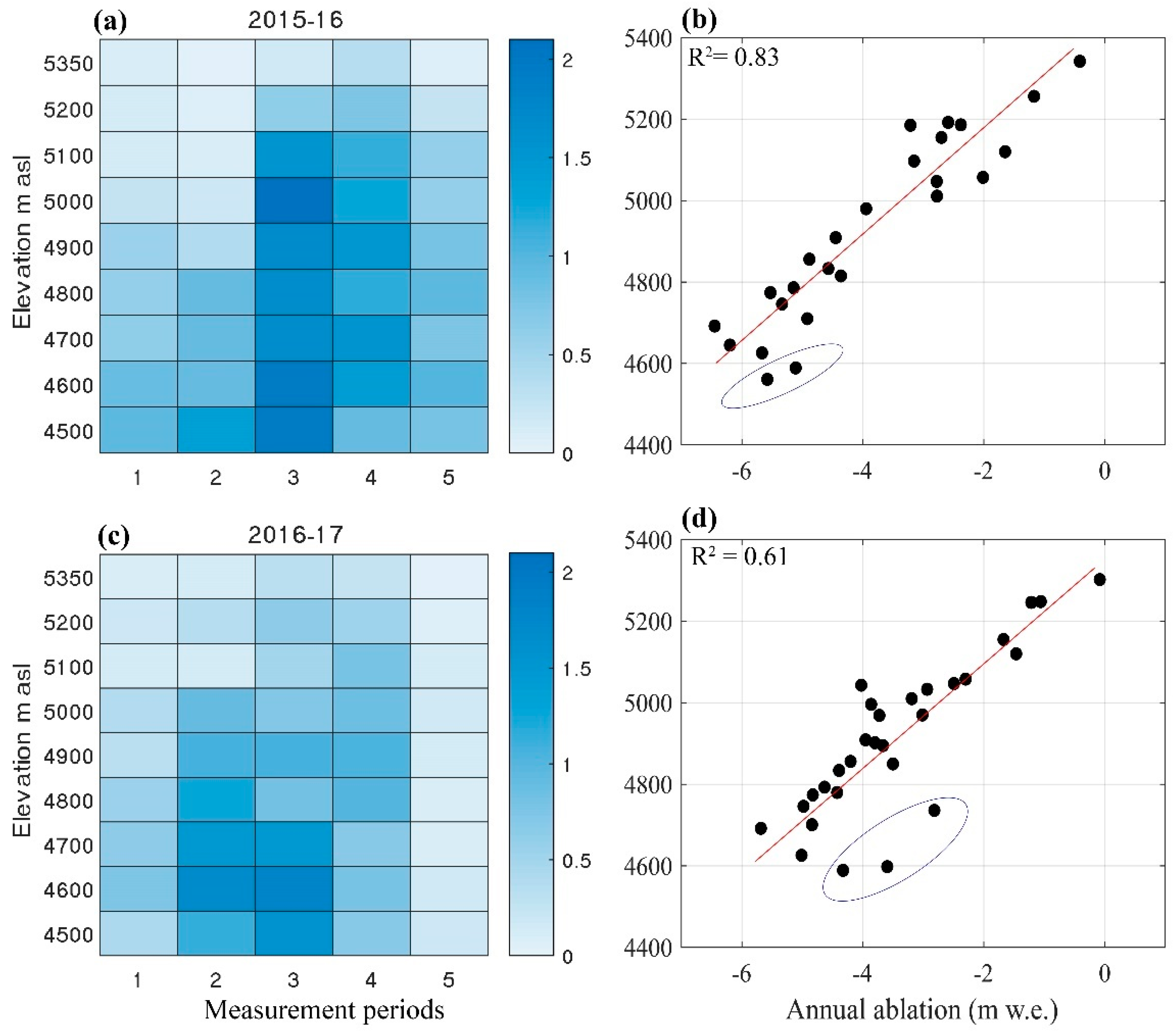
3.3. Seasonal Variability in Surface Melting

The field and remote sensing data suggests that ~14% of Sutri Dhaka Glacier’s ablation zone is under debris cover [42]. This classifies Sutri Dhaka as a clean ice type (C-type) glacier exposing higher ablation area (Figure 2a). In compliance with this, several studies have reported the increase in debris-covered area with the retardation in ablation underneath and a lower recession rate, however higher melting rate on the wide and clean ice ablation area [68,69,70]. The observed winter ablation and the monthly summer ablation reflect the distinct temporal and spatial pattern in the melting magnitude (Figure 7a,c). During three seasons i.e., pre-monsoon, winter, and post-monsoon of 2015–16 and 2016–17, the glacier had a cumulative melting of −0.46 and −0.38 m w.e. between 4500 and 5350. Reduced melt is related to the cold westerly advection and winter snow accumulation [71].

Snow depth measurements between 4700 and 5200 m asl that were conducted in May show that 1.4–1.6 m of snow was accumulated. A recent study by [72] has also observed a similar average accumulated SWE of 0.624 m and 0.496 m during March of 2009 and 2010 over the Samudra Tapu Glacier. Therefore, the ice melt in three seasons suggests the role of snow cover and temperature gradient between the elevations, where the ice surface at lower elevation gets exposed early when compared to that of snow-covered higher elevation. A study in the Zanskar range, western Himalaya for snow cover assessment showed that the snow melt starts in March and it continues until June extending to 4500–4800 m [71,73]. Therefore, as a consequence of snow cover over the glacier, the ice ablation starts in May, which has been observed during the early days of June on Sutri Dhaka Glacier when stakes between 4500 and 4900 indicate ice ablation (Figure 7a,c). Positive air temperatures, as recorded by AWS, show that ice melt can continue into October (Figure 4a).

During the summer, the ice ablation gradually increased to its maximum in the month of July and August (Figure 7a,c). The higher ablation rate in summer is well correlated with the rise in temperature tavg in the catchment. This period is also known as the peak summer melting season throughout the Indian Himalaya. The cumulative ablation during summer period between 4500 and 5350 m asl was found to be −3.74 ± 0.74 and −2.71 ± 0.54 m w.e. for 2016 and 2017, respectively. The ablation was found to be maximum ~88% of total ice melt during summer (four months, JJAS) in comparison to the reduced melting of ~12% during three seasons (eight months).

Figure 7b,d shows how annual ablation changes with the altitude (known as ablation gradient). The annual ablation gradient for clean ice was linear (R² = 0.83), showing a systematic decline of melting magnitude with the elevation similar to tavg. The annual ablation rate at the interval of 300 m asl above the snout (i.e., 4500–4800 m) ranged from −4.0 ± 0.8 to −6.5 ± 1.3 m w.e. for both of the balance years. The vertical and cross-sectional (i.e., left to right) ablation gradient shows the importance of a number of point measurements with different elevation and surface conditions. Substantial ice ablation now progressively exposes the debris along the side margins of the glacier and forms the ice wall and supra-glacial channels in the lower ablation zone (Figure 2b,c; Table 2).

A comparison of our results with the ablation gradient on the Chhota Shigri Glacier in Chandra basin showed that both of the glaciers had a similar ablation rate (−6.0 to −2.0 m w.e.) within the same altitudinal range (i.e., 4500 to 5000 m asl) [74], whereas Dokriani Glacier showed a similar ablation rate of −5.5 to −2 m w.e. only in the lower elevation zone of 4100–4400 m asl in the central Himalaya [70]. From these observations, we demonstrate that, although the glaciers of western Himalaya occupy at higher altitudes, they have higher melting rates when compared to the narrow central Himalayan glaciers in the lower altitude. Such findings indicate the change in mass balance gradient that shifts up and down and can be considered to be independent to altitude on different climatic states [75].

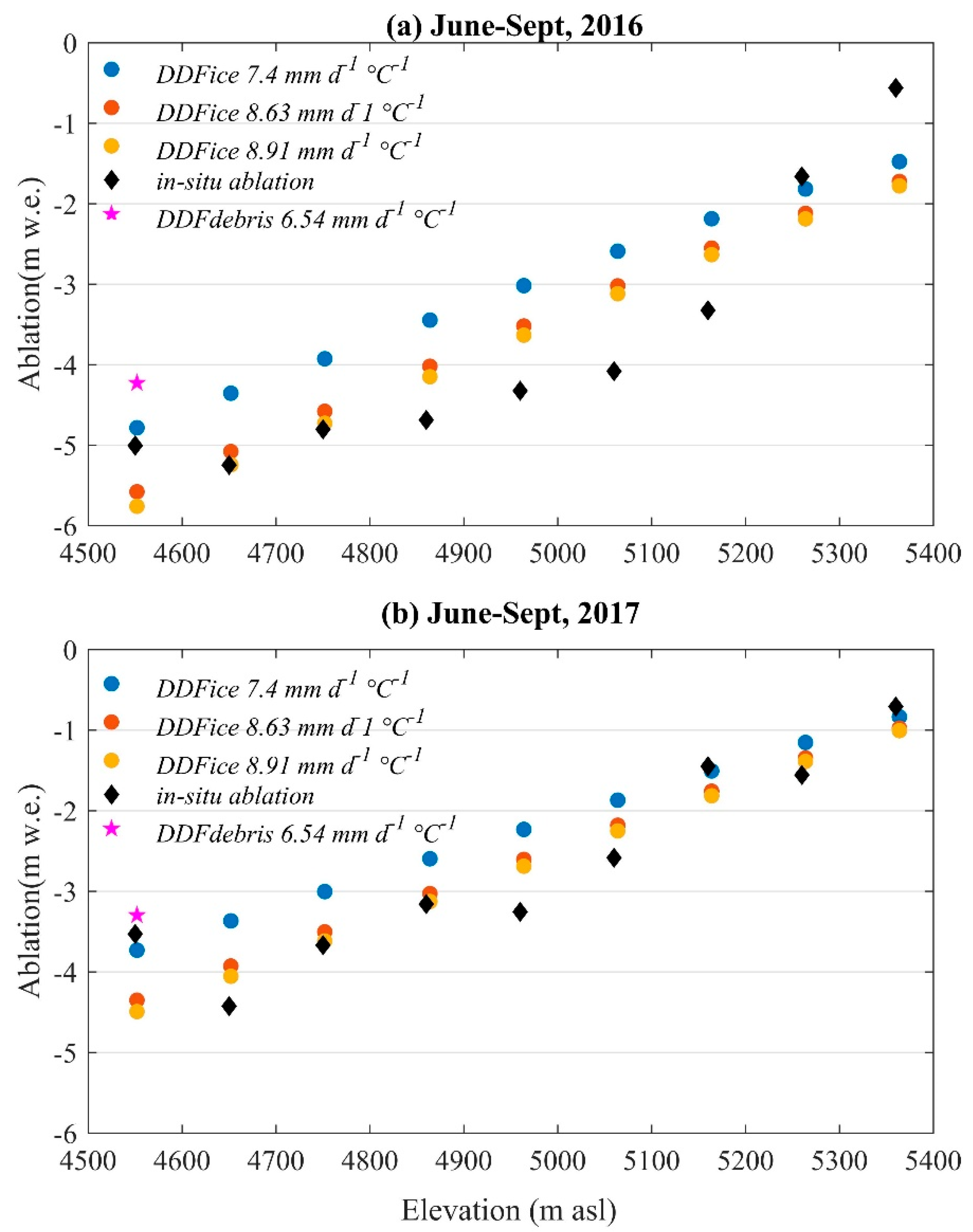
3.4. Evaluation of Modeled and Observed Melting

An empirical relationship for ice melt (T-index model) is analyzed for the period from June to September (2016 and 2017) to standardize the observed melting and effects of air temperature. In-situ and remote sensing survey for supraglacial debris thickness and coverage measurement indicated that the maximum debris cover was limited to ablation zone between 4500 and 4600 m asl (Figure 1b). The melt factors calculated for Sutri Dhaka Glacier and the derived results modestly vary with the observed melting. The melting as a function of CPDD shows a linear decrease with elevation, whereas in lower reaches (4500–4600 m), debris plays a role in the reduction of ice melting underneath (Figure 8a,b).

The difference in modeled ablation based on DDF debris and in-situ debris ablation varies between 16% and 7% during 2016 and 2017, respectively (Figure 8a,b). However, the modeled ablation for the debris covered area when computed using DDFice varies between 14% and 23% to the in-situ debris ablation. When comparing the relative difference between clean ice melt (4600–4700 m asl) to the debris cover ice melt (4500–4600 m asl), the values vary from 6% to 27%. This is related to the insulation effects of debris thickness and distribution in the lower part of Sutri Dhaka Glacier. These findings are comparable to the results from other studies on Himalayan glaciers that found good relation between T-index simulated and measured melting [22,59,70]. It is obvious from the results that temperature is the dominant factor for ice melting, even for the debris-covered areas.

4. Conclusions

It is well known that glaciers melt water regulates the water availability in the downstream with a suitable dimension providing possibilities for hydropower generation. We have conceptualized the air temperature and glacier surface melting and highlight the higher melting rate during a very short summer (JJAS) in the monsoon-arid zone of western Himalaya. The tlr for the balance year 2015–16 and 2016–17 shows lowest <2 °C km⁻¹ in the winter and highest 5.7 and 6.6 °C km⁻¹ in post-monsoon and monsoon season. The annual tlr, including all season (winter, pre-monsoon, monsoon, and post-monsoon) was found to be 4.2 °C km⁻¹. This reemphasizes the significance of using a catchment level determined lapse rate in place of a regional/global lapse rate for glacier and hydrological modelling.

A rapid increase in air temperature in June shows the onset of the summer monsoon period and then a sudden drop of temperature in the first week of October suggests the start of post-monsoon (cold and dry) season in the Sutri Dhaka Glacier catchment. In compliance with positive air temperature in JJAS, ablation was also found to be maximum ~88% of total ice melt in the four months and ~12% in the other eight months.

The analysis of °C isotherms shows a sharp incline of Z_{t = 0} that reacted to the maximum elevation (5000–5500 m asl) in June and sustained there for the full summer period. Later, Z_{t = 0} sharply declined in the first week of October, which was probably because of the offset of the monsoon and onset of the western disturbance.

Our study found a high correlation between mean annual ablation and altitude showing a pattern that was similar to the temperature and altitude relationship. The altitudinal T-index modelled and observed melting for June to September 2016 and 2017 are in close agreement, revealing the role of air temperature in glacier surface melting. Further, the detailed investigation of high temporal and spatial resolution relationship between melting and atmospheric enegry fluxes is required for understanding the response of glaciers towards climatic variations.

References

1. Bhambri, R.; Bolch, T.; Kawishwar, P.; Dobhal, D.P.; Srivastava, D.; Pratap, B. Heterogeneity in glacier response in the upper Shyok valley, northeast Karakoram. Cryosphere 2013, 7, 1385–1398. [Google Scholar] [CrossRef] [Green Version]
2. Bolch, T.; Kulkarni, A.; Kaab, A.; Huggel, C.; Paul, F.; Cogley, J.G.; Frey, H.; Kargel, J.S.; Fujita, K.; Scheel, M.; et al. The State and Fate of Himalayan Glaciers. Science 2012, 336, 310–314. [Google Scholar] [CrossRef] [PubMed] [Green Version]
3. Hewitt, K. The Karakoram anomaly? Glacier expansion and the ‘elevation effect,’ Karakoram Himalaya. Mt. Res. Dev. 2005, 25, 332–340. [Google Scholar] [CrossRef]
4. Kaab, A.; Berthier, E.; Nuth, C.; Gardelle, J.; Arnaud, Y. Contrasting patterns of early twenty-first-century glacier mass change in the Himalayas. Nature 2012, 488, 495–498. [Google Scholar] [CrossRef] [PubMed]
5. Singh, P.; Bengtsson, L. Hydrological sensitivity of a large Himalayan basin to climate change. Hydrol. Process. 2004, 18, 2363–2385. [Google Scholar] [CrossRef]
6. Azam, M.F.; Wagnon, P.; Berthier, E.; Vincent, C.; Fujita, K.; Kargel, J.S. Review of the status and mass changes of Himalayan-Karakoram glaciers. J. Glaciol. 2018, 64, 61–74. [Google Scholar] [CrossRef] [Green Version]
7. Fujita, K.; Nuimura, T. Spatially heterogeneous wastage of Himalayan glaciers. Proc. Natl. Acad. Sci. USA 2011, 108, 14011–14014. [Google Scholar] [CrossRef] [Green Version]
8. Pratap, B.; Dobhal, D.P.; Bhambri, R.; Mehta, M.; Tewari, V.C. Four decades of glacier mass balance observations in the Indian Himalaya. Reg. Environ. Chang. 2016, 16, 643–658. [Google Scholar] [CrossRef]
9. Vincent, C.; Ramanathan, A.; Wagnon, P.; Dobhal, D.P.; Linda, A.; Berthier, E.; Sharma, P.; Arnaud, Y.; Azam, M.F.; Jose, P.G.; et al. Balanced conditions or slight mass gain of glaciers in the Lahaul and Spiti region (northern India, Himalaya) during the nineties preceded recent mass loss. Cryosphere 2013, 7, 569–582. [Google Scholar] [CrossRef] [Green Version]
10. Muhammad, S.; Tian, L.; Nüsser, M. No significant mass loss in the glaciers of Astore Basin (North-Western Himalaya), between 1999 and 2016. J. Glaciol. 2019, 65, 270–278. [Google Scholar] [CrossRef] [Green Version]
11. Bhambri, R.; Bolch, T. Glacier mapping: A review with special reference to the Indian Himalayas. Prog. Phys. Geogr. 2009, 33, 672–704. [Google Scholar] [CrossRef]
12. Garg, P.K.; Shukla, A.; Jasrotia, A.S. Influence of topography on glacier changes in the central Himalaya, India. Glob. Planet. Chang. 2017, 155, 196–212. [Google Scholar] [CrossRef]
13. Kulkarni, A.V.; Bahuguna, I.M.; Rathore, B.P.; Singh, S.K.; Randhawa, S.S.; Sood, R.K.; Dhar, S. Glacial retreat in Himalaya using Indian Remote Sensing satellite data. Curr. Sci. 2007, 92, 69–74. [Google Scholar]
14. Mir, R.A.; Jain, S.K.; Lohani, A.K.; Saraf, A.K. Glacier recession and glacial lake outburst flood studies in Zanskar basin, western Himalaya. J. Hydrol. 2018, 564, 376–396. [Google Scholar] [CrossRef]
15. Immerzeel, W.W.; van Beek, L.P.H.; Bierkens, M.F.P. Climate Change Will Affect the Asian Water Towers. Science 2010, 328, 1382–1385. [Google Scholar] [CrossRef] [PubMed]
16. Nye, J. The mechanics of glacier flow. J. Glaciol. 1952, 2, 82–93. [Google Scholar] [CrossRef]
17. Bhushan, S.; Syed, T.H.; Arendt, A.A.; Kulkarni, A.V.; Sinha, D. Assessing controls on mass budget and surface velocity variations of glaciers in Western Himalaya. Sci. Rep. 2018, 8, 8885. [Google Scholar] [CrossRef] [PubMed]
18. Cogley, J.G. Present and future states of Himalaya and Karakoram glaciers. Ann. Glaciol. 2011, 52, 69–73. [Google Scholar] [CrossRef] [Green Version]
19. Meier, M.F.; Dyurgerov, M.B.; Rick, U.K.; O’Neel, S.; Pfeffer, W.T.; Anderson, R.S.; Anderson, S.P.; Glazovsky, A.F. Glaciers dominate Eustatic sea-level rise in the 21st century. Science 2007, 317, 1064–1067. [Google Scholar] [CrossRef]
20. Acharya, A.; Kayastha, R.B. Mass and Energy Balance Estimation of Yala Glacier (2011–2017), Langtang Valley, Nepal. Water 2018, 11, 6. [Google Scholar] [CrossRef]
21. Kumar, A.; Verma, A.; Gokhale, A.A.; Bhambri, R.; Misra, A.; Sundriyal, S.; Dobhal, D.P.; Kishore, N. Hydrometeorological assessments and suspended sediment delivery from a central Himalayan glacier in the upper Ganga basin. Int. J. Sediment Res. 2018, 33, 493–509. [Google Scholar] [CrossRef]
22. Azam, M.F.; Wagnon, P.; Vincent, C.; Ramanathan, A.; Linda, A.; Singh, V.B. Reconstruction of the annual mass balance of Chhota Shigri glacier, Western Himalaya, India, since 1969. Ann. Glaciol. 2014, 55, 69–80. [Google Scholar] [CrossRef] [Green Version]
23. Tawde, S.A.; Kulkarni, A.V.; Bala, G. An estimate of glacier mass balance for the Chandra basin, western Himalaya, for the period 1984-2012. Ann. Glaciol. 2017, 58, 99–109. [Google Scholar] [CrossRef]
24. Bhutiyani, M.R. Mass-balance studies on Siachen Glacier in the Nubra valley, Karakoram Himalaya, India. J. Glaciol. 1999, 45, 112–118. [Google Scholar] [CrossRef]
25. Bhutiyani, M.R.; Kale, V.S.; Pawar, N.J. Climate change and the precipitation variations in the northwestern Himalaya: 1866-2006. Int. J. Climatol. 2010, 30, 535–548. [Google Scholar] [CrossRef]
26. Shekhar, M.S.; Chand, H.; Kumar, S.; Srinivasan, K.; Ganju, A. Climate-change studies in the western Himalaya. Ann. Glaciol. 2010, 51, 105–112. [Google Scholar] [CrossRef] [Green Version]
27. Azam, M.F.; Wagnon, P.; Vincent, C.; Ramanathan, A.; Favier, V.; Mandal, A.; Pottakkal, J.G. Processes governing the mass balance of Chhota Shigri Glacier (western Himalaya, India) assessed by point-scale surface energy balance measurements. Cryosphere 2014, 8, 2195–2217. [Google Scholar] [CrossRef] [Green Version]
28. Shea, J.M.; Wagnon, P.; Immerzeel, W.W.; Biron, R.; Brun, F.; Pellicciotti, F. A comparative high-altitude meteorological analysis from three catchments in the Nepalese Himalaya. Int. J. Water Resour. Dev. 2015, 31, 174–200. [Google Scholar] [CrossRef] [Green Version]
29. Yadav, J.S.; Pratap, B.; Gupta, A.K.; Dobhal, D.; Yadav, R.; Tiwari, S.K. Spatio-temporal variability of near-surface air temperature in the Dokriani glacier catchment (DGC), central Himalaya. Theor. Appl. Climatol. 2019, 136, 1513–1532. [Google Scholar] [CrossRef]
30. Pradhananga, N.S.; Kayastha, R.B.; Bhattarai, B.C.; Adhikari, T.R.; Pradhan, S.C.; Devkota, L.P.; Shrestha, A.B.; Mool, P.K. Estimation of discharge from Langtang River basin, Rasuwa, Nepal, using a glacio-hydrological model. Ann. Glaciol. 2014, 55, 223–230. [Google Scholar] [CrossRef] [Green Version]
31. Steiner, J.F.; Pellicciotti, F. Variability of air temperature over a debris-covered glacier in the Nepalese Himalaya. Ann. Glaciol. 2016, 57, 295–307. [Google Scholar] [CrossRef] [Green Version]
32. Blandford, T.R.; Humes, K.S.; Harshburger, B.J.; Moore, B.C.; Walden, V.P.; Ye, H.C. Seasonal and synoptic variations in near-surface air temperature lapse rates in a mountainous basin. J. Appl. Meteorol. Climatol. 2008, 47, 249–261. [Google Scholar] [CrossRef]
33. Marshall, S.J.; Sharp, M.J.; Burgess, D.O.; Anslow, F.S. Near-surface-temperature lapse rates on the Prince of Wales Icefield, Ellesmere Island, Canada: Implications for regional downscaling of temperature. Int. J. Climatol. 2007, 27, 385–398. [Google Scholar] [CrossRef]
34. Kattel, D.B.; Yao, T.; Panday, P.K. Near-surface air temperature lapse rate in a humid mountainous terrain on the southern slopes of the eastern Himalayas. Theor. Appl. Climatol. 2018, 132, 1129–1141. [Google Scholar] [CrossRef]
35. Kattel, D.B.; Yao, T.D.; Yang, W.; Gao, Y.; Tian, L.D. Comparison of temperature lapse rates from the northern to the southern slopes of the Himalayas. Int. J. Climatol. 2015, 35, 4431–4443. [Google Scholar] [CrossRef]
36. Siddiqui, M.; Maruthi, K. Detailed glaciological studies on Hamtah Glacier. Lahaul Spiti Dist. HP Geol. Surv. India 2008, 140, 92–93. [Google Scholar]
37. Bookhagen, B.; Burbank, D.W. Topography, relief, and TRMM-derived rainfall variations along the Himalaya. Geophys. Res. Lett. 2006, 33, 5. [Google Scholar] [CrossRef]
38. Thayyen, R.; Gergan, J. Role of glaciers in watershed hydrology: A preliminary study of a “Himalayan catchment”. Cryosphere 2010, 4, 115–128. [Google Scholar] [CrossRef]
39. Krenek, L.; Bhawan, V. Recent and past glaciation of Lahaul. Indian Geogr. J. 1945, 3, 93–102. [Google Scholar]
40. Mayewski, P.A.; Jeschke, P.A. Himalayan and Trans-Himalayan glacier fluctuations since AD 1812. Arct. Alp. Res. 1979, 11, 267–287. [Google Scholar] [CrossRef]
41. Pandey, P.; Venkataraman, G. Changes in the glaciers of ChandraBhaga basin, Himachal Himalaya, India, between 1980 and 2010 measured using remote sensing. Int. J. Remote Sens. 2013, 34, 5584–5597. [Google Scholar] [CrossRef]
42. Sharma, P.; Patel, L.K.; Ravindra, R.; Singh, A.; Mahalinganathan, K.; Thamban, M. Role of debris cover to control specific ablation of adjoining Batal and Sutri Dhaka glaciers in Chandra Basin (Himachal Pradesh) during peak ablation season. J. Earth Syst. Sci. 2016, 125, 459–473. [Google Scholar] [CrossRef] [Green Version]
43. Owen, L.A.; Derbyshire, E.; Richardson, S.; Benn, D.I.; Evans, D.J.A.; Mitchel, W.A. The quaternary glacial history of the Lahul Himalaya, Northern India. J. Quat. Sci. 1996, 11, 25–42. [Google Scholar] [CrossRef]
44. Cordova, M.; Celleri, R.; Shellito, C.J.; Orellana-Alvear, J.; Abril, A.; Carrillo-Rojas, G. Near-surface air temperature lapse rate over complex terrain in the Southern Ecuadorian Andes: Implications for temperature mapping. Arct. Antarct. Alp. Res. 2016, 48, 673–684. [Google Scholar] [CrossRef]
45. Campbell, J.L.; Rustad, L.E.; Porter, J.H.; Taylor, J.R.; Dereszynski, E.W.; Shanley, J.B.; Gries, C.; Henshaw, D.L.; Martin, M.E.; Sheldon, W.M.; et al. Quantity is Nothing without Quality: Automated QA/QC for Streaming Environmental Sensor Data. Bioscience 2013, 63, 574–585. [Google Scholar] [CrossRef] [Green Version]
46. Pepin, N.; Losleben, M. Climate change in the Colorado Rocky Mountains: Free air versus surface temperature trends. Int. J. Climatol. 2002, 22, 311–329. [Google Scholar] [CrossRef]
47. Petersen, L.; Pellicciotti, F.; Juszak, I.; Carenzo, M.; Brock, B. Suitability of a constant air temperature lapse rate over an Alpine glacier: Testing the Greuell and Bohm model as an alternative. Ann. Glaciol. 2013, 54, 120–130. [Google Scholar] [CrossRef]
48. Minder, J.R.; Mote, P.W.; Lundquist, J.D. Surface temperature lapse rates over complex terrain: Lessons from the Cascade Mountains. J. Geophys. Res. Atmos. 2010, 115, 13. [Google Scholar] [CrossRef]
49. Georges, C.; Kaser, G. Ventilated and unventilated air temperature measurements for glacier-climate studies on a tropical high mountain site. J. Geophys. Res. Atmos. 2002, 107, 11. [Google Scholar] [CrossRef]
50. Pellicciotti, F.; Helbing, J.; Rivera, A.; Favier, V.; Corripio, J.; Araos, J.; Sicart, J.E.; Carenzo, M. A study of the energy balance and melt regime on Juncal Norte Glacier, semi-arid Andes of central Chile, using melt models of different complexity. Hydrol. Process. 2008, 22, 3980–3997. [Google Scholar] [CrossRef]
51. Østrem, G.; Stanley, A. Glacier mass-balance measurements: A manual for field and office work; Canadian Department of Energy, Mines and Resources: Ottawa, ON, Canada, 1969; Volume 66. [Google Scholar]
52. Cogley, J.; Hock, R.; Rasmussen, L.; Arendt, A.; Bauder, A.; Braithwaite, R.; Jansson, P.; Kaser, G.; Möller, M.; Nicholson, L. Glossary of Glacier Mass Balance and Related Terms, IHP-VII Technical Documents in Hydrology No. 86, IACS Contribution No. 2; UNESCO-IHP: Paris, France, 2011. [Google Scholar]
53. Fountain, A.G.; Vecchia, A. How many stakes are required to measure the mass balance of a glacier? Geogr. Ann. Ser. A Phys. Geogr. 1999, 81, 563–573. [Google Scholar] [CrossRef]
54. Hock, R. Temperature index melt modelling in mountain areas. J. Hydrol. 2003, 282, 104–115. [Google Scholar] [CrossRef]
55. Singh, P.; Kumar, N.; Arora, M. Degree-day factors for snow and ice for Dokriani Glacier, Garhwal Himalayas. J. Hydrol. 2000, 235, 1–11. [Google Scholar] [CrossRef]
56. Srivastava, D.; Kumar, A.; Verma, A.; Swaroop, S. Analysis of Climate and Melt-runoff in Dunagiri Glacier of Garhwal Himalaya (India). Water Resour. Manag. 2014, 28, 3035–3055. [Google Scholar] [CrossRef]
57. Mukherjee, K.; Bhattacharya, A.; Pieczonka, T.; Ghosh, S.; Bolch, T. Glacier mass budget and climate reanalysis data indicate a climatic shift around 2000 in Lahaul-Spiti, western Himalaya. Clim. Chang. 2018, 148, 219–233. [Google Scholar] [CrossRef]
58. Nijampurkar, V.N.; Bhandari, N.; Borole, D.V.; Bhattacharya, U. Radiometric Chronology of changme-khangpu glacier, sikkim. J. Glaciol. 1985, 31, 28–33. [Google Scholar] [CrossRef]
59. Karakoti, I.; Kesarwani, K.; Mehta, M.; Dobhal, D.P. Extended T-index models for glacier surface melting: A case study from Chorabari Glacier, Central Himalaya, India. Theor. Appl. Climatol. 2016, 126, 401–410. [Google Scholar] [CrossRef]
60. Heynen, M.; Miles, E.; Ragettli, S.; Buri, P.; Immerzeel, W.W.; Pellicciotti, F. Air temperature variability in a high-elevation Himalayan catchment. Ann. Glaciol. 2016, 57, 212–222. [Google Scholar] [CrossRef] [Green Version]
61. Nijampurkar, V.N.; Rao, D.K. Accumulation and flow-rates of ice on chhota shigri glacier, central himalaya, using radio active and stable isotopes. J. Glaciol. 1992, 38, 43–50. [Google Scholar] [CrossRef]
62. Bashir, F.; Rasul, G. Estimation of water discharge from Gilgit Basin using remote sensing, GIS and runoff modeling. Pak. J. Meteorol. 2010, 6, 97–113. [Google Scholar]
63. Karakoti, I.; Kesarwani, K.; Mehta, M.; Dobhal, D.P. Modelling of meteorological parameters for the Chorabari Glacier valley, Central Himalaya, India. Curr. Sci. 2017, 112, 1553–1560. [Google Scholar] [CrossRef]
64. Carrasco, J.F.; Casassa, G.; Quintana, J. Changes of the 0 degrees C isotherm and the equilibrium line altitude in central Chile during the last quarter of the 20th century. Hydrol. Sci. J. 2005, 50, 933–948. [Google Scholar] [CrossRef]
65. Ragettli, S.; Pellicciotti, F.; Immerzeel, W.W.; Miles, E.S.; Petersen, L.; Heynen, M.; Shea, J.M.; Stumm, D.; Joshi, S.; Shrestha, A. Unraveling the hydrology of a Himalayan catchment through integration of high resolution in situ data and remote sensing with an advanced simulation model. Adv. Water Resour. 2015, 78, 94–111. [Google Scholar] [CrossRef]
66. Thayyen, R.J.; Gergan, J.; Dobhal, D. Slope lapse rates of temperature in Din Gad (Dokriani glacier) catchment, Garhwal Himalaya, India. Bull. Glaciol. Res. 2005, 22, 31–37. [Google Scholar]
67. Singh, P.; Haritashya, U.K.; Kumar, N. Meteorological study for Gangotri Glacier and its comparison with other high altitude meteorological stations in central Himalayan region. Nord. Hydrol. 2007, 38, 59–77. [Google Scholar] [CrossRef]
68. Benn, D.I.; Bolch, T.; Hands, K.; Gulley, J.; Luckman, A.; Nicholson, L.I.; Quincey, D.; Thompson, S.; Toumi, R.; Wiseman, S. Response of debris-covered glaciers in the Mount Everest region to recent warming, and implications for outburst flood hazards. Earth Sci. Rev. 2012, 114, 156–174. [Google Scholar] [CrossRef] [Green Version]
69. Dobhal, D.P.; Mehta, M.; Srivastava, D. Influence of debris cover on terminus retreat and mass changes of Chorabari Glacier, Garhwal region, central Himalaya, India. J. Glaciol. 2013, 59, 961–971. [Google Scholar] [CrossRef] [Green Version]
70. Pratap, B.; Dobhal, D.P.; Mehta, M.; Bhambri, R. Influence of debris cover and altitude on glacier surface melting: A case study on Dokriani Glacier, central Himalaya, India. Ann. Glaciol. 2015, 56, 9–16. [Google Scholar] [CrossRef]
71. Kour, R.; Patel, N.; Krishna, A.P. Effects of terrain attributes on snow-cover dynamics in parts of Chenab basin, western Himalayas. Hydrol. Sci. J. 2016, 61, 1861–1876. [Google Scholar] [CrossRef]
72. Singh, K.K.; Negi, H.S.; Kumar, A.; Kulkarni, A.V.; Dewali, S.K.; Datt, P.; Ganju, A.; Kumar, S. Estimation of snow accumulation on Samudra Tapu glacier, Western Himalaya using airborne ground penetrating radar. Curr. Sci. 2017, 112, 1208–1218. [Google Scholar] [CrossRef]
73. Kaur, R.; Kulkarni, A.V.; Chaudhary, B.S. Using RESOURCESAT-1 data for determination of snow cover and snowline altitude, Baspa Basin, India. Ann. Glaciol. 2010, 51, 9–13. [Google Scholar] [CrossRef] [Green Version]
74. Wagnon, P.; Linda, A.; Arnaud, Y.; Kumar, R.; Sharma, P.; Vincent, C.; Pottakkal, J.G.; Berthier, E.; Ramanathan, A.; Hasnain, S.I.; et al. Four years of mass balance on Chhota Shigri Glacier, Himachal Pradesh, India, a new benchmark glacier in the western Himalaya. J. Glaciol. 2007, 53, 603–611. [Google Scholar] [CrossRef] [Green Version]
75. Oerlemans, J.; Hoogendoorn, N. Mass-balance gradients and climatic change. J. Glaciol. 1989, 35, 399–405. [Google Scholar] [CrossRef]
Figure 1. Location map of the Chandra basin and the Sutri Dhaka Glacier (a) location of glaciers in observation (Sutri Dhaka, Samundra Tapu, Batal, Bara Shigri and Gepang Gath) (b) Sutri Dhaka Glacier and the associated debris-covered and clean ice area with two Automatic Weather Stations (AWSs) (yellow triangle) located at HIMANSH Base Camp (Hbc; 4052 m asl) and Advance base camp (Abc; 4864 m asl). The green dots on the Sutri Dhaka Glacier are ablation stakes network.
Water 11 01561 g001
Figure 2. Pictorial view of the Sutri Dhaka Glacier (a) down glacier valley with a part of accumulation zone, ablation zone and dry deserted mountain ranges (photo taken in May, 2017); (b) Up view of the snout and the debris-covered area around it, (~14% ablation area is debris-covered); and, (c) area covered with undistributed big boulder forming the glacial features like ice table.
Water 11 01561 g002
Figure 3. Automatic Weather Stations (AWS) (a) permanently installed on the barren land near HIMANSH station at 4052 m asl (b) fixed on the glacier surface at 4864 m asl. The elevation difference between Hbc and Abc is ~812 m.
Water 11 01561 g003
Figure 4. Overview of the observed air temperature and tlr (a) Air temperature maximum (tmax), minimum (tmin) and average (tavg) at Abc and (b) at Hbc. (c) The temperature lapse rate (tlr) including monthly tlr (dot in cyan) during the balance years of 2015–16 and 2016–17.
Water 11 01561 g004
Figure 5. Air temperature trend between two observational sites showing linear and quadratic fit.
Water 11 01561 g005
Figure 6. Temperature heat map between 4052 and 5664 m asl based on extrapolated average temperature using tlr between 4052 and 4864 m asl. The white dotted line shows °C isotherms (i.e., Zt = 0), yellow dash line is the present-day snout elevation (4500 m asl) and black dot line is the elevation of Advance camp AWS.
Water 11 01561 g006
Figure 7. Sutri Dhaka Glacier surface ice melts during 2015–16 and 2016–17 (a,c) cumulative winter and summer ablation (m w.e.) along with the elevation related to the period of measurement (see Table 2 for measurement periods) (b,d) annual ablation at each stake, circled values are measurements at the stakes installed on the debris-covered parts of the glacier, i.e., lower ablation values.
Water 11 01561 g007
Figure 8. Comparative plot of observed and modeled surface melting for (a,b) Sutri Dhaka Glacier during June–September 2016, 2017 as a function of elevation corresponds to the cumulative positive degree days (CPDD) and degree day factor of ice and debris (DDFice/debris, 8.91/6.54 mm d−1 °C−1) including Dokriani Glacier, DDFice 7.4 mm d−1 °C−1 and Chotta Shigri Glacier, DDFice 8.63 mm d−1 °C−1).
Water 11 01561 g008