Numerical Investigations on the Instability of Boulders Impacted by Experimental Coastal Flows


1
Dipartimento di Fisica e Astronomia (DIFA), Settore di Geofisica, Università di Bologna, Viale Berti Pichat 8, 40127 Bologna, Italy
2
Regional Agency for Prevention, Environment and Energy of Emilia-Romagna, Hydro-Meteo-Climate Service (Arpae-Simc), 40127 Bologna, Italy
*
Author to whom correspondence should be addressed.
Water 2019, 11(8), 1557; https://doi.org/10.3390/w11081557
Submission received: 8 July 2019
/
Revised: 25 July 2019
/
Accepted: 25 July 2019
/
Published: 28 July 2019
(This article belongs to the Special Issue Wave-structure Interaction Processes in Coastal Engineering)
Abstract
:Coastal boulders transported inland by marine hazards, such as tsunamis and storms, are commonly found worldwide. Studies on the transport process of coastal boulders contribute to the understanding of a wide range of phenomena such as high-energy flow events, fluid-structure interaction, and coastal sediments. Consequently, it is crucial to understand how boulders move, but even more important to determine the instability condition for boulder transport. The hydrodynamic formulas including drag and lift coefficients are widely used to predict the incipient motion of boulders while few studies are conducted to evaluate the capability of these formulas. Recently, a series of laboratory experiments carried out at the Hydraulic Engineering Laboratory (Italian acronym LIDR) of the University of Bologna, Italy, revealed that boulders can start moving when the flow height and flow velocity are lower than the theoretical threshold computed by hydraulic formulas. In this paper, we use a numerical shallow water model to reproduce these freely available laboratory data with the aim of testing the capability of the model in capturing the main evolution of the process, and of casting new light on the instability condition of coastal boulders.
1. Introduction
Coastal boulders are regarded as the consequence of extreme marine events, and many imply tsunami events [1,2]. Thus, the term “tsunami boulder” was used as a substitution of coastal boulder, though other high-energy events, i.e., storms [3] and typhoons [4], are reported as triggers of boulder mobilization. The destabilization and transport of boulders (in mountain and coastal areas) in interaction with various geophysical flows, including the aforementioned marine hazards, is essential for understanding geophysical flows dynamics [5], for assessing natural hazards [6,7], and also for interpreting sedimentary evidence [8,9].
The definition of boulders comes from the classification of sediments where “particles” of a length ranging from 0.25 to 4.1 m [10] or even larger, are defined as boulders. According to sedimentological criteria, boulders can be classified as exotic and imbricated boulders [11]. The imbrication of boulders is also interpreted as the consequence of mass-transport processes, such as debris flows [9]. Therefore, the existence of boulders distributed in different zones is the possible sign of geophysical-flow activity [12]. From the perspective of the triggering mechanism, the initialization of boulders transport by geophysical flows has been rarely investigated, while the impact forces of various mass flows have been studied numerically [13,14] and experimentally [15,16], concentrating on the risk assessment and hazard mitigation.
The generic term of boulder is used here to denote a solid block that interacts with the water flow under different conditions. The conventional hydraulic formulas can be applied to analyze the incipient motion of a boulder. By considering the limit equilibrium state of a block acted by forces (i.e., weight, friction, drag, and lift forces) and torques, one can obtain the minimum flow conditions needed for the block destabilization [17,18]. The use of hydrodynamic formulas is straightforward while strong uncertainties on the analytical models are widely acknowledged. Numerical models [19,20] and parallel laboratory tests were implemented to study boulder transport [21]. The essence of these numerical models was to describe the flow-boulder interaction by coupling a shallow water model for flow dynamics and an analytical model for the block.
Although gradually more sophisticated studies have been carried out to figure out the dynamic process of boulder transport, investigations are still needed to verify the accuracy and capability of the existing numerical models and to better understand the basic physical process. On the basis of the experiments on the incipient motion of boulders impacted by water flows conducted by Bressan et al. [22], the aim of this paper is to explore the performance of the shallow water equations in predicting the flow properties (depth and velocity) and to improve our understanding of boulders mobilization. The investigation focuses on the properties of the impacting flow with regard to the instability condition of the boulders, and the numerical results are compared with the laboratory experiments. The numerical model is first calibrated against the experimental data of pure flow and then applied to the data of a water flow impacting a boulder. We anticipated that we will find that the classical shallow water model is capable of capturing the main features of the experimental flows while more complicated models should be developed to improve the accuracy especially in the simulation of the flow velocity. Considerations on the capabilities of our numerical model to predict block mobilization are done in the last section of the paper.
2. Laboratory Experimental Setup
In this paper we refer to the experiments carried out at the Hydraulic Engineering Laboratory of the University of Bologna, Italy [22], whose data are freely available from the site (ftp://137.204.48.34). In those experiments, simple blocks of different geometries, densities, and shapes located on a homogeneous and gentle slope plane were impacted by various flows that were generated by quickly opening a water tank (2.0 m long and 0.5 m wide), i.e., by using the same flow-source technique as Nandasena and Tanaka [21]. The bore was running along the flat part of the flume and then climbing up a dry slope where it impacted the block. In this way, the experiments simulated a tsunami bore hitting a coastal boulder. The whole flume was 11 m long and 0.5 m wide. A sketch of the laboratory setup is displayed in Figure 1.
In contrast to Nandasena and Tanaka [21], who set the initial water heights in the tank at a high value to reduce the effects of turbulence in the flow along the slope, Bressan et al. [22] increased the initial water height gradually in the basin starting from a small value with the aim to better identify the instability condition of the block. Notice that the flume remained wet when the experiments were conducted. This last feature has been taken into account in the numerical simulations illustrated in this paper by considering two different water heights in the initial configuration, i.e., by including the initial water level in the tank h0, which is the chief element to determine the energy of the flow, as well as the height of the thin residual water layer h1 in the flat section of the flume. Along the slope, a dry bed condition was assumed.
In all the experiments, Bressan et al. [22] placed a set of instruments consisting of three water level sensors (WL), three Doppler velocimeters (DVn), and one 100 fps camera to record the information. DV1 was set up with the acoustic beam aligned with the flume basis and was suitable to record the along-flume component of the flow velocity. The velocity of the flow impacting the block was measured by combining DV2 and DV3 data, installed 2 cm ahead of the block. The time when the block started moving and the corresponding flow height were determined by analyzing the images recorded by the camera. All relevant details can be found in Bressan et al. [22].
3. Numerical Model
3.1. Governing Equations
By means of a depth-average technique, the equations of mass and momentum balance for the fluid are reduced to the shallow water equations (SWEs), which have been widely applied to problems of geophysics and environmental engineering, such as the dynamic evolution of flow-like avalanches [23], the dam break problem [24], and the propagation of tsunamis [25]. Moreover, a laboratory dam-break experiment with water flowing over a triangle hump was set up by the European project EU CADAM (European Union Concerted Action on Dam Break Modeling) to provide a benchmark that was later widely used to validate the classical SWEs with the additional hydraulic friction term [26]. The governing SWEs for the experimental flows in a 2D channel can be given the form:
where h is the depth-averaged flow depth, b(x,y) is the basal topography, u and v are the depth-averaged velocities along the x and y directions, θx and θy are the local slope angles of the channel along the x and y directions. The frictional terms in the equations are γhu and γhv, where and n is the Manning’s coefficient. Typically, the range of n is from 0.01 to 0.06 s m−1/3, depending on the roughness of the bottom [25].
In a 1D channel the above equations simplify to:
3.2. Numerical Algorithm
The numerical scheme we adopt here to solve Equations (4) and (5) is the central Nessyahu–Tadmor (NT) scheme [27], combining a first-order Lax–Friedrichs scheme with a piecewise linear reconstruction. The staggered cell average values are computed at the interfacing break-points. The method has the advantage of the simplicity given by a Riemann-solver-free approach and has been proven to be adequate in solving shallow water models [28,29]. The adopted scheme solves the system of equations on a fixed Cartesian grid, identifying shocks as those regions where large space gradients of the variables are found. In the numerical simulations, the gentle-slope is treated as a slope with a negative angle – and the block is implemented as a basal topography feature. The implementation of the numerical algorithm presented in this paper has been verified against analytical solutions, experimental data, and a real landslide case [30].
4. Hydraulic Formulas for Instability Conditions
The theoretical instability conditions for a block can be analytically derived from the expressions of the forces and torques acting on the block. The block starts moving as soon as the balance condition either of forces or torques is broken. The laboratory experiment setup can be naturally simplified through the sketch shown in Figure 2.
Following the analysis made by Bressan et al. [22], the instability inequality for the torque can be expressed as:
where L and D denote the lift and drag forces respectively. Further, W is the weight expressed as , is the water density, CL is the lift coefficient, Awbs is the area of the wet bottom surface, Awfs is the area of the wet front surface, is the depth-averaged water velocity, CD is the drag coefficient, V is the boulder volume, Vw is the wet volume, and θ is the slope angle. With bL, bD, and bW representing the force arms of the lift and drag forces and of the effective weight respectively, the minimum flow velocity needed to break the torque equilibrium is given by:
To deduce the instability inequality for the forces, let us introduce the following dynamic pressures and their corresponding velocities:
Here , and is the static friction coefficient. With the experimental configuration , we can obtain the inequality chain of velocities vD2 < vk2 < vL2 [22]. The force equilibrium is broken if driving forces are higher than resistance forces. The friction force has the expression:
When , the block moves if the drag force exceeds the sum of the along-slope component of the weight and of , i.e.,
from which one gets:
Eventually, the instability condition for the flow velocity can be obtained by combining the expressions (7) and (14), i.e.,
If boulders are rectangular-based prisms, one can easily obtain the areas of the front wet bottom surface and of the wet front surface in case of full and partial submersion. In this paper we will focus on a specific set of tests by Bressan et al. [22], namely those involving a block of 2.95 × 3.10 × 3.00 cm (length, width, and height). Considering the experiment setting displayed in Figure 1, the corresponding theoretical instability profile is given in Figure 3. The adopted densities of the water flow and of the block are 1000 kg/m3 and 1900 kg/m3 respectively. The lift coefficient is set to CL = 0.178 as given by Nandasena and Tanaka [21]. As for the value of the drag coefficient, we note that the choice of CD is empirical and recent studies use a value close to 2 [21,31,32]. However, we notice further that the inverse analysis of impact pressure of snow avalanches suggests that CD can range between 2 and 6 [33]. Here, based on the Bressan et al. [22] study, where it was shown that adopting values of CD between 0.8 and 2.0 underestimates the mobilization capability of the experimental flow, we present theoretical instability curves with two values of the drag coefficient, that are CD = 2 and CD = 6. The friction coefficient of the block is 0.5 measured in the laboratory. From Figure 3, one can observe that vk is always smaller than vM, if the curves are computed with the same CD value. Therefore, all theoretical instability graphs in the following sections will only refer to vk.
5. Numerical Investigations
The model formed by the Equations (4) and (5) is the classical 1D shallow water model with the additional Manning’s friction term, which is solved through the method given in Section 3.
In the laboratory tests, the bore flows along the flume and then climbs up the dry slope hitting the block located there. The flat sector and slope beds are made of different materials and thus, in principle, are characterized by different friction coefficients [26,34]. Based on a number of numerical back-analyses, we found that for the flat sector of the flume the value n = 0.0125 s m−1/3 provides the best fit with the observed flow. As for the incline, we found it more convenient to use values of the Manning’s coefficient ranging from n = 0.0125 s m−1/3 to n = 0.0225 s m−1/3.
We compared the laboratory data with numerical results for two different series of experiments, i.e., in tests where no block is placed in the slope, and in tests where the measured flow impacts a block. Each test refers to initial water levels in the tank covering the range h0 = 0.15–0.28 m. In our simulations, we assume that there is an initial residual water level h1 also in the flat part of the flume, according to experimental records.
The simulations were conducted with a space grid size set to Δx =0.01 m to treat pure water flows with no block, and to Δx = 0.005 m to handle water flows impacting a block. In the latter case, the block was simplified as a fixed topography, i.e., a relief, and the fix boundary condition was enforced at the node representing the block when the height of the impacting flow was lower than the height of the block.
5.1. Flows without Block
To illustrate our results, it is convenient to compare data and simulations separately for the phase when the bore advances along the flat flume and the phase when it climbs up the slope. In the first part, we present the propagation times of the flow deduced from the records of the bore transit at the water level gauges that are installed at the beginning and in the middle of the flat section of the flume (see Figure 1). In the second part, we consider data taken along the flume and just in front of the block. More precisely, we make use of the flow velocities determined in positions where the Doppler velocimeters are installed: DV1 makes measurement in position P1, while DV2 and DV3 are used together to obtain experimental values in position P2. In addition, the camera images provide data on the flow height in position P2 (see Figure 1).
5.1.1. Bore Propagation Times Measured by the WL Records
The time arrivals of the bore at the WL sensors can be inferred from the recorded time series. Notice that measuring the time elapsed between the exact moment of the dam-break and the bore arrival at the WL gauges may be affected by a bias due to uncertainty on the exact time of the manual opening of the gate. It is therefore preferable to trace the transit times from one WL to the others. If we denote by t1, t2, and t3 the instants when the bore passes by the gauges WL1, WL2, and WL3, the time intervals Δt1 = t2 − t1 and Δt2 = t3 − t1 represent the propagation times of the bore and can be used to compare experimental and numerical data, which is done in the plots of Figure 4.
From the graphs, one can observe that the experimental values for Δt1 and Δt2 referring to the same level of water in the tank show a significant spread (in the order of 0.1–0.2 s) from one test to another, which is likely the effect of random errors and also of different levels h1 of the residual water left on the flume. The numerical simulations mainly capture both the spread and the decreasing trend of the propagation time with increasing h0, which is indicative of an increasing bore velocity. It is worth noting that the discrepancy between the observed and computed propagation times is unsatisfactory in the upper graph of Figure 4. The bad performance of the numerical model in computing Δt1, which is the propagation time taken very close to the gate, may derive from the “long-wave” approximation that constitutes the fundament of the SWEs. Looking at the numerical values for Δt1, the computed bore moves slower than the experimental bore when h0 is small and vice-versa for larger h0. The data presented here refer to simulations with Manning’s friction coefficient equal to 0.0125 s m−1/3 but using other values does not help improve the fit. On the other hand, it is very important to outline the very good agreement between data and calculations shown in the plot of Δt2, which means that the numerical code provides reliable values of the flow front velocity at the WL3, and therefore that WL3 is sufficiently far from the source region to allow a safe application of the SW approximation.
5.1.2. Flow Height at Position P2
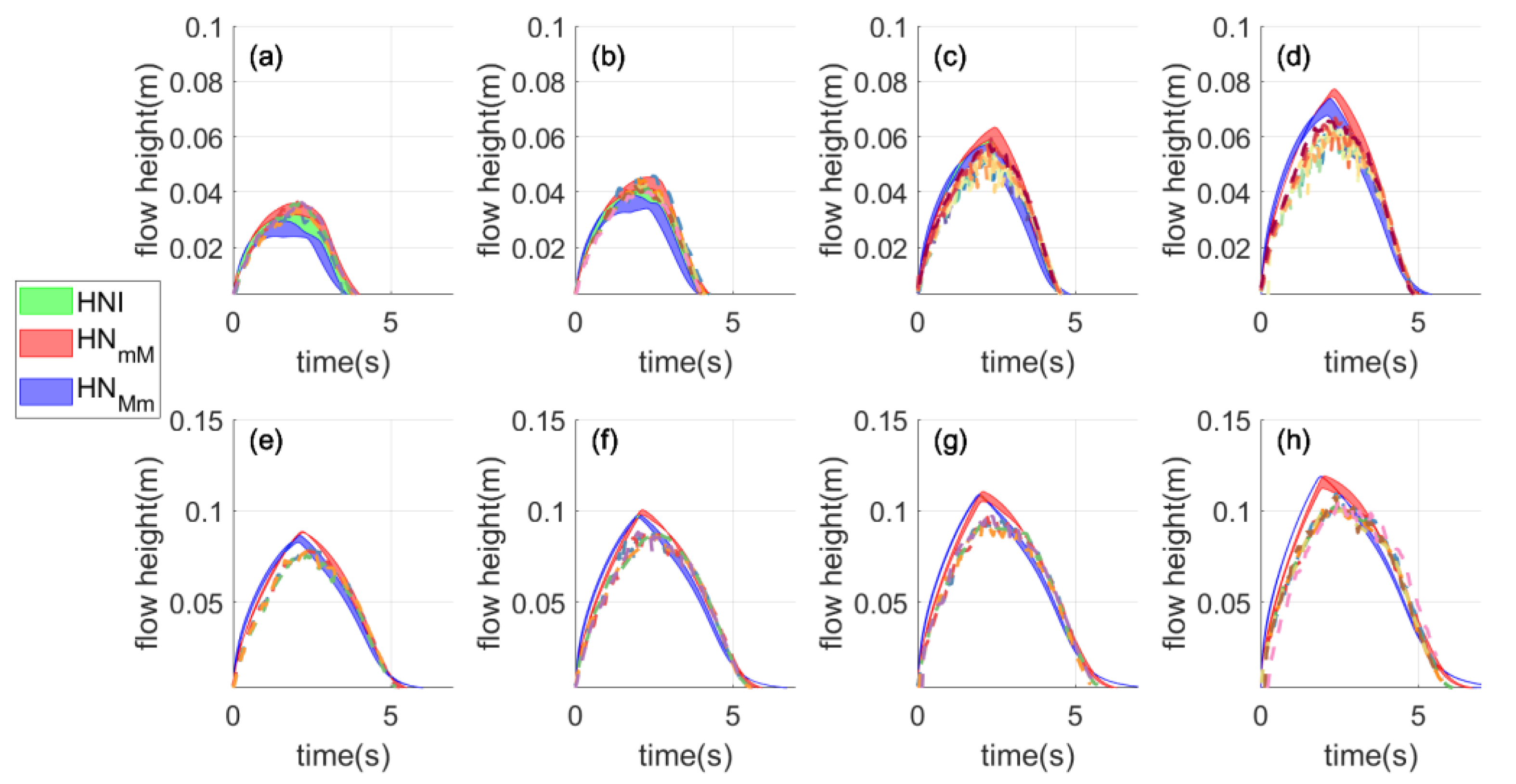
In this section, we present experimental and numerical time series of the flow height at the position P2, with time origin taken at the flow arrival time. More precisely, we provide graphs representing how the flow height changes in P2 during the whole process where the flow first runs along the slope up to a maximum distance and then comes back as a reverse flow. The simulations are carried out within the limits of friction coefficients nmin = 0.0125 s m−1/3 and nmax =0.0225 s m−1/3 for the slope and with various h1 values: h1 = 1, 2, 3, 4, 5, 6, 7, 8 mm. For a better representation of the results, instead of plotting the curves corresponding to all possible combinations of the parameters n and h1, we consider the two areas swept by all curves sharing the minimum (nmin ) and the maximum (nmax) value of the Manning’s coefficient and denote them by HNm and HNM, respectively. In Figure 5, we plot distinctly the intersection of such areas HNI (HNm ∩ HNM) and the relative complements HNmM (HNm − HNM) and HNMm (HNM − HNm).
The time interval of the process is captured quite well by the numerical model. Based on the width of the two curves, it can be seen that the heights of h1 has some influence on the flow height when the initial basin water level h0 is low, and that this influence gradually decreases. Comparing these curves with experimental data, one may observe that the model underestimates the flow height when the initial basin height is small and, vice-versa, it overestimates it when the basin level is high. As for the influence of n, considering that the overall trend of HNmM agrees better with the data (dashed lines) in the upslope and downslope part of the curves, one may conclude that the choice of n = 0.0125 s m−1/3 is better in capturing the height evolution profiles at P2.
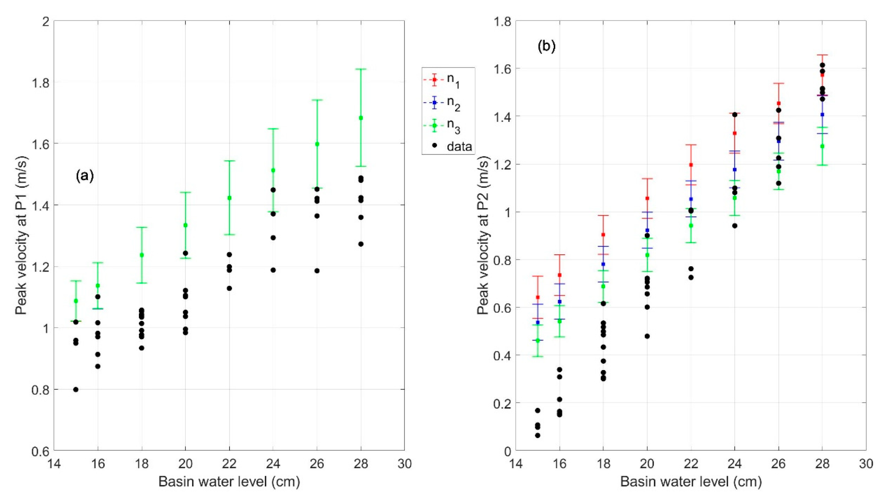
5.1.3. Peak Velocity at P1 and P2
The flow formed by the gate opening moves with the maximum velocity at the bore front, which is a region affected by high turbulence (see Bressan et al. [22]). Such a region is hard to catch properly in the calculations since the velocity appears as a step function. The peak velocities taken at the DV1 (position P1) and along the slope (position P2) are compared with the observed data under various numerical configurations in Figure 6a,b, respectively. To reduce turbulence noise, the experimental data have been smoothed by a cubic spline approximation. Three different values of friction coefficients have been considered for the slope (n1 = 0.0125 s m−1/3, n2 = 0.0175 s m−1/3, and n3 = 0.0225 s m−1/3) and for each friction coefficient, different h1 values have been implemented, which allows us to obtain peak velocity mean values with associated error bars, as shown in Figure 6.
By looking at the error bars, one can deduce that peak velocities are sensitive to the variation of h1, no matter the change of the basin water level. For the peak velocity at P1, the numerical model generally overestimates the flow velocity. Instead, the model provides reasonable peak velocity at P2 when the initial basin water level is higher than 0.24 m.
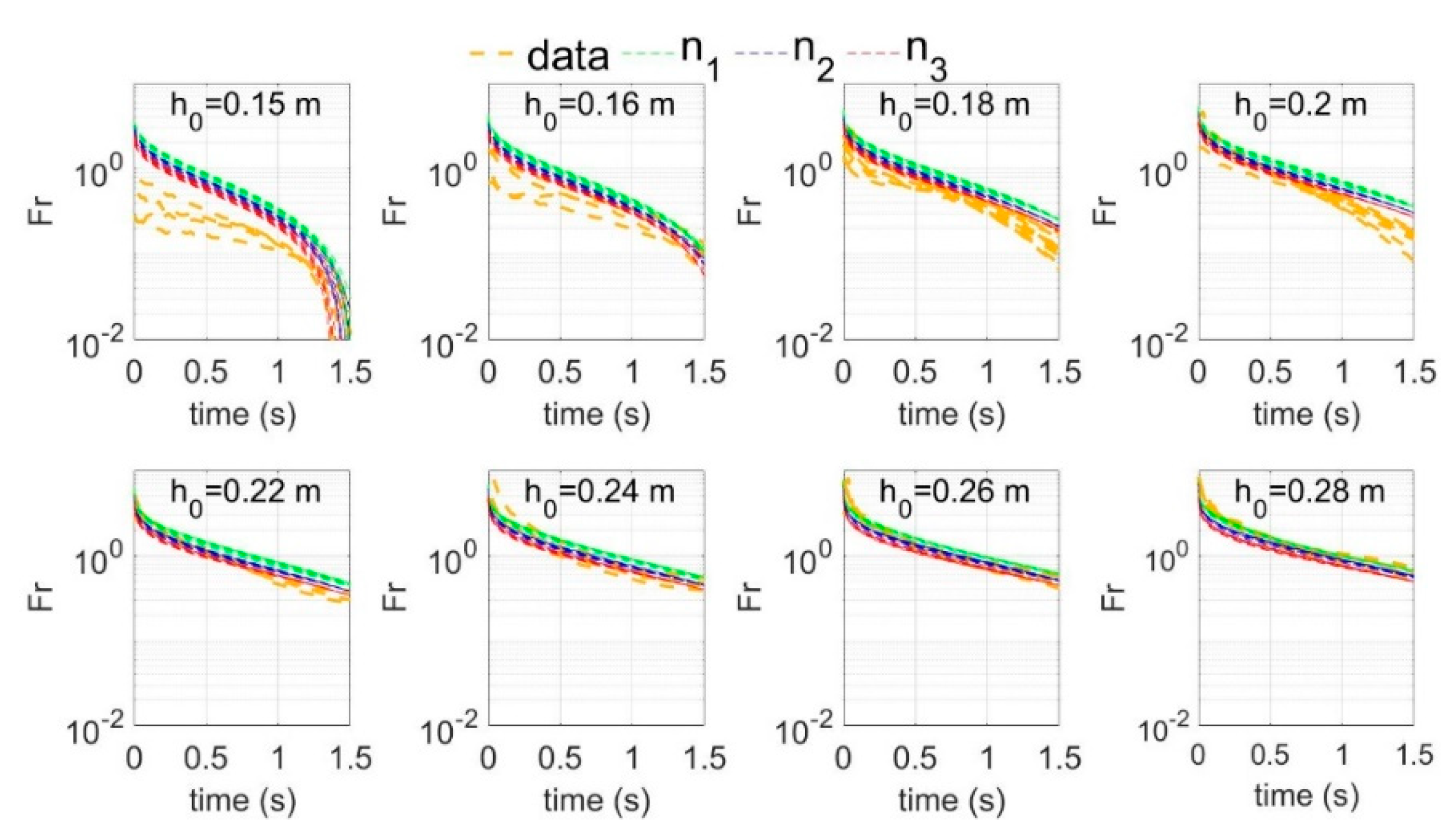
5.1.4. Froude Number at Position P2
A flow and its impact power can be characterized by the Froude number as was underlined by the observations of snow avalanches by Sovilla et al. [33]. Here, the Froude number Fr, defined as the ratio v/(gh)1/2 (v, h, and g being the flow velocity, height, and the gravity acceleration), is used to compare numerical and experimental data. The heights and velocities of the arrival flows are computed at position P2. Curves of Froude numbers vs. time are given in Figure 7. It may be seen that in all cases, Fr is a monotonic decreasing function of time, with the maximum value at the initial time, and that it passes from supercritical to subcritical values. This is due to the fact that when the bore arrives at the measuring point, its front has the minimum height and the maximum velocity, and therefore the corresponding Fr value is very high. In general, our numerical model overestimates the Froude number when h0 is smaller than 0.2 m, while it locates it at a reasonable range for higher values of h0. Notice that hereafter we will disregard the bore front region where the flow height is extremely low, i.e., smaller than 0.003 m since, as already noted in the previous section, experimental and numerical velocity data may be unreliable here.
5.2. Flows with Block
To model a condition where the water flow interacts with a block, we represent the block as a topographical relief and the impacting flow property is investigated by numerically monitoring the grid node placed in front of the block at a distance of 2 cm. The velocity is set to zero in all the nodes along the block surface. Considering the experiments of the quasi-cube block with dimensions 2.95 × 3.10 × 3.00 cm (length, width, height), the block topography is simplified as a cubic hump, 2.95 cm long and 3.00 cm high.
The time intervals between the instant of the flow arrival at the block and the instant of the instability onset are extracted from the experimental data and are shown in Table 1. There are three experimental cases for the configuration of h0 = 15 cm and seven cases for the other configurations. Considering the data, one can distinguish three different dynamic conditions, i.e., block stability (h0 = 15 cm), block probable stability (h0 = 16 and 17 cm), and block instability (h0 > 17 cm).
Based on these data and on data plotted in the instability graph that will be shown later, one can conclude that the present numerical model combined with the hydraulic formula related to a higher drag coefficient (CD = 6) might provide reasonable results to predict the minimum flow conditions for the block mobilization. A further relevant consideration is that the block destabilization, if occurs, takes place in the very first moments of the flow attack, with the delay interval getting shorter and shorter as the initial level of the water in the tank increases. Mobilization occurs much before the instant when the flow reaches the peak height (which occurs around 2 s after the flow arrival as shown in Figure 5). This suggests that to provide very accurate predictions on block stability or instability any numerical model needs to reproduce the time series of the bore transit especially in the very beginning, that is soon after the arrival of the bore front.
5.2.1. Flow Height Profiles
The experimental settings cover the range of the experimental flow from the situation where the flow is unable to mobilize the block to the situation where the flow breaks the block balance and moves it. In this section we compare numerical and experimental data under different configurations. The flow information is extracted from the node placed 2 cm ahead of the block in the numerical simulations.
From Figure 8, it can be seen that the introduction of the block on the flow path modifies the flow height in front of the block, especially when the flow is not strong (namely for smaller values of h0). We note further that the numerical model overestimates the flow height in the initial (0.5 s long) phase mainly because of the existence of the fix 1D boundary that represents the block. Interestingly, the experimental results computed without (NWB) and with the block (NWTB) are shown between the curves. Also noticeable is that, when h0 = 0.17 m and h0 = 0.18 m, NWB is capable of capturing the evolution of the flow height quite well (see Figure 8c,d). This ability is proven also for higher values of h0, whose graphs are however omitted here. These results show that the influence of the block on the flow height is negligible when the initial basin level is sufficiently large to mobilize the block soon.
5.2.2. Flow Conditions in Front of the Block
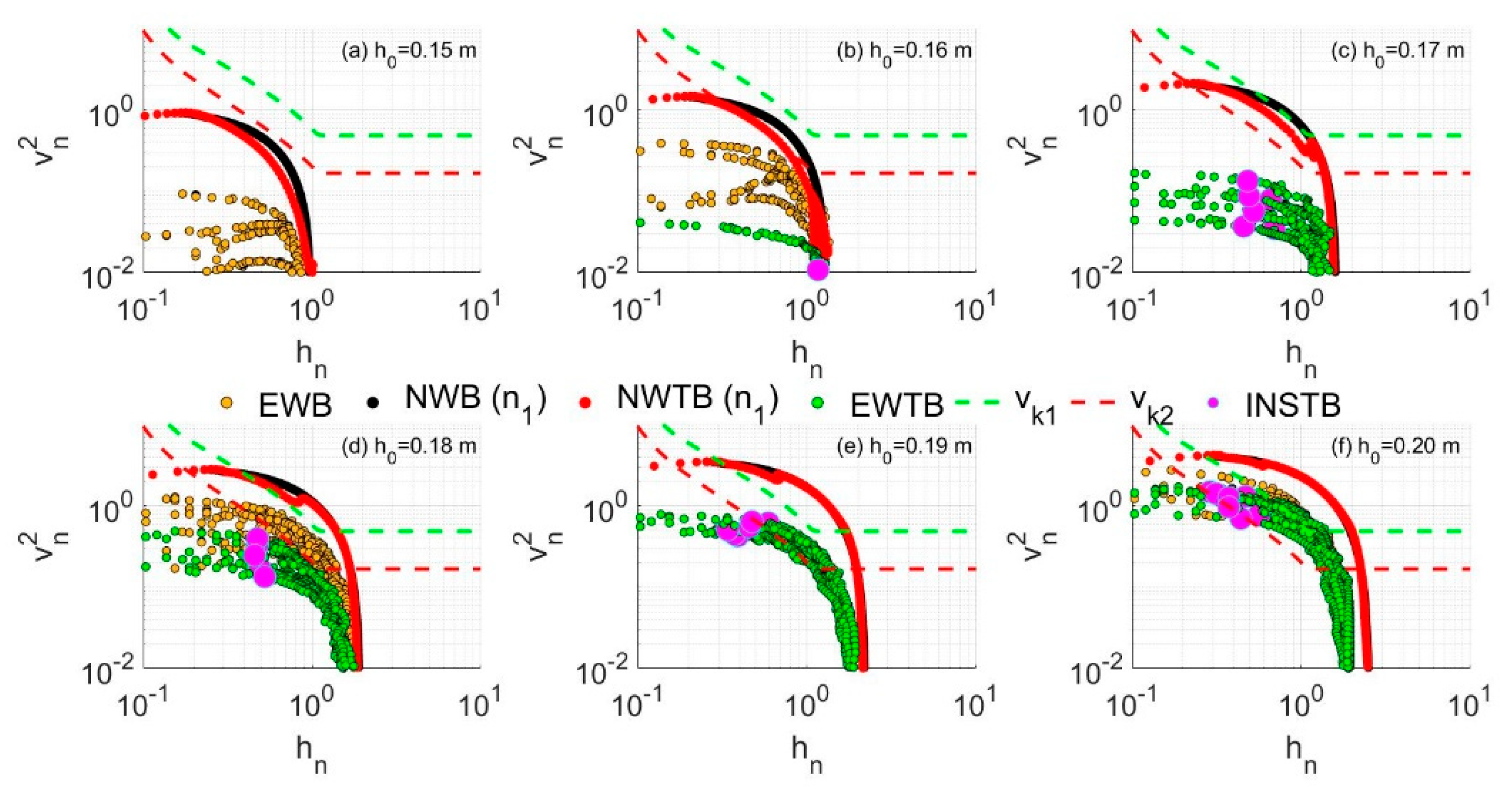
Experimental and numerical data of the flow measured in P2, that is the position 2 cm back from where the block will be placed, are displayed on the theoretical instability graph shown in Figure 9. For each single case, the diagram is built by plotting the values of the normalized flow velocity square vs. the normalized flow height only for the various instants during the bore advancement. The corresponding data related to the backflow are omitted. Each case is then represented by a set of points (numerical and experimental) corresponding to different times. In a sense, the time can be thought to evolve from left to right in the diagram while the flow height is increasing. The points in the leftmost region of the graph (smallest flow height) refer therefore to the initial stage of the flow, whereas the points with the largest flow height refer to the central stage of the flow (usually around 2 s, see Figure 5) where the flow attains the highest peak value. Considering the nearly-monotonic shape of all curves, that are almost flat at the beginning and then exhibit an increasing negative gradient, one deduces that in general (i) the impacting flow arrives with high velocity and low height, (ii) the flow velocity keeps nearly stable while the flow height gradually increases and then (iii) the flow decelerates rapidly with the end of the run-up process.
In the diagram we compare experimental and numerical results without a block and with a block. For the shown numerical runs the Manning’s coefficient is chosen as n1 = 0.0125 s m−1/3. Using data of Table 1, we are able to identify the flow properties exactly at the block destabilization instant. These are shown as INSTB dots (instability dots) in Figure 9.
Considering the numerical curves, we see that the cases with and without block differ only slightly for all values of h0, the discrepancy being higher for lower values. Even the experimental data show a difference between the block-yes and block-no cases that tend to decrease with the increase of h0, but the discrepancy is much larger especially for the smallest values of h0 (see e.g., graphs (a) and (b) of Figure 9). By comparing simulations and laboratory data, one notes that numerical curves are always external and embrace the observations, which means that they overestimate the flow velocity in the leftmost section of the graph and overestimate the flow height when velocities are small.
Looking at the instability graph, one reaches the conclusion that our results predict that the numerical flow will make the block unstable when h0 is higher than 0.18 m (CD = 2), or higher than 0.16 m (CD = 6). On the other hand, experimental data show that the onset of the block instability (marked with the solid dots INSTB in Figure 9) occurs in several cases within the stability region of the diagram. This is especially true for h0 = 0.16 m and h0 = 0.17 m, while for higher values of h0 the destabilization takes place at the boundary of the instability domain.
It is further worth noting that the block is mobilized when the flow height approximates the threshold of 4–5/10 of the boulder height (except for the data in h0 = 0.16 m), observation that has been also reported by Bressan et al. [22]. This may indicate that the flow height can significantly contribute to some hydraulic forces when it reaches such a limit.
6. Discussion and Conclusions
The processes of boulders transport are important to study sedimentology, hazard assessment, and geophysical flow evolution. On the basis of freely available data by Bressan et al. [22] of the incipient motion of a block acted by experimentally generated flows, a 1D shallow water numerical model was developed and used to explore the model capability and to improve our understanding of the processes. We analyzed experimental data that refer to two conditions, namely of bores propagating on a slope and bores impacting a block placed on that slope. The experimental flows were generated by opening a gate of a water tank with initial water level in the tank sweeping a range sufficiently large to cover a reasonable interval of flow velocities and heights. The numerical model was found to reproduce quite well the propagation time of the bore in the flat portion of the flume, with discrepancies only found in the flume sector closer to the gate, that is in the region of bore formation, which however do not affect the analysis. In the slope, we found that the numerical model reproduces well the overall time series of the bore height from the first arrival to the final backflow phase. However, the numerical results show a slight overestimation of the bore height, larger for more energetic flows, that is for the ones generated by higher initial water levels. This overestimation persists even by changing the bottom friction coefficients along the slope in the model within reasonable limits. The reproduction of the height of flows impacting the block allows interesting considerations. To notice first is that both experimental and numerical data show that the influence of the block on the flow height evolution in the position just in front of the block is relevant for less energetic flows and tends to decrease when flows are generated with higher initial water levels. The explanation is simple, since more energetic flows are able to destabilize the block soon after hitting it, and after block mobilization they behave like in cases without block. Interestingly, when the flow is really perturbed by the presence of the block, i.e., in the first stage of the block attack for lower values of h0, empirical heights lie between heights simulated with block and without block. In a sense, it shows that the perturbation induced by the numerical block is overestimated, which is very likely because of the use of a 1D model, where the block is represented by a fix topography. Indeed, this implies that the flow is bound either to stop against the block or to flow above, but it is not allowed to go around the obstacle like it instead happens in the laboratory experiments.
As for the ability of the model to reproduce the experimental flow velocity on the slope, we found that results are less satisfactory than for the flow height. This is due to (1) the large spread of experimental data affected by high-frequency turbulence that imposes smoothing to get manageable velocity curves of the bore front, and also to (2) the fact that, as the simulated results show, the velocity profile along the bore is the highest in the front region and decreases gradually when moving away from the front. The consequence is that, like in a shock wave, the grid nodes in the neighborhood of the front pass from being dry (with zero velocity) to being wet (with high velocity) in a very short time. Though this situation is managed by the code and is no cause of numerical instabilities, the accuracy of the results may be less than desired.
With the above considerations in mind, let us focus on what we learned from the application of our numerical model to the laboratory data. The instability diagrams of the normalized flow square speed vs. the normalized flow height are useful since they allow one to compare simulated and experimental data locating them in the instability/stability domains identified by theoretical hydraulic formulas. When one puts all data related to a single case flow, that is to a single bore passage, on that graph, one sees that these data are arranged along a curve, which has a typical shape with a monotonic trend. It can be seen as a trajectory for a representative point of the flow in the phase space (). If we restrict to the phase of bore advancement, such point moves rightward starting from the left end of the trajectory, because when the bore front attacks the block its velocity is high whereas its height is very small. On the bi-log graphs these trajectories start almost horizontal from the vertical axis (which corresponds to a stage of almost constant bore speed and increasing bore height), then exhibit an increasing inclination until the horizontal axis is almost normal (which corresponds to the stage of maximum inundation height and vanishing velocity). The two end points, that is the intersections of the trajectory with the diagram axes, can be used to identify the trajectory. These kind of trajectories are associated with the way the bore is formed, that is through the dam-braking mechanism realized by manually releasing a gate. Increasing the level of water in the tank has the effect of producing more energetic bores that on the graph follow trajectories having end points more distant from the graph origin, so that one can establish a one-to-one relation between the level of water in the tank h0 and the pair of end points. All trajectories start on the stable part of the domain. If h0 is large enough and correspondingly the trajectory left end point is high enough, the trajectory may intersect the theoretical stability curve, which implies that the flow is able to mobilize the block. On the other hand, if h0 is too small the trajectory does not cross the stability curve at all, and the flow remains always in the stability region, being theoretically unable to displace the block. With this understanding, it is clear that the generation mechanism can produce flow trajectories that sweep a relevant area of the stability graphs but cannot enable one to fully explore the stability region. In particular, the stability domain characterized by low flow velocity and large flow height could be unreachable by such flow trajectories. To cover that region, the only strategy will be to increase the level h0, but this way the trajectory will start from an end point on the velocity axis high enough to enter the instability region, and the block will be mobilized. Therefore, to produce slow and high flow, one should consider other generation mechanisms, such as fluid circulation produced by hydraulics pumps where velocity and flow height are not correlated; one possibility could be to remove the water from the flume at the upper end of the slope and to re-input it on the other side of the flume at the beginning of the flat bottom sector, creating therefore a water circulation with controlled fluxes and volumes.
As for the block stability, we can highlight two relevant observations. First, we note that numerical trajectories computed with and without the block do not differ too much in the phase space of the system but are systematically above the set of points that describe the experimental trajectories. Second, looking at the experimental points in the phase space marking the onset of block mobilization, we may point out that all of them are well below the theoretical instability curves. This latter feature was already noted by Bressan et al. [22]. Their conclusions were that probably the theoretical curves are based on an over-simplified hydraulic model (not considering flow height that do not completely submerge the block), but more importantly that their experimental data were affected by high-frequency fluctuations due to turbulence, so that instability could have been caused by temporary velocity peaks, representing large deviations from the mean flow velocity. If one were able to plot these deviations in the stability graphs, the experimental points will appear shifted upward, that is closer to or even within the theoretical block instability region. Our numerical results confirm the validity of those conclusions. Indeed, the shallow water model cannot account for the flow turbulence, and in case of turbulent flow is only able to compute mean flow properties, but with a caveat. Turbulence is known to subtract energy to the mean flow since the total available energy should feed both features. On the other hand, the only way to subtract energy to the numerical mean flow is by means of bottom stresses. Our results show that changing the bottom friction in the flume does not modify significantly the computed flow, nor, as a consequence, the flow trajectory in the phase space. Therefore, bottom friction cannot be used to reduce the mean flow energy in a shallow water model as a substitute of a turbulence dissipation mechanism. This explains why, considering cases with the same initial water potential energy (i.e., cases with the same initial water level in the tank), numerical trajectories lie always above the corresponding experimental points. Further, it is worth to highlight, that, though with the limitations mentioned above, if we group results according to the initial water level, and we assess the instability from the intersection of the numerical with the theoretical curves, the predicted block instability respects almost fully the experimental data if we use the curve obtained with CD = 6, that is block stability for h0 = 15 cm, near instability for h0 = 16 cm and block mobilization for h0 larger than 16 cm.
As concluding remarks, we can state that combining laboratory experiments and the numerical analyses provides a very powerful strategy to interpret physical phenomena, and in our case to improve our understanding of the mobilization of boulders by hydraulic flows. In our study we found that simulations and laboratory data confirm that the destabilization of boulders, occurring when the mean flow dynamics in principle is unable to cause it, can be explained by the relevant role of temporary fluctuations of the flow velocity, that are able to move the representative point of the flow in the phase space of the system upward, from the block stability into the block instability region. It is relevant to add that our conclusions are based on the analysis of data of only one of the types of blocks taken into account by Bressan et al. [22], and further, that, due to the limitation of the numerical model, the instability of blocks is interpreted only in terms of the 1D interaction between the flow and the block. The complex interaction mechanisms taking place in a 3D system will be studied with more advanced numerical techniques in our further research. However, in spite of the formal limitations, we think that our present findings might have a general validity and can also be applied to many other block shapes.
Author Contributions
S.T. conceived the idea and L.B. provided the data. L.W. performed the simulations and wrote the first draft. All authors participated in the discussion and edition of the manuscript.
Funding
The research was partially financed by the FP7 Project ASTARTE “Assessment, Strategy and Risk Reduction for Tsunami in Europe” (FP7-ENV2013 6.4-3, Grant 603839).
Acknowledgments
The author Liang Wang greatly appreciates the financial support from the cooperation agreement between the University of Bologna and the China Scholarship Council.
Conflicts of Interest
The authors declare no conflicts of interest.
References
- Etienne, S.; Buckley, M.; Paris, R.; Nandasena, A.K.; Clark, K.; Strotz, L.; Chagué-Goff, C.; Goff, J.; Richmond, B. The use of boulders for characterising past tsunamis: Lessons from the 2004 Indian Ocean and 2009 South Pacific tsunamis. Earth Sci. Rev. 2011, 107, 76–90. [Google Scholar] [CrossRef]
- Scicchitano, G.; Monaco, C.; Tortorici, L. Large boulder deposits by tsunami waves along the Ionian coast of south-eastern Sicily (Italy). Mar. Geol. 2007, 238, 75–91. [Google Scholar] [CrossRef]
- Goto, K.; Okada, K.; Imamura, F. Characteristics and hydrodynamics of boulders transported by storm waves at Kudaka Island, Japan. Mar. Geol. 2009, 262, 14–24. [Google Scholar] [CrossRef]
- Kennedy, A.B.; Mori, N.; Zhang, Y.; Yasuda, T.; Chen, S.E.; Tajima, Y.; Pecor, W.; Toride, K. Observations and Modeling of Coastal Boulder Transport and Loading During Super Typhoon Haiyan. Coast. Eng. J. 2015, 58, 1640004. [Google Scholar] [CrossRef]
- Terry, J.P.; Dunne, K.; Jankaew, K. Prehistorical frequency of high-energy marine inundation events driven by typhoons in the Bay of Bangkok (Thailand), interpreted from coastal carbonate boulders. Earth Surf. Process. Landf. 2016, 41, 553–562. [Google Scholar] [CrossRef]
- Biolchi, S.; Furlani, S.; Antonioli, F.; Baldassini, N.; Causon Deguara, J.; Devoto, S.; Di Stefano, A.; Evans, J.; Gambin, T.; Gauci, R.; et al. Boulder accumulations related to extreme wave events on the eastern coast of Malta. Nat. Hazards Earth Syst. Sci. 2016, 16, 737–756. [Google Scholar] [CrossRef] [Green Version]
- Haehnel, R.B.; Daly, S.F. Maximum Impact Force of Woody Debris on Floodplain Structures. J. Hydraul. Eng. 2004, 130, 112–120. [Google Scholar] [CrossRef]
- Goto, K.; Sugawara, D.; Ikema, S.; Miyagi, T. Sedimentary processes associated with sand and boulder deposits formed by the 2011 Tohoku-oki tsunami at Sabusawa Island, Japan. Sediment. Geol. 2012, 282, 188–198. [Google Scholar] [CrossRef]
- Major, J.J. Pebble orientation on large, experimental debris-flow deposits. Sediment. Geol. 1998, 117, 151–164. [Google Scholar] [CrossRef]
- Blair, T.C.; McPherson, J.G. Grain-size and textural classification of coarse sedimentary particles. J. Sediment. Res. 1999, 69, 6–19. [Google Scholar] [CrossRef]
- Shanmugam, G. Process-sedimentological challenges in distinguishing paleo-tsunami deposits. Nat. Hazards 2012, 63, 5–30. [Google Scholar] [CrossRef]
- Jakob, M. Debris-flow hazard analysis. In Debris-Flow Hazards and Related Phenomena; Jakob, M., Oldrich, H., Eds.; Springer: Berlin/Heidelberg, Germany, 2005; pp. 411–437. [Google Scholar]
- Ceccato, F.; Redaelli, I.; di Prisco, C.; Simonini, P. Impact forces of granular flows on rigid structures: Comparison between discontinuous (DEM) and continuous (MPM) numerical approaches. Comput. Geotech. 2018, 103, 201–217. [Google Scholar] [CrossRef]
- Hsiao, S.C.; Lin, T.C. Tsunami-like solitary waves impinging and overtopping an impermeable seawall: Experiment and RANS modeling. Coast. Eng. 2010, 57, 1–18. [Google Scholar] [CrossRef]
- Cui, P.; Zeng, C.; Lei, Y. Experimental analysis on the impact force of viscous debris flow. Earth Surf. Process. Landf. 2015, 40, 1644–1655. [Google Scholar] [CrossRef] [Green Version]
- Nouri, Y.; Nistor, I.; Palermo, D.; Cornett, A. Experimental Investigation of Tsunami Impact on Free Standing Structures. Coast. Eng. J. 2010, 52, 43–70. [Google Scholar] [CrossRef]
- Nandasena, N.A.K.; Paris, R.; Tanaka, N. Reassessment of hydrodynamic equations: Minimum flow velocity to initiate boulder transport by high energy events (storms, tsunamis). Mar. Geol. 2011, 281, 70–84. [Google Scholar] [CrossRef]
- Nott, J. Extremely high-energy wave deposits inside the Great Barrier Reef, Australia: Determining the cause-tsunami or tropical cyclone. Mar. Geol. 1997, 141, 193–207. [Google Scholar] [CrossRef]
- Imamura, F.; Goto, K.; Ohkubo, S. A numerical model for the transport of a boulder by tsunami. J. Geophys. Res. Ocean. 2008, 113, 1–12. [Google Scholar] [CrossRef]
- Nandasena, N.A.K.; Paris, R.; Tanaka, N. Numerical assessment of boulder transport by the 2004 Indian ocean tsunami in Lhok Nga, West Banda Aceh (Sumatra, Indonesia). Comput. Geosci. 2011, 37, 1391–1399. [Google Scholar] [CrossRef]
- Nandasena, N.A.K.; Tanaka, N. Boulder transport by high energy: Numerical model-fitting experimental observations. Ocean Eng. 2013, 57, 163–179. [Google Scholar] [CrossRef]
- Bressan, L.; Guerrero, M.; Antonini, A.; Petruzzelli, V.; Archetti, R.; Lamberti, A.; Tinti, S. A laboratory experiment on the incipient motion of boulders by high-energy coastal flows. Earth Surf. Process. Landf. 2018, 43, 2935–2947. [Google Scholar] [CrossRef] [Green Version]
- Savage, S.B.; Hutter, K. The motion of a finite mass of granular material down a rough incline. J. Fluid Mech. 1989, 199, 177–215. [Google Scholar] [CrossRef]
- Louaked, M.; Hanich, L. TVD scheme for the shallow water equations. J. Hydraul. Res. 1998, 36, 363–378. [Google Scholar] [CrossRef]
- Tinti, S.; Tonini, R. The UBO-TSUFD tsunami inundation model: Validation and application to a tsunami case study focused on the city of Catania, Italy. Nat. Hazards Earth Syst. Sci. 2013, 13, 1795–1816. [Google Scholar] [CrossRef]
- Brufau, P.; Vazquez-Cendon, M.E.; Garcia-Navarro, P. A numerical model for the flooding and drying of irregular domains. Int. J. Numer. Meth. Fluids 2002, 39, 247–275. [Google Scholar] [CrossRef]
- Nessyahu, H.; Tadmor, E. Non-oscillatory central differencing for hyperbolic conservation laws. J. Comput. Phys. 1990, 87, 408–463. [Google Scholar] [CrossRef] [Green Version]
- Tai, Y.C.; Noelle, S.; Gray, J.M.N.T.; Hutter, K. Shock-capturing and front-tracking methods for granular avalanches. J. Comput. Phys. 2002, 175, 269–301. [Google Scholar] [CrossRef]
- Wang, Y.; Hutter, K. Comparisons of numerical methods with respect to convectively dominated problems. Int. J. Numer. Methods Fluids 2001, 37, 721–745. [Google Scholar] [CrossRef]
- Wang, L.; Zaniboni, F.; Tinti, S.; Zhang, X. Reconstruction of the 1783 Scilla landslide, Italy: Numerical investigations on the flow-like behaviour of landslides. Landslides 2019, 16, 1065–1076. [Google Scholar] [CrossRef]
- Noormets, R.; Crook, K.A.W.; Felton, E.A. Sedimentology of rocky shorelines: 3. Hydrodynamics of megaclast emplacement and transport on a shore platform, Oahu, Hawaii. Sediment. Geol. 2004, 172, 41–65. [Google Scholar] [CrossRef]
- Paris, R.; Fournier, J.; Poizot, E.; Etienne, S.; Morin, J.; Lavigne, F.; Wassmer, P. Boulder and fine sediment transport and deposition by the 2004 tsunami in Lhok Nga (western Banda Aceh, Sumatra, Indonesia): A coupled offshore-onshore model. Mar. Geol. 2010, 268, 43–54. [Google Scholar] [CrossRef]
- Sovilla, B.; Schaer, M.; Kern, M.; Bartelt, P. Impact Pressures and flow regimes in dense snow avalanches observed at the Vallée de la Sionne test site. J. Geophys. Res. Earth Surf. 2008, 113, 1–14. [Google Scholar] [CrossRef]
- Te Chow, V. Open-Channel Hydraulics; McGraw-Hill: New York, NY, USA, 1959. [Google Scholar]
Figure 1.
Experimental setup: The generated flow moves from left to right after the opening of the gate. The water level sensors WL1, WL2, WL3 are placed at the respective horizontal distances of 0.16, 0.28, and 1.94 m from the gate. The Doppler ultrasound velocimeter DV1 is placed at 2.7 m from the gate and at 0.4 m from the slope base, pointing at the incoming bore. DV2 and DV3 are placed at the distance of 1.09 m along the slope with respect to the slope base. The boulder is located 2 cm away from the DV2 and DV3 upslope.

Figure 2.
Sketch of forces and torques acting on a partially submerged block located on a slope of incline angle θ. Letters W, D, F, L denote weight, drag force, friction force, and lift force respectively. B is the center of mass and AM is the rotation axis. In computations, all forces are applied to the center of mass of the block B and all torques are computed with respect to the rotation axis passing through AM (after Bressan et al. [22]).

Figure 3.
Theoretical instability graph: flow square velocity vs. flow height, where the flow height hn is normalized to the height of the boulder hboulder and the square velocity is normalized to ghboulder. Curves are calculated for a block of 2.95 × 3.10 × 3.00 cm (length, width and height). Each curve divides the domain into a stability (below) and instability (above) region for the boulder. Subscripts M and k represent curves derived from rotational and translational inequality formulas. The three vertical dash lines on the graph from left to right represent the flow depth when (1) the bottom, (2) the front, and (3) the top surfaces of the block are fully submerged.

Figure 4.
Propagation times of the bore derived from WL experimental and synthetic records for different values of the initial water height h0. For each value of h0, the value of h1 has been varied from 1 to 8 mm in the numerical runs. The adopted Manning’s coefficient is n1 = 0.0125 s m−1/3.
Figure 4.
Propagation times of the bore derived from WL experimental and synthetic records for different values of the initial water height h0. For each value of h0, the value of h1 has been varied from 1 to 8 mm in the numerical runs. The adopted Manning’s coefficient is n1 = 0.0125 s m−1/3.

Figure 5.
Flow height profiles at position P2; (a–h) refer to different basin water levels; h0 = 0.15, 0.16, 0.18, 0.20, 0.22, 0.24, 0.26, 0.28 m. Dash lines are the experimental data.
Figure 5.
Flow height profiles at position P2; (a–h) refer to different basin water levels; h0 = 0.15, 0.16, 0.18, 0.20, 0.22, 0.24, 0.26, 0.28 m. Dash lines are the experimental data.

Figure 6.
Peak flow velocities at (a) P1 and (b) P2. Numerical results for P1 are obtained with the friction coefficient n = 0.0125 m−1/3 s, while for P2 are obtained by using different coefficients on the slope (n1 = 0.0125 m−1/3 s, n2 = 0.0175 m−1/3 s, n3 = 0.0225 m−1/3 s). Error bars cover the full range of values obtained by varying h1 for a given n.

Figure 7.
Froude number evolution at P2. Yellow dash lines are experimental data. The green, blue, and red lines refer to Manning’s coefficients n1 = 0.0125 m−1/3 s, n2 = 0.0175 m−1/3 s, and n3 = 0.0225 m−1/3 s, respectively. Curves are displayed in the first 1.5 s because in all the cases in which the block was unstable (see Table 1) mobilization occurred within this time interval.

Figure 8.
Flow height profiles for the cases with basin level from h0 = 0.15 m to h0 = 0.18 m (denoted from (a) to (d)). Here, WB and WTB denote the configuration “without block” and “with the block” respectively. The initial capital ”N” and ”E” denote data from numerical simulations and experiments respectively. The displayed “EWB” data are obtained by averaging the original data sets. NWTB are omitted in plots (c) and (d), considering that NWB is able to capture the experimental data (the block was initialized soon as can be seen in Table 1).

Figure 9.
Instability diagram with experimental and numerical data of the cases from h0 = 0.15 m to h0 = 0.20 m, denoted from (a) to (f) in subfigures (vk1 and vk2 are the calculated instability velocities for CD = 2 and CD = 6). For the meaning of EWB, NWB, EWTB and NWTB see caption of Figure 8. When the initial water basin is higher, the influence of the block on the impacting flow is not so large. However, the block significantly contributes to the reduction of the flow velocity (see (b) and (d)), which has not been reproduced by the numerical model. The INSTB dots represent the flow properties at the exact moment when the block is mobilized. We neglect some flow velocity data for the case of h0 = 0.16 m since they are really chaotic.


Table 1.
Time interval (in seconds) between the flow arrival time and the time of block instability.
Table 1.
Time interval (in seconds) between the flow arrival time and the time of block instability.
| h0 (cm) | 15 | 16 | 17 | 18 | 19 | 20 |
|---|---|---|---|---|---|---|
| Case 1 | stable | 0.51 | stable | 0.17 | 0.19 | 0.12 |
| Case 2 | stable | stable | 0.34 | 0.20 | 0.15 | 0.16 |
| Case 3 | stable | 1.02 | 0.21 | 0.18 | 0.13 | 0.09 |
| Case 4 | stable | 0.30 | 0.22 | 0.11 | 0.08 | |
| Case 5 | stable | 0.37 | 0.18 | 0.10 | 0.12 | |
| Case 6 | stable | 0.22 | 0.16 | 0.17 | 0.11 | |
| Case 7 | stable | 0.22 | 0.25 | 0.13 | 0.14 |
© 2019 by the authors. Licensee MDPI, Basel, Switzerland. This article is an open access article distributed under the terms and conditions of the Creative Commons Attribution (CC BY) license (http://creativecommons.org/licenses/by/4.0/).
Share and Cite
MDPI and ACS Style
Wang, L.; Bressan, L.; Tinti, S. Numerical Investigations on the Instability of Boulders Impacted by Experimental Coastal Flows. Water 2019, 11, 1557. https://doi.org/10.3390/w11081557
AMA Style
Wang L, Bressan L, Tinti S. Numerical Investigations on the Instability of Boulders Impacted by Experimental Coastal Flows. Water. 2019; 11(8):1557. https://doi.org/10.3390/w11081557
Chicago/Turabian StyleWang, Liang, Lidia Bressan, and Stefano Tinti. 2019. "Numerical Investigations on the Instability of Boulders Impacted by Experimental Coastal Flows" Water 11, no. 8: 1557. https://doi.org/10.3390/w11081557
Note that from the first issue of 2016, this journal uses article numbers instead of page numbers. See further details here.