Article

The Relative Importance of Spatial Scale Variables for Explaning Macroinvertebrate Richness in Different Aquatic Ecological Function Regions

1
State Key Laboratory of Environmental Criteria and Risk Assessment, Chinese Research Academy of Environmental Sciences, Beijing 100012, China
2
Laboratory of Riverine Ecological Conservation and Technology, Chinese Research Academy of Environmental Sciences, Beijing 100012, China
*
Authors to whom correspondence should be addressed.
Water 2019, 11(8), 1550; https://doi.org/10.3390/w11081550
Submission received: 31 March 2019 / Revised: 22 July 2019 / Accepted: 23 July 2019 / Published: 26 July 2019
(This article belongs to the Section Water Quality and Contamination)

Abstract

:
Identifying the key drivers of aquatic fauna structuring at multiple spatial scales is critical in reducing biodiversity loss. Macroinvertebrates are the most sensitive indicators of disturbance and they are used as a cost-effective tool for bioassessment at catchment and site scales. The focus of our study was to identify the key drivers from three classes of environmental variables (geophysical landscape, land use, and site habitat) that influence macroinvertebrate richness in different aquatic ecological function regions (AEFRs) of the Liaohe River Basin. We sampled macroinvertebrate assemblages, extracted geophysical and climate variables from geospatial data, and quantified physical and chemical habitats from 407 randomly distributed sites that belong to the three level-I AEFRs. We analyzed our data through multiple linear regression models by using the three classes of predicted variables alone and in combination. The models that were constructed in the first level-I AEFR explained similar amounts of macroinvertebrate richness and had the maximum ability to explain how macroinvertebrate richness distributed (denoted “explaining ability”; geophysical landscape: RGL2 ≈ 60%, land use and site habitat: RLU2 and RSH2 ≈ 50%, and combined: RCB2 ≈ 75%). The explaining abilities for the third level-I AEFR were as follows: RGL2 ≈ 11%, RLU2 ≈ 14%, RSH2 ≈ 25%, and RCB2 ≈ 38%. The explaining abilities for the 4th level-I AEFR were as follows: RGL2 ≈ 30%, RLU2 ≈ 7%, RSH2 ≈ 40%, and RCB2 ≈ 55%. We conclude that: (1) all of the combined models explained more interaction as compared with the single models; (2) the environmental variables differed among different level-I AEFRs; and, (3) variables in the site habitat scale were the most robust explainers when analyzing the relationship between environmental variables and macroinvertebrate richness and they can be recommended as the optimal candidate explainer. These results may provide cost-effective tools for distinguishing and identifying the drivers of sensitive aquatic organisms at regional scales.

1. Introduction

Freshwater ecosystems provide irreplaceable ecological functions for human beings, including diluting contaminants and providing energy and water supply for irrigation and aquaculture. In addition, they maintain high biodiversity, supporting nearly 12% of the total species richness [1,2]. Nevertheless, the biodiversity of freshwater ecosystems is the most threatened, and some researchers indicate that the species extinction speed is five times higher than in every other community [3]. Species richness has been used as a useful indicator for measuring biodiversity, and identifying the distribution pattern and the key environmental variables that affect it at various spatial scales is essential in preventing biodiversity loss and formulating effective conservation actions in freshwater ecosystems [4,5,6,7]. Benthic macroinvertebrates are often used for the biological assessment of changes in response to environmental conditions—such as mobility, morphology, physiology, taxa sensitivity to disturbance, and the continuum response to environmental variables [8,9,10,11,12,13]—in freshwater ecosystems via single and multiple index and predicted models [12,14].
Researchers have claimed that the climate, geology, and topography at large scales can influence geomorphic processes and control the nutrient input, riparian habitat, and water quality at smaller scales, especially the reach and site scales, and the aquatic fauna via various and complicated pathways [15,16,17,18]. Land use, from undisturbed to human-dominated landscapes, represents anthropogenic disturbance at the catchment scale, and it has been used for decades to illustrate the direct and indirect anthropogenic effects on freshwater ecosystems [19,20,21,22,23,24]. Previous studies have documented that land use can affect the function and processes of freshwater ecosystems through various pathways, including hydrological alteration [25], riparian clearing [26], loss of woody debris [27], input of excess sedimentation, and nutrient and containment [28,29,30], all of which affect the quality and availability of site habitats for aquatic organisms [7]. Physical and chemical variables have a key impact on aquatic assemblages, owing to the greater direct effects of site-scale variables compared with catchment-scale [31]. However, because smaller scale variables are always structured by the larger scale variables, it is difficult to identify the relative importance of each variable on aquatic communities [7]. Nevertheless, researchers can determine the key factors that structure assemblages with the help of the increasing the availability of digitization of landscape variables at the catchment scale [7].
Previous studies have focused on the interaction of variables at various scales with aquatic organisms, especially fish and macroinvertebrates, in headwaters and the whole catchment [7,24,32]. The differences between geophysical variables, land use, and human impacts among different ecoregions have not been received much attentions in previous research [33]. Ecoregions are the management units that divide the whole catchment into different units that are based on the characteristics of territorial environmental driving factors, including landform, agrotype, climate, natural vegetation, and land use [34,35,36,37,38,39]. The ecoregions highlight the significant heterogeneity features among different aquatic ecological regions; however, similarities in water quality and aquatic organisms exist within one ecoregion. Thus, we predicted that different sets of environmental variables would explain the richness in each ecoregion.
The Liaohe River Basin, which is the seventh largest watershed in northeast China, covers more than 2.2 × 10⁵ km2, and it mainly experiences a temperate semi-humid and semi-arid monsoon climate. This watershed has become a hotspot for biodiversity conservation efforts in recent years, owing to the extinction of large endemic fish species (approximately half of the historically present species currently exist) and the loss of biodiversity that are associated with degraded water quality and physical habitat quality as a result of intense deforestation and a transformation from underdeveloped to agricultural and urban land use [40,41,42,43]. Researchers have partitioned the whole Liaohe River Basin into four level-I aquatic ecological function regions to manage the natural resources more scientifically and reasonably (hereafter, AEFRs, Figure 1, unpublished data), which are based on identifying the heterogeneous features of structure and function of aquatic ecosystems at the catchment scale. The objectives of the current paper were to identify the relative importance of environmental variables at the catchment and site scales individually and combined for macroinvertebrate richness in every AEFR of the Liaohe River Basin, and to identify the model that would best explain more variability.

2. Methods

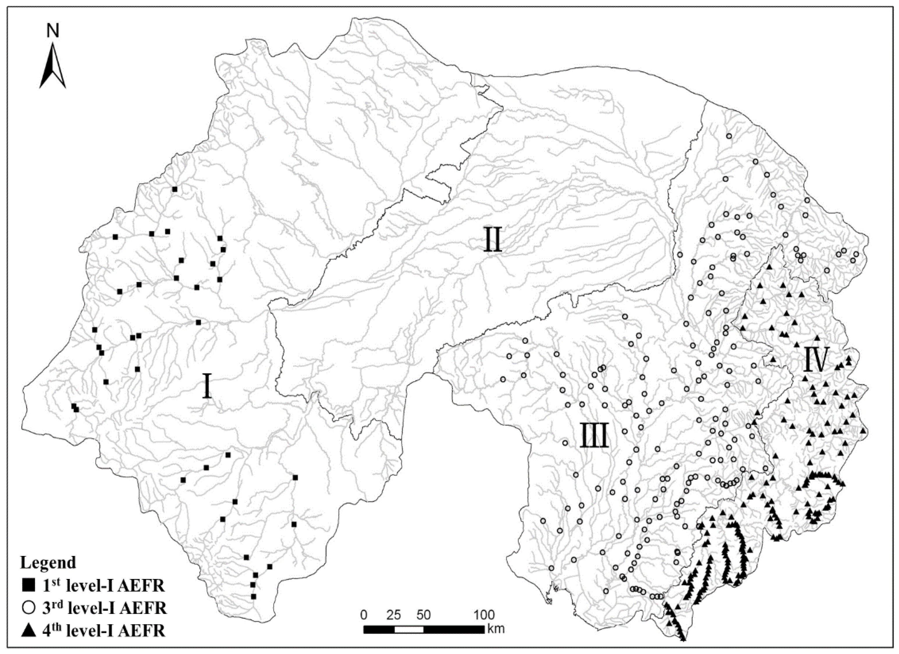
2.1. Study Area and Site Selection

The Liaohe River Basin (40°30′–45°10′ N, 117°00′–125°30′ E) is composed of two independent separate hydrographic nets, the Da-Liao and Hun-Tai River systems, which flow into the Bohai Sea. The topography is composed of 48.2% mountains, 21.5% hills, 24.3% plains, and 6% sand, and the major stems and tributaries total 1430 km. The maximal drop in altitude is more than 1200 m, decreasing from piedmont in a west and southeast direction to the central plain, which is called the Liaohe River Plain, where the large and medium-size cities and major grain-producing areas in Liaoning Province are distributed. Annual rainfall decreases from the southeast to the northwest and ranges from 900 to 350 mm [42]. The area belonging to the second level-I AEFR has been experiencing drought for years and it is not included in the study. In the upper area of the Da-Liao and Hun-Tai Rivers, grass and forests dominate the land use, respectively, whereas the land use where the Liaohe River Plain is located is dominated by intensive agriculture and urban use [41,43].
A total of 407 sampling sites were randomly selected and distributed evenly as much as possible (Figure 1): 36, 169, and 202 in the first, third, and fourth level-I AEFRs, respectively. Macroinvertebrate, substrate, and water samples were collected in a 100 m stream reach for each site. Sampling for the first and third level-I AEFRs was conducted from late August to late September in 2012 and 2013, and for the fourth level-I AEFR sampling was conducted from May 2009 to August 2010.

2.2. Geophysical Landscape Variables

The accurate point coordinates and altitude for each site were measured using a portable GPS (Explorist-200, Magellan, San Dimas, CA, USA) in situ. The slope, sinuosity, and stream order were calculated from the digital elevation model (DEM) datum within 90 m resolution and a geomorphic type vector diagram of Liaohe River Basin at a scale of 1:100,000. The DEM datum was downloaded from the USGS website (http://srtm.usgs.gov). The drainage network of the Liaohe River Basin was extracted from a DEM based on a ground water overflow model. All of the rivers were divided into segments on the basis of the setting of an intersection as the break point, and the intersection was determined by visualization. Reach length, slope, sinuosity, and stream order for each site were obtained from the specified river segment. The slope was automatically extracted by inputting relevant data into the slope calculation tool in surface analysis based on the DEM layers data. Sinuosity was calculated by the ratio value between the physical and straight length for each river segment. The Strahler river classification method calculated stream order. The average rainfall and average temperature were extracted from the climate data at the national scale, which were collected from 1657 climate monitoring stations. Each station has annual rainfall and temperature data lasting ≥20 years. The rainfall and temperature data of the studied areas were interpolated while using the inverse distance weighted method. The grid cell value of mean rainfall and temperature were transferred to each site.

2.3. Land Use

The land use features were extracted from Landsat-5 remote sensing images. Data were gathered before September 2007 to reduce the impact of crop harvest in surrounding farmland [41]. The catchment landscape was classified into nine categories, including forestland, grassland, farmland, constructed land, river, reservoir, bottomland, wetland, and fishpond after the pretreatment of the images within refined geometric rectification, image fusion, capture using ENVI 4.4 (Exelis Visual Information Solutions, Inc., CO, USA), and importation into Definiens Developer 7.0 (Definiens AG, Munich, Germany). The final interpreted results were determined by amending the preliminary scheme on the basis of a combination of field investigation and geomorphology characteristics by using a man-machine interaction method between artificial interpretation and the closest classification method. Thus, the preliminary nine land use classifications were revised into six categories, which included unused land, water area, forestland, constructed land, farmland, and grassland.

2.4. Site Habitat Variables

Before sampling macroinvertebrates, 15 physical and chemical variables in site-scale (Table 1) were measured to describe the habitat quality within a 100 m reach at each site in situ. Two physical variables were measured by field measurement (mean depth, m) and portable instrument (velocity, m/s, FP101, Geotech Environmental Equipment, Inc., Denver, CO, USA). Six water chemical variables were measured by portable instrument (YSI-80, YSI Inc., Yellow Springs, OH, USA), which included water temperature (°C), electric conductivity (μS/cm), total dissolved solids (mg/L), pH, and dissolved oxygen (mg/L), and three variables were sampled following standard methods (Environmental Quality Standards for Surface Water, GB 3838-2002) (SEPA and AQSIQ, 2002), including total nitrogen (TN, mg/L), total phosphorus (TP, mg/L), and ammonia nitrogen (NH3–N, mg/L). Based on the criteria of Jiang et al. (2010) [44], dominant substrates were classified and assigned into one of five types: (1) Boulder, (2) Cobble, (3) Pebble, (4) Gravel, and (5) Sand/Silt.

2.5. Macroinvertebrate Sampling

A total of 1628 macroinvertebrate samples, one qualitative and three quantitative samples for each site, were collected. All of the qualitative samples were collected while using a D-net (with 500 μm mesh size) across as many habitats as possible with different velocities, water depths, and substrates. The quantitative samples were collected while using a Surber net (0.09 m2 in area, with 500 μm mesh size) for wadeable streams, and a bottom sampler with fixed opening area (1/16 m2) for non-wadeable rivers. This combined sampling method has been proven to represent macroinvertebrate taxonomic richness sufficiently, precisely and accurately enough at both the catchment and site scale [7]. All of the specimens were picked in situ and preserved with 10% buffered formalin solution. In the laboratory, the specimens were identified to the lowest feasible taxonomic level.

2.6. Data Analysis

Multiple linear regression (MLR) models were used to structure the interactive correlation between the environmental variables, which were in different scales and types, and taxonomic richness [7,24,45]. MLR models were conducted by SPSS statistical software (version 16.0, SPSS Inc., IL, USA). Based on the criteria of Ferreira et al. (2014) [24] and Macedo et al. (2014) [7], all 32 environmental variables were classified into two scales and three levels (Table 1). Environmental variables belonged to geophysical landscape level represented the physical position for each site which were not controlled by human activities, and the variables belonged to land use and site habitat levels all represented the status could changed by anthropogenic activities.
Model construction followed the criteria that were cited by Macedo et al. (2014) [7]. First, to meet normality, the proportional variables were arcsine squared root transformed and the continuous variables were log transformed. Second, the transformed variables were screened by the following standards: (1) variables with >90% zero values were eliminated; (2) Pearson correlation was conducted to identify the highly correlated variables (|r| > 0.8), in order to preserve the variables with more ecological meaning. For example, longitude was highly positively correlated with DisfrMouth (r = 0.916) in model construction for the fourth level-I AEFR. The two variables all described the spatial relative location and we consider DisfrMouth contains more comprehensive meaning, not only the physical location, but also the relative habitat quality for the sampling site. DisfrMouth was always be an important environmental driver in other relevant researches [46,47,48]; and, (3) the candidate variables were rejected if they had a low correlation coefficient (|r| < 0.1) between the remaining variables and macroinvertebrate richness by Pearson correlation analysis. Third, three separated MLR models were established for the geophysical landscape variables, land use variables, and site habitat variables singly; thus, the optimal explained level could be identified through the regression analyses (forward selection, P-to enter = 0.15). The Durbin-Watson values (D-W values) and histograms of standardized residuals were calculated and charted to test the validity for each model. Fourth, a combined model for all level environmental variables using partial linear regression was established and used to evaluate the relative importance of each environmental level on the richness [7,49].

3. Results

3.1. Characteristics of Assemblage Richness and Environment Variables among the Three Level-I AEFRs

274 macroinvertebrate taxa were identified for the whole Liaohe River Basin, with the taxa number occurring in the first (66 taxa), third (151), and fourth (218 taxa) level-I AEFRs differing considerably (see Table S1). Variables were significantly different among all of the AEFRs, except Length and NH3-N (Table 2). The predominant geographical landscape characteristics in the 1st level-I AEFR were high altitude, slope, distance from mouth, and lowest average rainfall. The unused area was the lowest proportion in the first level-I AEFR and the predominant land use was grassland. Although constructed and cropland use were not dominant land use types, owing to the severe soil erosion in Inner Mongolia, the substrate was characterized by a large proportion of sand, analogously to the characterization in the third level-I AEFR, where cropland accounted for the greatest land use.
The third level-I AEFR was characterized by low altitude, slope, and distance to mouth for the main stems of the Liaohe River flowing through the Liaohe River Plain and affluxing into the Bohai Sea. The average temperature was the highest and the rainfall stayed in the median level of the whole basin. Almost all of the modern cities are located along the main rivers of this AEFR; thus, constructed and crop land were the dominant land use type. There was severe riparian erosion that was caused by intense agriculture, and the substrate and water quality (EC, TDS, and TN) were in the worst state. Almost all of the sites of the fourth AEFR were located in the mountains, and the geological landscape and land use were characterized by high rainfall and forestland. On account of less anthropogenic disturbance, the physical and chemical variable remained optimal, with the substrate dominated by boulder and cobble, and the lowest EC and TDS and the highest DO levels present.

3.2. MLR Models

In the first level-I AEFR, eight variables were eliminated by the screening criteria. The MLR models established with the 24 residual variables belonging to geophysical landscape, land use, and site habitat explained different amounts of variation in macroinvertebrate richness. The variables in land use and site habitat explained similar amounts of variance in macroinvertebrate richness: ≈50% (Table 3). The geophysical landscape model explained approximately 60% variance and it was composed of DisfrMouth and UpcatchArea (negative). The land use model was composed of UnusedArea and WaterArea (all negative). The site habitat model was composed of TN (positive) and three negative variables, including TP, Depth, and Sand/Silt.
The 19 residual variables were used to establish the models in three levels in the third level-I AEFR. The explaining abilities of models in the third AEFR were the lowest among all of the AEFRs. The site habitat model (25%) explained the most variance, and the geophysical landscape model (11%) explained the least, whereas the land use model (14%) explained a moderate amount (Table 3). AverRain, UpcatchArea, and Length constituted the geophysical landscape model, and all of them were all negative. The land use model was composed of WaterArea, ConstrArea, and UnusedArea (all negative). Boulder had the key effect in the site habitat model, while NH3–N, TN, and Sand/Silt were all negative in the model.
By the eliminated criteria, 13 variables were screened out in the fourth level-I AEFR. The land use model represented the lowest explaining ability among allof the models, only approximately 7% of the variance in richness (Table 3), whereas ForestArea (positive) was the key explainer The geophysical landscape and site habitat models explained approximately 30% and 40%, respectively. The elements in the geophysical landscape model were AverRain (positive), AverTem, Latitude, and Length. In the site habitat model, six variables were used, including WaterTem and boulder, which were positively associated with richness, and sand, velocity, TN, and TP, which were negatively associated with richness.

3.3. Relative Importance of Variables in the Combined MLR Models

The combined model in the first level-I AEFR explained ≈75% of the macroinvertebrate richness and was composed of DisfrMouth, TP, depth, CropArea, and AverTem (Table 4). The variance partitioning analysis indicated that geophysical landscape explained ≈12% singly, land use ≈5%, and site habitat ≈1% of the macroinvertebrate richness. Geophysical landscape and land use shared ≈37%, geophysical landscape and site habitat shared ≈41%, and land use and site habitat shared ≈39% of the explained variance. Approximately 30% of the explained variance was shared among all the three levels of variables.
The combined model in the third level-I AEFR explained ≈38% of the macroinvertebrate richness, and it was composed of three geophysical landscape variables (AverRain, Sinuosity, and DisfrMouth), three land use variables (WaterArea, ForestArea, and CropArea), and five site habitat variables (NH3-N, Boulder, TN, pH, and DO) (Table 4). Variance partitioning analysis indicated that geophysical landscape explained ≈5% singly, land use ≈11%, and site habitat ≈12% of the macroinvertebrate richness. Geophysical landscape and land use shared <1%, geophysical landscape and site habitat shared ≈9%, and land use and site habitat shared ≈6% of the explained variance. Approximately 3% of the explained variance was shared among all three levels of variables.
The combined model in the fourth level-I AEFR explained ≈55% of the macroinvertebrate richness, and it was composed of four geophysical landscape variables (AverRain, Latitude, AverTem, and Slope), seven site habitat variables (Sand/Silt, TN, WaterTem, Velocity, Boulder, Depth, and NH3–N), and no land use variable entered the model (Table 4). Variance partitioning analysis indicated that geophysical landscape explained ≈10% singly, site habitat ≈25%, and land use did not explain any variance of the macroinvertebrate richness. Geophysical landscape and land use shared ≈7%, geophysical landscape and site habitat shared ≈15%, and land use and site habitat shared ≈2% of the explained variance. Approximately 2% of the explained variance was shared among all three levels of variables.

4. Discussion

Our results showed that the key environmental variables that affect macroinvertebrate assemblages substantially differed in level-I AEFRs of the Liaohe River Basin despite the relatively weak explaining ability of some MLRs, and they were comparable to findings from other studies. We established three levels of MLR for macroinvertebrate richness at the catchment and site scales based on the geographic information and anthropogenic disturbance (changed land use) extracted from remotely sensed data and rigorous site habitat features sampled according to standard procedures. We believe that this work provides accurate and repeatable results involving multiple interactions between environmental variables and the structure of aquatic assemblages [41].
Aquatic assemblages always show differentiation among different geographic zonings, owing to the heterogeneity of site habitat and water quality, which are caused by geomorphology and climate changes at the catchment or larger scale [50,51,52,53,54]. The geophysical landscape MLRs in the three level-I AEFRs were different with its own features. The maximum explaining ability of the MLR alone all occurred in the first level-I AEFR where the West-Liao River and Lao-ha River and tributaries flow. The physical position for each site was the key explainer in the MLR of geophysical landscape level. DisfrMouth (positive) and UpcatchArea (negative) with richness explained the similar effect, in which the closer to the source, the better the retained site habitat quality and the more biodiversity maintained [55,56]. AverRain had a large contribution in explaining the interaction between the geophysical landscape and richness both in the third level-I (negative) and fourth level-I (positive) AEFR. Although the annual rainfall in the former AEFR was less than that in the latter, there was more possibility that a freshet might occur in the Liaohe Plain, and some other process accompanying the freshet could decrease the richness [7]. Some research has claimed that rainfall has a positive effect on aquatic organisms (fish richness) at the global scale, and at some smaller catchment scales for macroinvertebrate richness [57]. The key mechanism of the promoting effect on richness might be the dilution and flushing of contaminants to make water quality better and determining the quantity and persistence of surface water in the particular locality, especially the valley region [57,58]. Reach length also entered the two landscape models and it acted as the same negative explainer in the third and fourth level-I AEFR. In this study, sinuosity was derived by the ratio of reach length and the distance between the two points of the reach. We hypothesized that longer length might correlate with lower richness, because the elongated reach increased the relative distance between the two nodes of a reach; thus, the sinuosity decreased, especially in the mountainous region. Sinuosity can also affect the inundate process of freshets and then shape the channel patterns to generate more habitat diversity to sustain higher biodiversity. Another reason for this effect may be that longer reaches flow through a grater area, and water quality decreases as the accommodating ability of the containment increases.
Different level-I AEFRs had different explaining abilities regarding land use and macroinvertebrate richness; the strongest explaining ability was found in the first level-I AEFR. More open areas, with less shield, have similar results. In the third level-I AEFR, WaterArea, which is related to the area of reservoir up-stream, was a key variable in the MLR. Dam construction can alter the hydrological process and flow regimes, and subsequently degrade the quality and quantity of habitat and detrimentally affect the biodiversity of aquatic organisms, especially the fish species and communities [59,60,61,62]. In turn, forestland promoted biodiversity in the mountainous region, as shown in the fourth model.
Except for the model for the first level-I AEFR, the site habitat variables explained the most variance in the latter models. Previous studies have reported that physical and chemical variables at the site scale play a primary explaining role in affecting the assemblage structure and composition of lotic species [18,42,43,44]; this conclusion was confirmed by our results. In the three MLR models, the variables representing the microhabitat, substrate structure, and conventional physicochemical variables were all included in the explainer list. Substrate structure, especially the composition of diverse cobblestone, has been shown to be the key factor that influences macroinvertebrate structure [42]. Boulder substrate can be of crucial importance in the distribution of benthic macroinvertebrates due to the abundant refuges, which buffer populations against a variety of abiotic perturbations or biotic interactions [63]. Furthermore, boulders support some irreplaceable functions, such as providing a protective nursery for small larvae and plant detritus or periphyton trapping, which can promote the taxonomic richness of patch communities [44]. However, sand played a negative role in our models. Excess sand that is imported to rivers can result in physical damage to insect larvae and change the composition of a river bed [64]. The average size of particles becomes smaller where there are inputs of fine sediment to rivers. The stability and fluidity of the river bed may be reduced due to the interstices between larger particles become filled [65]. Most macroinvertebrate species tend to live within a specific habitat and they avoid patches that fail to meet these requirements [66,67,68]. Some species make a living by adhering to substrate within a relatively cleared surface; however, the abundance and richness will decrease due to the unstable surface that is caused by erosion and abrasion [69,70]. Nutrient enrichment of aquatic ecosystems, as represented by the variables of TN and TP in the current study, has been shown to have dual functions. Some results show that increased TN has a negative effect on aquatic fauna [71]; however, others have found that TN can be a promoter to some moderately tolerant species. The changed food quality and quantity due to the bottom-up controls [72,73,74], like the increased periphyton abundance [75], may be the reason for these discrepant findings.
The three combined models all had more explaining ability than the model based on a single variable type. In the first AEFR, the interactions among geophysical landscape, land use, and site habitat were found to be larger than the other two combined models (75% vs. 38~55%). The DisfrMouth, TP, and Depth were confirmed to be robust explainers in this region; all were included both in the single geophysical landscape and combined model. CropArea displaced the two land use types in the single land use model. The effect of agriculture on freshwater ecosystems is still far from clear. Numerous researches have claimed that the degradation of water quality and physical habitat support fewer sensitive species of fish and insect, and ultimately lead to a serious biodiversity loss [18,76,77,78]. These negative effects are usually caused by excess inputs of nutrients, pollutants, and pesticides, loss of riparian shading, and altered flow regimes [18,79,80]. However, with the increase of light and temperature, nutrients can also promote algal biomass, and the macroinvertebrate richness and abundance will increase, owing to the changed food web [81,82]. Variance that was explained by both the two level variables and the combined ones was close to the total explaining ability in the third and fourth level AEFR models (30% to 40%) and much higher than other relative studies (Macedo et al., 2014 [7]. The maximum value was only 10% (see Table 3 in their paper), which indicated that the synergetic effects from landscape to site scale overlapped. These results confirmed the conclusion that the processes at larger spatial scales affect the ecological features at the smaller scale [7,15]. Interestingly, the land use variables were excluded from the combined model in the fourth level AEFR; the same result was also found in the single land use model that the weakest explaining ability was for ForestArea. The relationship between land use and richness was not detected or only weakly detected, which was possibly because of covariance effects or the lower variability in Hun-Tai up-streams [7].
In this paper, we have used a range of variables at multiple levels and scales in different AEFRs to identify the key explainers in the separated models and the relative importance in structuring the macroinvertebrate richness in combined models. Our combined models did promote the explaining ability when compared to the single ones (from 7–60% to 38–75%). With the stable explaining ability of site habitat variables, we recommend that the site habitat variables, including substrate composition and water chemical quality should be used as the robust explainers when analyzing the relationship between macroinvertebrates and environmental features.

Supplementary Materials

The following are available online at https://www.mdpi.com/2073-4441/11/8/1550/s1, Table S1: A total of 247 identified taxa list and the AEFR where each taxon occured in.

Author Contributions

Writing—original draft preparation, Y.Z. and X.G.; formal analysis, X.J. and X.G.; investigation, J.L. and C.Q.; writing—review and editing, X.G. and S.D.

Funding

This work was financially supported by the Major Science and Technology Program for Water Pollution Control and Treatment (No. 2012ZX07501-001).

Acknowledgments

The authors are greatly indebted to Xuwang Yin, Qingnan Li for their help in assaying the physicochemical parameters.

Conflicts of Interest

The authors declare no conflict of interest. The funders had no role in the design of the study; in the collection, analyses, or interpretation of data; in the writing of the manuscript, or in the decision to publish the results.

References

  1. Stiassny, M.L. An overview of freshwater biodiversity: With some lessons learned from African fishes. Fisheries 1996, 21, 7–13. [Google Scholar] [CrossRef]
  2. McAllister, D.E.; Hamilton, A.L.; Harvey, B. Global freshwater biodiversity: Striving for the integrity of freshwater ecosystem. Sea Wind 1997, 11, 1–140. [Google Scholar]
  3. Ricciardi, A.; Rasumussen, J.B. Extinction rates of North American freshwater fauna. Conserv. Biol. 1999, 13, 1220–1222. [Google Scholar] [CrossRef]
  4. Hughes, R.M.; Noss, R.F. Biological diversity and biological integrity: Current concerns for lakes and streams. Fisheries 1992, 17, 11–19. [Google Scholar] [CrossRef]
  5. Nerbonne, B.A.; Vondracek, B. Effects of local land use on physical habitat, benthic macroinvertebrate, and fish in the Whitewater River, Minnesota, USA. Environ. Manag. 2001, 28, 87–99. [Google Scholar] [CrossRef]
  6. Pinto, B.C.T.; Araujo, F.G.; Rodrigues, V.D.; Hughes, R.M. Local and ecoregion effects on fish assemblage structure in tributaries of the Rio Paraiba do Sul, Brazil. Freshw. Biol. 2009, 54, 2600–2615. [Google Scholar] [CrossRef]
  7. Macedo, D.R.; Hughes, R.M.; Ligeiro, R.; Ferreira, W.R.; Castro, M.A.; Junqueira, N.T.; Oliveira, D.R.; Firmiano, K.R.; Kaufmann, P.R.; Pompeu, P.S.; et al. The relative influence of catchment and site variables on fish and macroinvertebrate richness in cerrado biome streams. Landsc. Ecol. 2014, 29, 1001–1016. [Google Scholar] [CrossRef]
  8. Hilsenhoff, W.L. An improved biotic index of organic stream pollution. Great Lakes Entomol. 1987, 20, 31–39. [Google Scholar]
  9. Lenat, D.R. A biotic index for the southeastern United States: Derivation and list of tolerance values, with criteria for assigning water-quality rating. N. Am. Benthol. Soc. 1993, 12, 279–290. [Google Scholar] [CrossRef]
  10. Barbour, M.T.; Gerritsen, G.E.; Frydenborg, R.; McCarron, E.; White, J.S.; Bastian, M.L. A framework for biological criteria for Florida streams using benthic macroinvertebrates. J. N. Am. Benthol. Soc. 1996, 15, 185–211. [Google Scholar] [CrossRef]
  11. Dohet, A.; Ector, L.; Cauchie, H.; Hoffmann, L. Identification of benthic invertebrates and diatom indicator taxa that distinguish different stream types as well as degraded from reference conditions in Luxembourg. Anim. Biol. 2008, 58, 419–472. [Google Scholar] [CrossRef]
  12. USEPA. National Rivers and Stream Assessment 2008–2009: A Collaborative Survey; EPA/841/D-13/001; Office of Wetlands, Oceans and Watersheds and Office of Research and Development: Washington, DC, USA, 2013.
  13. Chen, K.; Hughes, R.M.; Xu, S.; Zhang, J.; Cai, D.; Wang, B. Evaluating performance of macroinvertebrate-based predictive and null modeled multimetric indices (MMI) using multi-season and multi-year samples. Ecol. Indic. 2014, 36, 142–151. [Google Scholar] [CrossRef]
  14. Brown, L.R.; Cuffney, T.F.; Coles, J.F.; Fitzpatrick, F.; McMahon, G.; Steuer, J.; Bell, A.H.; May, J.T. Urban streams across the USA: Lessons learned from studies in 9 metropolitan areas. J. N. Am. Benthol. Soc. 2009, 28, 1051–1069. [Google Scholar] [CrossRef]
  15. Frissell, C.A.; Liss, W.J.; Warren, C.E.; Hurley, M.D. A hierarchical framework for stream habitat classification: Viewing streams in a watershed context. Environ. Manag. 1986, 10, 199–214. [Google Scholar] [CrossRef]
  16. Strayer, D.L.; Beighley, R.E.; Thompson, L.C.; Brooks, S.; Nilsson, C.; Pinay, G.; Naiman, R.J. Effects of land cover on stream ecosystems: Roles of empirical models and scaling issues. Ecosystems 2003, 6, 407–423. [Google Scholar] [CrossRef]
  17. Townsend, C.R.; Doledec, S.; Norris, R.; Peacock, K.; Arbuckle, C. The influence of scale and geography on relationships between stream community composition and landscape variables: Description and prediction. Freshw. Biol. 2003, 48, 768–785. [Google Scholar] [CrossRef]
  18. Allan, J.D. Landscapes and riverscapes: The influence of land use on stream ecosystems. Ann. Rev. Ecol. Evol. Syst. 2004, 35, 257–284. [Google Scholar] [CrossRef]
  19. Allan, J.D.; Erickson, D.L.; Fay, J. The influence of catchment land use on stream integrity across multiple spatial scales. Freshw. Biol. 1997, 37, 149–161. [Google Scholar] [CrossRef] [Green Version]
  20. Bledsoe, B.P.; Watson, C.C. Effects of urbanization on channel instability. J. Am. Water Resour. Assoc. 2001, 37, 255–270. [Google Scholar] [CrossRef]
  21. Bojsen, B.H.; Barriga, R. Effects of deforestation on fish community structure in Ecuadorian Amazon streams. Freshw. Biol. 2002, 47, 2246–2260. [Google Scholar] [CrossRef]
  22. Weijters, M.J.; Janse, J.H.; Alkemade, R.; Verhoeven, J.T.A. Quantifying the effect of catchment land use and water nutrient concentrations on freshwater river and stream biodiversity. Aquat. Conserv. Mar. Freshw. Ecosyst. 2009, 19, 104–112. [Google Scholar] [CrossRef]
  23. Nilsson, M.; Persson, A. Can Earth system interactions be governed? Governance functions for linking climate change mitigation with land use, freshwater and biodiversity protection. Ecol. Econ. 2012, 75, 61–71. [Google Scholar] [CrossRef]
  24. Ferreira, W.R.; Ligeiro, R.; Macedo, D.R.; Hughes, R.M.; Kaufmann, P.R.; Oliveira, L.G.; Callisto, M. Importance of environmental factors for the richness and distribution of benthic macroinvertebrates in tropical headwater streams. Freshw. Sci. 2014, 33, 860–871. [Google Scholar] [CrossRef]
  25. Wang, H.; Qin, D.Y.; Wang, J.H. The study on multi-scale regional water cycle simulation and two-terms water cycle mode. In Evolution Law and Maintaining Mechanism of Renewable Capability of Water Resources in the Yellow River Basin; Liu, C.M., Chen, X.G., Eds.; Publishing House for Yellow Water Conservancy: Zhengzhou, China, 2001; pp. 34–42. (In Chinese) [Google Scholar]
  26. Stauffer, J.C.; Goldstein, R.M.; Newman, R.M. Relationship of wooded riparian zones and runoff potential to fish community composition in agricultural streams. Can. J. Fish. Aquat. Sci. 2000, 57, 307–316. [Google Scholar] [CrossRef]
  27. Johnson, L.B.; Breneman, D.H.; Richards, C. Macroinvertebrate community structure and function associated with large wood in low gradient streams. River Res. Appl. 2003, 19, 199–218. [Google Scholar] [CrossRef]
  28. Kolpin, D.W.; Furlong, E.T.; Meyer, M.T.; Thurman, E.M.; Zaugg, S.D.; Barber, L.B.; Buxton, H.T. Pharmaceuticals, hormones, and other organic wastewater contaminants in US streams, 1999–2000: A national reconnaissance. Environ. Sci. Technol. 2002, 36, 1202–1211. [Google Scholar] [CrossRef] [PubMed]
  29. Quinn, J.M.; Stroud, M.J. Water quality and sediment and nutrient export from New Zealand hill-land catchments of contrasting land use. N. Z. J. Mar. Freshw. Res. 2002, 36, 409–429. [Google Scholar] [CrossRef]
  30. Niyogi, D.K.; Simon, K.S.; Townsend, C.R. Land use and stream ecosystem functioning: Nutrient uptake in streams that contrast in agricultural development. Arch. Hydrobiol. 2004, 160, 471–486. [Google Scholar] [CrossRef]
  31. Carpenter, S.R.; Stanley, E.H.; Vander Zanden, M.J. State of the World’s Freshwater Ecosystems: Physical, Chemical, and Biological Changes. Ann. Rev. Environ. Resour. 2011, 36, 75–99. [Google Scholar] [CrossRef]
  32. Saly, P.; Takacs, P.; Kiss, L.; Bíró, P.; Eros, T. The relative influence of spatial context and catchment- and site-scale environmental factors on stream fish assemblages in a human-modified landscape. Ecol. Freshw. Fish 2011, 20, 251–262. [Google Scholar] [CrossRef]
  33. Marzin, A.; Verdonschot, P.F.M.; Pont, D. The relative influence of catchment, riparian corridor, and reach-scale anthropogenic pressures on fish and macroinvertebrate assemblages in French rivers. Hydrobiologia 2012, 704, 375–388. [Google Scholar] [CrossRef]
  34. Omernik, J. Map supplement: Ecoregions of the conterminous United States. Ann. Assoc. Am. Geogr. 1987, 77, 118–125. [Google Scholar] [CrossRef]
  35. Biggs, B.; Duncan, M.; Jowett, I.; Quinn, J.; Hickey, C.; Davies-Colley, R.; Close, M. Ecological characterization, classification, and modelling of New Zealand rivers: An introduction and synthesis. N. Z. J. Mar. Freshw. Res. 1990, 24, 277–304. [Google Scholar] [CrossRef]
  36. Harding, J.S.; Winterbourn, M.J. New Zealand Ecoregions: A Classification for Use in Stream Conservation and Management; Department of Conservation: Wellington, New Zealand, 1997.
  37. Wells, F.; Newall, P. An Examination of an Aquatic Ecoregion Protocol for Australia; Australian and New Zealand Environment and Conservation Council: Canberra, Australia, 1997.
  38. Kleynhans, C.; Silberbauer, M.; Kemper, N. Preliminary Ecoregion Level 1 Classification for South Africa; Institute for Water Quality Studies; Department of Water Affairs and Forestry and Institute for Water Research: Pretoria, South Africa, 1998.
  39. EU Water Framework Directive. Directive 2000/60/EC of the European Parliament and of the Council of 23 October 2000 establishing a framework for Community action in the field of water policy. Off. J. Eur. Communities 2000, L327, 1–72. [Google Scholar]
  40. Ding, S.; Zhang, Y.; Liu, B.; Kong, W.J.; Meng, W. Effects of riparian land use on water quality and fish communities in the headwater stream of the Taizi River in China. Front. Environ. Sci. Eng. 2013, 7, 699–708. [Google Scholar] [CrossRef]
  41. Gao, X.; Niu, C.J.; Chen, Y.S.; Yin, X.W. Spatial heterogeneity of stream environmental conditions and macroinvertebrates community in an agriculture dominated watershed and management implications for a large river (the Liao River, China) basin. Environ. Monit. Assess. 2014, 186, 2375–2391. [Google Scholar] [CrossRef]
  42. Gao, X.; Zhang, Y.; Ding, S.; Zhao, R.; Meng, W. Response of fish communities to environmental changes in an agriculturally dominated watershed (Liao River Basin) in northeastern China. Ecol. Eng. 2015, 75, 130–141. [Google Scholar] [CrossRef]
  43. Li, Y.L.; Liu, K.; Li, L.; Xu, Z.X. Relationship of land use/cover on water quality in the Liao River basin, China. Procedia Environ. Sci. 2012, 13, 1484–1493. [Google Scholar] [CrossRef] [Green Version]
  44. Jiang, X.M.; Xiong, J.; Qiu, J.W.; Wu, J.M.; Wang, J.W.; Xie, Z.C. Structure of Macroinvertebrate Community in Relation to environmental parameters in a Subtropical Asian River System. Int. Rev. Hydrobiol. 2010, 95, 42–57. [Google Scholar] [CrossRef]
  45. Astorga, A.; Heino, J.; Luoto, M.; Muotka, T. Freshwater biodiversity at regional extent: Determinants of macroinvertebrate taxonomic richness in headwater streams. Ecogrphy 2011, 34, 705–713. [Google Scholar] [CrossRef]
  46. Hermoso, V.; Linke, S.; Prenda, J. Identifying priority sites for the conservation of freshwater fish biodiversity in a Mediterranean basin with a high degree of threatened endemics. Hydrobiologia 2009, 623, 127–140. [Google Scholar] [CrossRef]
  47. Marchant, R.; Hirst, A.; Norris, R.; Metzeling, L. Classification of macroinvertebrate communities across drainage basins in Victoria, Australia: Consequences of sampling on a broad spatial scale for predictive modeling. Freshw. Biol. 1999, 41, 253–268. [Google Scholar] [CrossRef]
  48. Marchant, R. Do rare species have any place in multivariate analysis for bioassessment? J. N. Am. Benthol. Soc. 2002, 21, 311–313. [Google Scholar] [CrossRef]
  49. Goldstein, R.M.; Carlisle, D.M.; Meador, M.R.; Short, T.M. Can basin land use effects on physical characteristics of streams be determined at broad geographic scales? Environ. Monit. Assess. 2007, 130, 495–510. [Google Scholar] [CrossRef] [PubMed]
  50. Wright, J.; Moss, D.; Armitage, P.; Furse, M. A preliminary classification of running-water sites in Great Britain based on macro-invertebrate species and the prediction of community type using environmental data. Freshw. Biol. 1984, 14, 221–256. [Google Scholar] [CrossRef]
  51. Holmes, N.; Boon, P.; Rowell, T. A revised classification system for British rivers based on their aquatic plant communities. Aquat. Conserv. Mar. Freshw. Ecosyst. 1998, 8, 555–578. [Google Scholar] [CrossRef]
  52. Foerster, J.; Gutowski, A.; Schaumburg, J. Defining types of running waters in Germany using benthic algae: A prerequisite for monitoring according to the Water Framework Directive. J. Appl. Phycol. 2004, 16, 407–418. [Google Scholar] [CrossRef]
  53. Lorenz, A.; Feld, C.; Hering, D. Typology of streams in Germany based on benthic invertebrates: Ecoregions, zonation, geology and substrate. Limnologica 2004, 34, 379–389. [Google Scholar] [CrossRef] [Green Version]
  54. Tison, J.; Park, Y.S.; Coste, M.; Wasson, J.G.; Ector, L.; Rimet, F.; Delmas, F. Typology of diatom communities and the influence of hydro-ecoregions: A study on the French hydrosystem scale. Water Res. 2005, 39, 3177–3188. [Google Scholar] [CrossRef]
  55. Di Lascio, A.; Rossi, L.; Carlino, P.; Calizza, E.; Rossi, D.; Costantini, M.L. Stable isotope variation in macroinvertebrates indicates anthropogenic disturbance along an urban stretch of the river Tiber (Rome, Itlay). Ecol. Indic. 2013, 28, 107–114. [Google Scholar] [CrossRef]
  56. Wang, R.Z.; Xu, T.L.; Yu, L.Z.; Zhu, J.J.; Li, X.Y. Effects of land use types on surface water quality across an anthropogenic disturbance gradient in the upper reach of the Hun River, Northeast China. Environ. Monit. Assess. 2013, 185, 4141–4151. [Google Scholar] [CrossRef] [PubMed]
  57. Kay, W.R.; Halse, S.A.; Scanlon, M.D.; Smith, S.J. Distribution and environmental tolerances of aquatic macroinvertebrate families in the agricultural zone of southwestern Australia. J. N. Am. Benthol. Soc. 2001, 20, 182–199. [Google Scholar] [CrossRef]
  58. De Deckker, P. Australian salt lakes: Their history, chemistry, and biota—A review. Hydrobiologia 1983, 105, 231–244. [Google Scholar] [CrossRef]
  59. Graf, W.L. Dam nation: Geographic census of American dams and their larger scale hydrological impacts. Water Resour. Res. 1999, 35, l305–l310. [Google Scholar] [CrossRef]
  60. Bunn, S.E.; Arthington, A.H. Basic Principles and Ecological Consequences of Altered Flow Regimes for Aquatic Biodiversity. Environ. Manag. 2002, 30, 492–507. [Google Scholar] [CrossRef] [Green Version]
  61. Kurunc, A.; Yurekli, K.; Okman, C. Effects of Kilickaya Dam on concentration and load values of water quality constituents in Kelkit Stream in Turkey. J. Hydrol. 2006, 317, 17–30. [Google Scholar] [CrossRef]
  62. Li, R.N.; Chen, Q.; Tonina, D.; Cai, D. Effects of upstream reservoir regulation on the hydrological regime and fish habitats of the Lijiang River, China. Ecol. Eng. 2015, 76, 75–83. [Google Scholar] [CrossRef]
  63. Beisel, J.N.; Usseglio-Polatera, P.; Thomas, S.; Moreteau, J. Stream community structure in relation to spatial variation: The influence of mesohabitat characteristics. Hydrobiologia 1998, 389, 73–88. [Google Scholar] [CrossRef]
  64. Jones, J.I.; Murphy, J.F.; Collins, A.L.; Sear, D.A.; Naden, P.S.; Armitage, P.D. The impact of fine sediment on macro-invertebrates. River Res. Appl. 2012, 28, 1055–1071. [Google Scholar] [CrossRef]
  65. Kaufmann, P.R.; Larsen, D.P.; Faustini, J.M. Bed stability and sedimentation associated with human disturbances in Pacific Northwest streams. J. Am. Water Resour. Assoc. 2009, 45, 434–459. [Google Scholar] [CrossRef]
  66. Culp, J.M.; Walde, S.J.; Davies, R.W. Relative importance of substrate particle size and detritus to stream benthic macroinvertebrate microdistribution. Can. J. Fish. Aquat. Sci. 1983, 40, 1568–1574. [Google Scholar] [CrossRef]
  67. Peckarsky, B.L. Habitat selection by stream-dwelling predatory stoneflies. Can. J. Fish. Aquat. Sci. 1991, 48, 1069–1076. [Google Scholar] [CrossRef]
  68. Sarriquet, P.E.; Bordenave, P.; Marmonier, P. Effects of bottom sediment restoration on interstitial habitat characteristics and benthic macroinvertebrate assemblages in a headwater stream. River Res. Appl. 2007, 23, 815–828. [Google Scholar] [CrossRef]
  69. Culp, J.M.; Wrona, F.J.; Davies, R.W. Response of stream benthos and drift to fine sediment deposition versus transport. Can. J. Zool. 1986, 64, 1345–1351. [Google Scholar] [CrossRef]
  70. Armitage, P.D.; Cannan, C.E. Annual changes in summer patterns of mesohabitat distribution and associated macroinvertebrate assemblages. Hydrol. Process. 2000, 14, 3161–3179. [Google Scholar] [CrossRef]
  71. Couceiro, S.R.M.; Hamada, N.; Luz, S.L.B.; Forsberg, B.R.; Pimentel, T.P. Deforestation and sewage effects on aquatic macroinvertebrates in urban streams in Manaus, Amazonas, Brazil. Hydrobiologia 2007, 575, 271–284. [Google Scholar] [CrossRef]
  72. Deegan, L.A.; Peterson, B.J.; Golden, H.; McIvor, C.C.; Miller, M.C. Effects of fish density and river fertilization on algal standing stocks, invertebrate communities, and fish production in an arctic river. Can. J. Fish. Aquat. Sci. 1997, 54, 269–283. [Google Scholar] [CrossRef]
  73. Perrin, C.J.; Richardson, J.S. N and P limitation of benthos abundance in the Nechako River, British Columbia. Can. J. Fish. Aquat. Sci. 1997, 54, 2574–2583. [Google Scholar] [CrossRef]
  74. Miltner, R.J.; Rankin, E.T. Primary nutrients and the biotic integrity of rivers and streams. Freshw. Biol. 1998, 40, 145–158. [Google Scholar] [CrossRef] [Green Version]
  75. Hart, D.D.; Robinson, C.T. Resource limitation in a stream community: Phosphorus enrichment effects on periphyton and grazers. Ecology 1990, 71, 1494–1502. [Google Scholar] [CrossRef]
  76. Lenat, D.R.; Crawford, J.K. Effects of land use on water quality and aquatic biota of three North Carolina Piedmont streams. Hydrobiologia 1994, 294, 185–199. [Google Scholar] [CrossRef]
  77. Wang, L.; Lyons, J.; Kanehl, P.; Gatti, R. Influences of watershed land use on habitat quality and biotic integrity in Wisconsin streams. Fisheries 1997, 22, 6–12. [Google Scholar] [CrossRef]
  78. Genito, D.; Gburek, W.J.; Sharpley, A.N. Response of stream macroinvertebrates to agricultural land cover in a small watershed. J. Freshw. Ecol. 2002, 17, 109–119. [Google Scholar] [CrossRef]
  79. Cooper, C.M. Biological effects of agriculturally derived surface water pollutants on aquatic systems—A review. J. Environ. Qual. 1993, 22, 402–408. [Google Scholar] [CrossRef]
  80. Johnson, L.B.; Richards, C.; Host, G.E.; Arthur, J.W. Landscape influences on water chemistry in Midwestern stream ecosystems. Freshw. Biol. 1997, 37, 193–208. [Google Scholar] [CrossRef]
  81. Delong, M.D.; Brusven, M.A. Macroinvertebrate communitys structure along the longitudinal gradient of an agriculturally impacted stream. Environ. Manag. 1998, 22, 445–457. [Google Scholar] [CrossRef]
  82. Sponseller, R.A.; Benfield, E.F.; Valett, H.M. Relationships between land use, spatial scale and stream macroinvertebrate communities. Freshw. Biol. 2001, 46, 1409–1424. [Google Scholar] [CrossRef]
Figure 1. Map of study area and distribution of 407 sampling sites.
Water 11 01550 g001
Table 1. Three levels of environmental variables used to establish the multiple linear regression (MLR) models in two scales.
ScaleLevelVariableMethodCode
CatchmentGeophysical landscapeLongitudein situLongitude
Latitudein situLatitude
Altitudein situAltitude
SlopeGISSlope
SinuosityGISSinuosity
Stream OrderGISStreamorder
Reach LengthGISLength
Distance from MouthGISDisfrMouth
Average TemperatureGISAverTem
Average RainfallGISAverRain
Up-catchment AreaGISUpcatchArea
Land useUn-used AreaGISUnusedArea
Water AreaGISWaterArea
Forest AreaGISForestArea
Constructed AreaGISConstrArea
Crop AreaGISCropArea
Grass AreaGISGrassArea
SiteSite habitatDepthin situDepth
Velocityin situVelocity
Boulderin situBoulder
Cobblein situCobble
Pebblein situPebble
Gravelin situGravel
Sand/Siltin situSand/Silt
Water Temperaturein situWaterTem
Electric conductivityin situEC
Total Dissolved Solidsin situTDS
pHin situpH
Dissolved Oxygenin situDO
Total Nitrogenin situ & labTN
Total Phosphorusin situ & labTP
Ammonia Nitrogenin situ & labNH3-N
Table 2. Comparisons of assemblage richness and environmental variables (means ± SD) among different aquatic ecological function regions (AEFRs).
VariablesAEFRsp-Value
1st3rd4th
Assemblage Richness10.90 ± 4.3610.68 ± 5.7717.32 ± 11.95<0.01 a,c
Altitude816.50 ± 228.5891.84 ± 75.18265.84 ± 125.60<0.01 a,c
Slope5.78 ± 4.242.19 ± 3.568.22 ± 7.85<0.01 a,c
Sinuosity1.16 ± 0.111.30 ± 0.221.32 ± 0.32<0.01 a,c
Streamorder3.00 ± 1.113.07 ± 1.482.35 ± 1.15<0.01 a,b
Length11.38 ± 10.0012.84 ± 13.0012.81 ± 11.260.531 b
DisfrMouth119.32 × 104 ± 4.91 × 10433.70 × 104 ± 19.94 × 10437.00 × 104 ± 9.79 × 10⁴<0.01 a,c
AverTem4.10 ± 2.087.64 ± 1.115.78 ± 1.52<0.01 a,c
AverRain443.09 ± 71.95645.63 ± 72.96867.74 ± 73.85<0.01 b
UpcatchArea20.24 × 108 ± 25.26 × 108147.03 × 108 ± 450.11 × 1085.92 × 108 ± 10.88 × 10⁸<0.01 a,c
UnusedArea8.99 ± 11.281.11 ± 6.020.16 ± 0.87<0.01 a,c
WaterArea4.04 ± 4.268.34 ± 12.642.05 ± 4.00<0.01 a,c
ForestArea7.78 ± 10.6811.22 ± 16.9666.98 ± 16.99<0.01 a,c
ConstrArea4.47 ± 5.0210.33 ± 8.502.67 ± 3.58<0.01 a,c
CropArea31.16 ± 25.8367.22 ± 19.4226.93 ± 13.75<0.01 a,c
GrassArea43.56 ± 25.591.78 ± 4.601.21 ± 2.17<0.01 a,c
Depth19.69 ± 13.7430.78 ± 17.1422.56 ± 10.15<0.01 a,c
Velocity1.51 ± 0.960.54 ± 0.620.51 ± 0.39<0.01 a,c
Boulder20.26 ± 24.719.99 ± 19.8139.44 ± 23.41<0.01 a,c
Cobble12.61 ± 15.837.14 ± 12.1019.32 ± 10.86<0.01 a,c
Pebble15.12 ± 17.2110.52 ± 15.6423.26 ± 13.31<0.01 a,c
Gravel6.52 ± 10.935.74 ± 9.439.66 ± 8.25<0.01 b
Sand/Silt45.49 ± 47.2762.46 ± 42.798.33 ± 14.77<0.01 a,c
WaterTem20.58 ± 4.5620.44 ± 3.4217.11 ± 4.73<0.01 a,c
EC373.54 ± 109.02494.61 ± 181.18233.25 ± 154.66<0.01 b
TDS180.14 ± 53.23309.62 ± 129.27161.17 ± 106.19<0.01 a,c
Ph8.35 ± 0.378.13 ± 0.528.46 ± 0.59<0.01 b
DO8.02 ± 1.568.53 ± 2.4211.19 ± 3.85<0.01 a,b
TN2.62 ± 1.833.96 ± 5.183.45 ± 2.91<0.05 a,c
TP0.11 ± 0.140.24 ± 0.380.11 ± 0.18<0.01 a,c
NH3-N0.67 ± 0.951.10 ± 2.560.46 ± 0.690.065 a,c
a indicates the variable was log10(1 + x) transformed, b indicates the one-way analysis of variance (ANOVA), c indicates the Kruskal-Wallis analysis.
Table 3. Geophysical landscape, land use, and site habitat MLRs of macroinvertebrates in the first level-I AEFRs.
AEFRVariableβStd-ErrorR2D-W Value
1stGeophysical landscape 0.602 **2.339
DisfrMouth5.2201.204
UpcatchArea−0.1170.041
Land use 0.503 **1.971
UnusedArea−0.4120.094
WaterArea−0.5730.158
Site habitat 0.505 **1.876
TP−1.1540.525
TN0.2110.112
Depth−0.1530.078
Sand/Silt−0.0560.038
3rdGeophysical landscape 0.112 **1.588
AverRain−1.5020.431
UpcatchArea−0.0620.022
Length−0.0880.058
Land use 0.141 **1.472
WaterArea−0.3150.089
ConstrArea−0.4590.160
UnusedArea−0.3300.185
Site habitat 0.246 **1.843
NH3–N−0.1730.122
Boulder0.1150.078
TN−0.1740.073
Sand/Silt−0.0880.041
4thGeophysical landscape 0.302 **1.206
AverRain1.1080.528
AverTem−0.8820.166
Latitude−16.8513.918
Length−0.0830.046
Land use 0.065 **0.847
ForestArea0.3550.094
Site habitat 0.395 **1.517
Sand/Silt−0.3900.079
Velocity−0.9060.164
TN−0.2560.055
WaterTem0.4170.115
TP−0.5270.266
Boulder0.1110.061
** p < 0.01.
Table 4. Partial linear regression for macroinvertebrate richness and all environmental variables and shared explained variances.
AEFRGeophysical Landscape (GL)Land Use (LU)Site Habitat (SH)Total
R2
Shared Explained Variance
βStd-ErrorR2 βStd-ErrorR2 βStd-ErrorR2GL +
LU
R2
GL +
SH R2
LU +
SH R2
Combined
R2
1st 0.123 0.046 0.0110.7450.3710.4080.3860.300
DisfrMouth4.4611.151 CropArea0.1700.078 TP−0.9250.419
AverTem−0.1740.105 Depth−0.1710.065
3rd 0.054 0.111 0.1210.378−0.0040.0910.0630.029
AverRain−1.0880.499 WaterArea0.0090.116 NH3-N0.0560.138
Sinuosity−0.8710.510 ForestArea0.5410.123 Boulder0.1110.065
DisfrMouth−0.1190.080 CropArea0.4310.149 TN−0.2130.089
pH−2.2360.912
DO0.2420.147
4th 0.104 0.2450.5470.0650.1500.0170.017
AverRain0.5840.463 Sand/Silt−0.2580.071
Latitude−17.8354.598 TN−0.2770.061
AverTem−0.8300.150 WaterTem0.5270.113
Slop0.0590.041 Velocity−0.4420.180
Boulder0.0950.055
Depth0.1690.078
NH3-N−0.2070.111

