Random Forest Ability in Regionalizing Hourly Hydrological Model Parameters


Sorbonne Université, UMR 7619 METIS, Case 105, 4 place Jussieu, F-75005 Paris, France
*
Author to whom correspondence should be addressed.
Water 2019, 11(8), 1540; https://doi.org/10.3390/w11081540
Submission received: 29 May 2019
/
Revised: 9 July 2019
/
Accepted: 22 July 2019
/
Published: 25 July 2019
(This article belongs to the Special Issue Machine Learning Applied to Hydraulic and Hydrological Modelling)
Abstract
:This study investigated the potential of random forest (RF) algorithms for regionalizing the parameters of an hourly hydrological model. The relationships between model parameters and climate/landscape catchment descriptors were multidimensional and exhibited nonlinear features. In this case, machine-learning tools offered the option of efficiently handling such relationships using a large sample of data. The performance of the regionalized model using RF was assessed in comparison with local calibration and two benchmark regionalization approaches. Two catchment sets were considered: (1) A target pseudo-ungauged catchment set was composed of 120 urban ungauged catchments and (2) 2105 gauged American and French catchments were used for constructing the RF. By using pseudo-ungauged urban catchments, we aimed at assessing the potential of the RF to detect the specificities of the urban catchments. Results showed that RF-regionalized models allowed for slightly better streamflow simulations on ungauged sites compared with benchmark regionalization approaches. Yet, constructed RFs were weakly sensitive to the urbanization features of the catchments, which prevents their use in straightforward scenarios of the hydrological impacts of urbanization.
1. Introduction
1.1. Why and How Do We Regionalize Hydrological Model Parameters?
Hydrological models are used for various purposes to represent the water cycle and processes in a defined space–time domain. According to their objectives and their level of complexity, the models are either parsimoniously or heavily parametrized. In order to realistically describe the water movement within the spatially delimited domain (e.g., a hydrological catchment), explicit physically-based and distributed approaches are useful to better track the spatial and temporal variability and the non-linearity of the hydrological processes. This usually ends up in dealing with highly parameterized hydrological models compared to the level of data availability and modelling constraints, which results in high degrees of freedom and parameter uncertainty [1]. More parsimonious modelling tools are achieved by seeking effective process representation through implicitly describing the modelled domain, which generally comes at the cost of sacrificing exhaustive spatial description and, to a certain extent, losing parameter interpretability.
At the catchment scale, model parameters are assumed to ideally represent the specificities of the catchment, such as the morphology and land-use characteristics. When discharge measurements are available, i.e., gauged mode, model parameters are estimated with the objective of reproducing as likely as possible the observed discharge time series [2]. However, several situations involve unknown discharge measurements, i.e., ungauged mode, such as assessment of future land-use change, land surface model parameterization [3], or predicting flows at ungauged locations [4]. These problems are referred to as regionalization problems.
Major scientific initiatives were carried out in order to better estimate hydrological model parameters and replace numerical calibration by better understanding of the hydrological processes [3]. The Model Parameters Estimation Experiment (MOPEX) project [5] and the Prediction at Ungauged Basins (PUB) initiative by the International Association of Hydrological Sciences (IAHS) [4,6] have succeeded in approaching the problem. They have proposed and improved techniques that: (1) relate model parameters to climate/landscape attributes (for they are supposed to detain first-order influence in shaping the represented hydrological phenomena), so as to obtain what can be referred to as functional relationships [7]; and (2) permit the transfer of the implicit information contained in the parameter values from one catchment to another under proximity assumptions. The former aims at a priori estimating the model parameters through regression-established relationships [7,8,9,10,11,12,13,14,15,16]. The latter aims at efficiently transferring the estimated parameters from gauged locations (i.e., donors) to ungauged locations (i.e., receivers) [15,17,18,19,20]. Since the transferred parameters are only numerically optimal and might not be hydrologically optimal (for several reasons, as discussed by Andréassian et al. [21]), other techniques seek to improve identification of the transferred parameters and reduce predictive uncertainty such as regional calibration [22,23,24,25], where groups of sets of parameters are calibrated simultaneously with the functional relationships.
In terms of performance, none of the proposed techniques prevailed over ordinary numerical calibration exercises. The reasons why calibration outperforms regionalization approaches are manifold: It is difficult to determine a relevant similarity measure between the donors and the eventual receivers, while in the case of the a priori parameter estimation techniques, a high predictive uncertainty persists. This can be constrained by providing further knowledge about the flow regime in the process [26,27,28]. Also, the nonlinear multidimensional aspect of such problems could be handled by machine-learning (ML) techniques, which have achieved successful applications in several scientific domains [29,30].
1.2. Random Forest: A Potentially Useful Tool for Regionalization
The regionalization problem is viewed as a question of how we can predict streamflow in ungauged situations (in space or in time). It can also be conceived as how we can discover the hidden information in the parameters for a better understanding of the multiple factors that shape the catchment response. Unveiling the hidden information in the parameters requires a large number of situations [31] and ad hoc techniques that can efficiently digest a huge number of data. In this sense, ML tools have demonstrated an attractive performance in absorbing and exploring information from a large number of data [29]. These tools have gained interest within the hydrological community for various purposes: building data-driven models, supporting the numerical models by relating their parameters to observed data, or replacing certain complicated numerical models by simpler ones without losing prediction performance [32]. Regression tree ensembles such as the RF algorithm [33] can be used to represent nonlinear relationships (unknown target functions in the ML jargon) between a dependent variable (e.g., a model parameter or a hydrological signature) and multiple independent attributes (e.g., catchment area, topographic index, or mean precipitations). Although the RF algorithm has demonstrated its outperformance in comparison with other ML algorithms, and despite its application to many problems in several environmental sciences [34,35,36], its use in water sciences is still limited [30]. Examples of RF applications in hydrology include precipitation downscaling [37,38], flood prediction and risk assessment [39,40,41], estimating runoff modes or hydrological signatures on a continental scale and predicting flow regimes [42,43,44,45,46] as well as predicting flow characteristics at ungauged locations [47,48,49]. RFs are constructed by growing a number of regression and classification trees. In this manner, they acquire the ability to reduce overfitting risk and allow for the classification of the predictors in terms of their importance in determining the dependent variable.
1.3. Application of RF for Model Regionalization in Multiple Land-Use Environments
The catchment land use is a major driver for how it will respond to a specific event. Understanding how the interactions between different land-use types reshape the response of hydrological catchments is a central issue. For this matter, regionalization with RF can be a handy technique with which to: (1) relate certain well-chosen model parameters to one or more land-use descriptors [30,50]; (2) reveal the relative weight of a specific land-use type vis-à-vis the other attributes; and then (3) make way for impact assessment (or prediction) of past (or future) land-use change scenarios. In particular, urbanization—as a land-use change—has been a widely investigated subject owing to the serious effects that it has on the catchment water cycle. Toward this aim, attempts at expressing model parameters in terms of urbanization measures exist in the literature. For example, Cheng et al. [51] and Chen et al. [52] aimed to relate Nash model parameters to basic urban indicators, such as imperviousness and population. Kjeldsen et al. [53] related the four parameters of a basically nonurban event-based and conceptual model to the urbanized proportion of seven catchments in the United Kingdom. Except for a few studies [54,55], where a significant number of catchments were used, such applications were constrained to small samples of catchments. This draws into question the validity of such relationships in a continuous framework and the generalizability of such an approach for a wide range of catchments.
1.4. Context and Scope of the Study
This study is in continuity of a number of regionalization works conducted principally over France using the same model structure. Oudin et al. [11] have investigated the correlations between the GR4J [56] calibrated parameters and the catchment land-use characteristics using a large sample of 221 French catchments. The catchments sample was enlarged in a later work by Oudin et al. [15], which aimed at comparing different regionalization approaches (regression, spatial proximity, and physical resemblance). Using French and Britain catchments, Oudin et al. [20] have investigated whether the physical similarity approach is equivalent to hydrological similarity. Finally, Bourgin et al. [25] have dealt with transferring uncertainty from gauged to ungauged catchments.
Another aspect of this study is investigating how urbanization reshapes the catchment water cycle. In this sense, Salavati et al. [55] and Oudin et al. [54] have tried to link the urbanization-induced change in the hydrological behavior of the catchment with some of the catchment landscape metrics. They have presented an approach that combines statistical analysis and hydrological modelling besides the use of the paired catchments approach, where spatial proximity is involved.
The novelties of the present study can be resumed in the following points: (1) the application of the same model structure but at a finer time step (hourly instead of daily time steps) and (2) the use of a larger set of 2225 catchments containing urban and rural cases, located in France and the United States and (3) the application of a ML algorithm, which is the main novelty of this study. In contrast to Oudin et al. [54], only one urbanization metric was used herein. Our main objective was to explore how RF can contribute to relating calibrated hourly conceptual model parameters to certain catchment attributes including an urbanization measure. To this aim, the following questions were addressed: (1) To what extent does RF help in estimating certain calibrated model parameters knowing specific catchment climate and landscape descriptors? (2) What benefits can RF yield in terms of estimating calibrated model parameters using a very large dataset? (3) Is the RF sensitive to the urbanization measure used? Does it help predict the change in parameter values by knowing the change in urbanization stage?
2. Data
2.1. Sample Selection
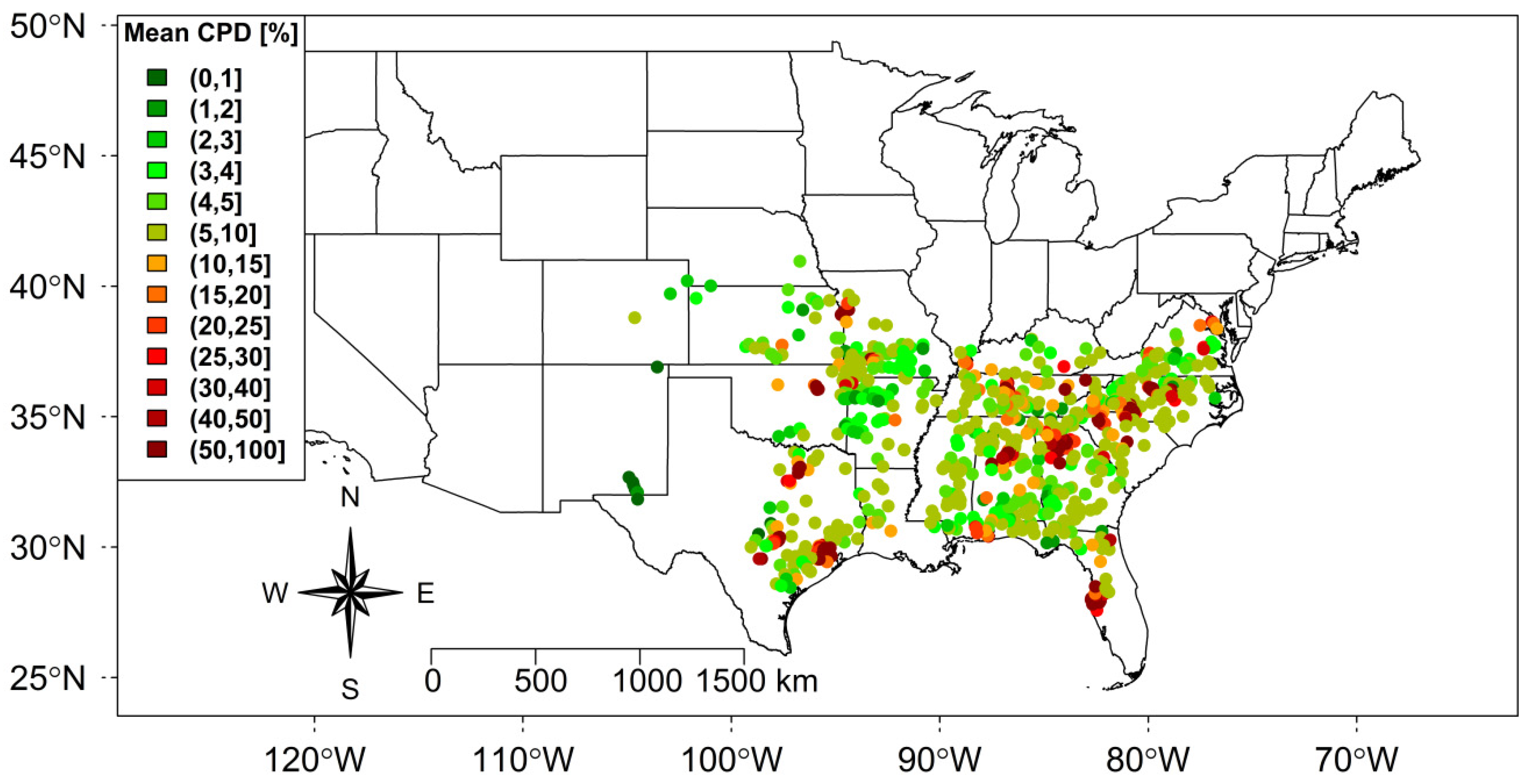
The sample of 2225 catchments was selected with respect to having limited snow effect, limited influence of dams and of storage facilities, and sufficiently available data, namely, at least 8 years with no gaps in hourly precipitations and potential evapotranspiration data and a rate of less than 30% hourly discharge gaps. Of the 2225 selected catchments, 870 are located in the United States (Figure 1) and the remaining 1355 are located in France (Figure 2). Their sizes range from 0.5 km2 to 110,000 km2, with a median value of 222 km2. Characterization in terms of urbanization was carried out using the Catchment Percent Developed (CPD) measure [54], which informs about the fraction of the catchment that is occupied by an urban landscape. Hence, CPD varies from 0% for a completely rural catchment to 100% for a completely urbanized catchment.
The U.S. catchments sample was selected among 9322 GAGE-II stream gauges maintained by the U.S. Geological Survey (USGS) [57]. Instantaneous flow measurement extraction was done by using the dataRetrieval package [58] in an R development environment [59]. The availability of hourly hydroclimatic time series was checked between 2002 and 2017. We used the National Land Cover Database (NLCD), available for the years 2001, 2006, and 2011 [60,61,62] to compute CPD as the percentage of urban pixels in the catchments, i.e., sum of classes 21 (developed: open space), 22 (developed: low intensity), 23 (developed: medium intensity), and 24 (developed: high intensity).
The French catchments sample was selected from the Banque Hydro database (http://www.hydro.eaufrance.fr) [63], where flow measurements are available for over 4000 stations across France. The availability of hourly streamflow and precipitation data was then checked for the period 1997–2012. CPD was computed using the CORINE Land Cover (CLC) product of the Copernicus Land Surface Monitoring Service available for the years 1990, 2000, 2006, and 2012 [64]. The classes considered to be urban were classes 11 (containing 111: continuous urban fabric, 112: discontinuous urban fabric) and 12 (containing 121: industrial or commercial units, 122: road and rail networks and associated land, 123: port areas, and 124: airports).
2.2. Catchment Descriptors
The catchment’s response is a function of two major drivers: climatic forcing and the landscape characteristics of the catchment. As resumed by Poncelet [65], the most relevant catchment descriptors can be binned into four categories:
- Climate: The catchment’s response inherits most of its variability from the catchment’s climate [66]. Many climate characteristics were computed over each catchment’s record period in order to limit their dependency on the record period. As climate descriptors, we considered mean hourly precipitations P (mm/h), mean hourly potential evapotranspiration PE (mm/h), humidity index HI (-), and flashiness of precipitations (-).
- Morphology: The catchment’s morphology is essential in predicting the catchment’s response timing and the repartition of precipitations into infiltration and runoff. For this reason, we used the catchment drained area (km2), drainage density (km/km2), and the median compound topographic index (-) as morphological descriptors.
- Land use: The catchment’s water yield and evapotranspiration losses depend on the catchment land use. Also, it is in our case of a central interest as we are dealing with the catchment’s level of urbanization. Thus, three land-use metrics were assessed: the CPD (%), the fraction of forest (%), and the fraction of open water (%).
- Geopedology: The catchment’s water transfers to and from the subjacent aquifers are modulated by the catchment’s geological and pedological characteristics. Hence, mean porosity (-), mean of log-transformed values of intrinsic permeability (m2), mean soil and subsoil content of gravel (%), silt (%), and clay (%) were considered as geopedological characteristics.
Note that some catchment descriptors were preliminary considered but found to be highly correlated with the aforementioned descriptors, such as flashiness of potential evapotranspiration (highly correlated with mean potential evapotranspiration), mean slope and mean elevation (highly anti-correlated with the compound topographic index), and mean soil and subsoil content of sand (highly anti-correlated with mean content of silt and clay). To avoid redundancy within each category of descriptors, we kept only the variables that did not exhibit high or significant correlation values with each other. This would prevent having an influenced variable importance by the presence of highly correlated variables. Table 1 provides a complete list of the descriptors, the computation method, and the data sources.
3. Methods
3.1. Model Parameters and Calibration
Representing the processes in an urbanized catchment requires working at sub-daily time steps since it is the timescale at which most of the urban hydrological processes are taking place [81,82]. Unfortunately, the fineness of the time step is limited by the availability of the hydroclimatic data that are needed for model forcing and validation. According to these two requirements, the hourly time step was chosen.
In this study, we used the GR4H lumped, conceptual hourly model [83,84] modified by Ficchi [85] to account for interception at sub-daily time steps. It was developed using large and worldwide samples of hydrological catchments over which it has achieved good performances in comparison with many other models [84,86]. In addition, its parsimonious structure helps understanding each parameter’s role in simulating the catchment’s response.
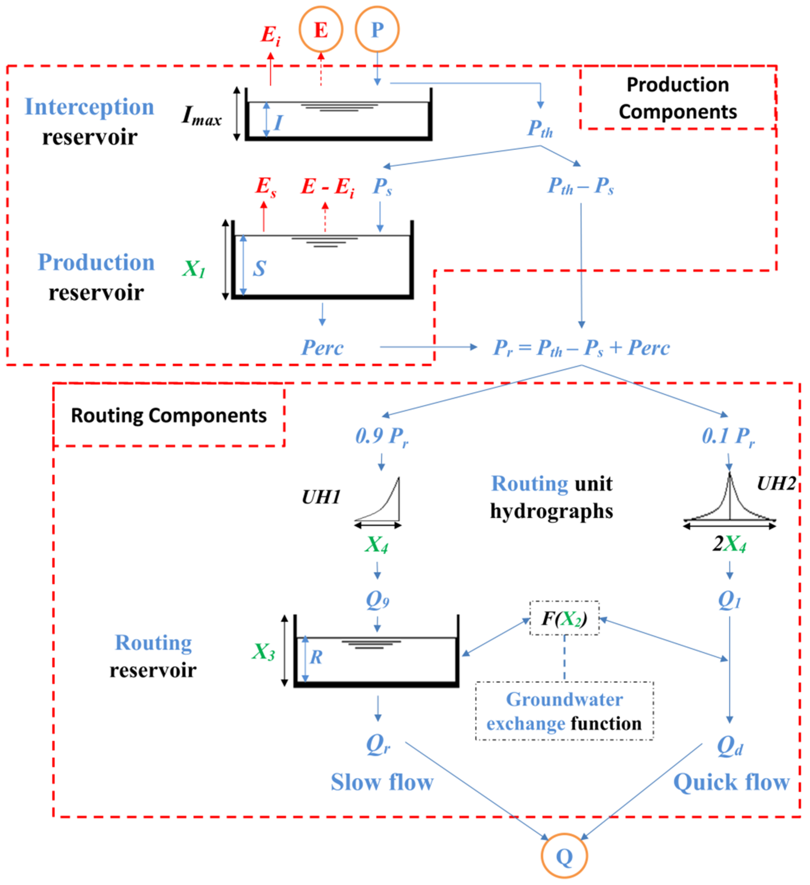
GR4H can be categorized as a soil moisture accounting model [56], which uses reservoir-style components and unit hydrographs to represent the following hydrological processes: interception, actual evapotranspiration, percolation from the soil, surface water–groundwater exchanges, quick and slow runoff. Figure 3 represents the model structure.
The model contains four free parameters. X1 (mm) is the production store maximum capacity. It controls the amount of water that can be stored and then lost either through actual evapotranspiration or percolation. X2 (mm/h) is the groundwater–surface water exchange rate, which is positive when importing water to the river stream and negative otherwise. X3 (mm) is the nonlinear routing store maximum capacity. It plays a role in determining the low-frequency component of the simulated hydrograph. X4 (h) controls the routing unit hydrograph time base. It represents the characteristic time of the catchment response. Ficchi [85] and Perrin et al. [56] give a more detailed description of the model equations.
The first year of the recorded period for each catchment was used for warm-up, and the model was then calibrated on the remaining years of the recorded period. The calibration procedure ran a local search algorithm including a steepest descent variable, as implemented by Edijatno et al. [87]. In order to account for possible dependency on the chosen objective function, the model calibration and evaluation were performed with respect to four different metrics: the Kling–Gupta efficiency (KGE) [88] and the Nash–Sutcliffe efficiency (NSE) [89] scores both applied on non-transformed (i.e., KGE and NSE) and square root values of observed and simulated runoffs (i.e., KGESR and NSESR). This was carried out using the airGR R package [90] in an R development environment [59].
3.2. Estimating the Model Parameters at Ungauged Locations Using RF
Following recent studies [43,49], we used the RF algorithm [33] for classification and prediction implemented in the randomForest R package [91] in an R development environment [59]. RF is a binning supervised ML algorithm that allows a large number of attributes (called predictors or independent variables) to be classified and used in order to carry out estimations of a response variable (called target variable or dependent variable) based on a large number of classification and regression trees (CARTs). As advocated by Breiman and Cutler [92] and presented by Tyralis et al. [30] in a review of recent literature, RF has the advantages of accuracy [93,94], efficiency in large databases [95], estimation of variable importance [93,94,96], and avoidance of overfitting [94].
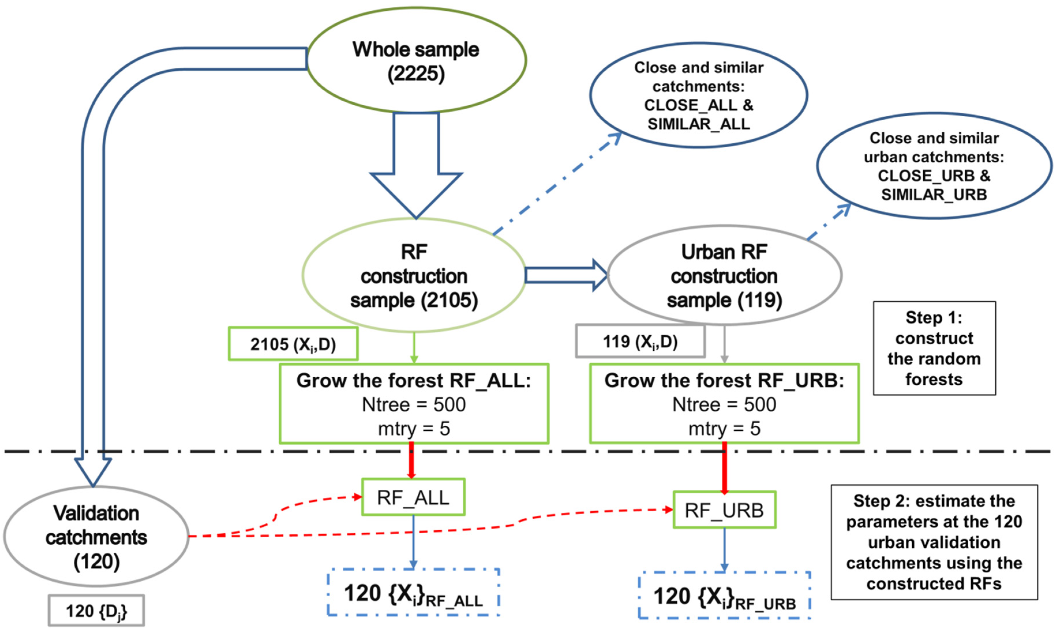
In this study, RF allowed to represent the multidimensional nonlinear relationships between each model parameter and the 15 catchment descriptors (Table 1). First, we divided the sample into two subsamples (Figure 4): the first one (120 catchments) served for validation of the regionalized model performance and was not used to train the RFs; it contained only urban catchments (CPD ≥ 20%). The second one (2105 catchments) was used to construct two RFs, i.e., as training samples: one with the whole subsample (RF_ALL, i.e., with rural and urban catchments) and another with only the urban catchments (RF_URB, i.e., with only 119 catchments that have a CPD over 20%). The idea was to see whether the RF can efficiently handle the large amount of training samples and produce equivalent model performances using both configurations. Second, the constructed RF was used to estimate model parameters {Xi} for the remaining 120 urban catchments (treated as ungauged) using their descriptors {Dj}. RF construction requires a specification about the number of trees to be grown (here Ntree = 500) and the number of variables to be selected randomly at each tree growing (here mtry was fixed at 5 by using the tuneRF function in the randomForest R package). While growing a tree, about one third of the cases—called out-of-bag (OOB) data—are left out of the sample [92,93], and then used to compute errors at each grown tree, e.g., the mean squared errors (MSE).
During the process of RF growing, we considered the IncMSE (%) metric to evaluate each descriptor importance in the RF-established relationships [43]. For a descriptor j (in our case j is between 1 and 15), the values were randomly permuted for the OOB data and a corresponding RF MSEj was determined. If MSE0 is the MSE of the RF computed during the construction, i.e., with non-permuted values for the OOB data, then IncMSE represents the difference between MSE0 and MSEj, after being computed and then scaled by the standard deviation of the differences over the trees. The greater the IncMSE, the more important the predictor variable.
3.3. Benchmark Regionalization Techniques
The validation sample (120 urban catchments) was used to set a benchmark for regionalization methods. For each catchment belonging to this sample, the recorded period was split into two subperiods P1 and P2. For each score SC (KGE, NSE, KGESR, and NSESR), calibration in P1 with respect to SC yielded a set of parameters to be controlled in P2 using the same evaluation criterion. We compared the control performances in P2 of this calibrated set with the performances of:
- The RF-estimated parameters using the catchment descriptors.
- The transferred parameters from the closest neighbor catchment. Spatial closeness was computed by weighting the distances between the catchment centroids (80%) and outlets (20%) [97]. Close catchments were selected either from the whole 2105 catchments used to train the RF_ALL (Figure 4) or from the 119 urban catchments used to grow RF_URB.
- The transferred parameters from the most similar catchment with respect to the descriptors used to construct the RF. For each descriptor, the catchment ranks were determined. Then, the Euclidean distance between ranks was computed in the hyperspace of descriptors [15]. Similar catchments were selected either from the whole 2105 catchments used to construct the RF_ALL (Figure 4) or from the 119 urban catchments used to construct RF_URB.
4. Results
4.1. Model Performances and Estimated Parameters
As explained before, two RFs were constructed in order to represent the relationships between calibrated model parameters and catchment descriptors. These calibrated model parameters were estimated over the whole period. They corresponded to relatively satisfactory scores at the hourly time step. The calibration median scores for the 2105 catchments were about 0.9 in terms of KGE and KGESR, 0.81 and 0.83 in terms of NSE and NSESR respectively. For the 119 urban catchments, a drop of performances was noticed, especially for median NSE (0.81 to 0.71), NSESR (0.83 to 0.77) and KGE (0.89 to 0.83), while the performances remained equivalent with regards to KGESR (0.9 to 0.87).
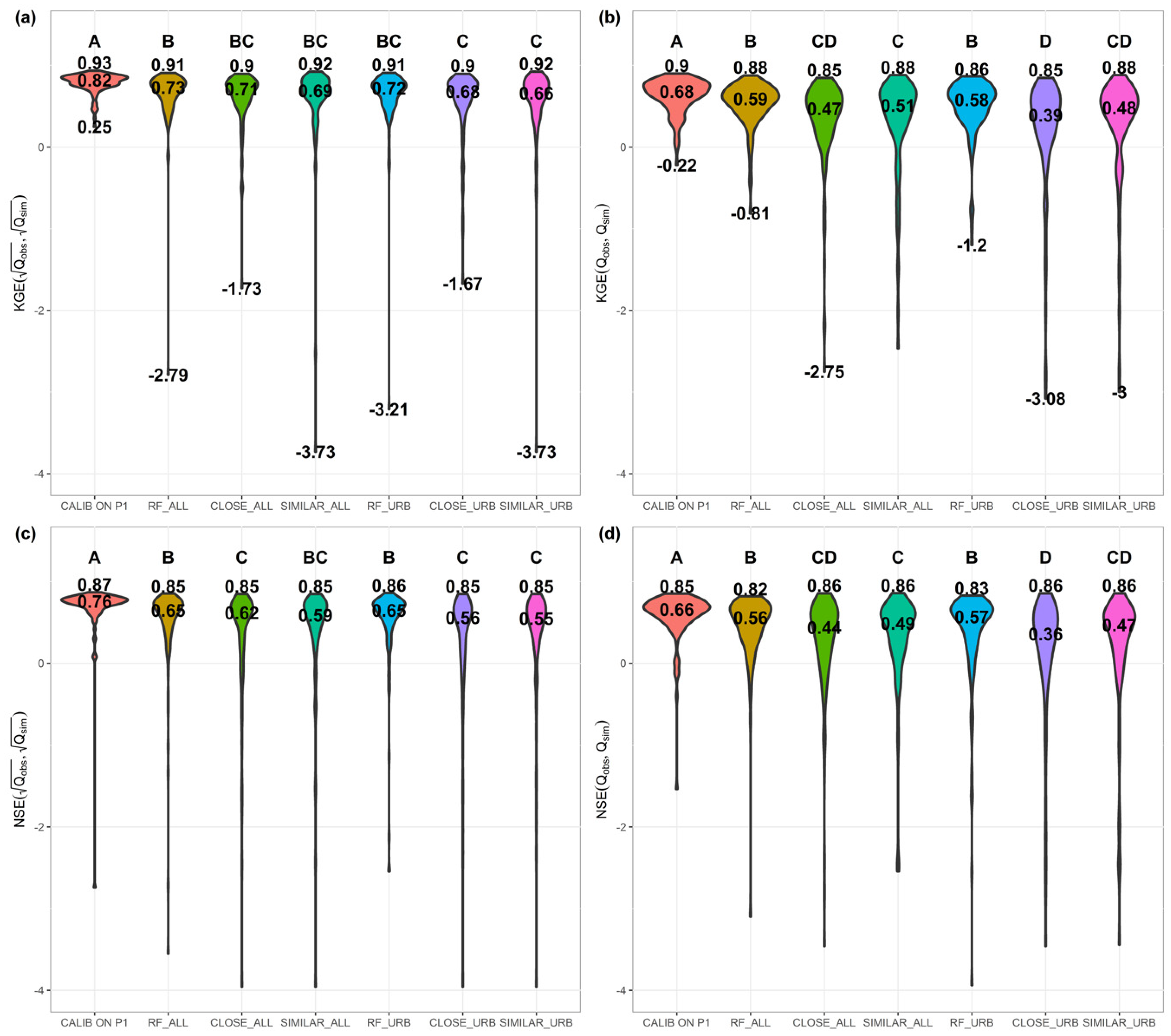
For every validation catchment, six sets of parameters were tested on the second period P2: Two sets were estimated from the RFs (RF_ALL and RF_URB) and four sets were transferred from the spatially close catchments (CLOSE_ALL and CLOSE_URB) and the similar catchments (SIMILAR_ALL and SIMILAR_URB). Their performances were then compared with the control scores of a calibrated set of parameters from P1. Figure 5 shows the distribution of the performances evaluated using each of the aforementioned metrics.
The RF-estimated parameters slightly but significantly (different distributions according to the statistical test, Figure 5) outperformed the benchmark regionalization methods based on spatial proximity or climate and landscape similarity. The differences were larger when using non-transformed flows. This was clearer when only urban catchments were considered for training; however, using only urbanized catchments for regionalization purposes reduced the model performance whatever the method considered, meaning that reducing the gauged catchment set is detrimental to regionalization, even if the reduction is designed to fit more the target ungauged catchments. Yet, the scores of time-transferred parameters (i.e., P1 to P2) remained unbeatable and significantly different (type A regardless of the considered metric).
If the performances of the RF-estimated parameters are significantly better than the transferred ones, how much do they succeed in resembling the calibrated parameters? Table 2 shows a comparison, by means of Spearman′s rank correlation, between the calibrated parameters using the four objective functions, and the estimated parameters from RF or from the transfer via spatial closeness or climate and landscape similarity using both the 2105-catchments sample and the 119-urban-catchments sample.
Except few cases, RF offered by far the best option in terms of parameter estimation for X1, X3, and X4, while for X2, none of the methods was satisfactory. Re-estimating the calibrated parameters with respect to transformed flows was systematically easier than when non-transformed flows were considered for calibration. The statistical test results indicated that the correlations were highly significant, even in the case of X2 where the values were hardly above 0.1. However, the R2 values were very moderate and in line with the values obtained in previous studies [10]. These values suggest that the calibrated parameters are difficult to estimate, meaning that there are still some remaining issues concerning the descriptors used and/or concerning model structure/parametrization uncertainties. Also, the clear superiority of the RF in estimating each parameter individually did not translate to model performances, especially in the case when KGESR and NSESR were considered. This may be due to the relative sensitivity of the model to its four free parameters and/or the fact that RF considers each parameter independently. Indeed, an RF was constructed for each model parameter, which means that the estimation is independent from one parameter to another. This might diminish the power of possible interactions between the parameters, i.e., compensation effects, whereas these effects were kept in the transferred sets.
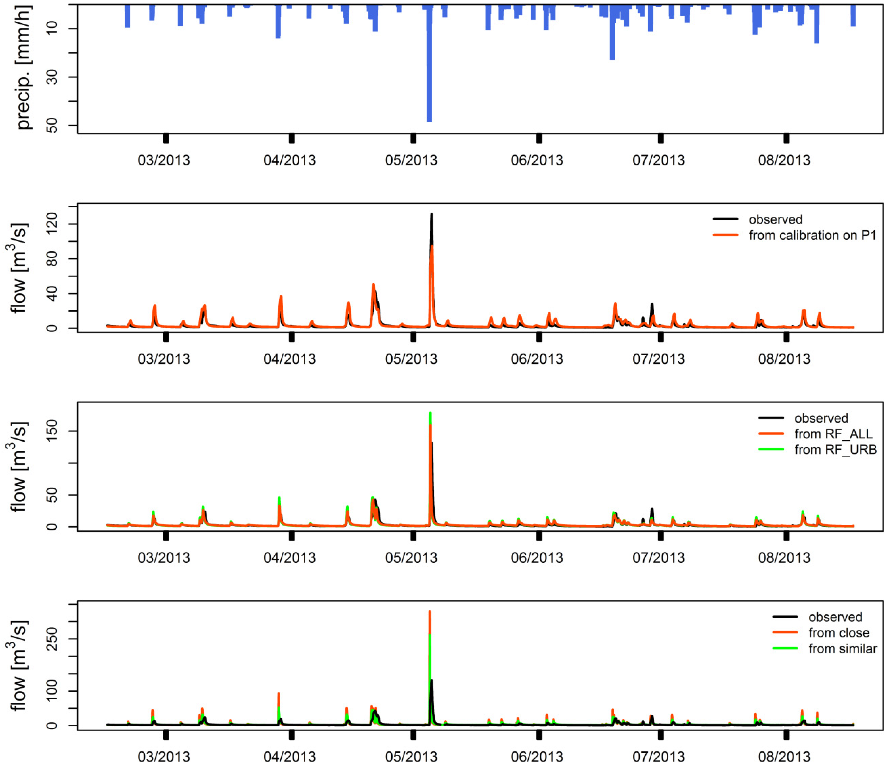
To illustrate the supremacy of the RF-estimated parameters, Figure 6 shows the simulated hydrographs for the Suwanee Creek catchment at Suwanee, Georgia (USGS code: 02334885, area: 122.1 km2, mean CPD: 59.6%) between 1 March 2013 and 31 August 2013. This period was chosen as it belongs to the catchment’s wettest year between 2010 and 2017 (i.e., P2). This catchment was recently investigated by Diem et al. [98] who found it to be hydrologically altered due to rapid shifts in the catchment’s land cover. For this example, only the case when KGESR was used is shown. Table 3 details the values of the five sets of parameters used to compute these hydrographs: estimated from RF_ALL and RF_URB, transferred from calibration over the catchment’s first period P1, and transferred from the closest catchment (Dick Creek at Old Atlanta Road, near Suwanee, Georgia, USGS code: 02334620, area: 17.8 km2, mean CPD: 55.3%) and the most similar catchment (Reedy River near Greenville, South Carolina, USGS code: 02164000, area: 125.1 km2, mean CPD: 68.2%).
We can see that the transferred parameters from P1 and the RF-estimated parameters are the best ones to succeed in reproducing the observed flow. In this particular period, a heavy rainfall event was recorded during the second half of May, which attained a maximum intensity of 48.5 mm/h. The corresponding observed peak flow was slightly underestimated by the time-transferred parameters, slightly overestimated by the RF-estimated parameters but erroneously overestimated by the transferred parameters from the closest or the most similar catchment (Table 3).
4.2. Descriptor Importance
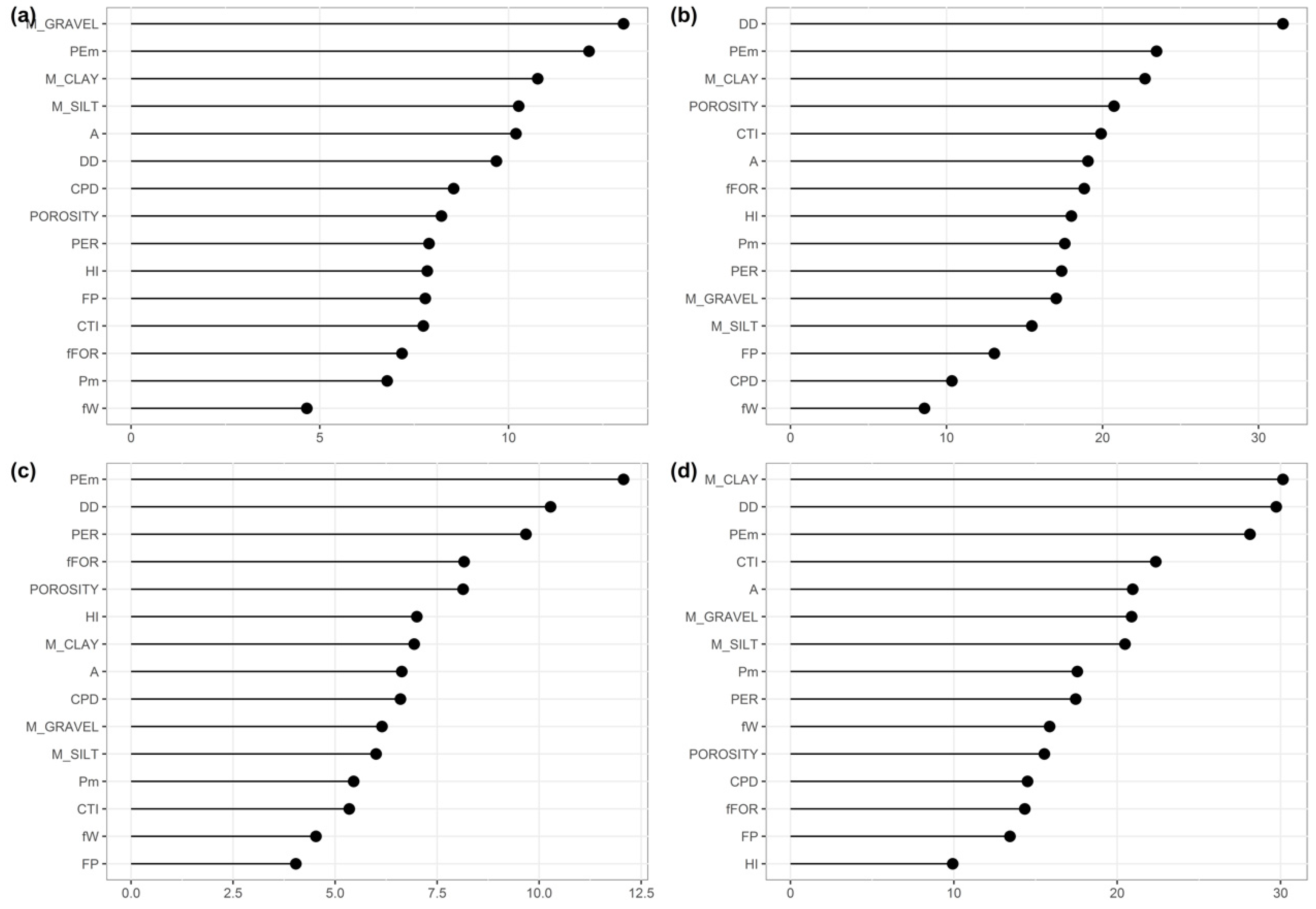
As mentioned earlier, the importance of descriptors in determining each parameter was measured using IncMSE (%), for which the most important variables exhibited the highest scores. The objective was to see which descriptors weighed the most in the regression relationships, and how powerful the CPD measure was in deciding the parameter values vis-à-vis the other descriptors. As RF_ALL and RF_URB performed similarly, we retained for the analysis the RF_ALL approach only, since it integrates the largest amount of information and the widest panel of situations. Also, we constrained the analysis to the trained RF_ALL using estimated parameters with respect to KGESR, as the ranks were not significantly different from one objective function to another, especially the top ranks. Figure 7 shows the importance of the descriptors for each parameter in terms of IncMSE (%).
Soil characteristics (mean content of gravel, silt, and clay) and mean potential evapotranspiration exhibited the highest importance scores in determining X1. Land-use characteristics, in particular CPD, also exhibited moderate weights in deciding X1. However, they were not highly decisive compared with the remaining descriptors. This seems coherent, as X1 modulates the soil–atmosphere interactions, thus relying on a large number of descriptors. In the case of X2, the drainage density yielded a remarkable score, followed by mean potential evapotranspiration PEm and some soil characteristics (mean content of clay, mean porosity) and other morphology descriptors (area and CTI). The influence of PEm on X2 may stem from the possible interaction with X1, as both play a role in matching the catchment water budget. The drainage density, the mean content of clay, the porosity, and CTI give implicit or explicit information about the soil permeability, hence, their influence over X2 was expected as X2 characterizes the interactions between the groundwater and the surface water. For X3 and X4, the most influential descriptors were very easily distinguishable. PEm had the heaviest weight on X3, the parameter that shapes the component of slow flow; this may be due to the fact that in recession periods, PEm plays a major role in conditioning the recession flow curvature. The mean content of clay, PEm, and the drainage density played a major role in determining X4. This parameter is coherent with the characteristic time of the catchment response, and drives majorly the correlation at the hourly time step between the observed and simulated flows. Besides, X4 is correlated with the catchment area, which was revealed to be the fifth most influential descriptor.
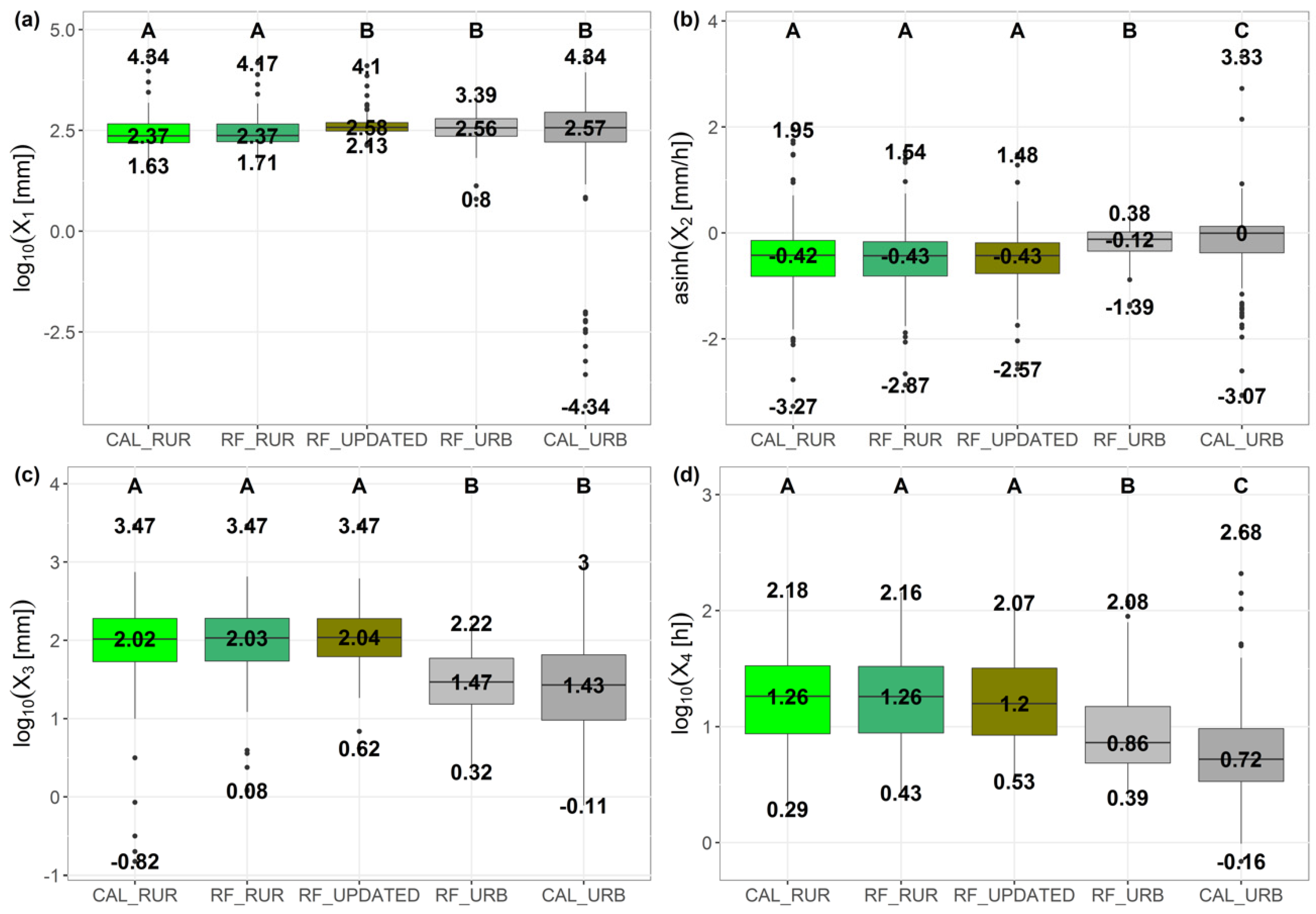
The sole measure of urbanization was not found to be useful in determining the calibrated model parameters compared with other descriptors, where it was at best ranked as 7th out of 15. Therefore, we studied whether the constructed RF was sensitive to this measure. We randomly selected 120 rural catchments from the 2105-catchments sample by applying a CPD maximum threshold of 5%. Each rural catchment was then matched with one of the 120-urban-catchments validation sample. We subsequently estimated two sets of parameters for each rural catchment: one without altering the catchment characteristics (RUR) and the other by replacing the rural catchment CPD by the CPD of the corresponding urban catchment. These two sets were then compared with the calibrated rural parameters, the calibrated urban parameters, and the RF-estimated parameters of the 120-urban-catchments sample. The tests were conducted using the four objective functions, but only the results corresponding to KGESR are discussed hereafter. Figure 8 shows the distribution of the parameters.
At first, the sets of calibrated parameters were different between the rural and the urban samples. The main impacts were observed on X3 and X4, which represents the transfer function of the model. Their values were lower for the urban catchments, meaning that the time response of the catchments was relatively shortened. The results of the Mann–Whitney–Wilcoxon (MWW) statistical equality test indicated that there were also differences in the budget parameters, i.e., X1 and X2.
The RF_RUR and CAL_RUR presented similar distributions to RF_URB and CAL_URB (X1 and X3), meaning that the RF approach succeeded in adapting the model parameters depending on the urbanization stage, if the training sample was adapted to the target catchments. Exceptions were made for X2 and X4, where the statistical test results indicated that RF-estimated parameters for the urban catchments were different from the calibrated ones. For these two parameters, CPD had the lowest ranks (12th and 14th out of 15), which means that for urban catchments with relatively low CPD values (i.e., close to 20%), the estimation of these two parameters was driven more by other descriptors than by CPD.
The shifts in CPD over the rural catchments were between +15.7% and +98.3%, with a median shift of +59.4%. However, none of the parameters responds to this shift, except for parameter X1 where the parameters exhibited a trend toward higher values as witnessed in the urban sample (confirmed by the MWW test), which suggests an overall weak CPD sensitivity of the RF_ALL.
5. Discussion and Conclusions
5.1. Regionalization with RF: What Is Appreciated and What Is Depreciated?
In this case study, we used the RF algorithm to represent the nonlinear relationships between calibrated model parameters and catchment descriptors. Our goal was to estimate these parameters at (assumed) ungauged intensively urbanized catchments, either by giving exhaustive information about a large number of training catchments or by restraining the focus to urban catchments only. In a regionalization framework, the problem was treated via a priori parameter estimation. A comparison was made with transfer-based regionalization approaches. Besides, the study was performed using a large sample of catchments at hourly time steps, which represents two features of originality of this work.
With regards to the chosen spatial representation, the very heterogeneous aspect of urban catchments’ landscape requires using distributed approaches, since the spatial configuration of the rural and urban surfaces can intensify or mitigate the impact of the urban surfaces on the catchment’s response [81,82,99,100]. However, it could have added more parameters in comparison with the lumped approach adopted herein, and which we believe that is somehow sufficient for our regionalization objectives, by keeping a number of parameters that are more easily interpreted. Moreover, space is left for efforts to convey this heterogeneity up to the catchment scale from finer scales, via hydrologically relevant landscape descriptors [54,55,101].
Concerning the regionalized model simulations, the results showed a relatively good performance of the RF for parameter estimation (Figure 5). The supremacy of the RF algorithm over the transfer-based regionalization methods was not sensitive to the chosen evaluation metric, and it was clearer when using non-transformed flows in calibration and evaluation. Moreover, the results were not altered by the size of the construction data, which confirms the robustness of the algorithm. Also, RF demonstrated better performance compared with transfer-based regionalization methods with regards to parameter estimation (Table 2).
The loss in the regionalized model performance compared with the time-transferred parameters remained large and comparable to previous regionalization studies with large-sample experiments. This can be explained by (1) the fact that the calibrated parameters were not easily estimable, since they may only represent a numerical optimum, although they were estimated over the entire recorded period (from 8 to 16 years at the hourly time step) in order to guarantee a maximum of stability. Note that the RFs are incapable of producing predictions outside the training range, as mentioned by Tyralis et al. [30] and Hengl et al. [102]. Furthermore, the effects of compensation were not handled efficiently and (2) part of the difficulty might lie behind the fineness of the time step at which the study was performed. Regionalization at an hourly time step is rare [103] or even nonexistent in comparison with daily and monthly time steps [104]. If the water budget estimation at hourly time steps is as difficult as at daily time steps, then the challenge is to guarantee good correlation scores (i.e., synchronization) between the observed and the simulated streamflows, i.e., good estimation of the routing parameters. With regard to X3 and X4, RF_ALL had a moderate maximum score in estimating X3 (R2 = 0.45, objective function: KGESR, Table 2) but failed to maintain the same score for X4 (R2 = 0.29, Table 2), and when the estimation of X4 was satisfactory (R2 = 0.61, objective function: NSE, Table 2), the corresponding X3 estimation score was low (R2 = 0.32, Table 2). RF_URB appeared to be globally more efficient in estimating these routing parameters (R2 = 0.41–0.6 for X4), perhaps due to the homogeneity in catchment size between the two urban-catchments samples; knowing that X4 is, to first order, dependent on the catchment area, (3) the descriptors might not be relevant in regionalizing the model parameters, or the methods of their determination were not suitable. For the time scale, the descriptors were averaged over the whole simulation period, and also aggregated spatially up to the catchment scale, under the assumption of stable catchment characteristics over the study period. Intra-temporal and intra-catchment variability representation could yield more information to explain the variance of the parameters.
RF allows one to assess variable importance. However, interpreting the relative importance of the descriptors was not straightforward owing to (1) the integrative nature of both the parameters and descriptors and (2) their inter-correlations. Generally, the interpretability of the RF algorithm is not as obvious as its skillfulness [30,105,106], which makes it an efficient prediction algorithm but an arduously interpretable one.
5.2. Weak Sensitivity of the RF-Derived Relationships with the Urbanization Measure
Since the variable importance results showed non-significant scores for CPD, we attempted to examine whether shifts in this measure would have an impact on the parameter values.
As can be seen in Figure 8, X1 was the only parameter that responded to the CPD shifts, displaying values similar to the ones estimated for the urban catchments. The reasons why this shift was not visible on the remaining parameters could be (1) the insensitivity of the model parameters to the CPD measure and (2) the multidimensional aspect of the parameter–descriptor relationship, which makes the parameters less sensitive to one descriptor itself but wholly dependent on all the descriptors, as shown in the variable importance, where almost no variable was remarkably influential. Perhaps this parameter insensitivity was amplified by the rural catchment insensitivity to the CPD shifts, as the natural descriptors (i.e., all the descriptors except CPD) predominate, and (3) the unsuitability (or insufficiency) of the CPD measure to describe the urbanization features, which may be viewed as a need for other urbanization descriptors to be included.
5.3. Conclusions and Perspectives
As the ML algorithms are increasingly applied for various purposes in hydrology, we aimed at exploring the capacity of the RF algorithm in regionalizing hourly hydrological model parameters. The RF algorithm was applied using a large sample of American and French catchments, for which several climate and landscape descriptors were estimated. Two RFs were constructed for different sizes of training samples of catchments. The objective was to represent the relationships between the calibrated model parameters and climate/landscape descriptors and then use these relationships to carry out estimates on urban catchments. The RF permitted us to: (1) achieve relatively good regionalized model performances compared with transfer-based regionalization methods, regardless of the construction sample size or the calibration objective function; (2) attain good performances concerning the model parameter estimations, but even better with regard to the transferring methods; and (3) perceive how increasing rates of urbanization influence model parameters. This large-sample hourly regionalization work at ungauged urban catchments has confirmed the need for ML algorithms such as RF in treating high-dimensional problems, uncovering nonlinear functions and, accounting for the uncertainty in parameter prediction (not discussed in this paper) with high efficiency and robustness.
Looking ahead, the sets of targeted parameter values should be refined more by looking for multi-objective suitable sets or even generic ones [21,107]. Moreover, other urbanization descriptors should be included in order to refine the relationships. Compensation effects should be handled by estimating all the parameters at once using a unique RF for all the parameters or an iterative procedure where the sets of parameters are considered to be dependent on each other.
Author Contributions
Conceptualization, M.S., L.O. and P.R.; Investigation and software, M.S. and L.O.; Formal analysis, M.S., L.O. and P.R.; Funding acquisition, project administration and supervision, L.O. and P.R.; Methodology, M.S., L.O. and P.R.; Writing – original draft, M.S.; Writing – review & editing, M.S., L.O. and P.R.
Funding
This research received no external funding.
Acknowledgments
This study utilized data from several sources. For the U.S. catchments, instantaneous streamflow data were collected from the USGS website (available at http://waterdata.usgs.gov/) using the dataRetrieval R package. Hourly rainfall data were extracted from the NEXRAD Stage IV archive (available at https://data.eol.ucar.edu/dataset/21.093) using the geoknife R package. Daily temperature data were extracted from the Daymet dataset (available at https://daymet.ornl.gov/). Geospatial data and classifications for stream gages maintained by the U.S. Geological Survey (USGS) called Gages II are available at http://water.usgs.gov/lookup/getspatial?gagesII_Sept2011. National Land Cover Database (NLCD) data were obtained from the Multi-Resolution Land Characteristics (MRLC) Consortium website (available at http://www.mrlc.gov/about.php). Hydrographic networks were extracted from the NHD dataset (available at https://www.usgs.gov/core-science-systems/ngp/national-hydrography) using the FedData R package. For the French catchments, flow measurements were extracted from Banque Hydro (available at http://www.hydro.eaufrance.fr/). Hourly rainfall data were extracted from the COMEPHORE product obtained from Meteo-France. Hourly temperature data were extracted from the SAFRAN product obtained from Meteo-France. CORINE Land Cover (CLC) data were obtained from the Copernicus Land Monitoring Service website (https://land.copernicus.eu/pan-european/corine-land-cover). The hydrographic networks were extracted from the BD Carthage® product provided by the IGN (http://professionnels.ign.fr/bdcarthage). Soil properties were described using the GLHYMPS dataset (available at http://www.groundwaterscienceandsustainability.org/data.html) and the HWSD dataset extracted using the hwsd R package. Finally, we thank Jordan Read (USGS), David Blodgett (USGS), David Watkins (USGS), and William Watkins (USGS) for their help concerning the geoknife R package, Tammy Walker (ORNL) and Michele Thornton (ORNL) for their help about the Daymet dataset.
Conflicts of Interest
The authors declare no conflict of interest.
References
- Beven, K. How far can we go in distributed hydrological modelling? Hydrol. Earth Syst. Sci. 2001, 5, 1–12. [Google Scholar] [CrossRef]
- Klemeš, V. Operational testing of hydrological simulation models. Hydrol. Sci. J. 1986, 31, 13–24. [Google Scholar] [CrossRef]
- Beven, K. Beyond the Primer: Predictions in Ungauged Basins. In Rainfall-Runoff Modelling: The Primer; Wiley-Blackwell: Chichester, UK, 2012; pp. 329–342. ISBN 978-0-470-71459-1. [Google Scholar]
- Sivapalan, M.; Takeuchi, K.; Franks, S.W.; Gupta, V.K.; Karambiri, H.; Lakshmi, V.; Liang, X.; McDonnell, J.J.; Mendiondo, E.M.; O’Connell, P.E.; et al. IAHS Decade on Predictions in Ungauged Basins (PUB), 2003–2012: Shaping an exciting future for the hydrological sciences. Hydrol. Sci. J. 2003, 48, 857–880. [Google Scholar] [CrossRef]
- Duan, Q.; Schaake, J.; Andréassian, V.; Franks, S.; Goteti, G.; Gupta, H.V.; Gusev, Y.M.; Habets, F.; Hall, A.; Hay, L.; et al. Model Parameter Estimation Experiment (MOPEX): An overview of science strategy and major results from the second and third workshops. J. Hydrol. 2006, 320, 3–17. [Google Scholar] [CrossRef] [Green Version]
- Hrachowitz, M.; Savenije, H.H.G.; Blöschl, G.; McDonnell, J.J.; Sivapalan, M.; Pomeroy, J.W.; Arheimer, B.; Blume, T.; Clark, M.P.; Ehret, U.; et al. A decade of Predictions in Ungauged Basins (PUB)—A review. Hydrol. Sci. J. 2013, 58, 1198–1255. [Google Scholar] [CrossRef]
- Seibert, J. Regionalisation of parameters for a conceptual rainfall-runoff model. Agric. For. Meteorol. 1999, 98, 279–293. [Google Scholar] [CrossRef]
- Sefton, C.E.M.; Howarth, S.M. Relationships between dynamic response characteristics and physical descriptors of catchments in England and Wales. J. Hydrol. 1998, 211, 1–16. [Google Scholar] [CrossRef]
- Drogue, G.; Leviandier, T.; Pfister, L.; Idrissi, A.E.; Iffly, J.-F.; Hoffmann, L.; Guex, F.; Hingray, B.; Humbert, J. The applicability of a parsimonious model for local and regional prediction of runoff. Hydrol. Sci. J. 2002, 47, 905–920. [Google Scholar] [CrossRef]
- Merz, R.; Blöschl, G. Regionalisation of catchment model parameters. J. Hydrol. 2004, 287, 95–123. [Google Scholar] [CrossRef] [Green Version]
- Oudin, L.; Andréassian, V.; Loumagne, C.; Michel, C. How informative is land-cover for the regionalization of the GR4J rainfall-runoff model? Lessons of a downward approach. IAHS Publ. 2006, 307, 246–255. [Google Scholar]
- Anderson, R.M.; Koren, V.I.; Reed, S.M. Using SSURGO data to improve Sacramento Model a priori parameter estimates. J. Hydrol. 2006, 320, 103–116. [Google Scholar] [CrossRef]
- Boughton, W.; Chiew, F. Estimating runoff in ungauged catchments from rainfall, PET and the AWBM model. Environ. Model. Softw. 2007, 22, 476–487. [Google Scholar] [CrossRef] [Green Version]
- Hundecha, Y.; Ouarda, T.B.M.J.; Bárdossy, A. Regional estimation of parameters of a rainfall-runoff model at ungauged watersheds using the “spatial” structures of the parameters within a canonical physiographic-climatic space. Water Resour. Res. 2008, 44. [Google Scholar] [CrossRef]
- Oudin, L.; Andréassian, V.; Perrin, C.; Michel, C.; Le Moine, N. Spatial proximity, physical similarity, regression and ungaged catchments: A comparison of regionalization approaches based on 913 French catchments. Water Resour. Res. 2008, 44. [Google Scholar] [CrossRef]
- Samaniego, L.; Kumar, R.; Attinger, S. Multiscale parameter regionalization of a grid-based hydrologic model at the mesoscale. Water Resour. Res. 2010, 46. [Google Scholar] [CrossRef] [Green Version]
- Vandewiele, G.L.; Elias, A. Monthly water balance of ungauged catchments obtained by geographical regionalization. J. Hydrol. 1995, 170, 277–291. [Google Scholar] [CrossRef]
- Parajka, J.; Merz, R.; Blöschl, G. A comparison of regionalisation methods for catchment model parameters. Hydrol. Earth Syst. Sci. 2005, 9, 157–171. [Google Scholar] [CrossRef] [Green Version]
- Kim, U.; Kaluarachchi, J.J. Application of parameter estimation and regionalization methodologies to ungauged basins of the Upper Blue Nile River Basin, Ethiopia. J. Hydrol. 2008, 362, 39–56. [Google Scholar] [CrossRef]
- Oudin, L.; Kay, A.; Andréassian, V.; Perrin, C. Are seemingly physically similar catchments truly hydrologically similar? Water Resour. Res. 2010, 46. [Google Scholar] [CrossRef]
- Andréassian, V.; Le Moine, N.; Perrin, C.; Ramos, M.-H.; Oudin, L.; Mathevet, T.; Lerat, J.; Berthet, L. All that glitters is not gold: the case of calibrating hydrological models: Invited Commentary. Hydrol. Process. 2012, 26, 2206–2210. [Google Scholar] [CrossRef]
- Fernandez, W.; Vogel, R.M.; Sankarasubramanian, A. Regional calibration of a watershed model. Hydrol. Sci. J. 2000, 45, 689–707. [Google Scholar] [CrossRef]
- Parajka, J.; Blöschl, G.; Merz, R. Regional calibration of catchment models: Potential for ungauged catchments. Water Resour. Res. 2007, 43. [Google Scholar] [CrossRef]
- Castiglioni, S.; Lombardi, L.; Toth, E.; Castellarin, A.; Montanari, A. Calibration of rainfall-runoff models in ungauged basins: A regional maximum likelihood approach. Adv. Water Resour. 2010, 33, 1235–1242. [Google Scholar] [CrossRef]
- Bourgin, F.; Andréassian, V.; Perrin, C.; Oudin, L. Transferring global uncertainty estimates from gauged to ungauged catchments. Hydrol. Earth Syst. Sci. 2015, 19, 2535–2546. [Google Scholar] [CrossRef]
- Olden, J.D.; Poff, N.L. Redundancy and the choice of hydrologic indices for characterizing streamflow regimes. River Res. Appl. 2003, 19, 101–121. [Google Scholar] [CrossRef]
- Yadav, M.; Wagener, T.; Gupta, H. Regionalization of constraints on expected watershed response behavior for improved predictions in ungauged basins. Adv. Water Resour. 2007, 30, 1756–1774. [Google Scholar] [CrossRef]
- Zhang, Z.; Wagener, T.; Reed, P.; Bhushan, R. Reducing uncertainty in predictions in ungauged basins by combining hydrologic indices regionalization and multiobjective optimization. Water Resour. Res. 2008, 44. [Google Scholar] [CrossRef]
- Shen, C. A Transdisciplinary Review of Deep Learning Research and Its Relevance for Water Resources Scientists. Water Resour. Res. 2018, 54, 8558–8593. [Google Scholar] [CrossRef]
- Tyralis, H.; Papacharalampous, G.; Langousis, A. A Brief Review of Random Forests for Water Scientists and Practitioners and Their Recent History in Water Resources. Water 2019, 11, 910. [Google Scholar] [CrossRef]
- Merz, R.; Blöschl, G.; Parajka, J.D. Regionalization methods in rainfall-runoff modelling using large catchment samples. IAHS Publ. 2006, 307, 117–125. [Google Scholar]
- Carbajal, J.P.; Bellos, V. An Overview of the Role of Machine Learning in Hydraulic and Hydrological Modeling. Available online: engrxiv.org/wgm72 (accessed on 25 April 2019).
- Breiman, L. Random Forests. Mach. Learn. 2001, 45, 5–32. [Google Scholar] [CrossRef] [Green Version]
- Liakos, K.G.; Busato, P.; Moshou, D.; Pearson, S.; Bochtis, D. Machine Learning in Agriculture: A Review. Sensors 2018, 18, 2674. [Google Scholar] [CrossRef] [PubMed]
- Cutler, D.R.; Edwards, T.C.; Beard, K.H.; Cutler, A.; Hess, K.T.; Gibson, J.; Lawler, J.J. Random Forests for Classification in Ecology. Ecology 2007, 88, 2783–2792. [Google Scholar] [CrossRef] [PubMed]
- Gislason, P.O.; Benediktsson, J.A.; Sveinsson, J.R. Random Forests for land cover classification. Pattern Recognit. Lett. 2006, 27, 294–300. [Google Scholar] [CrossRef]
- Diez-Sierra, J.; del Jesus, M. Subdaily Rainfall Estimation through Daily Rainfall Downscaling Using Random Forests in Spain. Water 2019, 11, 125. [Google Scholar] [CrossRef]
- He, X.; Chaney, N.W.; Schleiss, M.; Sheffield, J. Spatial downscaling of precipitation using adaptable random forests. Water Resour. Res. 2016, 52, 8217–8237. [Google Scholar] [CrossRef]
- Muñoz, P.; Orellana-Alvear, J.; Willems, P.; Célleri, R. Flash-Flood Forecasting in an Andean Mountain Catchment—Development of a Step-Wise Methodology Based on the Random Forest Algorithm. Water 2018, 10, 1519. [Google Scholar] [CrossRef]
- Sultana, Z.; Sieg, T.; Kellermann, P.; Müller, M.; Kreibich, H. Assessment of Business Interruption of Flood-Affected Companies Using Random Forests. Water 2018, 10, 1049. [Google Scholar] [CrossRef]
- Wang, Z.; Lai, C.; Chen, X.; Yang, B.; Zhao, S.; Bai, X. Flood hazard risk assessment model based on random forest. J. Hydrol. 2015, 527, 1130–1141. [Google Scholar] [CrossRef]
- Buchanan, B.; Auerbach, D.A.; Knighton, J.; Evensen, D.; Fuka, D.R.; Easton, Z.; Wieczorek, M.; Archibald, J.A.; McWilliams, B.; Walter, T. Estimating dominant runoff modes across the conterminous United States. Hydrol. Process. 2018, 32, 3881–3890. [Google Scholar] [CrossRef]
- Addor, N.; Nearing, G.; Prieto, C.; Newman, A.J.; Le Vine, N.; Clark, M.P. A Ranking of Hydrological Signatures Based on Their Predictability in Space. Water Resour. Res. 2018, 54, 8792–8812. [Google Scholar] [CrossRef]
- Booker, D.J.; Woods, R.A. Comparing and combining physically-based and empirically-based approaches for estimating the hydrology of ungauged catchments. J. Hydrol. 2014, 508, 227–239. [Google Scholar] [CrossRef] [Green Version]
- Carlisle, D.M.; Falcone, J.; Wolock, D.M.; Meador, M.R.; Norris, R.H. Predicting the natural flow regime: Models for assessing hydrological alteration in streams. River Res. Appl. 2010, 26, 118–136. [Google Scholar] [CrossRef]
- Snelder, T.H.; Lamouroux, N.; Leathwick, J.R.; Pella, H.; Sauquet, E.; Shankar, U. Predictive mapping of the natural flow regimes of France. J. Hydrol. 2009, 373, 57–67. [Google Scholar] [CrossRef]
- Brunner, M.I.; Seibert, J.; Favre, A.-C. Representative sets of design hydrographs for ungauged catchments: A regional approach using probabilistic region memberships. Adv. Water Resour. 2018, 112, 235–244. [Google Scholar] [CrossRef]
- Prieto, C.; Vine, N.L.; Kavetski, D.; Garcia, E.; Medina, R. Flow prediction in ungauged catchments using probabilistic Random Forests regionalization and new statistical adequacy tests. Water Resour. Res. 2019, 55, 4364–4392. [Google Scholar] [CrossRef]
- Zhang, Y.; Chiew, F.H.S.; Li, M.; Post, D. Predicting Runoff Signatures Using Regression and Hydrological Modeling Approaches. Water Resour. Res. 2018, 54, 7859–7878. [Google Scholar] [CrossRef]
- Boulesteix, A.-L.; Janitza, S.; Kruppa, J.; König, I.R. Overview of random forest methodology and practical guidance with emphasis on computational biology and bioinformatics. Wiley Interdiscip. Rev. Data Min. Knowl. Discov. 2012, 2, 493–507. [Google Scholar] [CrossRef] [Green Version]
- Cheng, S.; Lee, C.; Lee, J. Effects of Urbanization Factors on Model Parameters. Water Resour. Manag. 2010, 24, 775–794. [Google Scholar] [CrossRef]
- Chen, R.; Chuang, W.-N.; Cheng, S. Effects of urbanization variables on model parameters for watershed divisions. Hydrol. Sci. J. 2014, 59, 1167–1183. [Google Scholar] [CrossRef]
- Kjeldsen, T.R.; Miller, J.D.; Packman, J.C. Modelling design flood hydrographs in catchments with mixed urban and rural land cover. Hydrol. Res. 2013, 44, 1040–1057. [Google Scholar] [CrossRef]
- Oudin, L.; Salavati, B.; Furusho-Percot, C.; Ribstein, P.; Saadi, M. Hydrological impacts of urbanization at the catchment scale. J. Hydrol. 2018, 559, 774–786. [Google Scholar] [CrossRef] [Green Version]
- Salavati, B.; Oudin, L.; Furusho-Percot, C.; Ribstein, P. Modeling approaches to detect land-use changes: Urbanization analyzed on a set of 43 US catchments. J. Hydrol. 2016, 538, 138–151. [Google Scholar] [CrossRef] [Green Version]
- Perrin, C.; Michel, C.; Andréassian, V. Improvement of a parsimonious model for streamflow simulation. J. Hydrol. 2003, 279, 275–289. [Google Scholar] [CrossRef]
- Falcone, J.A. GAGES-II: Geospatial Attributes of Gages for Evaluating Streamflow; US Geological Survey: Reston, VA, USA, 2011.
- Hirsch, R.M.; Cicco, L.A.D. User guide to Exploration and Graphics for RivEr Trends (EGRET) and dataRetrieval: R packages for hydrologic data. In Techniques and Methods; U.S. Geological Survey: Reston, VA, USA, 2015. [Google Scholar]
- R Core Team. R: A Language and Environment for Statistical Computing; R Foundation for Statistical Computing: Vienna, Austria, 2017. [Google Scholar]
- Homer, C.; Huang, C.; Yang, L.; Wylie, B.; Coan, M. Development of a 2001 national land-cover database for the United States. Photogramm. Eng. Remote Sens. 2004, 70, 829–840. [Google Scholar] [CrossRef]
- Homer, C.; Dewitz, J.; Fry, J.; Coan, M.; Hossain, N.; Larson, C.; Herold, N.; McKerrow, A.; VanDriel, J.N.; Wickham, J. Completion of the 2001 national land cover database for the counterminous United States. Photogramm. Eng. Remote Sens. 2007, 73, 337–341. [Google Scholar]
- Homer, C.; Dewitz, J.; Yang, L.; Jin, S.; Danielson, P.; Xian, G.; Coulston, J.; Herold, N.; Wickham, J.; Megown, K. Completion of the 2011 National Land Cover Database for the conterminous United States–Representing a decade of land cover change information. Photogramm. Eng. Remote Sens. 2015, 81, 345–354. [Google Scholar]
- Leleu, I.; Tonnelier, I.; Puechberty, R.; Gouin, P.; Viquendi, I.; Cobos, L.; Foray, A.; Baillon, M.; Ndima, P.-O. La refonte du système d’information national pour la gestion et la mise à disposition des données hydrométriques. Houille Blanche 2014, 25–32. [Google Scholar] [CrossRef]
- Büttner, G.; Kosztra, B.; Maucha, G.; Pataki, R. Implementation and Achievements of CLC2006; European Environment Agency (EEA): Barcelona, Spain, 2012. [Google Scholar]
- Poncelet, C. Du Bassin au Paramètre: Jusqu’où Peut-On Régionaliser un Modèle Hydrologique Conceptuel? Ph.D. Thesis, Université Pierre et Marie Curie-Paris VI, Paris, France, 2016. [Google Scholar]
- Budyko, M.I. Climate and Life; Internation Geophysics Series; Academic Press: New York, NY, USA, 1974; Volume 18. [Google Scholar]
- Tabary, P.; Dupuy, P.; L’henaff, G.; Gueguen, C.; Moulin, L.; Laurantin, O.; Merlier, C.; Soubeyroux, J.-M. A 10-year (1997–2006) reanalysis of Quantitative Precipitation Estimation over France: methodology and first results. IAHS Publ 2011, 351, 255–260. [Google Scholar]
- Hardegree, S.P.; Van Vactor, S.S.; Levinson, D.H.; Winstral, A.H. Evaluation of NEXRAD radar precipitation products for natural resource applications. Rangel. Ecol. Manag. 2008, 61, 346–353. [Google Scholar] [CrossRef]
- Horvat, D.J.; Horvat, C.A.; Calvert, C.; Crum, T. The Refreshed WSR-88 Level II Data Collection and Distribution Network; WSR-88D Radar Operations Center: Norman, OK, USA, 2011.
- Read, J.S.; Walker, J.I.; Appling, A.; Blodgett, D.L.; Read, E.K.; Winslow, L.A. Geoknife: Reproducible web-processing of large gridded datasets. Ecography 2015. [Google Scholar] [CrossRef]
- Oudin, L.; Hervieu, F.; Michel, C.; Perrin, C.; Andréassian, V.; Anctil, F.; Loumagne, C. Which potential evapotranspiration input for a lumped rainfall–runoff model? J. Hydrol. 2005, 303, 290–306. [Google Scholar] [CrossRef]
- Vidal, J.-P.; Martin, E.; Franchistéguy, L.; Baillon, M.; Soubeyroux, J.-M. A 50-year high-resolution atmospheric reanalysis over France with the Safran system. Int. J. Climatol. 2010, 30, 1627–1644. [Google Scholar] [CrossRef]
- Thornton, P.E.; Thornton, M.M.; Mayer, B.W.; Wei, Y.; Devarakonda, R.; Vose, R.S.; Cook, R.B. Daymet: Daily Surface Weather Data on a 1-km Grid for North America, Version 3; Oak Ridge National Laboratory: Oak Ridge, TN, USA, 2016.
- Holko, L.; Parajka, J.; Kostka, Z.; Škoda, P.; Blöschl, G. Flashiness of mountain streams in Slovakia and Austria. J. Hydrol. 2011, 405, 392–401. [Google Scholar] [CrossRef]
- Bourgin, P.Y.; Lobligeois, F.; Peschard, J.; Andréassian, V.; Le Moine, N.; Coron, L.; Perrin, C.; Ramos, M.-H.; Khalifa, A. Description des Caractéristiques Morphologiques, Climatiques et Hydrologiques de 4436 Bassins Versants Français. Guide D’utilisation de la Base de Données Hydro-Climatique; Institut national de Recherche en Sciences et Technologies pour l’Environnement et l’Agriculture (IRSTEA): Antony, France, 2010; p. 37. [Google Scholar]
- Bocinsky, R.K.; Beaudette, D.; Chamberlain, S. FedData: Functions to Automate Downloading Geospatial Data Available from Several Federated Data Sources. Available online: https://CRAN.R-project.org/package=FedData (accessed on 14 December 2017).
- Verdin, K.L. Hydrologic Derivatives for Modeling and Analysis—A New Global High-Resolution Database; Data Series; U.S. Geological Survey: Reston, VA, USA, 2017; p. 24.
- Gleeson, T.; Moosdorf, N.; Hartmann, J.; Beek, L.P.H. A glimpse beneath earth’s surface: GLobal HYdrogeology MaPS (GLHYMPS) of permeability and porosity. Geophys. Res. Lett. 2014, 41, 3891–3898. [Google Scholar] [CrossRef]
- FAO/IIASA/ISRIC/ISS-CAS/JRC. Harmonized World Soil Database; FAO: Rome, Italy; IIASA: Laxenburg, Austria, 2012. [Google Scholar]
- LeBauer, D. An R Package for Using the Harmonized World Soil Database (HWSD): Dlebauer/Rhwsd. Available online: https://rdrr.io/github/dlebauer/rhwsd/ (accessed on 10 November 2018).
- Fletcher, T.D.; Andrieu, H.; Hamel, P. Understanding, management and modelling of urban hydrology and its consequences for receiving waters: A state of the art. Adv. Water Resour. 2013, 51, 261–279. [Google Scholar] [CrossRef]
- Salvadore, E.; Bronders, J.; Batelaan, O. Hydrological modelling of urbanized catchments: A review and future directions. J. Hydrol. 2015, 529, 62–81. [Google Scholar] [CrossRef]
- Le Moine, N. Le Bassin Versant de Surface vu par le Souterrain: Une Voie D’amélioration des Performances et du Réalisme des Modèles Pluie-Débit? Ph.D. Thesis, Université Pierre et Marie Curie-Paris VI, Paris, France, 2008. [Google Scholar]
- Mathevet, T. Quels Modèles Pluie-Débit Globaux Pour le pas de Temps Horaire? Développement Empirique et Comparaison de Modèles sur un Large Echantillon de Bassins Versants. Ph.D. Thesis, ENGREF (Paris), Paris, France, 2005. [Google Scholar]
- Ficchi, A. An Adaptive Hydrological Model for Multiple Time-Steps: Diagnostics and Improvements Based on Fluxes Consistency. Ph.D. Thesis, Université Pierre et Marie Curie-Paris VI, Paris, France, 2017. [Google Scholar]
- van Esse, W.R.; Perrin, C.; Booij, M.J.; Augustijn, D.C.M.; Fenicia, F.; Kavetski, D.; Lobligeois, F. The influence of conceptual model structure on model performance: A comparative study for 237 French catchments. Hydrol. Earth Syst. Sci. 2013, 17, 4227–4239. [Google Scholar] [CrossRef]
- Edijatno; De Oliveira Nascimento, N.; Yang, X.; Makhlouf, Z.; Michel, C. GR3J: A daily watershed model with three free parameters. Hydrol. Sci. J. 1999, 44, 263–277. [Google Scholar] [CrossRef]
- Gupta, H.V.; Kling, H.; Yilmaz, K.K.; Martinez, G.F. Decomposition of the mean squared error and NSE performance criteria: Implications for improving hydrological modelling. J. Hydrol. 2009, 377, 80–91. [Google Scholar] [CrossRef] [Green Version]
- Nash, J.E.; Sutcliffe, J.V. River flow forecasting through conceptual models part I—A discussion of principles. J. Hydrol. 1970, 10, 282–290. [Google Scholar] [CrossRef]
- Coron, L.; Thirel, G.; Delaigue, O.; Perrin, C.; Andréassian, V. The suite of lumped GR hydrological models in an R package. Environ. Model. Softw. 2017, 94, 166–171. [Google Scholar] [CrossRef]
- Liaw, A.; Wiener, M. Classification and regression by randomForest. R News 2002, 2, 18–22. [Google Scholar]
- Breiman, L.; Cutler, A. Random Forests. Available online: https://www.stat.berkeley.edu/~breiman/RandomForests (accessed on 6 May 2019).
- Biau, G.; Scornet, E. A random forest guided tour. TEST 2016, 25, 197–227. [Google Scholar] [CrossRef] [Green Version]
- Díaz-Uriarte, R.; Alvarez de Andrés, S. Gene selection and classification of microarray data using random forest. BMC Bioinform. 2006, 7, 3. [Google Scholar] [CrossRef] [PubMed]
- Genuer, R.; Poggi, J.-M.; Tuleau-Malot, C.; Villa-Vialaneix, N. Random Forests for Big Data. Big Data Res. 2017, 9, 28–46. [Google Scholar] [CrossRef]
- Ziegler, A.; König, I.R. Mining data with random forests: current options for real-world applications. Wiley Interdiscip. Rev. Data Min. Knowl. Discov. 2014, 4, 55–63. [Google Scholar] [CrossRef]
- Lebecherel, L.; Andréassian, V.; Perrin, C. On regionalizing the Turc-Mezentsev water balance formula. Water Resour. Res. 2013, 49, 7508–7517. [Google Scholar] [CrossRef]
- Diem, J.E.; Hill, T.C.; Milligan, R.A. Diverse multi-decadal changes in streamflow within a rapidly urbanizing region. J. Hydrol. 2018, 556, 61–71. [Google Scholar] [CrossRef]
- Mejía, A.I.; Moglen, G.E. Impact of the spatial distribution of imperviousness on the hydrologic response of an urbanizing basin. Hydrol. Process. 2010, 24, 3359–3373. [Google Scholar] [CrossRef]
- Singh, V.P.; Woolhiser, D.A. Mathematical Modeling of Watershed Hydrology. J. Hydrol. Eng. 2002, 7, 270–292. [Google Scholar] [CrossRef]
- Ebrahimian, A.; Wilson, B.N.; Gulliver, J.S. Improved methods to estimate the effective impervious area in urban catchments using rainfall-runoff data. J. Hydrol. 2016, 536, 109–118. [Google Scholar] [CrossRef]
- Hengl, T.; Nussbaum, M.; Wright, M.N.; Heuvelink, G.B.M.; Gräler, B. Random forest as a generic framework for predictive modeling of spatial and spatio-temporal variables. PeerJ 2018, 6, e5518. [Google Scholar] [CrossRef] [PubMed] [Green Version]
- Besaw, L.E.; Rizzo, D.M.; Bierman, P.R.; Hackett, W.R. Advances in ungauged streamflow prediction using artificial neural networks. J. Hydrol. 2010, 386, 27–37. [Google Scholar] [CrossRef]
- Razavi, T.; Coulibaly, P. Streamflow Prediction in Ungauged Basins: Review of Regionalization Methods. J. Hydrol. Eng. 2013, 18, 958–975. [Google Scholar] [CrossRef]
- Breiman, L. Statistical Modeling: The Two Cultures (with comments and a rejoinder by the author). Stat. Sci. 2001, 16, 199–231. [Google Scholar] [CrossRef]
- Iorgulescu, I.; Beven, K.J. Nonparametric direct mapping of rainfall-runoff relationships: An alternative approach to data analysis and modeling? Water Resour. Res. 2004, 40. [Google Scholar] [CrossRef] [Green Version]
- Andréassian, V.; Bourgin, F.; Oudin, L.; Mathevet, T.; Perrin, C.; Lerat, J.; Coron, L.; Berthet, L. Seeking genericity in the selection of parameter sets: Impact on hydrological model efficiency. Water Resour. Res. 2014, 50, 8356–8366. [Google Scholar] [CrossRef]
Figure 1.
The location and mean Catchment Percent Developed (CPD) of the 870 U.S. catchments.

Figure 2.
The location and mean CPD of the 1355 French catchments.

Figure 3.
GR4H model structure [85]. The water fluxes are specified in blue and red. The four free model parameters X1 to X4 are in green.
Figure 3.
GR4H model structure [85]. The water fluxes are specified in blue and red. The four free model parameters X1 to X4 are in green.

Figure 4.
Random forest (RF) construction using the 2105 rural and urban catchments. Validation is carried on the remaining set of 120 urban catchments (i.e., with CPD ≥ 20%).
Figure 4.
Random forest (RF) construction using the 2105 rural and urban catchments. Validation is carried on the remaining set of 120 urban catchments (i.e., with CPD ≥ 20%).

Figure 5.
Validation scores on P2 in terms of (a) KGESR (b) Kling–Gupta efficiency (KGE) (c) NSESR and (d) Nash–Sutcliffe efficiency (NSE) using calibrated parameters on P1 (CALIB ON P1), estimated parameters using random forest (RF_ALL and RF_URB), transferred parameters from the closest catchments (CLOSE_ALL and CLOSE_URB) and from the most similar catchments (SIMILAR_ALL and SIMILAR_URB). The values indicate the minimum, the median, and the maximum scores. Some minimum values were not shown as they were less than −4 for the considered metric of evaluation. The letters indicate the statistical equality at 10% risk between the performances, estimated using the Mann–Whitney–Wilcoxon test.

Figure 6.
Observed hourly flow time series (in m3/s) and simulated flow using parameters transferred from calibration over P1, estimated parameters using RF_ALL and RF_URB, and transferred parameters from the closest and the most similar catchment to the Suwanee Creek catchment (U.S. Geological Survey (USGS) code: 02334885), as response to measured precipitations (in mm/h) between 1 March and 31 August 2013. The sets of parameters correspond to KGESR.

Figure 7.
IncMSE scores (%) of the catchment descriptors for (a) X1, (b) X2, (c) X3, and (d) X4. Importance scores were extracted from the RF_ALL.
Figure 7.
IncMSE scores (%) of the catchment descriptors for (a) X1, (b) X2, (c) X3, and (d) X4. Importance scores were extracted from the RF_ALL.

Figure 8.
Distribution of parameters (a) X1, (b) X2, (c) X3, and (d) X4 with values indicating the minimum, the median, and the maximum. CAL_RUR are the rural calibrated parameters (with respect to KGESR), RF_RUR are the RF-estimated rural parameters, RF_UPDATED are the RF-estimated parameters over the rural sample with transferred CPD value from the corresponding urban catchment, RF_URB are the RF-estimated parameters over the urban sample, and CAL_URB are the calibrated parameters (with respect to KGESR). The letters indicate statistical equality at 5% risk between the different parameter distributions, estimated using the Mann–Whitney–Wilcoxon test.


Table 1.
Description of the different climatic, topographic, land-use, and geopedological characteristics estimated for each catchment.
Table 1.
Description of the different climatic, topographic, land-use, and geopedological characteristics estimated for each catchment.
| Notation | Index Name | Computation | Unit | Data Source |
|---|---|---|---|---|
| Pm | Mean hourly precipitation | Total depth of precipitations over the recorded period (8–16 years) divided by the number of hours, aggregated spatially to the catchment scale | mm/h | COMEPHORE product of Meteo-France, 1-km resolution [67] and NEXRAD Stage IV dataset, 4-km resolution, extracted using the geoknife R Package [68,69,70] |
| PEm | Mean hourly potential evapotranspiration | Total depth of potential evapotranspiration over the recorded period (8–16 years) divided by the number of hours, aggregated spatially to the catchment scale | mm/h | Evaluated using temperature-based formula [71]. Daily temperature was extracted from SAFRAN product of Meteo-France, 8-km resolution [72] and Daymet dataset, 1-km resolution [73] |
| HI | Humidity index | — | Pm and PEm data sources | |
| FP | Flashiness of precipitation | , with Pi the precipitation depth (mm) at hour i [74] | — | Pi data source |
| A | Catchment area | — | km2 | [57,75] |
| DD | Drainage density | , with Li length of stream i (km) and A the catchment area (km2) | km/km2 | The hydrographic networks were extracted from the BD Carthage dataset (France) and the National Hydrography Dataset NHD (USA) using the FedData R Package [76] |
| CTI | Median compound topographic index | , with As,i the ith cell’s specific area and βi its slope angle | — | [77] |
| CPD | Catchment percent developed | Sum of the pixels attributed to urbanization classes divided by the total number of pixels | % | National Land Cover Database (NLCD) 2001, 2006, and 2011 (USA) and CLC 1990, 2000, 2006, and 2012 (France) |
| fW | Fraction of open water | Sum of pixels occupied by open water class divided by the total number of pixels | % | NLCD 2001, 2006, and 2011 (USA) and CLC 1990, 2000, 2006, and 2012 (France) |
| fFOR | Fraction of forest | Sum of pixels occupied by forest classes divided by the total number of pixels | % | NLCD 2001, 2006, and 2011 (USA) and CLC 1990, 2000, 2006, and 2012 (France) |
| POROSITY | Mean porosity of the catchment’s soil and subsoil geologic units | Volume of voids divided by the total volume | — | GLobal HYdrogeology MaPS (GLHYMPS) [78] |
| PER | Mean of logarithm values of soil and subsoil permeability | — | log(m2) | GLobal HYdrogeology MaPS (GLHYMPS) [78] |
| M_GRAVEL | Mean gravel content of soil and subsoil geologic units | — | % | Harmonized World Soil Database HWSD (Version 1.2) [79,80] |
| M_SILT | Mean silt content of soil and subsoil geologic units | — | % | Harmonized World Soil Database HWSD (Version 1.2) [79,80] |
| M_CLAY | Mean clay content of soil and subsoil geologic units | — | % | Harmonized World Soil Database HWSD (Version 1.2) [79,80] |
Table 2.
R2 computed between the calibrated parameters with respect to different objective functions (KGESR, KGE, NSESR, and NSE) and the estimated parameters via RF, transferred parameters from the close and from the similar catchments for the 120-urban-catchments sample. Statistical significance of the correlation is indicated by asterisks, where * is significant at 5%, ** at 1%, and *** at 0.1% risk.
| Parameter | Objective Function | Using the 2105 Catchments | Using the 119 Urban Catchments | ||||
|---|---|---|---|---|---|---|---|
| RF | CLOSE | SIMILAR | RF | CLOSE | SIMILAR | ||
| X1 | KGESR | 0.476 *** | 0.361 *** | 0.367 *** | 0.448 *** | 0.367 *** | 0.33 *** |
| KGE | 0.144 *** | 0.077 ** | 0.066 ** | 0.08 ** | 0.047 * | 0.085 ** | |
| NSESR | 0.53 *** | 0.353 *** | 0.332 *** | 0.434 *** | 0.301 *** | 0.25 *** | |
| NSE | 0.152 *** | 0.084 ** | 0.066 ** | 0.111 *** | 0.034 * | 0.069 ** | |
| X2 | KGESR | 0.022 | 0.037 * | 0.062 ** | 0.009 | 0.014 | 0.064 ** |
| KGE | 0.054 * | 0.053 * | 0.098 *** | 0.064 ** | 0.011 | 0.045 * | |
| NSESR | 0.109 *** | 0.026 | 0.056 ** | 0.064 ** | 0.023 | 0.002 | |
| NSE | 0.11 *** | 0.085 ** | 0.047 * | 0.067 ** | 0.105 *** | 0.036 * | |
| X3 | KGESR | 0.449 *** | 0.275 *** | 0.213 *** | 0.346 *** | 0.194 *** | 0.173 *** |
| KGE | 0.222 *** | 0.147 *** | 0.094 *** | 0.245 *** | 0.094 *** | 0.069 ** | |
| NSESR | 0.408 *** | 0.444 *** | 0.333 *** | 0.442 *** | 0.374 *** | 0.202 *** | |
| NSE | 0.318 *** | 0.225 *** | 0.277 *** | 0.405 *** | 0.227 *** | 0.245 *** | |
| X4 | KGESR | 0.287 *** | 0.082 ** | 0.207 *** | 0.438 *** | 0.077 ** | 0.207 *** |
| KGE | 0.301 *** | 0.076 ** | 0.201 *** | 0.415 *** | 0.09 *** | 0.167 *** | |
| NSESR | 0.417 *** | 0.064 ** | 0.355 *** | 0.578 *** | 0.1 *** | 0.396 *** | |
| NSE | 0.613 *** | 0.121 *** | 0.284 *** | 0.604 *** | 0.096 *** | 0.262 *** | |
Table 3.
Sets of parameters transferred from calibration over P1, estimated using RF_ALL and RF_URB, and transferred from the closest catchment and the most similar catchment for the Suwanee Creek catchment. Score Whole is the KGESR over the period 2 (i.e., between 2010 and 2017) and Score Period is computed over the 6-months period for which the resulting hydrographs are shown in Figure 6. MaxSim/MaxObs is the ratio of the simulated and observed peak flows over the same 6-month period.
| Source | Parameters | Score Whole | Score Period | MaxSim/MaxObs Period | |||
|---|---|---|---|---|---|---|---|
| X1 (mm) | X2 (mm/h) | X3 (mm) | X4 (h) | ||||
| Calibration over P1 | 973.92 | 0.13 | 9.36 | 19.7 | 0.824 | 0.818 | 0.72 |
| RF_ALL | 1258.52 | 0.1 | 32.92 | 7.71 | 0.872 | 0.819 | 1.21 |
| RF_URB | 1250.69 | 0.08 | 22.87 | 7.44 | 0.876 | 0.821 | 1.36 |
| Close | 1269.62 | 0.14 | 13.27 | 3.34 | 0.719 | 0.6 | 2.5 |
| Similar | 1394.09 | 0.19 | 25.53 | 3.86 | 0.807 | 0.722 | 1.98 |
© 2019 by the authors. Licensee MDPI, Basel, Switzerland. This article is an open access article distributed under the terms and conditions of the Creative Commons Attribution (CC BY) license (http://creativecommons.org/licenses/by/4.0/).
Share and Cite
MDPI and ACS Style
Saadi, M.; Oudin, L.; Ribstein, P. Random Forest Ability in Regionalizing Hourly Hydrological Model Parameters. Water 2019, 11, 1540. https://doi.org/10.3390/w11081540
AMA Style
Saadi M, Oudin L, Ribstein P. Random Forest Ability in Regionalizing Hourly Hydrological Model Parameters. Water. 2019; 11(8):1540. https://doi.org/10.3390/w11081540
Chicago/Turabian StyleSaadi, Mohamed, Ludovic Oudin, and Pierre Ribstein. 2019. "Random Forest Ability in Regionalizing Hourly Hydrological Model Parameters" Water 11, no. 8: 1540. https://doi.org/10.3390/w11081540
Note that from the first issue of 2016, this journal uses article numbers instead of page numbers. See further details here.