Deriving Design Flood Hydrographs Based on Copula Function: A Case Study in Pakistan

Abstract

Flood events are characterized by flood peaks and volumes that can be mutually constructed using a copula function. The Indus basin system of Pakistan is periodically threatened by floods during monsoon seasons and thus causes huge losses to infrastructure as well as the community and economy. The design flood hydrograph (DFH) of suitable magnitude and degree is imperative for sheltering dams against the flood risk. The hydrological pair of flood peak and volume is required to be defined using a multivariate analysis method. In this paper, the joint probability function of the hydrological pair is employed to derive the DFH in the Indus basin system of Pakistan. Firstly, we compared the fitting performance of different probability distributions (PDs) as a marginal distribution. Next, we compared the Archimedean family of copulas to construct the bivariate joint distribution of flood peak and volume. Later, the equal frequency combination (EFC) method and most likely combination (MLC) method using “OR” joint return period (JRP_or), was involved to derive the design flood quantiles. Finally, we derived the DFH using the two combination methods based on Gumbel–Hougaard copula for different return periods. We presented the combination methods for updating the shape of the DFH in Pakistan. Our study will contribute towards the improvement of design standards of dams and environmental recovery in Pakistan.

1. Introduction

Floods induce greater financial and human losses than all other natural disasters [1].Pakistan receives most of its fresh water from two major rivers, the Indus and Jhelum, which are the lifeblood to Pakistan’s thriving agriculture-based economy. However, the rainy monsoon seasons often result in extreme floods in the river basins of the Indus and Jhelum, causing enormous infrastructural, economic and human losses in the country. In order to assess these impacts due to floods, hydrologic design of dams is performed by developing the design flood hydrograph (DFH) of suitable enormity and magnitude. For constructing DFH, the historical record of flood variables is evaluated by engineers prior to its application [2]. Multiple hydrological variables are required to be taken into account to construct DFH. Therefore, the design of dam spillways does not depend merely on flood peak and volume, but flood durations are also associated with the flood frequency distributions as the characteristics of DFH for authenticated results. The design of dams, culverts, and other critical hydraulic structures relies on design flood values [3].

In the univariate domain, flood frequency analysis (FFA) studies represents hydrological load by a single variable of flood peak [4]. Presently, the FFA mainly involves the determination of a best-fit probability distribution (PD) for deriving the probability of flood risks [5,6]. Flood peak is not the only representative characteristic, as flood volume and duration must also be evaluated for accurate flood risk analysis. Therefore, the univariate scheme of frequency analysis offers shortcomings when designing critical hydraulic structures like dams, bridges, and culverts, etc., [7,8]. Moreover, in the univariate domain, irrelevancy between hydrological variables leads to an inappropriate conclusion about the flood risk [9,10] and the flood variables are amplified with the same frequency leading to drawbacks in DFH [11]. Therefore, a multivariate phenomenon like floods requires a multivariate frequency analysis of hydrological variables to develop DFH [12]. Thus, during the last two decades, researchers have proposed various multivariate analysis methods [13].

Bivariate normal distributions were used by Goel et al. (1998) to represent the partial duration based joint distribution of flood peak and volume [14]. Another bivariate extreme distribution known as the Gumbel mixed model is used by Yue et al. (1999) to represent the joint distribution of different combinations of hydrological pairs [15]. Shiau (2003) advanced a multivariate method that contemplated two kinds of return periods for bivariate extreme hydrological events [16]. Xiao et al. (2009) introduced the multi-characteristics synthesis index (MSI) for deriving DFH [17]. Paramanik et al. (2010) developed DFH for various return periods by applying the probability density function of the same kind [18]. Mediero et al. (2010) provided a multivariate analysis using a log-log regression equation for computation of flood volume and performed a Monte-Carlo experiment for the derivation of DFHs [19]. Serinaldi and Grimaldi (2010) explored the interdependence structure among flood peak, volume, and duration by taking into account a few flood events using a recursive digital algorithm and an over-threshold method [20]. Fuentes-Mariles et al. (2015) introduced a spectral analysis method to choose the time base of the DFH by taking into account all spheres of extreme events [21].

These multivariate approaches also offer various limitations such as: (i) The marginal distributions of hydrological distributions belong to the same family of statistical distributions, (ii) when the number of variables is increased, the mathematical formulations become difficult, and (iii) it becomes difficult to distinguish between marginal and joint behavior of hydrological variables [22]. Consequently, the most suitable marginal distribution may not belong to the same family of distributions [12,23]. In order to overcome these problems, the traditional marginal distributions have been recently replaced by copula functions. It provides the freedom to connect hydrological variables through a univariate marginal distribution function by engaging the dependence structure between the random variables. Additionally, copulas help estimate the joint return periods that are considered significant for flood frequency analysis. Based on Sklar’s theorem, the copula function is used to map the most suitable marginal distributions of the variables and hence are referred to as copula [24,25]. Moreover, this approach maintains more freedom in constructing the univariate marginal distributions that provide best-fit to the empirical record and hence eases the selection requirements for the marginals belonging to the same family of probability distribution function (PDF) [26]. Given, the advantages outlined in this paragraph, it is quite predictable to support the use of copula function for performing multivariate analysis.

During the last decade, the use of copula function has thrived for determining the inherent relationship between the random variables. Chowdhary et al. (2011) indicated that Gumbel-Hougaard copula is the most suitable copula for carrying out bivariate frequency analysis for the joint probability of hydrological variables of flood peak and volume [27]. Zhang and Singh (2006) implemented Archimedean copula to explore the inherent relationship of different pairs of flood variables [23]. Grimaldi and Serinaldi (2006) introduced trivariate analysis by providing a trivariate joint distribution using asymmetric and symmetric Archimedean copulas and presented a comparison between the copulas by performing goodness-of-fit tests [22]. Salvadori and De Michele (2007) implemented a trivariate joint probability distribution to analyze the sequential storms [28]. Zhang and Singh (2007) presented a trivariate distribution of flood peak, volume and duration by using Gumbel-Hougaard family of Archimedean copulas [29]. Chen et al. (2012) presented a four-dimensional joint distribution by using multivariate copula from Archimedean family to quantify draught events by investigating the dependence structure among draught variables [30]. Yin et al. (2018) proposed a copula-based parametric bootstrapping uncertainty to characterize the uncertainty for bivariate quantile estimation and to establish its impacts on reservoir operation [31]. Therefore, the literature available in the recent decade shows that the application of copula function to investigate the interdependence structure between random variables of extreme events is growing.

After setting up a flood warning system in Pakistan, the extreme events have been recorded on a regular basis to carry out risk analysis. To gauge the risk level of a flood event, a suitable DFH is essential to protect dams against the possible risk. On the contrary, the multivariate studies to analyze flood events have hardly been conducted in Pakistan. Pakistan has a huge potential for hydropower projects [32] that necessitates multivariate analysis for managing the water resource. This study is an attempt to carry out the multivariate analysis of flood peak and volume by considering the inter-dependence structure between the flood variables. The copula function has been employed to derive the joint design flood quantiles for two major rivers in the Indus basin system of Pakistan. On this account, our study is significant for the construction of hydraulic structures like dams and management of water resources particularly flood risk management. To achieve the objective, we compared different copulas of Archimedean family for application on the Indus and Jhelum rivers. Later, we applied the equivalent frequency combination (EFC) method and the most likely combination (MLC) method to investigate the inherent relationship between the hydrological quantiles, so this study will present the two bivariate copula models for deriving synthetic pairs of peak-volume. Synthetic DFHs are generated by ascribing shape to them using observed hydrographs in the Indus basin system of Pakistan.

The remainder of the paper is organized as follows: Section 2 deals with the presentation of the study area and data. In Section 3, we discuss the applied methodology. In Section 4, results and discussions are presented. Finally, we conclude our paper in Section 5.

2. Study Basin and Hydrological Data

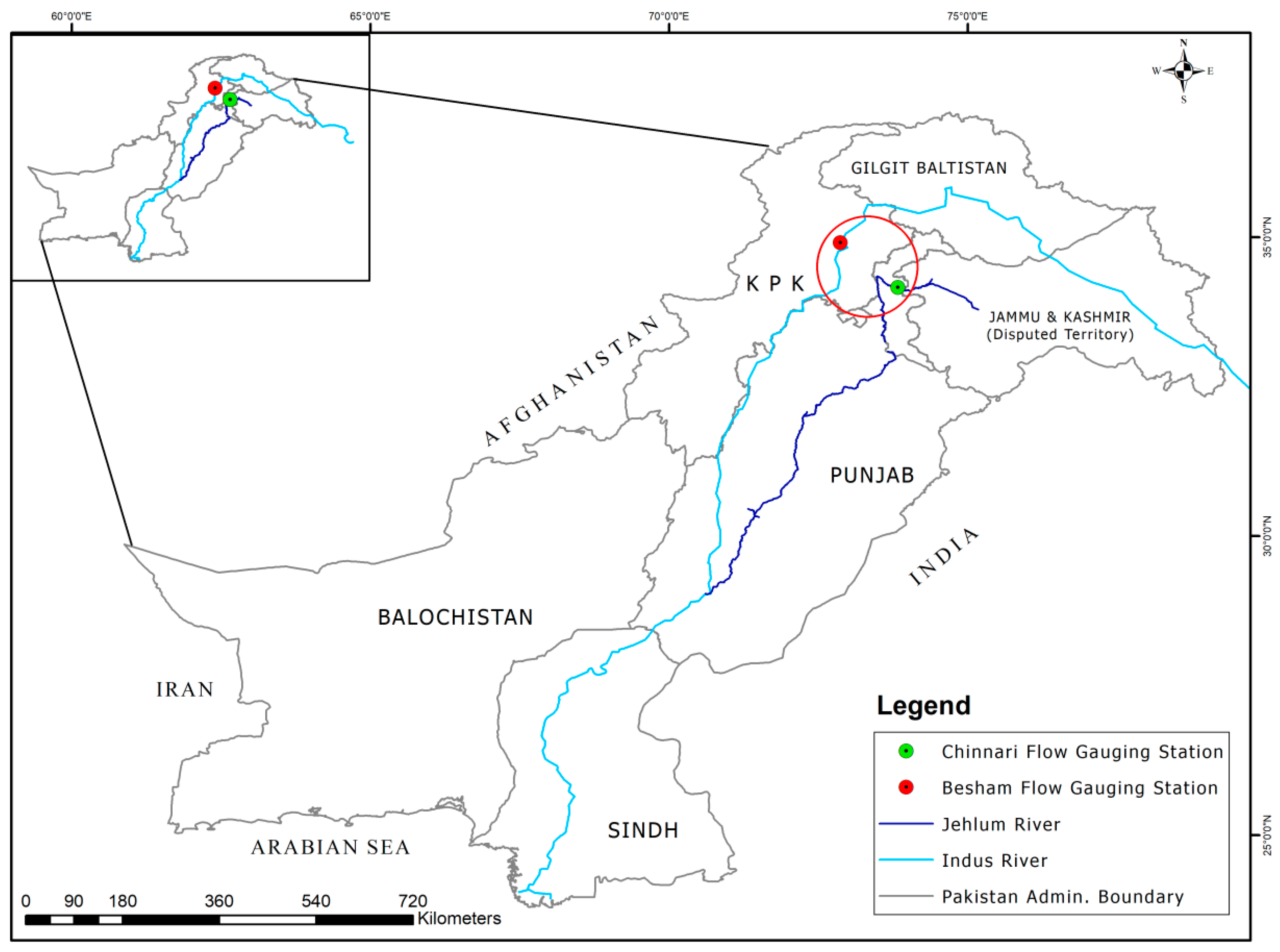
The study basin consists of two major rivers, Indus and Jhelum, in the Indus basin system of Pakistan. The Tarbela reservoir is the largest reservoir in Pakistan and it is fundamental to serving numerous purposes in the Indus basin. Besides hydropower generation, this dam allows for flood control facility and water reservation. It is located on the trans-boundary Indus river, which is one of the longest rivers in the world with a total length of 3200 km and a basin area of more than 1,165,000 km² stretched over four countries. It runs through the ranges and foothills of the Himalayas, the Hindu Kush, and the Karakoram, and stretches to the semiarid plains of Pakistan. The Mangla reservoir is another multi-purpose reservoir located on the Jhelum river in Pakistan. The Jhelum river emanates from Western Jammu and Kashmir and enters Pakistan, traversing a total length of 725 km. In this study, we obtained daily streamflow data of Indus and Jhelum rivers from the Water and Power Development Authority (WAPDA), Pakistan, covering a period of 1969–1997 for the Indus river and 1980–2013 for the Jhelum river. We probed the hydrological data by carrying out statistical tests which indicated that data was stationary and homogeneous for further analysis. The annual maximum flood discharge (Q), 3-day, 7-day and 15-day flood volumes (W_3d, W_7d, W_15d) were sampled. The sample statistics of mean, L-Cv and L-Cs were estimated and listed in

Table 1. Sample data statistics values of variables at Indus and Jhelum rivers.

River	Variable	Data Length (Years)	Sample Statistics Values
			Mean	L-Cv	L-Cs
Indus	Q (m3/s)	29	10,474.62	0.1384	0.6383
	W3d (108 m3)	29	2.651	0.1371	0.6817
	W7d (108 m3)	29	5.867	0.135	0.536
	W15d (108 m3)	29	11.67	0.147	0.369
Jhelum	Q (m3/s)	34	970.69	0.378	0.670
	W3d (108 m3)	34	0.229	0.349	0.345
	W7d (108 m3)	34	0.493	0.335	0.320
	W15d (108 m3)	34	0.976	0.334	0.382

. The values of l-skewness (L-Cs) as shown in Table 1 imply that the data is right-tailed while the coefficient of variance (L-Cv) suggests low variance of the data. The location of the Indus and Jhelum rivers is demonstrated in Figure 1. The map indicates the flow gauging stations besides the provincial and administrative boundaries of Pakistan. The gauging station on the Indus river is located at Besham, while the gauging station on the Jhelum river is located at Chinari as shown in Figure 1.

3. Methods

This study focuses on the derivation of DFH using multivariate analysis. The hydrological variables are associated through copula function to achieve a reliable estimation of flood variables. Later, the joint behaviors of flood variables are plotted. We adopted the following procedure: (i) Selection of the marginal distribution, (ii) comparing copulas from different families, (iii) deriving joint design floods based on the best-fit copula, and (iv) developing DFH by using the two combination methods based on the copula function. The schematic procedure is charted in Figure 2 for illustration.

3.1. Selection of Marginal Distribution

We selected the Indus and Jhelum rivers in Pakistan for carrying out the goodness-of-fit test to develop a convincing opinion about the most reliable PD. The details of the recorded data are provided in Table 1. First, we chose various commonly-used PDs, namely Pearson type III (P3), Weibull (WEI), generalized extreme value (GEV), generalized logistic (GLO), generalized Pareto (GPA), and generalized normal (GNO) for assessing their conformity to the empirical record of river basins in Pakistan. Since linear moment (LM) offers modest bias of an estimator, therefore we engaged linear moment (LM) approach for the computation of parameters. Let the conceptual random sample X₁, X₂, …, X_r of size r from a continuous function be represented by the function $Q_X\left(u\right)={F^{-1}}_X\left(u\right)$, then let the order statistics be represented by X_1r ≤ X_2r ≤ … ≤ X_rr. Hosking (1990) defined the r_th l-moment as follows [33,34]:

$${\lambda }_r=r^{-1}{{\displaystyle \sum }}_{k=0}^{r-1}{\left(-1\right)}^k(\begin{array}{c}r-1\\ k\end{array})E\left(X_{r-kr}\right),$$

(1)

where the order of moment is denoted by r (r = 1, 2, …,), and

$$E\left(X_{tr}\right)=\frac{r!}{\left(t-1\right)!\left(r-t\right)!}{{\displaystyle \int }}_0^{1}Q\left(u\right)u^{t-1}{\left(1-u\right)}^{r-t}du,$$

(2)

where Q(u) is the quantile function and t denote integers (t = 0, 1, 2, …).

$${\tau }_2=\frac{{\lambda }_2}{{\lambda }_1},{\tau }_3=\frac{{\lambda }_3}{{\lambda }_2},{\tau }_4=\frac{{\lambda }_4}{{\lambda }_2}.$$

(3)

The l-moment ratios, l-coefficient of variation (τ₂), l-skewness (τ₃), and l-kurtosis (τ₄) have been defined in Equation (3).

To evaluate the performance of PDs, we used the Akaike information criteria (AIC) and root mean square error (RMSE) as performance indicators to establish a convincing opinion about the goodness of PDs. AIC is an information-based criterion which encourages the selection of PDs under definite conditions [35,36]. On the other hand, RMSE is specifically referred to as measure the fit of PDs to the available record. Therefore, we coupled these criterions to examine the descriptive strength of PD_S and hence choose the most reliable marginal distribution. RMSE and AIC are defined by the following equations [37,38]

$$\mathrm{RMSE}=\sqrt{\frac{{{\displaystyle \sum }}_{i=0}^n{\left(P_{the}\left(i\right)-P_{emp}\left(i\right)\right)}^2}{n}},$$

(4)

$$\mathrm{AIC}=\left[ln\left[\frac{1}{n}{\displaystyle \sum }_{i=0}^n{\left(P_{the\left(i\right)}-P_{emp\left(i\right)}\right)}^2\right]\right]+2K,$$

(5)

where n is the size of the sample, K is the number of parameters of the distribution, P_the is the theoretical probability of the candidate distribution, and P_emp is empirical probability measured by the Gringorten plotting position formula [39],

$$P_{emp\left(i\right)=\frac{i - 0.44}{n + 0.12}}.$$

(6)

To measure comparative performances of PDs, we used Equations (4) and (5) to compute the values of AIC and RMSE corresponding to each PD. The candidate distributions receiving lower AIC and RMSE values are referred to as the best-fit PD.

3.2. Traditional Methods of Deriving DFH

The DFH derivation methods have been employed in numerous recent researches. These methods have been classified into four distinct classes by Yue et al. (2002) [40], namely: (i) The tradition unit hydrograph (TUH) method, (ii) the synthetic unit hydrograph (SUH) method, (iii) the typical flood hydrograph (TFH) method, and (iv) the statistical method (SM). These are discussed below.

i. The TUH method is focused on the assumptions of linear response of runoff to net rainfall and spatial homogeneity. Usually, the rainfall data is utilized in the TUH method to derive a DFH [41]. De Michele (2005) presented a traditional TUH method for constructing DFH by estimating flood peak and volume [42]. This method expects the area mean rainfall to represent the precipitation data for constructing DFH at a given basin which is a very rare event.

ii. The SUH method usually takes into account the triangular shape of the hydrograph in which the shape variables are estimated on the basis of watershed characteristics and practical experience [43]. In practice, the triangular shape of the hydrograph is very rarely achieved.

iii. The TFH method is frequently used by engineers for deriving DFH [40]. TFH with the largest flood peaks or volumes are mostly chosen to derive DFH. The construction of DFH takes place by multiplying each discharge ordinate by an amplifier. The amplifier is either the ratio of the design peak with a given return period to the TFH peak or the ratio of the design volume with a given return period to the TFH volume.

iv. The SM method usually engages PDFs such as gamma and β PDFs to illustrate the shape of a hydrograph [44]. The parameters of PDFs are estimated either from empirical flood hydrographs by the least-square method or by practical observation of goodness-of-fit of PDFs to the observed flood hydrograph. This method is constrained for lacking a systematic approach required to illustrate the statistics of flood hydrograph.

3.3. Peak and Volume Amplitude Method

The peak and volume amplitude method is currently practiced in Pakistan for estimating DFH. This method allows the flood peak and volume to be amplified with the same frequency. Let the flood characteristics of a hydrograph be represented by flood peak Q, 1-day maximum flood volume (W₁), 3-day maximum flood volume (W₃), 7-day maximum flood volume (W₇), and 15-day maximum flood volume (W₁₅). The design quantiles are estimated for design return period T by an FFA model, estimated usually with the goodness-of-fit test or by empirical knowledge. The design flood quantiles estimated by a univariate model for a design return period are denoted by Q_D, W_1D, W_3D, W_7D, and W_15D respectively and the corresponding variables of TFH are denoted by Q_T, W_1T, W_3T, W_7T, and W_15T. Later, the sections of TFH are amplified to derive DFH that are calculated as follows.

Amplifier K_P for flood peak:

$$K_P=\frac{Q_D}{Q_T}.$$

(7)

Amplifier K₁ for the 1-day maximum flood volume (excluding flood peak):

$$K_1=\frac{W_{1D}}{W_{1T}}.$$

(8)

Amplifier K_3–1 for the 3-day maximum flood volume excluding the 1-day maximum flood volume:

$$K_{3-1}=\frac{W_{3D}-W_{1D}}{W_{3T}-W_{1T}}.$$

(9)

Amplifier K_7–3 for the 7-day maximum flood volume excluding the 3-day maximum flood volume:

$$K_{7-3}=\frac{W_{7D}-W_{3D}}{W_{7T}-W_{3T}}.$$

(10)

Amplifier K_15–7 for the 15-day maximum flood volume excluding the 7-day maximum flood volume:

$$K_{15-7}=\frac{W_{15D}-W_{7D}}{W_{15T}-W_{7T}}.$$

(11)

Hand smooth treatment is imperative to adjust the dividing portion between two contiguous sections of DFH in practice.

3.4. Deriving Joint Design Floods Based on Copulas

The conventional univariate method considers the random variables required to construct a DFH as independent, and does not take into account the inherent relationship between the random variables. Copula function identifies the interdependence structure among the flood variable and associates them to derive a joint probability distribution of the flood variables [45,46,47]. Let the cumulative distribution function (CDF) of X_i be represented by F_xi (x_i) (i = 1, 2, …, n). To obtain a multivariate probability distribution expressed as H_X1, _X2, _Xn(x₁, x₂, …, x_n) or simply H, the Sklar’s theorem is applied to determine the marginal and joint function as shown below:

𝐶{𝐹_X1 (𝑥₁), 𝐹_X2 (𝑥₂), …, 𝐹_X𝑛 (𝑥_𝑛)} = 𝐻_X1,_X2, …,_Xn (𝑥₁, 𝑥₂, …, 𝑥_𝑛),

(12)

where C denotes the Copula function that determines and typifies the associated dependence among flood variables. The application of the copula function to model hydrological events is based on its success in other fields like finances. To model multivariable events like droughts, storms and floods Archimedean and extreme value copulas are mostly used. Given the smooth construction of bivariate models of hydrological events, the Archimedean copula is largely employed. The Archimedean copula contains a broad class of copulas to model the joint PDF of hydrological events.

In this study, we have used Frank, Gumbel-Hougaard (G-H) and Clayton copulas belonging to the Archimedean family of copulas to design the joint PDF of flood events in Pakistan. The Archimedean bivariate copula functions, correlation between their parameters, and Kendall correlation coefficient listed in

Table 2. Bivariate copula functions and the association between their parameters and Kendall correlation coefficient.

Copula Function	${\mathbf{C}}_{\mathsf{\theta }}\left(\mathbf{u}, \mathbf{v}\right)$	$\mathsf{\theta }\in$	$\mathsf{\tau }$
Gumbel-Hougaard	$\exp \left\{-{\left[{\left(-\mathrm{lnu}\right)}^{\mathsf{\theta }}+{\left(-\ln \mathrm{v}\right)}^{\mathsf{\theta }}\right]}^{\frac{1}{\mathsf{\theta }}}\right\}$	$\left(1,\infty \right)$	$1-{\mathsf{\theta }}^{-1}$
Clayton	${({\mathrm{u}}^{-\mathsf{\theta }}+{\mathrm{v}}^{-\mathsf{\theta }}-1)}^{\frac{-1}{\mathsf{\theta }}}$	$\left(0,\infty \right)$	$\frac{\mathsf{\theta }}{\mathsf{\theta }+2}$
Frank	$-\frac{1}{\mathsf{\theta }}\ln \left[1+\frac{\left({\mathrm{e}}^{-\mathsf{\theta }\mathrm{u}}-1\right)\left({\mathrm{e}}^{-\mathsf{\theta }\mathrm{v}}-1\right)}{{\mathrm{e}}^{-\mathsf{\theta }}-1}\right]$	$\mathrm{R}\setminus \left\{0\right\}$	$\mathsf{\tau }=1+\frac{4}{\mathsf{\theta }}\left[\frac{1}{\mathsf{\theta }}\underset{0}{\overset{\mathsf{\theta }}{{\displaystyle \int }}}\frac{\mathrm{t}}{\exp \left(\mathrm{t}\right)-1}\mathrm{dt}-1\right]$

are used to model the flood event.

The pertinent combination of hydrological variables for a given return period is significant since the different combinations of flood quantiles would produce different DFHs [13,48,49]. Therefore, the selection of appropriate composition methods for deriving flood quantiles is crucial in practice. Moreover, the DFH is rescaled by modifying the discharge ordinates with the same frequency in traditional univariate flood frequency analysis [17]. Under the given discharge, the probability of occurrence differs under particular combinations of flood quantiles. Therefore, we have used copula-based MLC and EFC methods to derive joint flood quantiles. These combination methods are presented as follows:

3.4.1. EFC Method

To represent the combination of hydrological values for a given bivariate return period T, the EFC method is used to derive the bivariate flood quantiles. With the assumption of flood peak and flood volume having the same probability of occurrence i.e., u = v (or F_Q(q) = F_W(w)), the design frequency of bivariate EFC is achieved by jointly solving u = v and

$${\mathrm{C}}_{\mathsf{\theta }}\left(\mathrm{u},\mathrm{v}\right)=\exp \left\{-{\left[{\left(-\mathrm{lnu}\right)}^{\mathsf{\theta }}+{\left(-\ln \mathrm{v}\right)}^{\mathsf{\theta }}\right]}^{\frac{1}{\mathsf{\theta }}}\right\}=1-\frac{1}{\mathrm{T}}.$$

(13)

Based on the equal probability of occurrence of bivariate flood quantiles, these quantiles are expressed as follows [50]:

$$\mathrm{u}=\mathrm{v}={\left(1-\frac{1}{\mathrm{T}}\right)}^{\mathsf{\zeta }},$$

(14)

where ζ= $2^{\frac{-1}{\mathsf{\theta }}}$, and θ is the dependence parameter of the G–H copula.

Therefore, the design values of hydrological quantiles are obtained by the inverse function of marginal distributions:

$$q=F_Q^{\left(-1\right)}\left(\mathrm{u}\right),w=F_W^{\left(-1\right)}\left(\mathrm{v}\right),$$

(15)

3.4.2. MLC Method

In this paper, we used the MLC method proposed by Salvadori and Michele [49] to study the inherent relationship between hydrological variables. For MLC, the joint quantiles ($q^{*}, w^{*}$) can be calculated by choosing the largest joint probability density for all possible events [49,51]:

$$\left(q^{*}, w^{*}\right)=\mathrm{argmax}f \left(q, w\right)=\mathrm{c}\left[F_Q\left(q\right), F_W\left(w\right)\right]f_Q\left(q\right)f_W\left(w\right)C\left(u, v\right)=t,$$

(16)

where hydrological variables flood peak and volume are represented by a joint PDF f(q, w),$\mathrm{c}\left(\mathrm{u},\mathrm{v}\right)=\frac{\mathrm{dC}\left(\mathrm{u},\mathrm{v}\right)}{\mathrm{dudv}}$ is the density function of copula, $f_Q\left(q\right)$ is the PDF of $F_Q\left(q\right),$ and $f_W\left(w\right)$ is the PDF of $F_W\left(w\right)$. We used the Lagrange multiplier method to get the joint design quantile along the level curve. The Lagrange function under one JRP is represented as below

$$\phi \left(q, w\right)=\left(F_Q\left(q\right), F_W\left(w\right)\right)f_Q\left(q\right)f_W\left(w\right)+\mathsf{\lambda }\left[\mathrm{C}\left[F_Q\left(q\right), F_W\left(w\right)\right]-\left(1-\frac{1}{T_{or}}\right)\right].$$

(17)

The first order derivative equals zero when reaches the maximum value and the following equations should be satisfied

$${\phi }_q=\left[c_q{f}^2\left(q\right)+\mathrm{c}\left(\mathrm{u},\mathrm{v}\right){\mathrm{f}}_{\mathrm{Q}}^{\prime }\left(q\right)\right]f_W\left(w\right)+\lambda \frac{\partial C\left[F_Q\left(q\right), F_W\left(w\right)\right]}{\partial q}=0,$$

(18)

$${\phi }_W=f_W\left(w\right)\left(c_w{f}_W^2\left(w\right)+c\left(u, v\right)f_W^{,}\left(w\right)\right)+\lambda \frac{\partial C\left[F_Q\left(q\right), F_W\left(w\right)\right]}{\partial w}=0.$$

(19)

where λ is Lagrange multiplier, $c_q=\frac{\partial \mathrm{c}\left(\mathrm{u},\mathrm{v}\right)}{\partial \mathrm{u},c_w}=\frac{\partial \mathrm{c}\left(\mathrm{u},\mathrm{v}\right)}{\partial \mathrm{v}}$.

The above non-linear equations could be solved by the harmonic mean Newton’s method and several other mathematical approaches [52].

3.5. Joint Return Period

In the domain of conventional univariate analysis, desirable hydrological quantiles are represented by return periods. However, hydrologists still investigate the transformation of joint exceedance probability to a bivariate joint return period (JRP) of hydrological quantiles. Copula function has dealt with different return periods for bivariate analysis of hydrological quantiles. Salvadori and De Michele [24] provided eight possible joint events using “OR” and “AND” operators that are frequently applied in the multivariate domain.

(1)

“OR” case, either Q > q or W > w, i.e.,

$${\mathrm{E}}_{\mathrm{or}}=\left\{Q>q\hspace{1em}or\hspace{1em}W>w\right\}.$$

(20)

(2)

“AND” case, both Q > q or W > w, i.e.,

$${\mathrm{E}}_{\mathrm{and}}=\left\{Q>q\hspace{1em}and\hspace{1em}W>w\right\}.$$

(21)

For E_or scenario, one of the flood variable (Q or W) may exceed the arbitrary values but for E_and scenario, it is required that both the flood variables (Q and W) exceed the recommended level. Therefore, the two different bivariate return periods are defined as follows [42]:

$$T_{or}=\frac{\mu }{P\left[Q>q\hspace{1em}or\hspace{1em}W>w\right]}=\frac{\mu }{1-F\left(q, w\right)},$$

(22)

$$T_{and}=\frac{\mu }{P\left[Q>q\hspace{1em}and\hspace{1em}W>w\right]}=\frac{\mu }{1-F\left(q, w\right)},$$

(23)

where μ is the mean inter-arrival between two executive events (in the case of annual maxima μ =1 year), and F (q, w) =$P\left(Q\le q, W\le w\right)$.

Various definitions of multivariate return periods have been provided in the literature depending upon the different functions, such as bivariate conditional distribution, regression analysis, survival Kendal distribution function, conditional distributions, and structure performance function. The multivariate return periods like the structure-based return period have been involved for design and/or risk assessment of critical hydraulic structures in a bivariate domain [12]. Another multivariate return period known as the Kendall return period was also introduced by Salvadori and Michele (2004) [24]. This return period focused on the identification of a univariate critical threshold in a multivariate context. This return period is rarely used in studies, whereas the hydrologists have greatly utilized the “OR” return period to investigate the multivariate quantiles [13,16,53]. In this study, we practiced the “OR” return period for bivariate quantile estimation.

3.6. Procedure for DFH Generation

We employed the MLC and EFC methods based on copula function to derive the design flood quantiles of hydrological pairs. A flood of reasonable enormity conforming to the design standards of the dam is fundamental to protect the structure; therefore, derivation of DFH is essential to protect the reservoir from the risk of floods. To this effect, we selected the annual maximum flood hydrograph of the Indus and Jhelum rivers as the typical flood hydrograph (TFH) from the annual streamflow data of several years. The bivariate hydrological quantiles ($q_T$,$w_T$) were generated by applying the combination methods. Later, we transformed the computed design flood quantiles to corresponding DFH by amplifying the TFH. The stepwise procedure to ascribe shape to observed hydrograph by amplification is illustrated as follows [12]:

(1)

The ratio $r_T=\frac{q_T}{w_T}$ between the hydrological pairs of flood peak and volume is determined.

(2)

The normalized ratio R_T varying within (0, 1) is estimated by:

$$R_T=\frac{r_T-mi{n}_{rT}}{ma{x}_{rT}-mi{n}_{rT}},$$

(24)

whereas maximum and minimum values are represented by $ma{x}_{rT}$ and $mi{n}_{rT}$ respectively.

(3)

The normalized ratio between M hydrological pairs of the observed hydrograph is also determined using steps 1 and 2 and is represented as $R_k$, k = 1, …, M.

(4)

The square sum of deviations $S{S}_{TK}$ between $R_T$ and $R_k$ for M pairs are calculated as follows for each simulated hydrological pair ($q_T$, $w_T$) covered by single JRP ${\mathrm{T}}_{\mathrm{or}}$.

(5)

The observed TFH offering narrowest ratio (min) is chosen.

(6)

The hydrological pair ($q_T$, $w_T$) is transformed into corresponding DFH by amplifying the selected observed TFH values.

$$\mathrm{DFH}=\left(\mathrm{TFH} \left(t\right)-Q_D\right)\times (\frac{w_T}{DT - q_T})/(\frac{W_D}{DT - q_T})+q_T,$$

(25)

where DFH is the desired design flood hydrograph resulting from amplification of the observed hydrograph and TFH is observed discharge, against time t respectively. $W_D$ is flood volume of observed values against a 15-day flood duration $DT$; $Q_D$ is the peak flow of observed hydrograph.

The amplification in the above-mentioned procedure procures hydrological quantiles identical to the designated values without making any modification to the flood duration. Therefore, this method of ascribing shape to DFH is more useful [31].

4. Application and Discussion

The schematic procedure to develop DFH is applied to the two major rivers in Pakistan. To derive DFH, we employed the copula function to couple the hydrological quantiles and presented results in the following section. The results have been graphically supported to determine the fitting of the methods.

4.1. Selection of Marginal Distribution

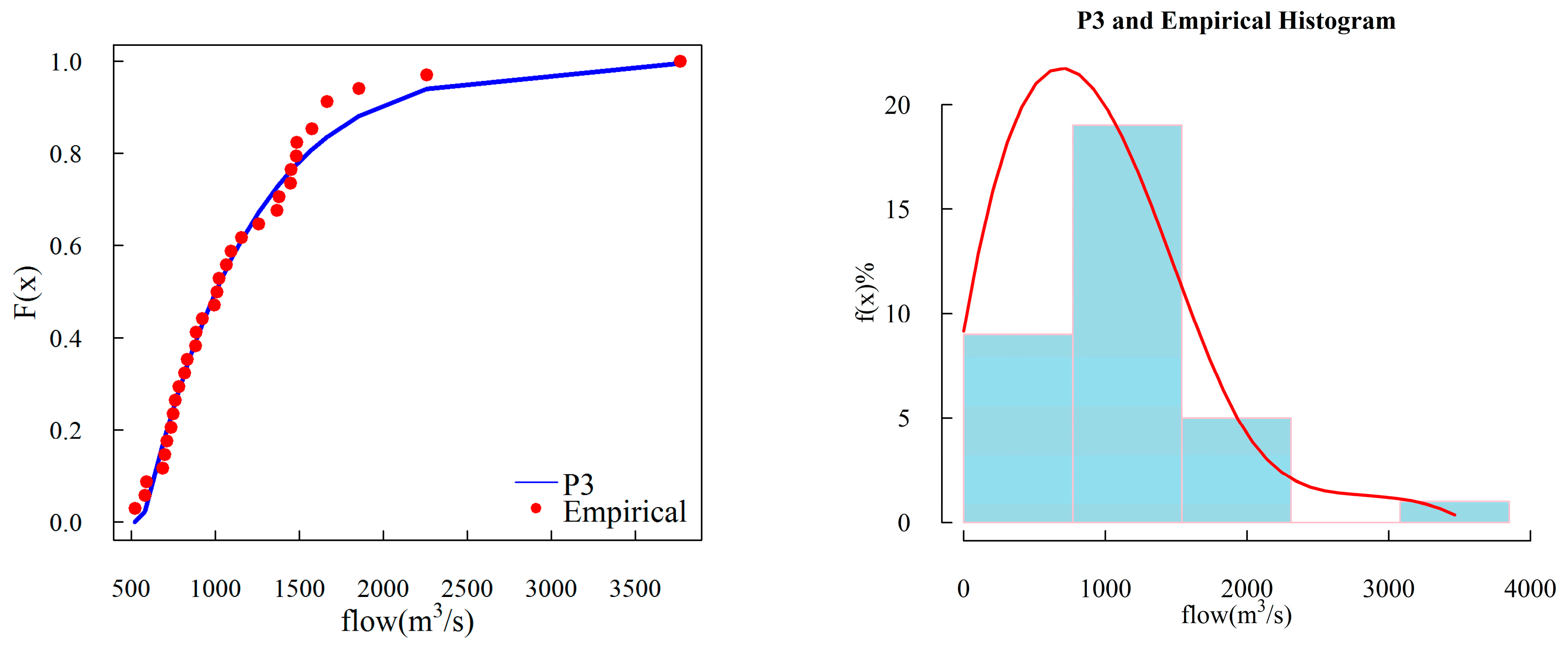
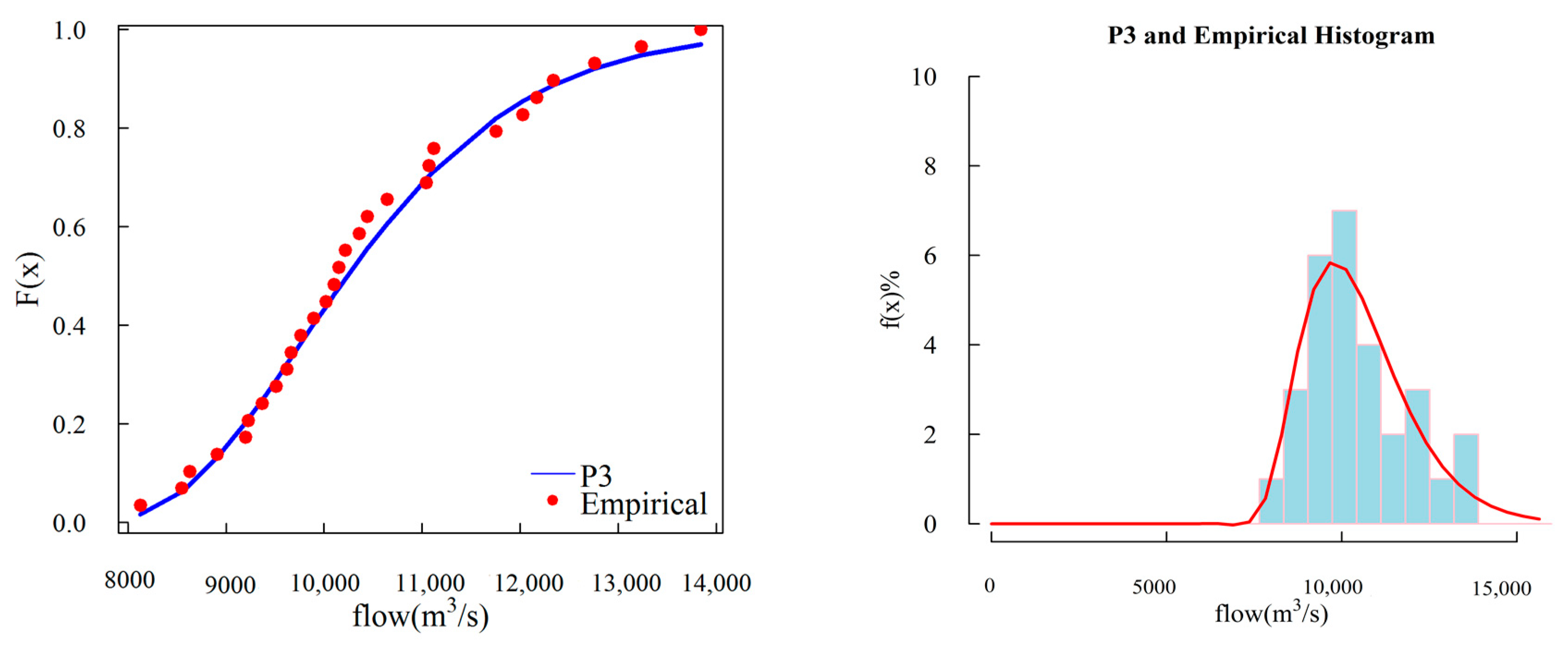
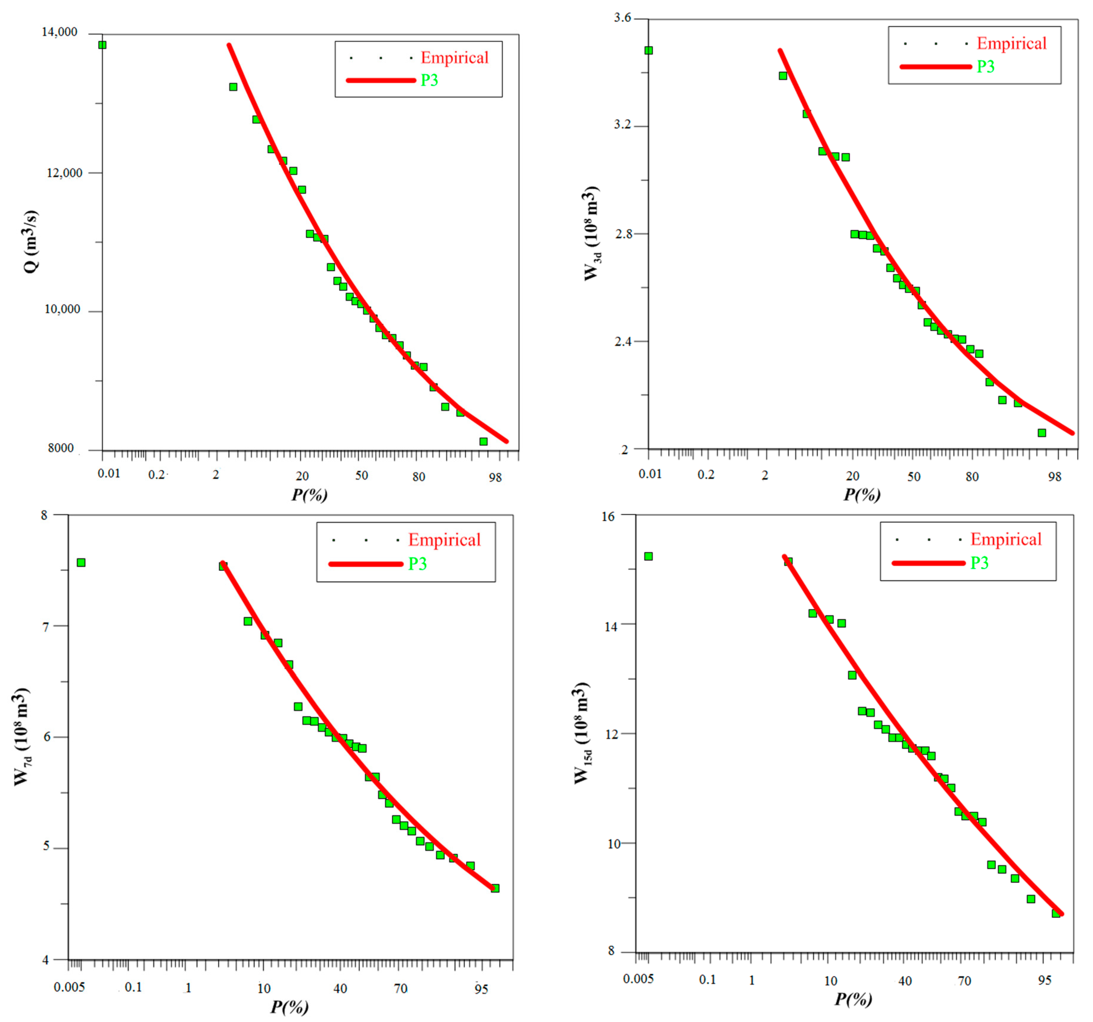
In order to assess the performance of PDs, we used the goodness-of-fit criterion, involving RMSE and AIC, to probe various familiar PDs. We used the annual maximum flow record of the Indus and Jhelum rivers to evaluate the performance of PDs by measuring the performance indicators of candidate PDs. The results, as indicated in

Table 3. Akaike information criteria (AIC) and root mean square error (RMSE) values of statistical distributions.

Location	Criteria	Probability Distributions
		GPA	GNO	GLO	WEI	P3	GEV
Indus River	AIC	−184.90	−199.85	−191.44	−197.11	−199.90	−200.18
	RMSE	0.0372	0.02874	0.0332	0.03013	0.0287	0.02858
Jhelum River	AIC	−223.05	−229.96	−216.66	−224.79	−225.68	−224.70
	RMSE	0.0344	0.0311	0.0378	0.0335	0.0331	0.0336

, demonstrates the goodness of the P3 distribution with the lowest RMSE and AIC values for the Jhelum river, and establishes a better fit to the empirical record of the Indus river as well. The GPA exhibited slightly higher values of AIC and RMSE for the Jhelum river relative to P3 distribution and slightly lower values at Indus river. Therefore, in order to select one model, we chose P3/LM to estimate the design values, and in order to support our findings we plotted P3 distribution and empirical frequency of selected rivers in Figure 3 and Figure 4. The dots represent the empirical frequencies while the lines represent the theoretical frequencies of the P3 distribution. From Figure 3 and Figure 4, it is determined that the theoretical CDF of P3/LM fit the empirical CDF for both locations and the PDF of P3 distribution also fit the empirical histogram of the flow record for both rovers. After acquiring ample evidence, we employed P3 distribution to develop flood frequency curves of peak flow, 3-day flood volume, 7-day flood volume and 15-day flood volume using the Weibull plotting formula to evaluate the linearity for the empirical record in Figure 5 which shows a good correspondence between empirical and theoretical frequencies. These graphical representations indicate the fitting of the P3 distribution to observed data.

4.2. Comparison of Copulas

The joint behavior of different variables may be defined by copulas from different families. Nelsen (2006) have proposed such copula families to define hydrological analysis [46]. The Archimedean copula family is of major interest to hydrologists on account of its smooth construction and application irrespective of correlation between the hydrological variables [46,54]. We applied Gumbel-Hougaard (G–H), Clayton and Frank copulas to construct bivariate association of flood peak and volume. Additionally, to estimate parameters of copulas, different methods are available. However, we used the inversion of Kendall’s tau $(\tau )$ to determine the parameters of bivariate copulas.

The association between parameters and Kendall’s correlation coefficient is manifested in Table 2. The Kendall’s τ yielded 0.96, 0.81 and 0.61 for hydrological pairs of Q_max-W_3d, Q_max-W_7d, and Q_max-W_15d on the Indus river and 0.93, 0.84 and 0.78 for the same pairs on the Jhelum river. Next, we applied statistical tests to compare the copulas from Archimedean family. We calculated p-values using the parametric bootstrap based procedure with 10,000 runs to confirm the suitability of the bivariate copula model and carried out the Kolmogorov-Smirnov test (K-S) for determining the fitting copula as manifested in

Table 4. Parameters of copulas and values of statistical test for determining suitable copula.

River	Variable	G–H			Clayton			Frank
		θ	Dn	Pv	θ	Dn	Pv	θ	Dn	Pv
Indus	Qmax-W3d	22.56	0.031	0.012	43.11	0.037	0.024	88.55	0.039	0.022
	Qmax-W7d	5.21	0.032	0.023	8.41	0.039	0.029	19.02	0.035	0.031
	Qmax-W15d	2.57	0.028	0.031	3.14	0.030	0.035	8.23	0.037	0.029
Jhelum	Qmax-W3d	14.38	0.033	0.024	26.77	0.039	0.029	55.84	0.037	0.033
	Qmax-W7d	6.45	0.029	0.039	10.90	0.040	0.033	24.03	0.035	0.041
	Qmax-W15d	4.49	0.031	0.033	6.98	0.033	0.035	16.12	0.038	0.037

that illustrates the estimated parameters of candidate copulas (θ), Kolmogorov-Smirnov test (D_n) and p-values (Pv). On the basis of the statistical test, we found that the G–H copula is best suited to define the multivariate phenomenon and model the joint probability density function. Therefore, we investigated the hydrological pairs by applying G–H copula. Additionally, the use of MLC and EFC methods based on G–H copula for deriving the joint density function of hydrological pair is in consonance with the findings.

4.3. Derivation of DFH

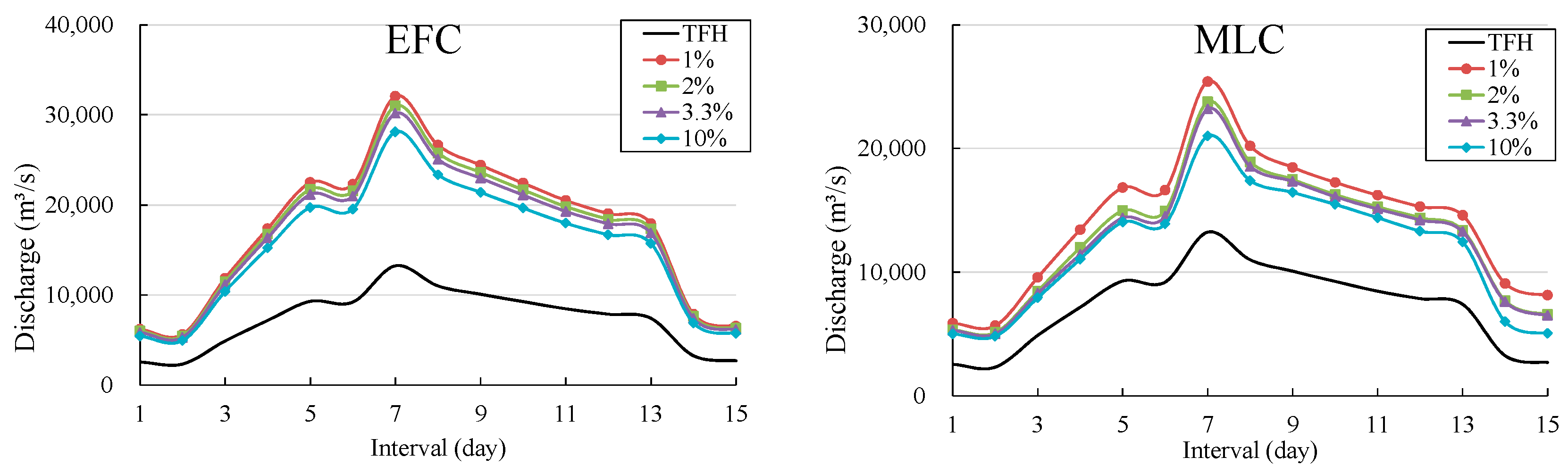
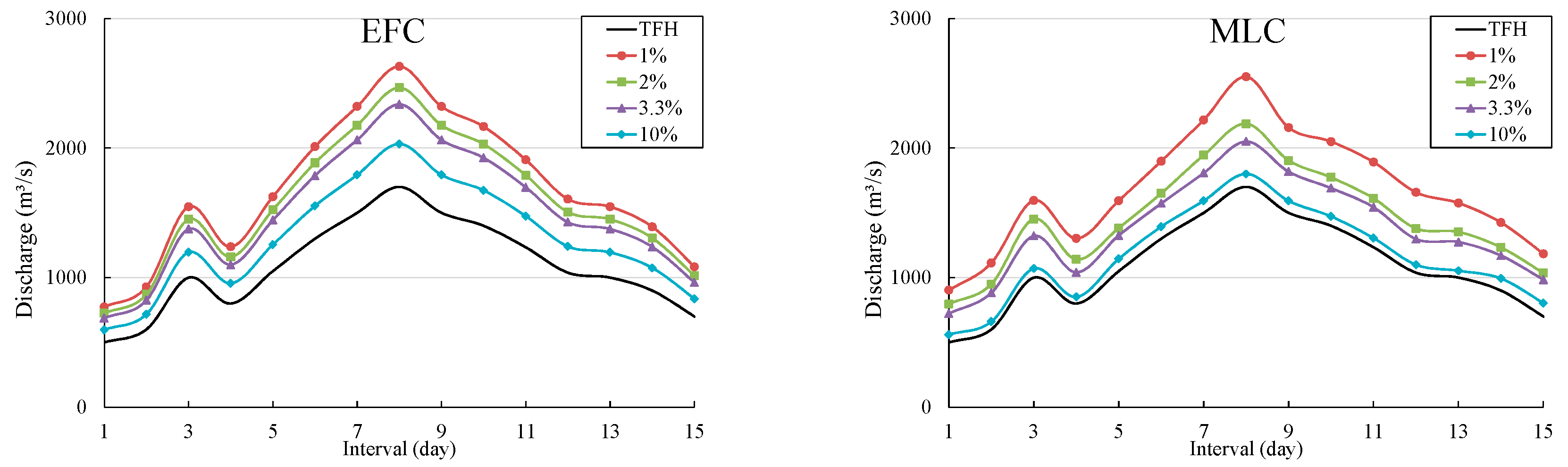
The derivation of DFH took place by employing the two combination methods for return periods of 100, 50, 30 and 10 years. The two methods were used to compute the design flood peaks and volumes for different return periods. Firstly, we selected TFH for both rivers based on peak flow, volume, and the enormity of flow. We selected the observed flood hydrographs of 1994 for the Indus river and 1992 for the Jhelum river that secured high peaks, and higher flood volumes with posterior-peak shape that may threaten the downstream basins and endanger safety of reservoirs. We also engaged the univariate model (P3/LM) to determine the design values of flood characteristics (Q, W_3d, W_7d, W_15d) for given return periods of 10, 30, 50 and 100 years and listed them in

Table 5. Comparison of flood quantiles estimated by different methods.

River		Indus				Jhelum
Return Period		100	50	30	10	100	50	30	10
Q (m3/s)	P3/LM	14,975	14,267	13,729	12,491	2117	1935	1798	1481
	MLC	15,229	14,842	14,084	12,606	2080	1918	1796	1512
	EFC	15,942	15,143	14,711	12,993	2157	1977	1839	1527
W3D (108 m3)	P3/LM	3.68	3.52	3.34	3.14	0.46	0.42	0.40	0.34
	MLC	3.75	3.62	3.46	3.18	0.47	0.43	0.41	0.34
	EFC	3.71	3.57	3.42	3.16	0.47	0.43	0.40	0.34
W7D (108 m3)	P3/LM	8.02	7.78	7.55	6.75	0.96	0.89	0.84	0.72
	MLC	8.25	7.98	7.68	7.02	0.99	0.92	0.86	0.74
	EFC	8.21	7.90	7.59	6.95	0.97	0.90	0.85	0.73
W15D (108 m3)	P3/LM	16.3	15.6	15.1	14.0	1.87	1.75	1.65	1.42
	MLC	16.6	15.9	15.4	14.3	1.95	1.82	1.71	1.46
	EFC	16.3	15.7	15.3	14.2	1.90	1.78	1.68	1.45

. Later, we employed MLC and EFC methods to derive bivariate design flood quantiles of Q_max-W_3d, Q_max-W_7d,and Q_max-W_15d under one JRPor for required return periods of 100, 50, 30 and 10 years. Next, we amplified the observed flood hydrograph with the amplification procedure discussed in Section 3.6. Accordingly, we used Equation (25) to amplify the observed hydrograph. Next, the DFHs for 100, 50, 30, and 10 years are rescaled with the bivariate EFC and MLC methods. Subsequently, the DFHs using both combination methods are developed and demonstrated in Figure 6 for the Jhelum river and Figure 7 for the Indus river in Pakistan. Since the flood characteristics and flood control characteristics of the investigated catchment determine the flood duration [55], therefore we selected Q_max-W_15d DFH for both combination methods based on the flood characteristics of the investigated catchment and flood regulation characteristics of reservoirs in Pakistan. It is determined from the DFHs that the two combination methods demonstrated few differences by developing contrasting hydrographs. From Figure 6, it can be inferred that the DFH obtained with EFC method has higher peaks than the MLC method. Design peak of the DFH of EFC method is larger than the design peak of MLC method to the extent of 24%. Furthermore, Figure 7 demonstrated DFHs obtained with the two combination methods at Jhelum river and it is evident that the peak of the DFH achieved by EFC method is larger than the MLC method. The peak of EFC exceeds the design peak of MLC method by 5%. In addition to that, the EFC method observed a considerable difference with the TFH as evident from Figure 6 and Figure 7. TFH is an observed hydrograph whose shape may pose a threat to the downstream section [31,56] and the EFC considers the equivalent frequency of the occurrence probability of hydrological quantiles, therefore, the DFH obtained by the EFC method is considerably larger. In this context, the EFC method advanced a relatively greater difference with TFH than MLC method on both rivers as indicated in Figure 6 and Figure 7. Moreover, the difference between the DFHs for Jhelum river is minimal when compared to the DFH for the Indus river.

The quantiles of design flood peaks and flood volumes estimated by EFC method and MLC method for different JRPs and corresponding design values estimated by univariate model (P3/LM) against different return periods are also listed in Table 5. It is determined from Table 5 that design values of flood peaks and volumes estimated by the univariate model are smaller than the EFC method and the MLC method. However, there is a marginal difference between the flood peaks and volumes acquired by the EFC and MLC method. Furthermore, EFC acquired higher design flood peaks than the MLC method and the difference is translated to DFHs where the larger design value of peaks resulted in larger DFH than the MLC method. In addition to that, it is also inferred that design flood volumes obtained by the MLC method are higher than EFC method. Summing up, the resulting design values of the univariate method are relatively smaller than those bivariate approaches. Therefore, from the above discussion, it can be argued that the quantiles estimated by the univariate model are an underestimation of flood risk and EFC method securing higher design flood peaks than the two methods can be trusted to provide reliable design values of the proposed dam. Although EFC method may result in greater volume of the dam, it is still a safer option to design a flood control system in order to avoid the potential catastrophic effects of the flood events. In addition to that, the EFC method rationalizes the multivariate nature of flood event by mutually correlating hydrological variables. Hence, it is reliable to use this method in engineering practices for the design of critical hydraulic structures like dams in Pakistan because of its better risk assessment of catastrophic flood events.

4.4. Discussion

The formation of a suitable DFH is of paramount importance for the construction of dams. Our work is an attempt to update the shape of DFH in Pakistan as it deviates from the conventional methods. The conventional univariate analysis method presents ease in deriving DFH but it overlooks the risks involved by ignoring the correlation between hydrological variables. Hydrologic design is carried out to regulate water use and evaluate the impact of hydrological events on hydrologic structures such as dams. To secure the safe hydrologic design of structures, the extreme events are analyzed to estimate the risk associated with these catastrophic events. Since univariate frequency analysis focus on a single flood variable i.e., peak discharge, it fails to measure the true risk associated with the flood events. To take into account multiple variables of hydrological events for improved risk analysis, many authors have carried out studies focusing on multivariate methods for deriving design flood quantiles. Multivariate studies of any sort have hardly been carried out in Pakistan, where there is a huge potential for hydropower projects that necessitates multivariate analysis to manage the water resource. Naz et al. (2016) carried out a multivariate study recommending the Gumbel mixed model for representing joint behavior of flood peaks and volumes on the Indus river in Pakistan [57]. However, in the multivariate domain, the marginal distribution belongs to the same family of distribution, and it therefore becomes difficult mathematically to estimate the multiple variables. To avoid this arbitrariness, we employed the copula function to define the relationship between hydrological quantiles and procure full evaluation of the probability of occurrence of the flood event. Additionally, the hydrologic design is carried out by assessing the impact of hydrologic events in a more rational way. Since floods are a multivariate phenomenon by nature where the flood peaks and volumes are mutually correlated, therefore we paid significant attention to pair the hydrological variables for updating the shape of DFH in Pakistan. In this way, our study may contribute to water resource management in the country. Additionally, it will pave the way for rational engineering practices in the country and replace the conventional univariate method.

5. Conclusions

In this study, we characterized the DFH generation by applying two bivariate quantile combination methods based on copula function. Therefore, to carry out the bivariate quantile estimation for DFH derivation, we advanced our study by engaging copula function for deriving hydrological variables that maintain the advantage over other multivariate methods by considering the dependence structure between random variables under a single joint return period. Beginning with quantifying the degree-of-fit of marginal distribution, we used six common PDs to determine their goodness-of-fit to the empirical record. The selection criteria consisted of AIC and RMSE for evaluating the performance of PDs used in this study. P3 distribution performed better by securing lower values of AIC and RMSE and fitting the empirical frequency curves. The theoretical CDF of P3/LM also fits the empirical CDF for both locations demonstrating the robustness of the P3 distribution. Moreover, the PDF of P3 distribution fits the empirical histogram of the flow record for both rovers as demonstrated in Figure 3 and Figure 4. In addition, the frequency curves of the P3 distribution are also linear to empirical frequencies demonstrating a fit to the observed data as shown in Figure 5.

Next, we evaluated the performances of different copulas belonging to the Archimedean family based on KS test values of Dn and p values. The bivariate joint distributions of G–H, Clayton, and Frank copulas were applied. The G–H copula performed better than other copulas of Archimedean family to characterize the relationship between flood peak and volume. Finally, we advanced our study by deriving joint design flood quantiles based on G–H copula and the bivariate hydrological quantiles were estimated by using the EFC and MLC methods based on G–H copula using JRPor of 100, 50, 30 and 10 years. After acquiring the design flood variables, we transformed the design quantiles into the DFH using the procedure discussed in Section 3.6. By acquiring higher design values than the MLC method, the EFC method can obtain the highest reservoir water level. Therefore, it can secure a safer design of spillways.

The combination methods, used to couple hydrological quantiles, present a very useful way of estimating bivariate quantiles under a joint return period. The introduction of the copula function for the formation of DFH creates a better prediction of the probability of occurrence, which will provide a new approach and a new scheme for the design of dams in Pakistan. The study can further be extended to evaluate the impact of bivariate quantile estimation uncertainty on the highest water reservoir levels based on copula.

References

- Yin, J.; Gentine, P.; Zhou, S.; Sullivan, C.S.; Wang, R.; Zhang, Y.; Guo, S. Large increase in global storm runoff extremes driven by climate and anthropogenic changes. Nat. Commun. 2018, 9, 4389. [Google Scholar] [CrossRef] [PubMed]
- ICOLD (International Congress on Large Dams). Selection of Design Flood; Bulletin Report 82; ICOLD: Paris, France, 1992. [Google Scholar]
- ASCE. Hydrology Hand-Book, 2nd ed.; Manuals and Reports on Engineering Practices No. 28; ASCE: Reston, VA, USA, 1996. [Google Scholar]
- Yin, J.; Guo, S.; He, S.; Guo, J.; Hong, X.; Liu, Z. A copula-based analysis of projected climate changes to bivariate flood quantiles. J. Hydrol. 2018, 566, 23–42. [Google Scholar] [CrossRef]
- U.S. Water Resources Council (USWRC). Guidelines for Determining Flow Frequency, Bulletin 17B; U.S. Water Resources Council (USWRC): Washington, DC, USA, 1981.
- MWR (Ministry of Water Resources). Regulation for Calculating Design Flood of Water Resources and Hydropower Projects; Water Resources & Hydropower Press: Beijing, China, 2006. (In Chinese) [Google Scholar]
- Vittal, H.; Singh, J.; Kumar, P.; Karmakar, S. A framework for multivariate data-based at-site flood frequency analysis: Essentiality of the conjugal application of parametric and nonparametric approaches. J. Hydrol. 2015, 525, 658–675. [Google Scholar] [CrossRef]
- Smith, K. Environmental Hazards: Assessing Risk and Reducing Disaster; Routledge: Abingdon, UK, 2003. [Google Scholar]
- Chen, L.; Singh, V.P.; Shenglian, G.; Hao, Z.; Li, T. Flood coincidence risk analysis using multivariate copula functions. J. Hydrol. Eng. 2011, 17, 742–755. [Google Scholar] [CrossRef]
- Li, T.; Guo, S.; Chen, L.; Guo, J. Bivariate flood frequency analysis with historical information based on copula. J. Hydrol. Eng. 2012, 18, 1018–1030. [Google Scholar] [CrossRef]
- Liu, P.; Li, L.; Guo, S.; Xiong, L.; Zhang, W.; Zhang, J.; Xu, C.-Y. Optimal design of seasonal flood limited water levels and its application for the Three Gorges Reservoir. J. Hydrol. 2015, 527, 1045–1053. [Google Scholar] [CrossRef]
- Requena, A.I.; Mediero, L.; Garrote, L. A bivariate return period based on copulas for hydrologic dam design: Accounting for reservoir routing in risk estimation. Hydrol. Earth Syst. Sci. 2013, 17, 3023–3038. [Google Scholar] [CrossRef]
- Volpi, E.; Fiori, A. Design event selection in bivariate hydrological frequency analysis. Hydrol. Sci. J. 2012, 57, 1506–1515. [Google Scholar] [CrossRef]
- Goel, N.K.; Seth, S.M.; Chandra, S. Multivariate modeling of flood flows. J. Hydraul. Eng. 1998, 124, 146–155. [Google Scholar] [CrossRef]
- Yue, S.; Ouarda, T.; Bobée, B.; Legendre, P.; Bruneau, P. The gumbel mixed model for flood frequency analysis. J. Hydrol. 1999, 226, 88–100. [Google Scholar] [CrossRef]
- Shiau, J.-T. Return period of bivariate distributed extreme hydrological events. Stoch. Environ. Res. Risk Assess. 2003, 17, 42–57. [Google Scholar] [CrossRef]
- Xiao, Y.; Guo, S.; Liu, P.; Yan, B.; Chen, L. Design flood hydrograph based on multicharacteristic synthesis index method. J. Hydrol. Eng. 2009, 14, 1359–1364. [Google Scholar] [CrossRef]
- Pramanik, N.; Panda, R.K.; Sen, D. Development of design flood hydrographs using probability density functions. Hydrol. Process. 2010, 24, 415–428. [Google Scholar] [CrossRef]
- Mediero, L.; Jiménez-Álvarez, A.; Garrote, L. Design flood hydrographs from the relationship between flood peak and volume. Hydrol. Earth Syst. Sci. Discuss. 2010, 7, 4817–4849. [Google Scholar] [CrossRef]
- Serinaldi, F.; Grimaldi, S. Synthetic design hydrographs based on distribution functions with finite support. J. Hydrol. Eng. 2010, 16, 434–446. [Google Scholar] [CrossRef]
- Fuentes-Mariles, O.A.; Domínguez-Mora, R.; Arganis-Juarez, M.L.; Herrera-Alanís, J.L.; Carrizosa-Elizondo, E.; Sánchez-Cruz, J.A. Estimate of design hydrographs for the angostura dam, sonora, using statistical and spectral methods. Water Resour. Manag. 2015, 29, 4021–4043. [Google Scholar] [CrossRef]
- Grimaldi, S.; Serinaldi, F. Asymmetric copula in multivariate flood frequency analysis. Adv. Water Resour. 2006, 29, 1155–1167. [Google Scholar] [CrossRef]
- Zhang, L.; Singh, V.P. Bivariate flood frequency analysis using the copula method. J. Hydrol. Eng. 2006, 11, 150–164. [Google Scholar] [CrossRef]
- Salvadori, G.; De Michele, C. Frequency analysis via copulas: Theoretical aspects and applications to hydrological events. Water Resour. Res. 2004, 40. [Google Scholar] [CrossRef]
- He, S.; Guo, S.; Liu, Z.; Yin, J.; Chen, K.; Wu, X. Uncertainty analysis of hydrological multi-model ensembles based on CBP-BMA method. Hydrol. Res. 2018, 49, 1636–1651. [Google Scholar] [CrossRef] [Green Version]
- Shiau, J.-T.; Feng, S.; Nadarajah, S. Assessment of hydrological droughts for the Yellow River, China, using copulas. Hydrol. Process. 2007, 21, 2157–2163. [Google Scholar] [CrossRef]
- Chowdhary, H.; Escobar, L.A.; Singh, V.P. Identification of suitable copulas for bivariate frequency analysis of flood peak and flood volume data. Hydrol. Res. 2011, 42, 193–216. [Google Scholar] [CrossRef]
- Salvadori, G.; De Michele, C. On the use of copulas in hydrology: Theory and practice. J. Hydrol. Eng. 2007, 12, 369–380. [Google Scholar] [CrossRef]
- Zhang, L.; Singh, V.P. Trivariate flood frequency analysis using the gumbel–hougaard copula. J. Hydrol. Eng. 2007, 12, 431–439. [Google Scholar] [CrossRef]
- Chen, L.; Singh, V.P.; Guo, S.; Mishra, A.K.; Guo, J. Drought analysis using copulas. J. Hydrol. Eng. 2012, 18, 797–808. [Google Scholar] [CrossRef]
- Yin, J.; Guo, S.; Liu, Z.; Yang, G.; Zhong, Y.; Liu, D. Uncertainty analysis of bivariate design flood estimation and its impacts on reservoir routing. Water Resour. Manag. 2018, 32, 1795–1809. [Google Scholar] [CrossRef]
- Tahir, A.A.; Hakeem, S.A.; Hu, T.; Hayat, H.; Yasir, M. Simulation of snowmelt-runoff under climate change scenarios in a data-scarce mountain environment. Int. J. Digit. Earth. 2017, 12, 910–930. [Google Scholar] [CrossRef]
- Hosking, J.R.M. L-Moments: Analysis and estimation of distributions using linear combinations of order statistics. J. R. Stat. Soc. Ser. B 1990, 52, 105–124. [Google Scholar] [CrossRef]
- Yin, J.; Guo, S.; Liu, Z.; Chen, K.; Chang, F.-J.; Xiong, F. Bivariate seasonal design flood estimation based on copulas. J. Hydrol. Eng. 2017, 22, 05017028. [Google Scholar] [CrossRef]
- Di Baldassarre, G.; Laio, F.; Montanari, A. Design flood estimation using model selection criteria. Phys. Chem. Earth Parts A/B/C 2009, 34, 606–611. [Google Scholar] [CrossRef]
- Haddad, K.; Rahman, A.; Stedinger, J.R. Regional flood frequency analysis using Bayesian generalized least squares: A comparison between quantile and parameter regression techniques. Hydrol. Process 2012, 26, 1008–1021. [Google Scholar] [CrossRef]
- Chen, L.; Zhang, Y.; Zhou, J.; Singh, V.P.; Guo, S.; Zhang, J. Real-time error correction method combined with combination flood forecasting technique for improving the accuracy of flood forecasting. J. Hydrol. 2015, 521, 157–169. [Google Scholar] [CrossRef]
- Zhang, L.; Singh, V.P. Bivariate rainfall frequency distributions using Archimedean copulas. J. Hydrol. 2007, 332, 93–109. [Google Scholar] [CrossRef]
- Guo, S. A discussion on unbiased plotting positions for the general extreme value distribution. J. Hydrol. 1990, 121, 33–44. [Google Scholar] [CrossRef]
- Yue, S.; Ouarda, T.B.M.J.; Bobée, B.; Legendre, P.; Bruneau, P. Approach for describing statistical properties of flood hydrograph. J. Hydrol. Eng. 2002, 7, 147–153. [Google Scholar] [CrossRef]
- Chow, V.T. Applied Hydrology; Tata McGraw-Hill Education: New York, NY, USA, 1988. [Google Scholar]
- De Michele, C.; Salvadori, G.; Canossi, M.; Petaccia, A.; Rosso, R. Bivariate statistical approach to check adequacy of dam spillway. J. Hydrol. Eng. 2005, 10, 50–57. [Google Scholar] [CrossRef]
- U.S. Soil Conservation Service (U.S. SCS). Hydrology. In National Engineering Handbook; U.S. Department of Agriculture: Washington, DC, USA, 1985. [Google Scholar]
- Yin, J.; Guo, S.; Wu, X.; Yang, G.; Xiong, F.; Zhou, Y. A meta-heuristic approach for multivariate design flood quantile estimation incorporating historical information. Hydrol. Res. 2019, 50, 526–544. [Google Scholar] [CrossRef]
- Salvadori, G.; De Michele, C. Multivariate real-time assessment of droughts via copula-based multi-site Hazard Trajectories and Fans. J. Hydrol. 2015, 526, 101–115. [Google Scholar] [CrossRef]
- Nelsen, R.B. An Introduction to Copulas; Springer Science & Business Media: New York, NY, USA, 2006. [Google Scholar]
- Zhang, Q.; Qi, T.; Singh, V.P.; Chen, Y.D.; Xiao, M. Regional frequency analysis of droughts in china: A multivariate perspective. Water Resour. Manag. 2015, 29, 1767–1787. [Google Scholar] [CrossRef]
- Chebana, F.; Ouarda, T. Multivariate quantiles in hydrological frequency analysis. Environmetrics 2011, 22, 63–78. [Google Scholar] [CrossRef] [Green Version]
- Salvadori, G.; De Michele, C. Estimating strategies for multiparameter multivariate extreme value copulas. Hydrol. Earth Syst. Sci. 2011, 15, 141–150. [Google Scholar] [CrossRef]
- Li, T.; Guo, S.; Liu, Z.; Xiong, L.; Yin, J. Bivariate design flood quantile selection using copulas. Hydrol. Res. 2017, 48, 997–1013. [Google Scholar] [CrossRef]
- Gräler, B.; Berg, M.J.V.D.; Vandenberghe, S.; Petroselli, A.; Grimaldi, S.; De Baets, B.; Verhoest, N.E.C.; Verhoest, N. Multivariate return periods in hydrology: A critical and practical review focusing on synthetic design hydrograph estimation. Hydrol. Earth Syst. Sci. 2013, 17, 1281–1296. [Google Scholar] [CrossRef]
- Özban, A. Some new variants of Newton’s method. Appl. Math. Lett. 2004, 17, 677–682. [Google Scholar] [CrossRef]
- Sraj, M.; Bezak, N.; Brilly, M. Bivariate flood frequency analysis using the copula function: A case study of the Litija station on the Sava River. Hydrol. Process 2015, 29, 225–238. [Google Scholar] [CrossRef]
- Chen, L.; Guo, S.; Yan, B.; Liu, P.; Fang, B. A new seasonal design flood method based on bivariate joint distribution of flood magnitude and date of occurrence. Hydrol. Sci. J. 2010, 55, 1264–1280. [Google Scholar] [CrossRef] [Green Version]
- Xiong, F.; Guo, S.; Chen, L.; Chang, F.-J.; Zhong, Y.; Liu, P. Identification of flood seasonality using an entropy-based method. Stoch. Environ. Res. Risk Assess. 2018, 32, 3021–3035. [Google Scholar] [CrossRef]
- Zhong, Y.; Guo, S.; Liu, Z.; Wang, Y.; Yin, J. Quantifying differences between reservoir inflows and dam site floods using frequency and risk analysis methods. Stoch. Environ. Res. Risk Assess. 2018, 32, 419–433. [Google Scholar] [CrossRef]
- Naz, S.; Iqbal, M.J.; Akhter, S.M.; Hussain, I. The gumbel mixed model for flood frequency analysis of tarbela. Nucleus 2016, 53, 171–179. [Google Scholar]
Figure 1.
Location of the study area in the Indus basin system of Pakistan.
Figure 2.
Flowchart of the procedural advancement for the derivation of the design flood hydrograph (DFH).
Figure 3.
Cumulative distribution and empirical histogram of historical data fitted by Pearson type III (P3) distributions for Jhelum river.
Figure 4.
Distribution and empirical histogram of historical data fitted by P3 distributions for Indus river.
Figure 5.
The fit of P3 frequency curves to the empirical record of flood peak and volume.
Figure 6.
DFH derived by equal frequency combination (EFC) method and most likely combination (MLC) method at Indus river.
Figure 7.
DFH derived by EFC method and MLC method at Jhelum river.