Towards Economic Land Evaluation at the Farm Scale Based on Soil Physical-Hydrological Features and Ecosystem Services

Abstract

The economic evaluation of a land parcel is mainly based on the local economy, as well as on the topography, distance to the main streets, distance to the river, and presence of irrigation. Spatial variability of soil features and functionalities are often left behind during economic land evaluation, probably due to a scarce awareness of soil function’s economic value. The paper shows an approach for economic land evaluation of irrigated croplands in the Po River plain (Northern Italy), based on spatial variability of soil functions, namely biomass production and carbon sequestration, as well as taking into account the river flood risk. The soil spatial variability was mapped using proximal sensing technology and few calibration points (one every 5 hectares). Biomass production of the main crops of the area, namely maize, soybean, and sorghum, was monitored and mapped for three years (2016, 2017, and 2018) using precision agriculture technologies. The results showed that the available water capacity (AWC) reached the highest correlation with biomass production, additionally, soil texture and cation exchange capacity were significantly correlated. Economic evaluation of the land parcels was computed considering the mean land market value of the area, the site-specific deviations due to the spatial variability of the biomass production by capitalization rate, and carbon sequestration soil functions, applying a natural capital approach by the mean annual value of the carbon market. This site-specific methodology could be applied to many other arable lands.

1. Introduction

Land evaluation is the process of the assessment of land performance for specific purposes [1], based on morphological, climatic and pedological characteristics. Predictions of the use potential of the land are made about the expected performance of several different land uses on each land mapping unit in a project area. These predictions should be useful for rational land-use planning. Land evaluation for the purpose of regional or local planning is a fundamentally strategic tool and does not pretend to analyze the economic value of the land [2].

In the last thirty years, several applications for GIS software and decision support systems have been developed for land evaluation, mainly at the regional scale [3,4,5]. All land evaluation criteria start from the physical data (soil, climate, morphology, etc.) characterizing a homogeneous area or map unit. Map delineation is based on the available informative strata, like soil maps and/or other thematic maps (land use, topography, alluvial and morphological risks, etc.). Rossiter [2] distinguished several land evaluation units, among which there are:

• Planning units: large homogeneous areas in which management decisions or constraints are taken, according to regional or local objectives (for example to preserve water for irrigation, for nitrate pollution, etc.).
• Map units of natural resource inventories, delineating the homogeneous areas with respect to land natural features, like soil type, climate, morphological units, etc.
• Management units, delineating the smallest areas that the land manager intends to manage as homogeneous units, and that cannot be subdivided. A field or a parcel can be considered a management unit.

A management unit is usually not homogeneous in terms of natural resources, because the boundaries of natural resources (soils, landforms, etc.) rarely correspond to the artificial boundaries of a field. Often, during land evaluation, this within-field heterogeneity is ignored, using the most prevalent value of each land characteristic. If for regional or local land planning, this simplification is not a problem, for economic land evaluation of a certain land parcel, because of sale or taxes calculation, is not acceptable. In this case, other approaches are needed, including high-detail spatial data and economic valuation of the single field. Internal spatial variability of soil physical-chemical properties, and then soil functionality, may strongly affect the economic value of a field. The price of a given piece of land is strongly related to its topographical features, namely morphology (plain or slope), distance to the main streets, distance to the river, presence of irrigation, etc. At the same time, soil features, functionalities, and their spatial variability within the land parcel may fail to be capitalized in the land price [6]. This is mainly due to the small perceived value of these soil functions from farmers. A way to estimate the economic value of one of the most important soil functions is to assess the relationships between soil features and agricultural production.

Challenges exist for economic land evaluation at parcel scale detail, because the economical quantification of soil functionality may be difficult. Firstly, the surrounding conditions, namely the regional economy, average land price of the province or municipality, should be known. Then, it is possible to vary the land price of a certain parcel on the basis of the positive or the negative deviation of the soil functionality from the average. Negative deviation from the average can usually be thought of as a limiting factor [7] that can be explained by scarce soil water availability, nutrients, excessive or limited water drainage, limitations to root growth, etc.

To calculate a parcel’s economic value deviation from the average, it is basic to know the:

-

Soil spatial variability within the parcel;

-

Potential biomass production of the different soil typologies within the parcel;

-

Environmental added value of the different soil typologies, in particular for carbon sequestration, water regulation and purification, biodiversity and nutrient cycling.

Soil is recognized as one of the most important natural capitals for its basic ecosystem services like provision of food, water regulation and purification, carbon sequestration, nutrient cycling, as well as habitats for organisms and its biodiversity pool. According to the Common International Classification of Ecosystem Services (CICES) [8], soil is included in all three sections: “Provisioning” of food, water, biomass-based energy sources; “Regulation and Maintenance” of gene pools, water conditions, climate regulation, etc.; as well as “Cultural”, for human physical and intellectual interactions with the landscape. A growing literature on the assessment and valuation of soil ecosystem services is evolving [9,10]. The natural capital of soil is strictly related to its physical, chemical and biological properties, which are measurable variables. Knowing the spatial variation of these variables, and the relationships with soil function, allows for the assessment and comparison of the natural capital of lands.

Many previous researchers have demonstrated that the variability of soil properties, especially physical-hydrological characteristics, within fields is essential in the assessment of potential biomass production [11,12].

Obtaining a reliable and highly-detailed map of soil spatial variability by traditional soil survey requires a very large number of samples and analysis. The use of remote and/or proximal informative layers, which drive the soil survey, is essential and frequently used [13]. Apparent electrical conductivity (ECa), or electrical resistivity (ER), and mapping through electromagnetic induction (EMI) has been commonly used in the last decades for precision agriculture research, especially in understanding yield variability within fields [14].

With the only exception of salt-affected soil, where the biggest contributor to ER is the solute concentration, the major soil features influencing ER are texture and moisture [15].

EMI measurements are also influenced by the gravel content [16], soil depth [17], bulk density [18] and, indirectly, soil water availability [19]. The correlation between ER and soil water retention can be explained by the strong relationships of both variables with soil physical features, like texture, coarse fragments, and porosity [20]. Since the relationships between EMI and soil features are multivariate, the interpretation of EMI maps requires a site-specific approach. Delineating Soil Typological Units (STUs) using proximal sensing maps and other covariates, like the Digital Elevation Model (DEM), is possible using a multivariate statistical approach, like k-means and fuzzy clustering [16,20], or machine-learning methods, like artificial neural networks and support vector machine classification [21]. Actually, machine learning classifications are often used in remote sensing [22,23] because of their efficiency in determining complex, non-linear and multivariate relationships between input and output variables.

Furthermore, supporting ecosystem services, as indicated by changes in carbon stock, show a significant positive effect on yield and fertilizer use efficiency. This allows for the estimation of an average depreciation of the soil’s natural capital, for a 1% relative reduction in soil organic carbon (SOC) concentration, in 144 € ha⁻¹ +/− 47 € ha⁻¹, when discounting future values to their current value at 3% [24]. Other authors valued the carbon stock in the context of natural capital: Robinson et al. [25] used a price of 150 £ (about 167 €) for carbon that reflects the approximate cost for a ton of C based on the numbers in the Stern review [26], whereas Wander and Nissen [27] applied a value of pricing sequestered carbon at about 18 € Mg⁻¹ C. Notwithstanding, the current value of C in the soil needs a discount method or an updated market price. The updated value of carbon in soil could be estimated by applying the average value of emission allowances in the EU emission trading system (EU ETS), the world’s first major carbon market [28], elaborating the daily price of EU allowances reported in carbon price viewers [29].

In the alluvial plain, river flooding has also an economic impact on agricultural fields, mainly due to the potential direct damages or loss of yield during a flood event [30,31]. The flood impact strongly depends on the strength, period and duration of the flood, coupled with the crop’s typology and its life cycle. For summer crops such as maize, soybeans and sorghum, the strong impact of flooding occurs during spring, when the crop is sowed, whereas it is negligible during winter. On the contrary, wheat is more influenced by winter floods. On the other hand, floods can create damages to soil, like erosion channels and the accumulation of soil or other materials, as well as damages to the farm facility, such as to irrigation or drainage systems.

On average, the maximum flood damage (total loss) due to crop loss in northern Italy cropland was estimated around 343 € ha⁻¹ [30]. The economic impacts of flooding in the Po River Valley were also computed by Carrera et al. [31], grouping potential yield losses, as well as damages to farm structures and farming facilities. The paper reported a maximum economical loss due to flooding in agricultural fields of 0.63 € m⁻², which equates to 6300 € ha⁻¹. Therefore, flood risk should be taken in account in economic land evaluation.

The objective of this paper is to propose a method to calculate a field-specific economic land evaluation in croplands situated in an alluvial plain, based on the internal spatial variability of soils and their main associated ecosystem services, namely biomass production and carbon stock. The method included economic depreciation due to the elevated risk of floods.

2. Materials and Methods

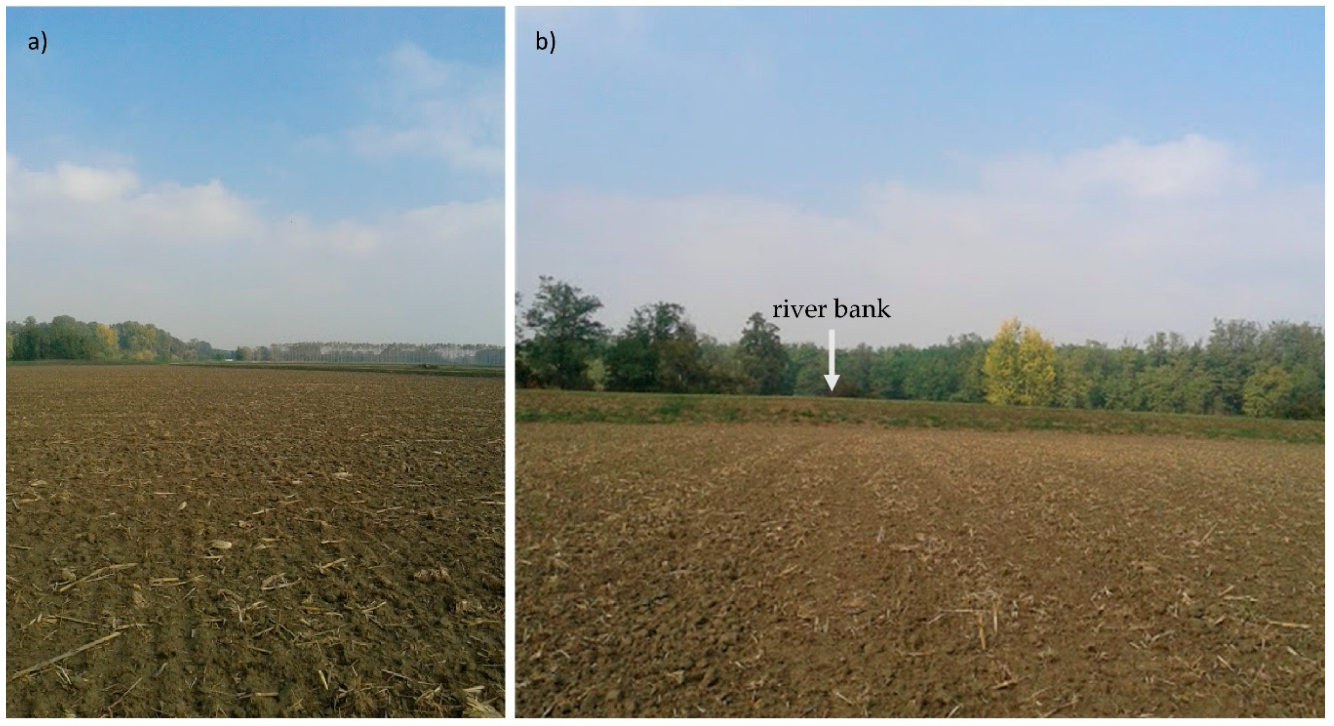
2.1. Study Area

The study was conducted in 36 field parcels (45.14° N, 9.28° E) of a total of about 195 ha, in a farm near Belgioioso town (Pavia, northern Italy, Figure 1). The parcels are situated on alluvial deposits on the left side of the Po River Valley, the main Italian river. In particular, they are subdivided in two blocks, the southern and the largest (173.5 ha) is situated on the actual alluvial plain (58 m a.s.l.) and it is characterized by fine flood deposits alternating to meandering channels with a sandy texture. The arboreal belt and riverbank, about 2 m high, separate the river from the crop fields (Figure 2). The northern block (21.5 ha) is situated in a river terrace, 15 m higher than the actual plain (around 73 m a.s.l.). It is characterized by fluvio-glacial deposits of the last glaciation (around 23,000 years B.P.), with a sandy texture and rare gravel lenses.

On average, long term (1981–2010) precipitation data shows an average of 830 mm∙year⁻¹ and average annual temperature of 13.5 °C. The cropping system of the fields is typical for this area, and is based on the rotation of corn (Zea mays L.), soybean (Glycine max (L.) Merr.), and sorghum (Sorghum bicolor (L.) Moench) in some cases.

Agronomic management was comparable in all studied fields. It was based on reduced tillage made by rotary disk-harrow and organic fertilization using the digested residue of biogas production (livestock manure, maize and sorghum). The amount of digested fertilizer varied from 50 to 80 m³∙ha⁻¹, according to nitrogen concentration. On average, about 150 kg∙ha⁻¹ of total nitrogen was supplied to the soil by digested fertilizer. Weed control is made through a pre-emergent chemical herbicide and post-emergent mechanical weed control. Water is mainly applied by furrow irrigation, although drip irrigation is also used for maize cultivation in seven fields. To verify the effect of irrigation typology on crop yield, a one-way ANOVA was tested, using drip/furrow irrigation as the categorical factor and crop yields (2016–2018) as dependent variables.

2.2. Proximal Sensing and Soil Mapping

The experimental fields were surveyed by an electromagnetic induction sensor system, mounted on a dedicated non-metallic sledge, named EMAS (electromagnetic agro-survey), developed by SO.IN.G s.r.l. (Livorno, Italy). The sensor includes a transmitter coil and three coplanar receiver coils, calibrated to survey the soil electrical resistivity (ER, in Ω∙m) at three pseudo-depths of about 0–50 cm, 0–100 cm, and 0–180 cm. The EMAS system was pulled by an all-terrain vehicle (quad) and included a global navigation satellite system (GNSS) and a dedicated rugged control unit to merge ER with geographic attributes for real-time viewing and saving. The survey was carried out in two consecutive days in low amounts and low spatial variability of soil moisture. The ER datapoints surveyed were interpolated by ordinary kriging, after semivariogram modelling.

Thirty-six calibration points (about one every 5 ha) were selected to cover the maximum spatial variability of the ER maps and elevation, obtained by the official DEM of the Lombardy region at a resolution of 5 m × 5 m (a CC file provided by cartographic services of Lombardy Region updated to 2015). The calibration points were sampled and described by manual auger. The soil was subdivided into horizons and described following the FAO official methods [32]. The topsoil horizons (A and B1 horizons) were collected for standard laboratory analysis, following the Italian official methods [33,34]. In particular, coarse fragments (>2 mm) were determined after dry sieving; texture was determined using the pipette method [35] and three granulometric classes (sand, silt, and clay); pH and EC were determined in a 1:5 water solution; total calcium carbonate was determined by Dietrich–Fruhling calcimeter; total soil organic carbon and total nitrogen were analyzed by dry combustion on an elemental analyzer; assimilable phosphorous by Olsen method, and cation exchange capacity (CEC) and total bases saturation (TBS) were analyzed using sodium acetate solution. Topsoil (0–30 cm) carbon stock (CS₃₀) was calculated following Intergovernmental Panel on Climate Change (Land Use, Land Use Change and Forestry) IPCC-LULUCF guidelines [36], using soil organic carbon, bulk density and coarse fragments as input variables. The soil available water capacity (AWC) was calculated by the pedotransfer function of Saxton and Rawls [37], using Soil Water Characteristics software.

The soils of all the calibration points were also classified using WRB 2014 [38] and correlated to the soil typological units (STUs) of the soil information system (scale 1:50,000) of the Lombardy region [39]. The STU map of the study area was obtained through a digital soil mapping approach. A support vector machine (SVM) classification was performed using the maps of electrical resistivity (ER1, ER2 and ER3) and the DEM (5 m × 5 m) as informative layers and the 36 calibration points, classified in the STUs, to calibrate the model. The procedure was carried out by SAGA-Gis, which implemented the model of Chang and Lin [40]. The average costs of highly-detailed soil surveys, comparable with the approach used for this work, were estimated for different survey extent by a market survey of some Italian companies that provide such services.

2.3. Yield Data

A precision-chop forage harvester (model: Krone BigX850, Germany) with a maize header was used to harvest silage maize from the field. A combined harvester (odel: Case 8320, USA) with a 7.5 m header was used to harvest soybean and sorghum. Both harvesters were used with a silage wagon supplied with load cells to monitor the variation of wagon weight instantaneously. A capacitance moisture sensor (Agrichem Inc., Ham Lake, MN, USA) was mounted along the travel path from the harvester to wagon, to monitor the moisture content of the harvested material.

Harvesters were supplied with a GNSS receiver with sub-metric precision. A handheld PC, mounted on the harvester cab, was used for data acquisition. The measured variables were coordinates, harvester speed, engine rpm (revolutions per minute), yield per second, and moisture content. A dedicated software allowed to calculate dry yield per hectare (Mg∙ha⁻¹) using yield per second and moisture content.

Defective observation and technical errors were removed from the yield dataset to ensure a satisfactory data quality. These technical errors have been largely documented in the literature [41] and they can be summarized as:

Harvester operator technical errors, including speed variation, overlapping of harvest passes, not fully using the cutting bar, etc.;

-

Harvester turns at the end of a harvest pass and headlands in a non-square field, where it is almost impossible to avoid overlapping harvest strips;

-

Accuracy of the positioning system and eventual offset between the true location of a yield observation and the coordinates recorded by the GNSS;

These measurement errors were manually removed from the yield dataset by the GIS. Overlapping passes, harvester turns, and machine speeds out of the average range (4–6 km∙h⁻¹) were removed from the datasets. Once the dataset of each year (2016–2018) and each crop typology (silage maize, soybean, and sorghum) were corrected, they were interpolated by ordinary kriging by geostatistical analysis in ArcGis 10.0. We decided to use the same model parameters to uniform all the interpolations. In particular, a spherical model was used, with a major range = 200 m, lag size = 20 m, and number of lags = 10.

2.4. Statistical Analysis

Preliminary investigations of the statistical relationships among yield variation (ΔY), soil features, elevation (h), and soil electrical resistivity (ER) were made by Pearson’s correlation, using the calibration points. To investigate multivariate correlations between ΔY and soil variables, a Principal Component Analysis (PCA) was calculated. ΔY was used as supplementary variable, which was not included in the calculation of PCA, but was plotted in the factor loadings graph according to the correlation with the PCA factors.

A forward stepwise multiple linear regression (MLR) was also tested between ΔY, as dependent variable, and the soil features with the highest and significant Pearson’s coefficients (r). To select variables that produced a significant improvement to the regression, an “F-to-enter” of higher than 10 was imposed during the stepwise process. Two clear outliers were removed from the dataset and then the MLR was recalculated.

Significant differences between STUs, in terms of ΔY and CS₃₀, were tested using one-way ANOVA and Fisher’s LSD test. Statistical analysis was performed by Statistica 8 data analysis software system (StatSoft Inc., Tulsa, OK, USA).

2.5. Economic Land Evaluation (Biomass Production, Carbon Sequestration and Flood Risk)

Economic evaluation of a land parcel should be computed considering the mean land market value (LMv) of that area and the site-specific deviations. This includes positive deviations due to site added values (i.e., a higher soil quality than average), and negative deviations due to disadvantages (i.e., high flood risk, a lower soil quality than average). In Italy, the official LMv is published by each province and used for expropriation procedures, according to national law D.P.R 327/2001 [42]. Land characteristics, like distance from the urban areas and roads, as well as the shape and size of the fields, were not considered during this work. These parameters are normally used for conventional land economic evaluation, therefore the method is already known and regulated.

In this work, site-specific deviations were calculated considering three important land features using the spatial geometries of the intersections between STUs and management units (or land parcels): (i) biomass production; (ii) carbon sequestration; and (iii) flood risk. The 36 calibration sites were used to study the relationships between the STU and associated functions, namely the mean yield variation (ΔY) and carbon stock of the topsoil (0–30 cm, CS₃₀). The latter is calculated following the official IPCC methods [35], which uses the SOC, bulk density and coarse fragment content.

Statistical correlation between the soil features and ΔY of the three years were calculated. ΔY in each calibration point (x) was calculated as:

$${\mathsf{\Delta }\mathrm{Y}}_x=\frac{1}{n}{\displaystyle \sum }_{i=0}^n\left(Y_{c,x}-\left|Y_c\right|\right)\times 100$$

(1)

where n is the number of years (two or three) with yield data, Y_c,x is the yield of each specific crop in the point x, $\left|Y_c\right|$ is the mean yield of the crop in all the surveyed fields. This equation allows for the standardization of the yield for crop typology and year. The limit of this calculation was the use of the mean yield ($\left|Y_c\right|)$ based only on this farm, and not on the average yield of the province, where the LMv was calculated. Unfortunately, the average yield at the provincial scale is discontinuous and, in some cases, not available. In the following chapter, we reported the available regional data, only for comparison with the farm average data. Where the local/regional yield data is available, they should be used to calculate the ΔY.

Variations of the productive value of a land (ΔY_V), which represent the local variation of land value related to the variation of biomass production, was determined using the concept of capitalization rate (CR). CR is defined as the ratio between the average gross saleable production (GSP) of the crop yield and the mean land value (LMv). The latter is defined as:

$$CR=\frac{GSP}{LMV}$$

(2)

In Italy, the mean GSP per hectare of most of the crops was reported by the national Farm Accountancy Data Network [43]. Using this mean CR, it is possible to calculate ΔY_V of each STU due to the variation in the gross saleable product, following:

$${\mathsf{\Delta }\mathrm{Y}}_v=\frac{GSP\times \mathsf{\Delta }\mathrm{Y}}{CR}$$

(3)

Local variation in the carbon stock value (ΔCSv, €∙ha⁻¹) of each STU was calculated multiplying the CS₃₀ deviation (ΔCS₃₀) from the local mean (|CS₃₀|), the mean annual EU allowance price relative to the calendar year preceding the value estimation (EUA_y) and the ratio of CO₂ and carbon molecular weights (=3.66).

$$\mathsf{\Delta }\mathrm{CSv}={\mathsf{\Delta }\mathrm{CS}}_{30}\times 3.66\times EU{A}_y$$

(4)

The mean CS₃₀ for the agrarian zone “Basso Pavese”, Pavia province, where the study is located, was calculated using the Global Soil organic Carbon Map (GSOC), recently published by FAO and ITPS [44]. The polygon of the “Basso Pavese” agrarian region was used for the extraction of the CS₃₀ mean from the GSOC map. Similar to biomass production, the site-specific ΔCSv was expressed as a variation in relation to the average “Basso Pavese” CSv.

The flood risk of each parcel was determined according to the Lombardy regional map of flood risk, which follow the EU flood directive 2007/60/CE. A farmer interview was also done to confirm and improve the flood risk of the area. Although the Lombardy region realized a plan of Flood Risk Management (PGRA), in accordance with the flood EU directive, the flood risk in agricultural areas along the river is still elevated. To determine the land value variation due to the different flood risk, some assumptions must be done. Potentially, a flood can damage the whole annual crop yield, but it is strongly dependent on the period and duration of the flood event, coupled with the crop typology and its phenological phase during the event. When the flood risk is elevated (about five flood events every 100 years), we assumed that, at least once, the farmer will have a complete damage of crop yield, and then the loss of annual GSP. Moreover, land levelling and tillage to recover a field after flooding has a cost. Such cost was estimated on the basis of Italian official fares for agricultural works, subdivided for the Province, published by agricultural third-party workers [45]. The flood risk costs (FRc), calculated adding the annual GSP of each STU with the land recovery costs, should be subtracted from the LMv in elevated flood risk areas.

Finally, the variation of land mean value (ΔLMv), based on the spatial variability of soil typological units, and then functions (ΔYv: variation of productive value of a land; ΔCSv: variation of carbon stock value), as well as flood risk costs (FRc) was calculated as follows:

$$\mathsf{\Delta }\mathrm{LMv}=\mathsf{\Delta }\mathrm{Yv}+\mathsf{\Delta }\mathrm{CSv}-\mathrm{FRc}$$

(5)

The values of ΔLMv, calculated for each STU, was interpolated following the STU map, obtaining a map of land value variation based on soil spatial variability. The land value per hectare of each land parcel was calculated adding its internal ΔLMv mean to the LMv.

3. Results

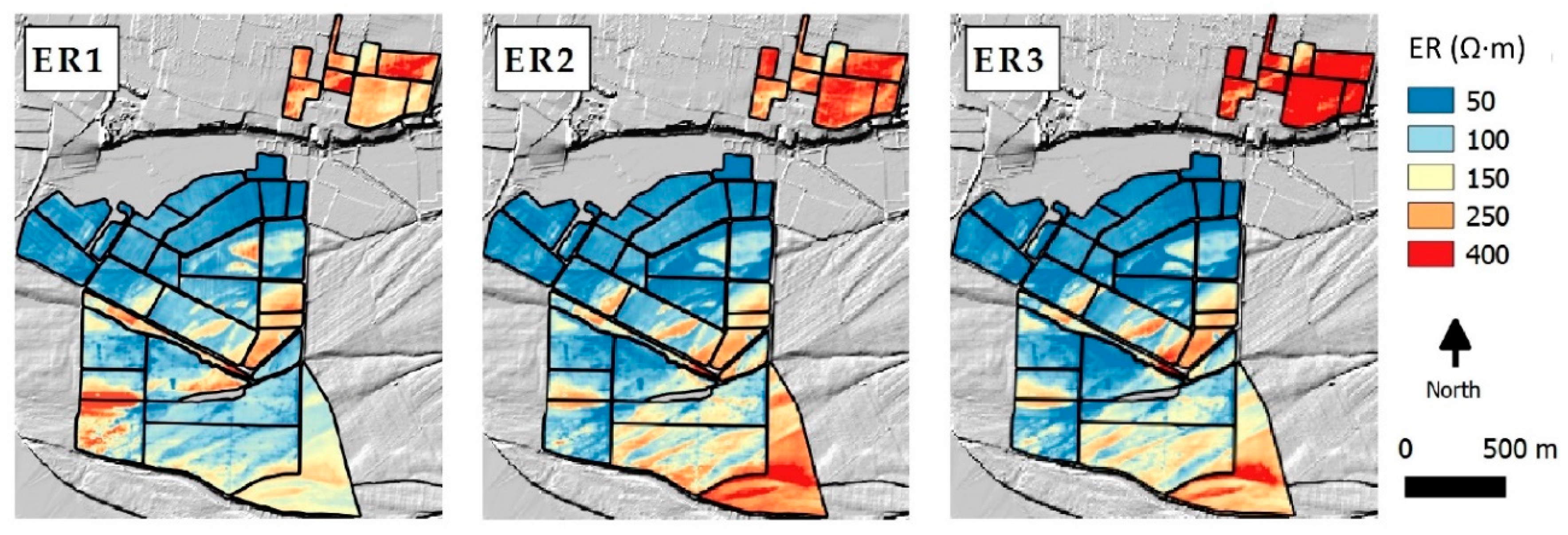
3.1. High Detail Soil Mapping by Proximal Sensing

The topsoil electrical resistivity (ER1, about 0–50 cm) ranged between 10 to 520 Ω∙m, whereas ER2 (about 0–100 cm) between 15 and 550 Ω∙m and ER3 (about 0–180 cm) between 15 and 1000 Ω∙m. In general, the northern block showed a higher ER, because of their coarser texture (sandy loam or sandy) than the southern block (Figure 3). In the southern block, ER values higher than 100 Ω∙m corresponded to lenses of alluvial loamy sand material of old meandering channels and fluvial bars. Other meandering forms in the central part of the southern block showed the lowest ER values (from 10 to 50 Ω∙m), related to a generally finer texture (silty loam). The 36 calibration points, selected to cover the maximum ER variability, were investigated by soil description and analysis of manual augerings (

Table 1. Descriptive statistics of proximal sensing and data of soil typological units (PES1 and PES3: Peschiera1 and 3, PCH1: Porta Chiozza1; GIA: San Giacomo, ISN: Isolone units). CF: coarse fragments, CaCO₃: total calcium carbonate, SOC: soil organic carbon, TN: total nitrogen, CEC: cation exchange capacity, TBS: total base saturation, AWC: available water capacity, ER: soil electrical resistivity.

	hor.	Depth	Sand	Silt	Clay	CF	pH	CaCO3	SOC	TN	CEC	TBS	AWC	ER1	ER2	ER3
		(cm)	(%)					(g kg−1)			(meq∙cm−1)	(%)	(cm3∙cm−3)	(Ω∙m−1)
PES1 (n = 6)	Ap	41	74	20	6	5	6.8	0.0	17.1	1.89	11.9	50	0.09	216	200	332
	C	74	70	27	3	7	-	-	-	-	-	-
PES3 (n = 3)	Ap	40	89	7	4	3	7	11	11.6	1.4	8.4	52	0.06	366	380	939
	C	100	78	21	1	4	-	-	-	-	-	-
GIA (n = 9)	Ap	39	36	50	14	0	8.3	12	7.0	1.18	14.4	82	0.16	94	87	96
	Bw	88	58	36	6	0	-	-	-	-	-	-
ISN (n = 10)	Ap	40	7	70	23	0	8.3	31	9.1	1.45	16.9	89	0.20	86	82	76
	Bw	91	10	72	18	0	-	-	-	-	-	-
PCH1 (n = 8)	Ap	39	58	35	7	0	8.4	7.0	5.7	0.91	11.3	71	0.11	206	208	227
	Bw	97	71	25	4	0	-	-	-	-	-	-

). Five different soil typological units (STUs) were recognized and correlated to the regional soil units of the Lombardy soil information system [38]. The pinpointed STU are:

-

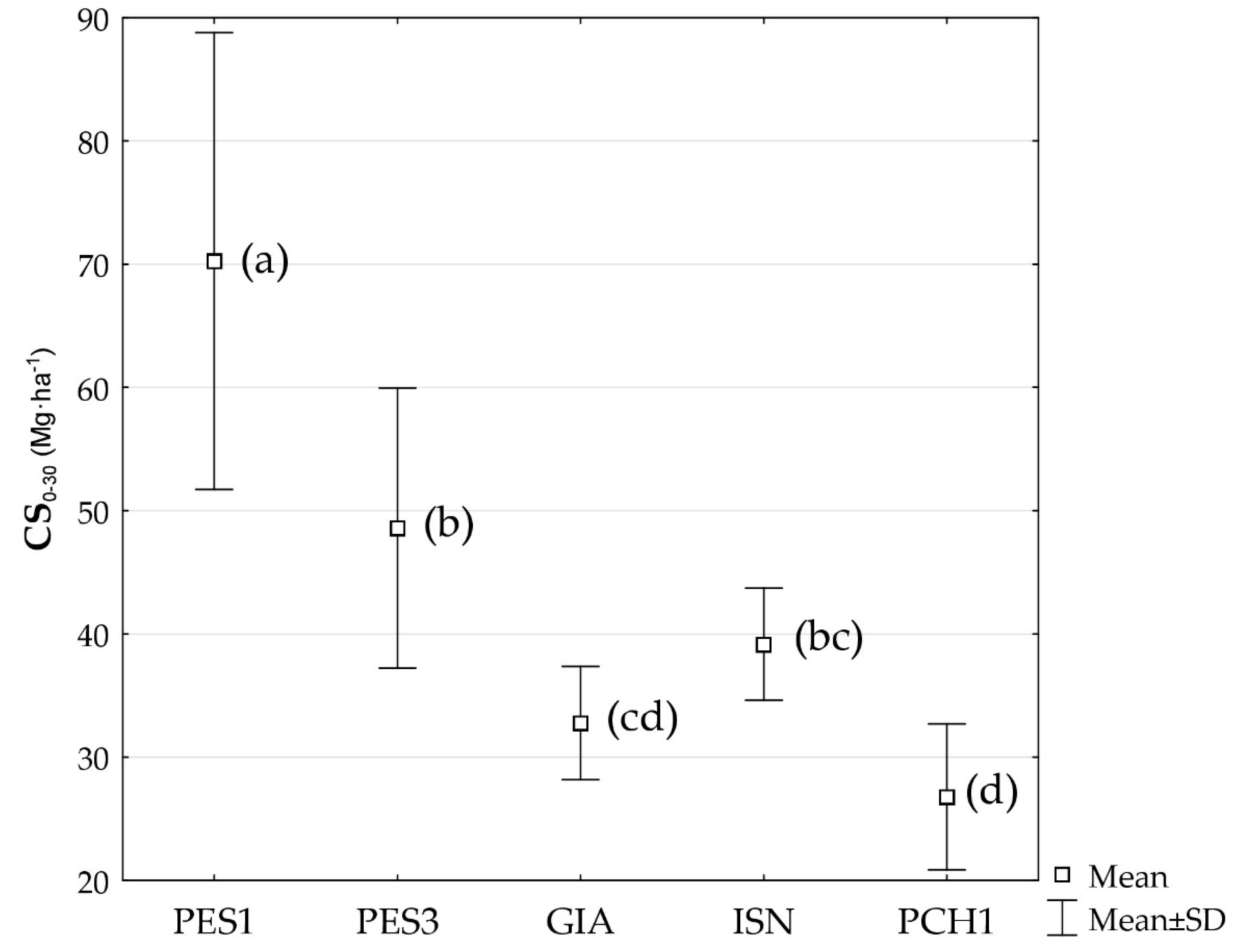
GIA (San Giacomo unit): brown soils on fluvial overflow deposits, characterized by an Ap-Bw-C horizon sequence, silty loam, without coarse fragments, slightly calcareous, poor in organic matter, classified as Calcaric Fluvic Cambisol (Siltic).

-

ISN (Isolone unit): pale brown soils on fluvial overflow deposits, characterized by an Ap-Bg-C horizon sequence, silty loam with a lower sand percentage than GIA, without coarse fragments, slightly calcareous, poor in organic matter, with moderate waterlogging of subsoil horizons (B or C), classified as Calcaric Endogleyic Cambisol (Siltic).

-

PCH1 (Porta Chiozza unit): pale brown soils on sandy alluvial lenses, characterized by an Ap-C horizon sequence, sandy loam (sometimes sandy in the subsoil) without coarse fragments, very poor in organic matter, classified as Calcaric Fluvisol (Arenic).

-

PES1 (Peschiera1 unit): dark brown soils on old fluvial terrace, characterized by an Ap-Bw-C horizon sequence, loamy sand with scarce coarse fragments, non-calcareous and sub-acid, moderately rich in organic matter, classified as Dystric Fluvic Cambisol (Arenic).

-

PES3 (Peschiera3 unit): brown soils on paleochannels of old fluvial terrace, characterized by Ap-C horizons sequence, sandy with scarce coarse fragments, neutral pH and moderate organic matter, classified as Eutric Fluvisol (Arenic).

The STU map was obtained by Support Vector Machine (SVM) classification, following the method described above. In the northern block, PES1 and PES3 cover almost the total area of the experimental fields, and only a small part (and a calibration point) is attributed to a GIA unit. In the southern block, most of the area is covered by GIA and ISN units, whereas some lenses of PCH1 are frequent in the southern part of the block, closer to the Po River (Figure 4).

The costs of the survey are dependent on the total extent of the investigation. From a market survey, we calculated from about 300 €∙ha⁻¹ for small extensions (10–30 ha) to about 100 €∙ha⁻¹ for areas larger than 500 ha (Figure 5). In general, soil mapping is valid for many years unless there has been significant land movement. Although the organic matter, pH and nutrient content could vary year after year, mainly because fertilization, soil spatial distribution remains over the years.

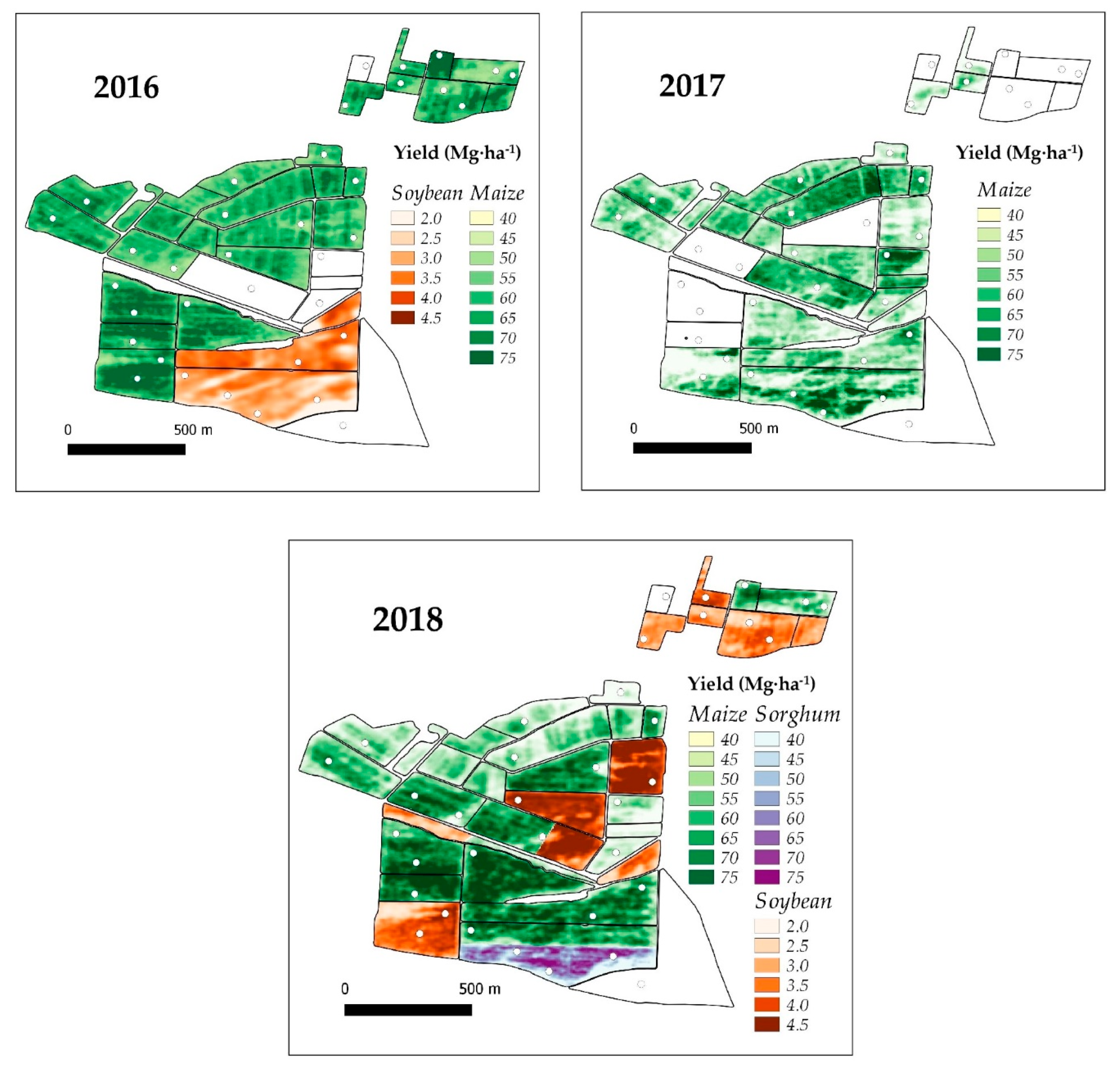
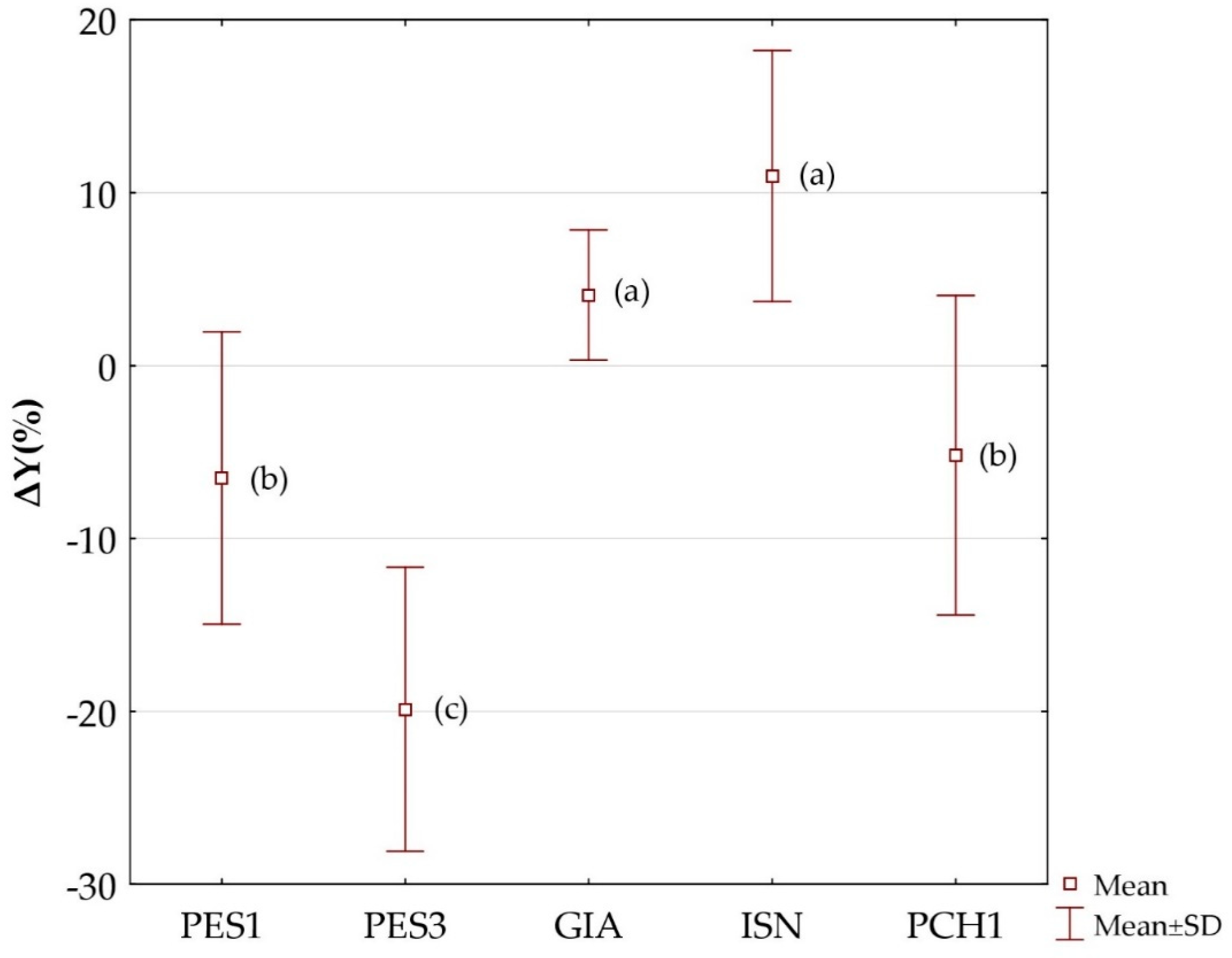
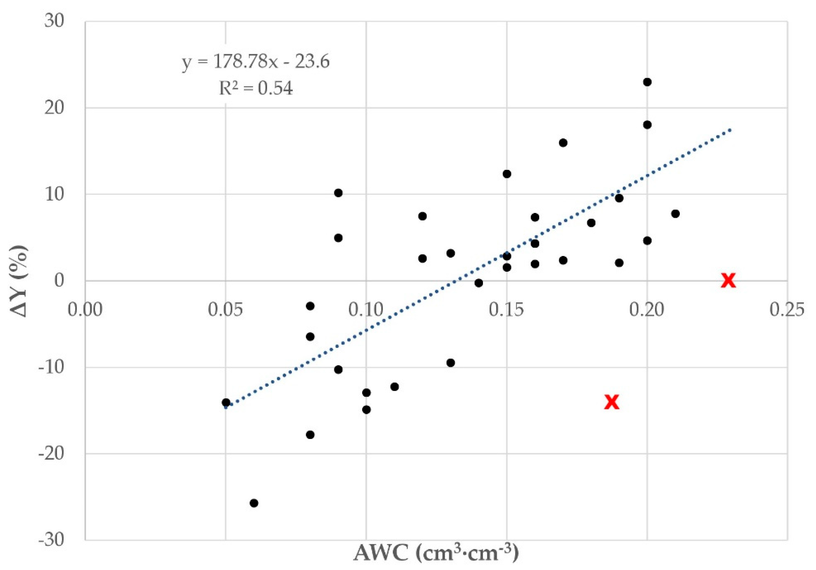
3.2. Crop Yield Mapping and Standardized Yield Variation

All the crop yield data of the three years (2016, 2017, and 2018) and three crop typologies (silage maize, soybean and sorghum) needed to be corrected for technical errors of measurements. In particular, speed variation, overlapping passes and harvester turns were the most common errors and removed from the dataset.

Table 2. Descriptive statistics of the yield maps. ¹: Standard deviation; ²: Root mean square error of kriging; ³: mean crop yield at regional scale, published by regional Directorate-General Agriculture (www.regione.lombardia.it).

	Year	Surface	Mean	SD 1	RMSE 2	Regional Data 3
		ha	Mg∙ha−1
Silage Maize	2016	93.2	62.3	7.7	6.1	55.8
	2017	80.5	52.9	10.1	8.3	50.4
	2018	86.3	63.4	11.2	9.3	n.a.
Soybean	2016	12.8	3.0	0.6	0.4	4.1
	2018	79.8	3.6	0.7	0.5	n.a.
Sorghum	2018	4.0	55.0	11.8	9.4	n.a.

showed the descriptive statistics of the maps and the root mean square error (RMSE) of the ordinary kriging. The RMSE is high because of the elevated short-range variability of the yield datapoints, mainly due to measurement outliers and technical errors of measurement, which cannot be corrected. The interpolation of yield data, using a wide lag size, allowed for the smoothing of eventual outliers, obtaining yield maps of fair quality to understand yield spatial variations and relationships with soil spatial variability (Figure 6). In 2016, most of the available yield data referred to silage maize (93.2 ha) and with a small amount of data on soybean (12.8 ha). In 2017, only the silage maize yield was available, whereas in 2018 the silage of maize, soybean, and a field cultivated with sorghum were available (Table 2). On average, the silage maize yield is between 62 and 63 Mg∙ha⁻¹, although in 2017 was lower (52.9 Mg∙ha⁻¹). The official regional data reported similar mean yields of silage maize, which were 55.8 Mg∙ha⁻¹ in 2016 and 50.4 Mg∙ha⁻¹ in 2017 (Table 2). The soybean yield was a little higher in 2018 (3.6 Mg∙ha⁻¹) than 2016 (3.0 Mg∙ha⁻¹), whereas the mean sorghum yield in 2018 was 55 Mg∙ha⁻¹. Regional data of soybean mean yield was reported only in the 2016 data, which was 4.1 Mg∙ha⁻¹. No statistical differences in crop yield were shown between the fields with drip irrigation and furrow irrigation, after one-way ANOVA analysis.

The standardized mean yield variation (ΔY) was calculated in all the calibration points, except two points that had no yield data or data only for one year. ΔY varied between −25.7% and +23%, with a distribution close to normality, since the Shapiro–Wilks’s test satisfied the null-hypothesis (W = 0.97, p = 0.37).

Analysis of variance (one-way ANOVA) using STU as grouping factor, showed a significant effect of soil typology on crop yield (F = 11, p < 0.0001). In particular, Fisher’s LSD test showed three homogeneous groups (significant for p < 0.05) for ΔY (Figure 7). The highest positive values of ΔY belonged to ISN and GIA (from +4 to +11%, on average), whereas the most negative values belonged to PES3 (−19.8%). PCH1 and PES1 showed slightly lower ΔY than the average (−5.2 and −6.5, respectively).

Analyzing the single calibration points, ΔY showed high positive correlations with AWC, silt fraction and CEC, and negative correlations with sand (significant for p < 0.01,

Table 3. Pearson’s correlation between the mean yield variation (ΔY), elevation (h), electrical resistivity (ER1, ER2, ER3) measured by proximal sensing and soil features (CF: coarse fragments, AWC: available water capacity, TN: total nitrogen, SOC: soil organic carbon, CEC: cation exchange capacity, TBS: total base saturation, P: assimilable phosphorus). The AWC was calculated by a pedofunction which used clay, sand, CF, and bulk density as input data (Saxton and Rawls, 2006). In bold, values significant for p < 0.01.

	ΔY	h	ER1	ER2	ER3
h	−0.33
ER1	−0.59	0.66
ER2	−0.61	0.66	0.89
ER3	−0.62	0.75	0.88	0.93
AWC	0.60	−0.67	−0.72	−0.74	−0.72
CF	−0.39	0.58	0.36	0.39	0.44
Sand	−0.53	0.70	0.74	0.76	0.73
Silt	0.56	−0.71	−0.72	−0.74	−0.73
Clay	0.33	−0.57	−0.68	−0.68	−0.63
pH	0.35	−0.82	−0.46	−0.53	−0.60
SOC	−0.06	0.71	0.15	0.25	0.32
TN	0.03	0.55	−0.01	0.05	0.16
CaCO3	0.22	−0.45	−0.43	−0.43	−0.39
CEC	0.51	−0.46	−0.72	−0.74	−0.66
TBS	0.42	−0.74	−0.62	−0.65	−0.64
P	−0.17	0.76	0.49	0.49	0.51

). The multivariate approach, which uses principal component analysis (PCA), confirmed strong relationships between ΔY and AWC, clay, CEC and TBS.

A linear regression between ΔY and AWC, which was the soil parameter with the highest statistical relationship with ΔY, was calculated (Figure 8). The coefficient of determination (R²) referred to 34 data-points was low (0.38), mainly because of only two outliers. Removing the two outliers, linear regression strongly improved, showing R² = 0.54 (p < 0.001) and standard error of estimation (SE) of 7.54.

CS₃₀ mean of the “Basso Pavese” agrarian region, extracted by the GSOC map [44], was 50.35 Mg∙ha⁻¹. PES1 showed CS₃₀ positive deviation of 19.9 Mg∙ha⁻¹, whereas the other STUs showed lower CS₃₀ than the average (Figure 9). In particular, PCH1 showed the lowest value, which was 23.6 Mg∙ha⁻¹ lower than the average of the agrarian region.

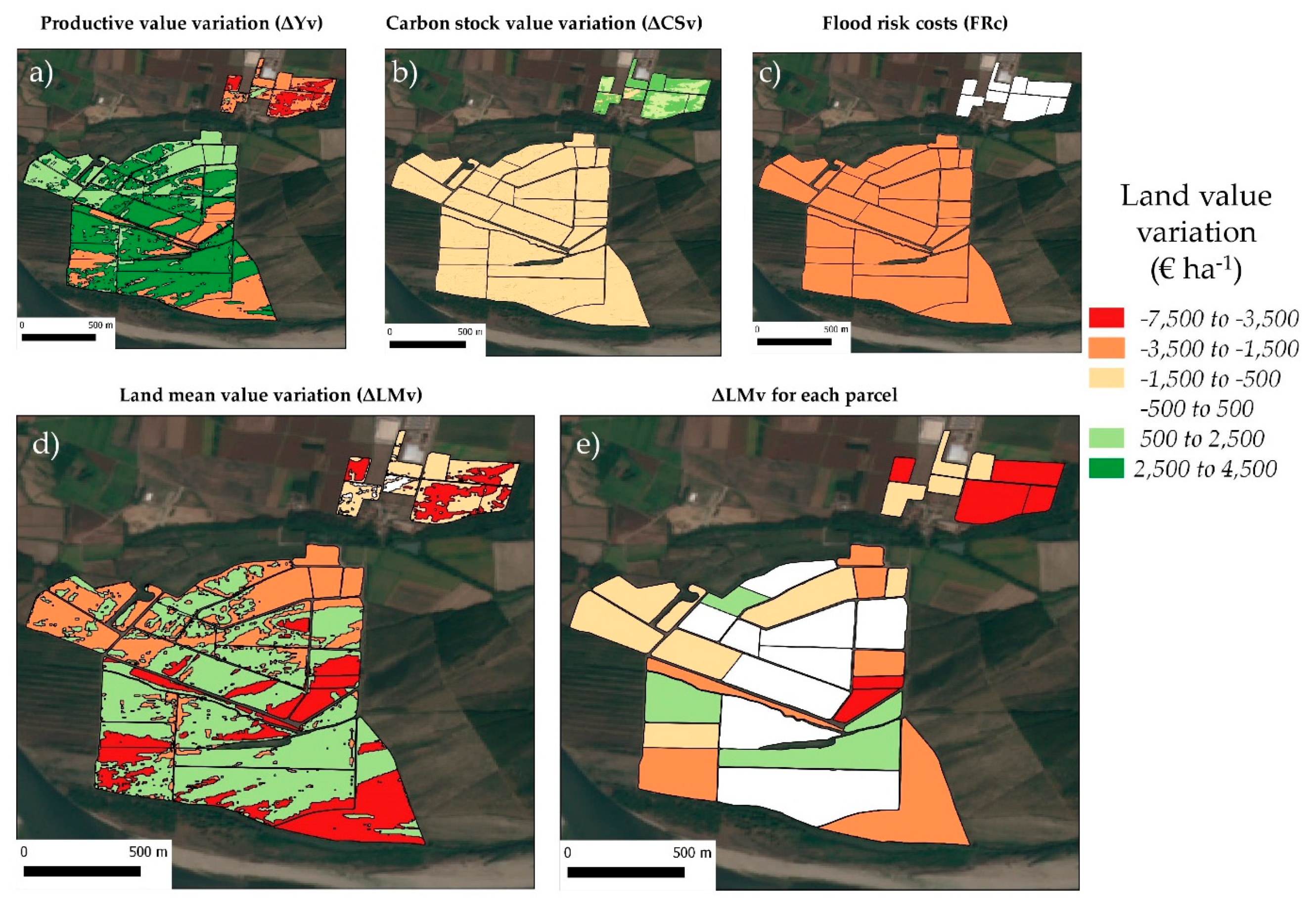
3.3. Economic Evaluation

LMv of irrigated cropland parcel in the studied area (Pavia province, agrarian zone n.11 “Basso Pavese”, formed by 17 municipalities) was 37,000 €∙ha⁻¹ (updated to 2018).

In the Lombardy Region, the mean official GSP of the two most representative crops, silage maize and soybean, updated to 2013, are 1672 and 1565 €∙ha⁻¹, respectively. Therefore, the GSP in this agricultural system can be estimated 1619 €∙ha⁻¹, on average. Then, the mean CR of this agricultural system is:

$$CR=\frac{1619}{\mathrm{37,000}}=4.4\%$$

Once the ΔY was calculated for each STU, as explained in the previous chapter, the variation of land value due to biomass production function (ΔY_V) was computed using Equation (3). The GIA and ISN STUs were more productive than average, as demonstrated in the previous chapter, therefore their ΔY_V showed positive values of +1508 and +4038 €∙ha⁻¹, respectively (

Table 4. Economic land evaluation based on STUs (PES1 and PES3: Peschiera1 and 3, PCH1: Porta Chiozza1; GIA: San Giacomo, ISN: Isolone units). ⁽¹⁾: mean yield variation from the local average, standardized for crop typology and year; ⁽²⁾: variation of carbon stock (0–30 cm) from the local mean (50.35 Mg∙ha⁻¹); ⁽³⁾: variation from the local average of annual gross saleable production; ⁽⁴⁾: variation of productive value of a land, calculated by eq. (3); ⁽⁵⁾: variation of the land value due to different soil carbon stock; ⁽⁶⁾: costs of flood risk, calculated using the loss of one year GSP of each STU plus fixed land recovering costs (300 €∙ha⁻¹). FRc was applied only in elevated flood risk areas (southern block), individuated by regional flood risk map.

STU	ΔY(1)	ΔCS(2)	ΔGSP(3)	ΔYv(4)	ΔCSv(5)	FRc(6)
	(%)	(Mg∙ha−1)	(€∙ha−1)
PES1	−6.5	19.9	−105	−2390	1162	−1813
PES3	−19.8	−1.8	−320	−7281	−102	−1598
PCH1	−5.2	−23.6	−84	−1912	−1376	−1834
GIA	4.1	−17.6	66	1508	−1026	−1984
ISN	11.0	−11.2	178	4038	−653	−2096

). On the contrary, the STUs characterized by lower yields than average, namely PCH1, PES1, and PES3, showed negative ΔY_V of −1912, −2390, and −7281 €∙ha⁻¹.

Elaborating on the carbon price viewer [28] EUA₂₀₁₈ resulted 15.95 €/Mg CO₂. The “Basso Pavese” CS₃₀ estimated by FAO GSOC map resulted 50.35 Mg∙ha⁻¹. Therefore, the mean CSv of studied area resulted 2939.28 €∙ha⁻¹. The ΔCSv for each STU is reported in Table 4.

The northern block of the study area has an absent flood risk, whereas the southern block shows an elevated flood risk, with a frequency of an event every 20 years. According to farmer interviews, the floods in most of the fields of southern block are indeed more frequent, but total loss of production effectively occurred about once every 20 years. Complete loss of crop yields due to floods corresponded to the economic value of GSP. Regarding the cost estimation of land recovery after flooding, the cleaning and the restoration of the field channels (50 € ha⁻¹), removal of accumulated materials and land levelling (100 €∙ha⁻¹), shallow tillage and seed bed preparation (150 €∙ha⁻¹) were considered. Therefore, the total costs estimation for land recovery after every flood was 300 €∙ha⁻¹.

From these criteria, the total economic cost of flood risk (FRc) was estimated adding costs for land recovery to the GSP value of one year for each STU, and then varied between −1598 €∙ha⁻¹ in PES3 to −2096 €∙ha⁻¹ in ISN, because of higher annual GSP. The FRc was added to the ΔLMv only in the southern block, because the regional flood risk map reported elevated risk for this area (greater than five events every 100 years). The northern block showed no flood risk, therefore the FRc was not taken into account for the ΔLMv calculation.

The ΔLMv map was the result of adding the ΔYv, ΔCSv and FRc. The ΔLMv was also calculated for each land parcel, providing the corrected land value of each parcel (Figure 10). The parcel ΔLMv vary between −5560 and +1100 €∙ha⁻¹. Most of the parcels showed values comparable with the LMv (−500 to +500 €∙ha⁻¹), or slightly lower (−1500 €∙ha⁻¹). Only six parcels showed a land evaluation about 4000–5560 €∙ha⁻¹ lower than the LMv. These parcels were mainly characterized by soils with evidently lower potential yields than average (PES1, PES3, PCH1). Only four parcels showed higher land values than average (+500 to +1100 €∙ha⁻¹), mainly due to the high potential productivity of their soils (mainly ISN). The lower CS than average and the costs due to flood risk, make the increase of land value of these parcels limited, although the potential yield was higher than average.

4. Discussion

The proximal EMI soil survey, coupled with few soil descriptions and analysis, allowed an accurate map of soil typologies (STUs) and their associated functions to be obtained. As described in the previous chapter, the costs for the highly-detailed soil survey carried out during this work can vary between 100 and 200 €∙ha⁻¹ for total surfaces wider than 100 ha (Figure 5). Such costs should be paid only once, since the maps of soil spatial variability obtained from this survey can be considered stable over the years. The method of this work was based on EMI proximal survey, but it is possible to obtain greater detail soil maps for precision land evaluation through other methods. In the literature, several examples of highly-detailed soil mapping with innovative techniques are reported, most of which use other proximal soil sensors, like gamma-ray spectroscopy [21,46] and Vis-NIR diffuse reflectance [47,48,49]. The use of remote sensing methodologies, from satellite to drone (UAV), was also reported in the literature to obtain detailed maps of soil features [50,51]. Other works used a digital elevation model and its covariates with computational methods, like artificial neural networks or support vector machines, to obtain high-detail soil maps [30]. The latter are more suitable for landscapes with important landforms, like slopes, depressions, and terraces, but not in plains, as in the present work.

In this research, five STUs were individualized, which diversified them for sedimentary processes as well as pedogenesis. ISN and GIA were both characterized by their fine texture, due to the deposition of fluvial overflows. ISN showed the highest clay content (around 20%), which tended to increase water and nutrient availability (high AWC and CEC). This can be considered the most fertile soil of the studied area, and indeed showed the highest mean yield (+11%, on average). GIA showed a generally lower AWC and CEC than ISN, and was also associated with a slightly lower yield. In the actual alluvial plain, PCH1 was the soil derived by flood paleochannels, characterized by a texture coarser than ISN and GIA. This STU showed clear lower hydrological and chemical fertility, characterized by lower AWC, CEC, and base saturation, as well as mean reduction of crop yield (−5.2 % on average). SOC and TN content were low in all these quoted STUs, because the soils have been continuously renewed by fluvial floods (about five floods every 100 years) and intensively tilled for years.

In the upper fluvial terrace, corresponding to the northern block of the studied area, the two most representative soil units were PES1 and PES3. Only a small area was classified as GIA units. The deposits of this terrace showed higher sand content and SOC, as well as sub-acid pH, lower CEC and base saturation than the southern block. In these soils, the deposition of the parent material was earlier than the southern block, and the soils have not been renewed by recent fluvial floods. Although these soils showed higher SOC and TN content, the fertility and then biomass production was generally lower than the southern block. As a matter of fact, sandy texture restricted the soil water retention, as well as CEC, whereas higher organic matter and sub-acid pH tended to increase leaching and to reduce base saturation. In particular, PES3 had a sand fraction of more than 80% and 0.06 cm³∙cm⁻³ AWC and showed about a 20% decrease in the mean yield.

The statistical analysis showed no correlation between the SOC and yield, as well as between the TN and yield. In fact, drought stress can be only partially alleviated by an increase in the nutrient supply, specifically easy assimilable nitrogen (nitrate), which can regulate water flux through plants [52]. Therefore, in this agrarian landscape, higher SOC and TN did not imply higher biomass production. On the other hand, this study showed how both CEC and, in particular, AWC played the main role in biomass production of the reference crops (maize, soybean, and sorghum). The slope of the linear regression between ΔY and AWC (178.78, Figure 7) can be used to estimate the increase in yield, knowing the soil AWC. For instance, a 0.01 cm³∙cm⁻³ AWC increase leads to a 1.78% increase in yield; considering the mean GSP for this area (1619 €∙ha⁻¹), this small AWC increase potentially involves a 28.8 € ha⁻¹ GSP increase. Although this economic value could be valid only for these boundary conditions, namely irrigated croplands in the “Basso Pavese” agrarian zone, the positive relationship between yield and soil AWC has been often observed [19,53]. Moreover, economic quantification of soil AWC variation allows the valuing of practices that preserve and increase soil water retention. The AWC is strongly related to natural physical features like texture and coarse fragments, but it is also directly related to soil organic matter and porosity [37], which can be modified positively or negatively by human activity. Best-practice soil management can increase both soil organic matter and porosity, and then increase the AWC. Celik et al. [54] reported up to a 0.08 cm³∙cm⁻³ AWC increase after five years of compost application in Mediterranean soils. Bescansa et al. [55] reported a 0.03 cm³∙cm⁻³ AWC increase after five years of no-till management in relation to moulboard conventional tillage in northern Spain. Long-term experiments in the USA [53] confirmed the positive effects of no-till practices on soil AWC. In the Po River plain, Andrenelli et al. [56] reported soil AWC increases from about 0.02 to 0.03 cm³∙cm⁻³ after one-year treatment of pelletized biochar (14 Mg∙ha⁻¹) in silty clay loam soil. Applying the AWC-GSP correlation obtained in this study, the soil management practices reported from these papers can potentially have a positive effect on the GSP of 57 to 230 €∙ha⁻¹. Further studies should be done to improve and generalize the estimation of the economic impact of these soil best practices.

The economic evaluation of the biomass production functionality for each STU reported a wide range of values (Table 4). All sandy and sandy loam soils with AWCs lower than 0.11 cm³∙cm⁻³ and CECs lower than 12 meq∙cm⁻¹ showed lower yields than the local average, and then their productive economic values (ΔYv) varied between −1912 to −7281 €∙ha⁻¹, with the minimum value in the PES3 unit. On the other hand, PES STUs had higher carbon stocks than the local mean, and then their economic evaluation had to take in account this environmental value. This economical value is not only related to CO₂ sequestered by the soil, but also general increases in soil quality regarding biological activity, nutrient cycling, soil structure and ease of cultivation. As reported in the results paragraph, this case study showed an unusual yield decrease in STUs rich in SOC and TN, explainable with a stronger decrease of AWC and CEC due to their coarser texture. Examining this issue more deeply, the SOC in the least productive soil (PES3), was only 2.5 g∙kg⁻¹ higher than the highest productive soil (ISN), whereas its AWC was about one third (−0.10 cm³∙cm⁻³), and its CEC was about half of that in ISN. Then, in this study, SOC and TN spatial variability played a minor role on crop yield variation mainly due to soil texture. In general, when the origin of parent material and soil texture are similar, increases of SOC correspond to increases of CEC, nutrients, and water availability [57], and then potential crop yield, apart from organic soil like histosols (peats).

Eventually, the elevated risk of flood events in this landscape required an account for its economic impact. The frequency of flood risk can be obtained by regional maps, available in most of European regions, or by specific studies at higher detail. However, to take into account the flood risk in economic evaluations, few assumptions should be made. In elevated risk areas, where the flood return time is less than 20 years, it is assumable that a complete loss of crop yield and damages to land (erosion channels, deposition of material) could occur once during a farmer’s working activity. For this reason, the price of elevated flood risk areas should be discounted from the costs for land recovery and yield damage.

The final result of this work reported on the map of variation from mean land value (ΔLMv), calculated for each parcel (Figure 10e), according to internal STU spatial variability. The only productivity land value (ΔYv) that showed higher differences between the STUs than the final ΔLMv, was mainly because the highest productivity STUs (ISN and GIA) had lower CS₃₀s than the local average, and were in an elevated risk area. These negative conditions tended to slightly decrease the land value, limiting the economic differences between the southern and northern block, the latter characterized by a higher CS₃₀ and no flood risk.

Further studies should be done to quantify the farm scale economic impact of other soil ecosystem services, like water purification, contaminant reduction, and nutrient cycling [9,16,58]. These functions are strongly related to several soil features like soil texture, internal drainage, pH, CEC and microbial activity [58,59,60]. In prospect, policies should be taking into account soil spatial variability, and the effect of the different soil features. For example, the EU directive concerning the protection of waters against nitrate pollution from agricultural sources (Council Directive 91/676/EEC) actually does not consider soil features, but only the distance from aquifers, although many researchers have shown how different physical-hydrological soil characteristics can affect water purification function and contaminant reduction [61,62,63].

5. Conclusions

The methodology used in this work allowed for an assessment of the economic land evaluation at a high detail of irrigated croplands in the Po River Plain, taking into account the soil functions of biomass production and carbon stock, as well as land depreciation due to elevated flood risk. The results of this work showed that:

-

Soil features and their associated functions can strongly vary within a land parcel and, in general, within a farm.

-

This soil spatial variability should be taken into account during economic land evaluation, because the natural capital of the soil and the economic return due to biomass production follow this variability.

-

The approach proposed in this paper can be applied in many other lands, specifically croplands in alluvial plains. With the awareness that most of the needed data, like the LMV, GSP, mean CS₃₀, flood risk, etc., are usually available for developed countries.

Further studies should be done to assess the spatial variability of other soil ecosystem services, namely water purification, nutrient cycling and the biodiversity pool, and then to assess their economic value variation. The inclusion of criteria regarding farm-scale soil quality in policies could be foster the use of methodology to assess economic value of soil ecosystem services. Finally, the economic assessment could stimulate the interest of farmers to increase the functionality of their soils, by proper land management.

References

1. FAO. A Framework for Land Evaluation; Food and Agriculture Organization of the United Nations: Rome, Italy, 1976; Soil Bulletin 32; Available online: http://www.fao.org/3/x5310e/x5310e00.htm (accessed on 22 July 2019).
2. Rossiter, D.G. Economic land evaluation: Why and how. Soil Use Manag. 1995, 11, 132–140. [Google Scholar] [CrossRef]
3. Hoobler, B.M.; Vance, G.F.; Hamerlinck, J.D.; Munn, L.C.; Hayward, J.A. Applications of land evaluation and site assessment (LESA) and a geographic information system (GIS) in East Park County, Wyoming. J. Soil Water Conserv. 2003, 58, 105–112. [Google Scholar]
4. De la Rosa, D.; Mayol, F.; Diaz-Pereira, E.; Fernandez, M.; de la Rosa, D., Jr. A land evaluation decision support system (MicroLEIS DSS) for agricultural soil protection: With special reference to the Mediterranean region. Environ. Model. Softw. 2004, 19, 929–942. [Google Scholar] [CrossRef]
5. Manna, P.; Basile, A.; Bonfante, A.; De Mascellis, R.; Terribile, F. Comparative Land Evaluation approaches: An itinerary from FAO framework to simulation modelling. Geoderma 2009, 150, 367–378. [Google Scholar] [CrossRef]
6. Baveye, P.C.; Baveye, J.; Gowdy, J. Soil “ecosystem” services and natural capital: Critical appraisal of research on uncertain ground. Front. Environ. Sci. 2016, 4, 41. [Google Scholar] [CrossRef]
7. Halder, J.C. Land suitability assessment for crop cultivation by using remote sensing and GIS. J. Geogr. Geol. 2013, 5, 65–74. [Google Scholar] [CrossRef]
8. Haines-Young, R.; Potschin, M. Common international classification of ecosystem services (CICES, Version 4.1). Eur. Environ. Agency 2012, 33, 107. [Google Scholar]
9. Calzolari, C.; Ungaro, F.; Filippi, N.; Guermandi, M.; Malucelli, F.; Marchi, N.; Staffilani, F.; Tarocco, P. A methodological framework to assess the multiple contributions of soils to ecosystem services delivery at regional scale. Geoderma 2016, 261, 190–203. [Google Scholar] [CrossRef]
10. Dominati, E.; Patterson, M.; Mackay, A. A framework for classifying and quantifying the natural capital and ecosystem services of soils. Ecol. Econ. 2010, 69, 1858–1868. [Google Scholar] [CrossRef]
11. Earl, R.; Taylor, J.C.; Wood, G.A.; Bradley, I.; James, I.T.; Waine, T.; Welsh, J.P.; Godwin, R.J.; Knight, S.M. Soil factors and their influence on within-field crop variability, part I: Field observation of soil variation. Biosyst. Eng. 2003, 84, 425–440. [Google Scholar] [CrossRef]
12. Casa, R.; Castrignanò, A. Analysis of spatial relationships between soil and crop variables in a durum wheat field using a multivariate geostatistical approach. Eur. J. Agron. 2008, 28, 331–342. [Google Scholar] [CrossRef] [Green Version]
13. King, J.A.; Dampney, P.M.R.; Lark, R.M.; Wheeler, H.C.; Bradley, R.I.; Mayr, T.R. Mapping potential crop management zones within fields: Use of yield-map series and patterns of soil physical properties identified by electromagnetic induction sensing. Precis. Agric. 2005, 6, 167–181. [Google Scholar] [CrossRef]
14. Martínez-Casasnovas, J.; Arnó, J. Use of farmer knowledge in the delineation of potential management zones in precision agriculture: A case study in maize (Zea mays L.). Agriculture 2018, 8, 84. [Google Scholar]
15. Corwin, D.L.; Scudiero, E. Mapping Soil Spatial Variability with Apparent Soil Electrical Conductivity (ECa) Directed Soil Sampling. Soil Sci. Soc. Am. J. 2019, 83, 3–4. [Google Scholar] [CrossRef] [Green Version]
16. Morari, F.; Castrignanò, A.; Pagliarin, C. Application of multivariate geostatistics in delineating management zones within a gravelly vineyard using geo-electrical sensors. Comput. Electron. Agric. 2009, 68, 97–107. [Google Scholar] [CrossRef]
17. Priori, S.; Fantappiè, M.; Magini, S.; Costantini, E.A.C. Using the ARP-03 for high-resolution mapping of calcic horizons. Int. Agrophys. 2013, 27, 313–321. [Google Scholar] [CrossRef] [Green Version]
18. André, F.; van Leeuwen, C.; Saussez, S.; Van Durmen, R.; Bogaert, P.; Moghadas, D.; Rességuier, L.; Delvaux, B.; Vereecken, H.; Lambot, S. High-resolution imaging of a vineyard in south of France using ground penetrating radar, electromagnetic induction and electrical resistivity tomography. J. Appl. Geophys. 2012, 78, 113–122. [Google Scholar] [CrossRef]
19. Ortuani, B.; Chiaradia, E.A.; Priori, S.; L’Abate, G.; Canone, D.; Comunian, A.; Giudici, M.; Mele, M.; Facchi, A. Mapping Soil Water Capacity Through EMI Survey to Delineate Site-Specific Management Units Within an Irrigated Field. Soil Sci. 2016, 181, 252–263. [Google Scholar] [CrossRef]
20. Hedley, C.B.; Yule, I.J.; Eastwood, C.R.; Shepherd, T.G.; Arnold, G. Rapid identification of soil textural and management zones using electromagnetic induction sensing of soils. Soil Res. 2004, 42, 389–400. [Google Scholar] [CrossRef]
21. Priori, S.; Bianconi, N.; Costantini, E.A. Can γ-radiometrics predict soil textural data and stoniness in different parent materials? A comparison of two machine-learning methods. Geoderma 2014, 226, 354–364. [Google Scholar] [CrossRef]
22. Kovačević, M.; Bajat, B.; Gajić, B. Soil type classification and estimation of soil properties using support vector machines. Geoderma 2010, 154, 340–347. [Google Scholar] [CrossRef]
23. Zhao, Z.; Chow, T.L.; Rees, H.W.; Yang, Q.; Xing, Z.; Meng, F. Predict soil texture distributions using an artificial neural network model. Comput Electron. Agric. 2009, 65, 36–48. [Google Scholar] [CrossRef]
24. Brady, M.V.; Hedlund, K.; Cong, R.G.; Hemerik, L.; Hotes, S.; Machado, S.; Mattsson, L.; Schulz, E.; Thomsen, I.K. Valuing supporting soil ecosystem services in agriculture: A natural capital approach. Agron. J. 2015, 107, 1809–1821. [Google Scholar] [CrossRef]
25. Robinson, D.A.; Fraser, I.; Dominati, E.J.; Davidsdottir, B.; Jonsson, J.O.G.; Jones, L.; Jones, S.B.; Tuller, M.; Lebron, I.; Bristow, K.L.; et al. On the value of soil resources in the context of natural capital and ecosystem service delivery. Soil Sci. Soc. Am. J. 2014, 78, 685–700. [Google Scholar] [CrossRef]
26. Stern, N. Stern Review: The Economics of Climate Change. 2006. Available online: http://mudancasclimaticas.cptec.inpe.br/~rmclima/pdfs/destaques/sternreview_report_complete.pdf (accessed on 17 July 2019).
27. Wander, M.; Nissen, T. Value of soil organic carbon in agricultural lands. Mitig. Adapt. Strat. Gl. 2004, 9, 417–431. [Google Scholar] [CrossRef]
28. European Commission (EC). 2019 EU Emissions Trading System (EU ETS). Available online: https://ec.europa.eu/clima/policies/ets_en (accessed on 17 July 2019).
29. Sandbag. Carbon Price Viewer, Sandbag Climate Campaign CIC, London. 2019. Available online: https://sandbag.org.uk/carbon-price-viewer/ (accessed on 17 July 2019).
30. Amadio, M.; Mysiak, J.; Carrera, L.; Koks, E. Improving flood damage assessment models in Italy. Nat. Hazards 2016, 82, 2075–2088. [Google Scholar] [CrossRef] [Green Version]
31. Carrera, L.; Standardi, G.; Bosello, F.; Mysiak, J. Assessing direct and indirect economic impacts of a flood event through the integration of spatial and computable general equilibrium modelling. Environ. Model. Softw 2015, 63, 109–122. [Google Scholar] [CrossRef] [Green Version]
32. FAO. Guidelines for Soil Description, 4th ed.; FAO: Rome, Italy, 2006; 97p. [Google Scholar]
33. Ministero per le Politiche Agricole. Metodi ufficiali di analisi fisica del suolo. Off. Ital. Gazzette GU 1997. Available online: http://www.gazzettaufficiale.it/eli/id/1997/09/02/097A6592/sg (accessed on 22 July 2019).
34. Ministero per le Politiche Agricole. Metodi ufficiali di analisi chimica del suolo. Off. Ital. Gazzette GU 1999. Available online: http://www.gazzettaufficiale.it/eli/id/1999/10/21/099A8497/sg (accessed on 22 July 2019).
35. Indorante, S.J.; Follmer, L.R.; Hammer, R.D.; Koenig, P.G. Particle-size analysis by a modified pipette procedure. Soil Sci. Soc. Am. J. 1990, 542, 560–563. [Google Scholar] [CrossRef]
36. IPCC—Intergovernmental Panel on Climate Change. Good Practice Guidance for Land Use, Land Use Change and Forestry; Penman, J., Gytarsky, M., Hiraishi, T., Krug, T., Kruger, D., Pipatti, R., Buendia, L., Miwa, K., Ngara, T., Tanabe, K., Eds.; IPCC/OECD/IEA/IGES: Hayama, Japan, 2003. [Google Scholar]
37. Saxton, K.E.; Rawls, W.J. Soil water characteristic estimates by texture and organic matter for hydrologic solutions. Soil Sci. Soc. Am. J. 2006, 705, 1569–1578. [Google Scholar] [CrossRef]
38. IUSS Working Group WRB. World Reference Bases for Soil Resources; World Soil Resources Reports; FAO: Rome, Italy, 2014. [Google Scholar]
39. ERSAF, Regione Lombardia. Banca dati suoli Losan. 2008. Available online: https://losan.ersaflombardia.it/ (accessed on 17 July 2019).
40. Chang, C.C.; Lin, C.J. A library for support vector machines. ACM Trans. Intel. Syst. Technol. 2011, 2/3, 1–27. Available online: www.csie.ntu.edu.tw/~cjlin/libsvm (accessed on 17 July 2019).
41. Leroux, C.; Jones, H.; Clenet, A.; Dreux, B.; Becu, M.; Tisseyre, B. A general method to filter out defective spatial observations from yield mapping datasets. Precis. Agric. 2018, 19, 789–808. [Google Scholar] [CrossRef]
42. BURL n.6, 07 February 2018, Valori Agricoli Medi della Provincia di Pavia. Available online: https://www.agenziaentrate.gov.it/wps/content/Nsilib/Nsi/Schede/FabbricatiTerreni/omi/Banche+dati/Valori+agricoli+medi/Valori+agricoli+medi+Lombardia/?page=schedefabbricatieterreni (accessed on 17 July 2019).
43. Rete di Informazione Contabile Agraria (RICA). 2019. Available online: http://rica.crea.gov.it (accessed on 17 July 2019).
44. FAO; ITPS. Global Soil Organic Carbon Map—GSOCmap; Version 1.2.0; FAO: Rome, Italy, 2018; Available online: http://54.229.242.119/GSOCmap/ (accessed on 17 July 2019).
45. Unione Nazionale Contoterzisti Agromeccanici e Industriali. Tariffario Provincia di Pavia. 2018. Available online: www.contoterzisti.it/tariffari.php (accessed on 17 July 2019).
46. Heggemann, T.; Welp, G.; Amelung, W.; Angst, G.; Franz, S.O.; Koszinski, S.; Karsten, S.; Pätzold, S. Proximal gamma-ray spectrometry for site-independent in situ prediction of soil texture on ten heterogeneous fields in Germany using support vector machines. Soil Tillage Res. 2017, 168, 99–109. [Google Scholar] [CrossRef]
47. Kuang, B.; Mouazen, A.M. Calibration of visible and near infrared spectroscopy for soil analysis at the field scale on three European farms. Eur. J. Soil Sci. 2011, 62, 629–636. [Google Scholar] [CrossRef]
48. Priori, S.; Fantappiè, M.; Bianconi, N.; Ferrigno, G.; Pellegrini, S.; Costantini, E.A.C. Field-scale mapping of soil carbon stock with limited sampling by coupling gamma-ray and vis-NIR spectroscopy. Soil Sci. Soc. Am. J. 2016, 80, 954–964. [Google Scholar] [CrossRef]
49. Wetterlind, J.; Stenberg, B. Near-infrared spectroscopy for within-field soil characterization: Small local calibrations compared with national libraries spiked with local samples. Eur. J. Soil Sci. 2010, 61, 823–843. [Google Scholar] [CrossRef]
50. Castaldi, F.; Palombo, A.; Santini, F.; Pascucci, S.; Pignatti, S.; Casa, R. Evaluation of the potential of the current and forthcoming multispectral and hyperspectral imagers to estimate soil texture and organic carbon. Remote Sens. Environ. 2016, 179, 54–65. [Google Scholar] [CrossRef]
51. Mulder, V.L.; De Bruin, S.; Schaepman, M.E.; Mayr, T.R. The use of remote sensing in soil and terrain mapping—A review. Geoderma 2011, 162, 1–19. [Google Scholar] [CrossRef]
52. Studer, C.; Hu, Y.; Schmidhalter, U. Interactive effects of N-, P-and K-nutrition and drought stress on the development of maize seedlings. Agriculture 2017, 7, 90. [Google Scholar] [CrossRef]
53. Kumar, S.; Kadono, A.; Lal, R.; Dick, W. Long-term no-till impacts on organic carbon and properties of two contrasting soils and corn yields in Ohio. Soil Sci. Soc. Am. J. 2012, 76, 1798–1809. [Google Scholar] [CrossRef]
54. Celik, I.; Ortas, I.; Kilic, S. Effects of compost, mycorrhiza, manure and fertilizer on some physical properties of a Chromoxerert soil. Soil Tillage Res. 2004, 78, 59–67. [Google Scholar] [CrossRef]
55. Bescansa, P.; Imaz, M.J.; Virto, I.; Enrique, A.; Hoogmoed, W.B. Soil water retention as affected by tillage and residue management in semiarid Spain. Soil Tillage Res. 2006, 87, 19–27. [Google Scholar] [CrossRef]
56. Andrenelli, M.C.; Maienza, A.; Genesio, L.; Miglietta, F.; Pellegrini, S.; Vaccari, F.P.; Vignozzi, N. Field application of pelletized biochar: Short term effect on the hydrological properties of a silty clay loam soil. Agric. Water Manag. 2016, 163, 190–196. [Google Scholar] [CrossRef]
57. Loveland, P.; Webb, J. Is there a critical level of organic matter in the agricultural soils of temperate regions: A review. Soil Tillage Res. 2003, 70, 1–18. [Google Scholar] [CrossRef]
58. Perego, A.; Basile, A.; Bonfante, A.; De Mascellis, R.; Terribile, F.; Brenna, S.; Acutis, M. Nitrate leaching under maize cropping systems in Po Valley (Italy). Agric. Ecosyst. Environ. 2012, 147, 57–65. [Google Scholar] [CrossRef]
59. Simmelsgaard, S.E. The effect of crop, N-level, soil type and drainage on nitrate leaching from Danish soil. Soil Use Manag. 1998, 14, 30–36. [Google Scholar] [CrossRef]
60. Beaudoin, N.; Saad, J.K.; Van Laethem, C.; Machet, J.M.; Maucorps, J.; Mary, B. Nitrate leaching in intensive agriculture in Northern France: Effect of farming practices, soils and crop rotations. Agric Ecosyst. Environ. 2005, 111, 292–310. [Google Scholar] [CrossRef]
61. Obayomi, O.; Bernstein, N.; Edelstein, M.; Vonshak, A.; Ghazayarn, L.; Ben-Hur, M.; Tebbe, C.C.; Gillor, O. Importance of soil texture to the fate of pathogens introduced by irrigation with treated wastewater. Sci. Total Environ. 2019, 653, 886–896. [Google Scholar] [CrossRef] [PubMed]
62. Makó, A.; Kocsis, M.; Barna, G.Y.; Tóth, G. Mapping the Storing and Filtering Capacity of European Soils; EUR 28392; Publications Office of the European Union: Luxembourg, 2017; p. 54. [Google Scholar] [CrossRef]
63. Giasson, E.; Bryant, R.B.; DeGloria, S.D. GIS-based spatial indices for identification of potential phosphorous export at watershed scale. J. Soil Water Conserv. 2002, 57, 373–380. [Google Scholar]
Figure 1. Study area. The fields are delimited by red lines.
Water 11 01527 g001
Figure 2. Picture of the alluvial plain of the southern block, close to the Po River Valley (a). In figure (b) is shown the river bank, that has a height of about 2 m. A belt of trees and natural vegetation, about 150 m wide, is located between the Po River and its bank.
Water 11 01527 g002
Figure 3. Maps of electrical resistivity at three pseudo-depths (ER1 = 0–50 cm, ER2 = 0–100 cm, ER3 = 0–180 cm), interpolated by ordinary kriging.
Water 11 01527 g003
Figure 4. Maps of different soil typological units (STUs) described in the text, performed by support vector machine (SVM) classification using electrical resistivity and the Digital Elevation Model (DEM) as informative layers and the 36 data points (white dots) for calibration.
Water 11 01527 g004
Figure 5. Cost estimation per hectare of high detail soil survey, carried out by proximal sensing, direct observations of calibration points by manual augerings, laboratory standard analysis of the surficial and sub-surficial soil horizons.
Water 11 01527 g005
Figure 6. Crop yield maps of 2016, 2017, and 2018. The white parcels were not cultivated for that year or the yield data was absent. The white dots show the calibration points where soil description and analysis were carried out.
Water 11 01527 g006
Figure 7. Whisker plots of the mean yield variation, ΔY(%) of three years, related to soil typological units. Dots show outliers, and the letters show homogeneous groups of Fisher’s LSD-test (p < 0.05) after analysis of variance.
Water 11 01527 g007
Figure 8. Linear regression between the mean yield variation (ΔY) and soil available water capacity (AWC). The X symbols represent the two outliers removed from the calculation of linear regression (more details in the text).
Water 11 01527 g008
Figure 9. Mean carbon stock (0–30 cm, in Mg∙ha−1) of the five soil typologies (STU). The letters define homogeneous groups after Fisher’s LSD test, for p < 0.01.
Water 11 01527 g009
Figure 10. Maps of land value variation respect to the average of the area (37,000 €∙ha−1). The upper three maps (a, b, and c) show the spatial variation of the land value due to potential biomass production (ΔYv), carbon stock (ΔCSv) and accounting of costs due to flood risk (FRc). Map (d) is the result of the adding of the (a), (b), and (c) maps, and shows the total variation of land mean value (ΔLMv). Map (e) shows the variation of land value calculated for each parcel.
Water 11 01527 g010