Article

Hypolimnetic Hypoxia Increases the Biomass Variability and Compositional Variability of Crustacean Zooplankton Communities

Department of Biological Sciences, Virginia Tech, Blacksburg, VA 24061, USA
*
Author to whom correspondence should be addressed.
Present addresses: School of Natural Resources & Environment, Lake Superior State University, Sault Sainte Marie, MI 49783, USA.
Center for Freshwater Research and Education, Lake Superior State University, Sault Sainte Marie, MI 49783, USA.
Water 2019, 11(10), 2179; https://doi.org/10.3390/w11102179
Submission received: 1 August 2019 / Revised: 14 October 2019 / Accepted: 16 October 2019 / Published: 19 October 2019
(This article belongs to the Section Water Quality and Contamination)

Abstract

:
In freshwater lakes and reservoirs, climate change and eutrophication are increasing the occurrence of low-dissolved oxygen concentrations (hypoxia), which has the potential to alter the variability of zooplankton seasonal dynamics. We sampled zooplankton and physical, chemical and biological variables (e.g., temperature, dissolved oxygen, and chlorophyll a) in four reservoirs during the summer stratified period for three consecutive years. The hypolimnion (bottom waters) of two reservoirs remained oxic throughout the entire stratified period, whereas the hypolimnion of the other two reservoirs became hypoxic during the stratified period. Biomass variability (measured as the coefficient of the variation of zooplankton biomass) and compositional variability (measured as the community composition of zooplankton) of crustacean zooplankton communities were similar throughout the summer in the oxic reservoirs; however, biomass variability and compositional variability significantly increased after the onset of hypoxia in the two seasonally-hypoxic reservoirs. The increase in biomass variability in the seasonally-hypoxic reservoirs was driven largely by an increase in the variability of copepod biomass, while the increase in compositional variability was driven by increased variability in the dominance (proportion of total crustacean zooplankton biomass) of copepod taxa. Our results suggest that hypoxia may increase the seasonal variability of crustacean zooplankton communities.

1. Introduction

Global change is resulting in more variable environmental conditions in both terrestrial and aquatic ecosystems [1,2,3], which may in turn be altering the variability of biotic communities [4,5,6]. Here we define variability as biomass variability, that is, as the temporal variability of biomass in an ecological community that is summed across all taxa present [7,8], and compositional variability as the relative change in the composition of taxa within that community [9,10,11]. Understanding the variability of ecological communities is critical to predicting how ecosystems will respond to environmental change [12].
Decreasing dissolved oxygen (DO) concentrations below 2 mg L−1 in the bottom waters of lakes and reservoirs (hypolimnetic hypoxia) may disrupt biotic interactions and change the variability of freshwater ecological communities [13,14]. Hypolimnetic hypoxia is increasing in many lakes and reservoirs due to climate change, as the strength of thermal stratification increases due to warmer surface water (epilimnion) temperatures, thereby decreasing the exchange of oxygen between the epilimnion and hypolimnion [15,16,17]. Higher nutrient concentrations due to eutrophication from land use change are also driving a decrease in DO concentrations in the hypolimnion of many waterbodies [18,19,20].
The variability of crustacean (copepod + cladoceran) zooplankton communities may be sensitive to hypolimnetic hypoxia, because zooplankton require DO for respiration and metabolism [21,22], and are more sensitive to lower DO concentrations than some other aquatic animals, such as fish [23]. Zooplankton play a crucial role in regulating water quality and food webs in aquatic ecosystems because of their position in the food chain: zooplankton eat phytoplankton at the base of the food web, and are in turn consumed by fish [24,25]. Subsequently, understanding the effects of hypoxia on zooplankton community variability is important because alterations to zooplankton communities can have escalating effects up and down the food chain.
Hypoxia may decrease the biomass variability of zooplankton taxa that typically have a greater prevalence later in the season when hypoxia would generally occur in temperate, thermally-stratified waterbodies [26], thereby decreasing the biomass variability of the crustacean zooplankton community. Generally, larger cladoceran taxa (i.e., daphnids) dominate the zooplankton community in the early summer months, whereas copepods and smaller cladocera have greater dominance (defined as the proportion of a taxon’s biomass within the total crustacean zooplankton community’s biomass) in later summer months [26,27]. Cladocera, like Daphnia spp., focus most of their energy into reproduction, and subsequently grow quickly from benthic dormant stages in the spring months, and mature quickly after emerging into the water column. Copepods grow slower, molt multiple times before adulthood, and put more energy into energy storage before reproduction [28,29]. Hypoxia may inhibit the growth of small cladocera and copepods in the late summer, resulting in more consistent levels of biomass, and thereby lower biomass variability.
The life history characteristics of different taxa within the cladoceran and copepod communities may result in differential responses to hypolimnetic hypoxia, resulting in a decrease in compositional variability [30]. Functional trait and size differences between different crustacean zooplankton taxa could underlie their hypoxia-tolerance: e.g., there may be differences in their hemoglobin-carrying capacity [31,32] or adaptations which allow them to be present longer in the oxic epilimnion during the daytime [33,34,35]. Therefore, hypoxia may increase the presence and dominance of certain zooplankton taxa in the zooplankton community that are less sensitive to hypoxic conditions, thereby decreasing zooplankton compositional variability under hypoxic conditions vs. oxic conditions.
We collected zooplankton and other environmental variables in four reservoirs during the thermally-stratified period across three years to assess how hypolimnetic DO concentrations alter crustacean zooplankton biomass variability and compositional variability. Two of the reservoirs remained fully oxic during the thermally-stratified period, whereas the other two reservoirs developed seasonal hypolimnetic hypoxia. We predicted that that there would be no difference in the biomass variability or compositional variability of the zooplankton communities between the early and late stratified periods in the oxic reservoirs. In the hypoxic reservoirs, however, we predicted that there would be lower biomass variability and compositional variability of zooplankton communities in the late stratified period, compared to the early stratified period.

2. Methods

2.1. Study Sites

We sampled the zooplankton communities in Beaverdam Reservoir (BVR; 37.313° N, 79.816° W), Carvins Cove Reservoir (CCR; 37.371° N, 79.958° W), and Gatewood Reservoir (GWR; 37.043° N, 80.862° W) in 2014–2016, and Spring Hollow Reservoir (SHR; 37.231° N, 80.176° W) in 2014 and 2015. These reservoirs share a similar climate, and are in the same region in southwestern Virginia, USA (Table 1). All four reservoirs also share a similar assemblage of planktivore and piscivore fish taxa: All of these reservoirs have bluegill, sunfish and smallmouth and largemouth bass (Virginia Department of Game and Inland Fisheries, unpublished data; Western Virginia Water Authority, unpublished data). CCR and SHR are drinking water supply reservoirs for the city of Roanoke, Virginia, and have bubble plume oxygenation systems, which maintain oxic conditions in their hypolimnia throughout the year [36,37]. BVR, a secondary drinking water supply reservoir for the city of Roanoke, and GWR, a drinking water supply reservoir for the town of Pulaski, Virginia, USA, do not have oxygenation systems [37,38]. The hypolimnia of BVR and GWR become hypoxic after the onset of thermal stratification in the spring.

2.2. Seasonal Sampling

CCR, BVR and GWR were sampled approximately fortnightly during the thermally-stratified period (May–September) during daytime hours (9:00–17:00) from 2014–2016. SHR was sampled the same way, but only in 2014 and 2015 due to logistical constraints. The reservoirs were all sampled at their respective deepest locations near the dam (GPS coordinates above).
On each sampling date, we sampled physical, chemical and biological variables. We collected high-resolution (4 Hz sampling rate) temperature and dissolved oxygen (DO) depth profiles from the surface of the water column to the sediments using a Conductivity, Temperature, Depth Profiler (CTD; SeaBird Electronics, Bellevue, Washington, USA) coupled with an SBE 43 DO membrane sensor. On dates when the CTD was not available, we collected depth profiles of temperature and DO using a YSI multi-parameter sonde (YSI, Inc., Yellow Springs, Ohio, USA) at 0.5 to 1 m increments from the surface to the sediments of the water column.
In 2015 and 2016, we collected high-frequency measurements of total phytoplankton biomass using a FluoroProbe (bbe Moldaenke, Schwentinental, Germany), that measures phytoplankton biomass at ~20–40 cm depth increments from the surface to the sediments [39,40,41]. In 2014, the FluoroProbe was not available on all sampling dates, so total phytoplankton biomass was estimated as chlorophyll a concentration from filtered manual water samples. We collected water in opaque bottles for chlorophyll a on all sample dates at both the subsurface (0.1 m depth) and the thermocline, as determined by the CTD or the YSI, using a 4-L Van Dorn sampler (Wildco Supply Company, Yulee, FL, USA). Approximately 500 mL of water was filtered through 1.2-μm Whatman GF/C filters and frozen until laboratory analysis. To verify that there were no differences between the two sampling methods for phytoplankton estimates, we compared the mean epilimnetic chlorophyll a concentration with mean epilimnetic FluoroProbe total phytoplankton biomass on fourteen dates when both were used simultaneously in 2014, and found no significant difference in phytoplankton estimates (Paired t-test: P = 0.14). Therefore, we determined chlorophyll a to be a proxy for phytoplankton biomass in our study, and thus reported phytoplankton estimates as phytoplankton biomass.
We also collected unfiltered subsurface (0.1 m depth) water samples for total nitrogen (TN) and total phosphorus (TP), and measured water clarity with a Secchi disk to provide additional metrics of reservoir trophic status. The bottles used to collect water samples for TN and TP were acid-washed prior to use, and water samples were frozen until analysis in the laboratory.
Zooplankton were collected with 74-μm mesh size vertical tow nets (Wildlife Supply Company, Yulee, FL, USA) on each day of data collection. Vertical tow nets were lowered to approximately 0.5 m above the sediments to the water surface at a constant speed in CCR, BVR and GWR. Because SHR is much deeper (Table 1) than the other three reservoirs, we only collected vertical tows from 30 m depth to the surface to avoid net efficiency issues [42,43]. Collected zooplankton samples were immediately preserved in 70% ethanol for later enumeration in the lab.

2.3. Laboratory Analyses

TN and TP concentrations were measured following the United States Geological Survey (USGS) method I-4650-03 after a persulfate digestion using a Lachat flow-injection analyzer (Lachat ASX 520 Series, Lachat Instruments, Loveland, CO, USA). In 2014, chlorophyll a was extracted from filters for 24 h in 10 mL of 96% ethanol buffered with MgCO3, and then centrifuged for 10 min. Absorbances at 664, 665 and 750 nm were recorded for the samples on a Shimadzu UV-1601 spectrophotometer (Shimadzu, Kyoto, Japan) and then the samples were acidified with 0.1 mL of 0.1 N HCl to ultimately measure chlorophyll a concentration from living cells [44].
All crustacean zooplankton (sum of the copepods and cladocera) were identified to the genus level for cladocera and calanoid copepods, and to the order for cyclopoid copepods, using a Meiji RZ dissecting microscope (Meiji Techno, San Jose, CA, USA) at 50× magnification. At least 100 individual zooplankton were counted in each sample to ensure the identification of rare taxa. The counts of zooplankton in each sample were converted to zooplankton density (individuals L−1) in the water column by scaling the count data to the total volume of water sampled in the water column by the vertical net tows [42]. The lengths of the first ten observed individuals of each zooplankton taxon in each sample were measured to calculate biomass via length-weight regressions [42]. Larger predatory zooplankton such as Leptodora and Chaoborus were counted in each sample, but were not the focus in this study; therefore, these two taxa were not included in any analyses. Each reservoir had both Leptodora and Chaoborus present, but at very low densities. All samples were collected during daytime hours, and so Chaoborus estimates were not complete, because Chaoborus often burrows into the bottom sediments during the day. Leptodora was only sporadically present in the reservoirs (n = 3) at very low densities and biomass; therefore, not including Leptodora in our analyses did not affect results, nor can conclusions about Leptodora be reported because of the low sample size.

3. Data Analyses

Our goal was to examine how the presence or absence of hypolimnetic hypoxia affected the variability of the zooplankton community throughout the summer stratified season, while also accounting for the changes in the zooplankton community that naturally occur from early to late summer due to seasonal succession [26,45,46]. To conduct these comparisons, we followed the precedent of prior studies, which divided the summer stratified season into different periods [26,47]. We used the terms “early” and “late” stratified periods to denote approximately the first and second half of the monitoring period of each reservoir, not the entire stratified period, which represented April–October. We then compared the variability of the zooplankton community between these early and late summer stratified periods in reservoirs that exhibited late summer oxic vs. hypoxic hypolimnetic conditions.
Our main response variables were the biomass variability of crustacean, copepod and cladoceran zooplankton, and the compositional variability of crustacean zooplankton biomass. Biomass variability was measured as the coefficient of variation (CV) of total crustacean, cladoceran and copepod zooplankton biomass [8,48]. Compositional variability for the crustacean zooplankton communities was calculated from quantifying biomass for each taxon on each sampling day and then through measuring multivariate dispersion by Euclidean distance using the betadisper function in the vegan package in R [49,50,51,52]. We calculated compositional variability of the zooplankton communities using the Bray-Curtis index to assess differences in taxa dominance in the zooplankton community [53]. We did not conduct compositional variability analyses using the Jaccard index, which is based on taxa presence/absence comparisons, because of the low number of zooplankton genera present in the reservoirs.
We first performed Kruskal-Wallis analyses to test the effect of sampling year (2014, 2015, and 2016) on the biomass variability and compositional variability of the zooplankton response variables to confirm the independence of zooplankton communities among years. We chose Kruskal-Wallis tests for these analyses because of the unbalanced sample sizes of reservoirs among years, as no zooplankton community data were collected in SHR in 2016.
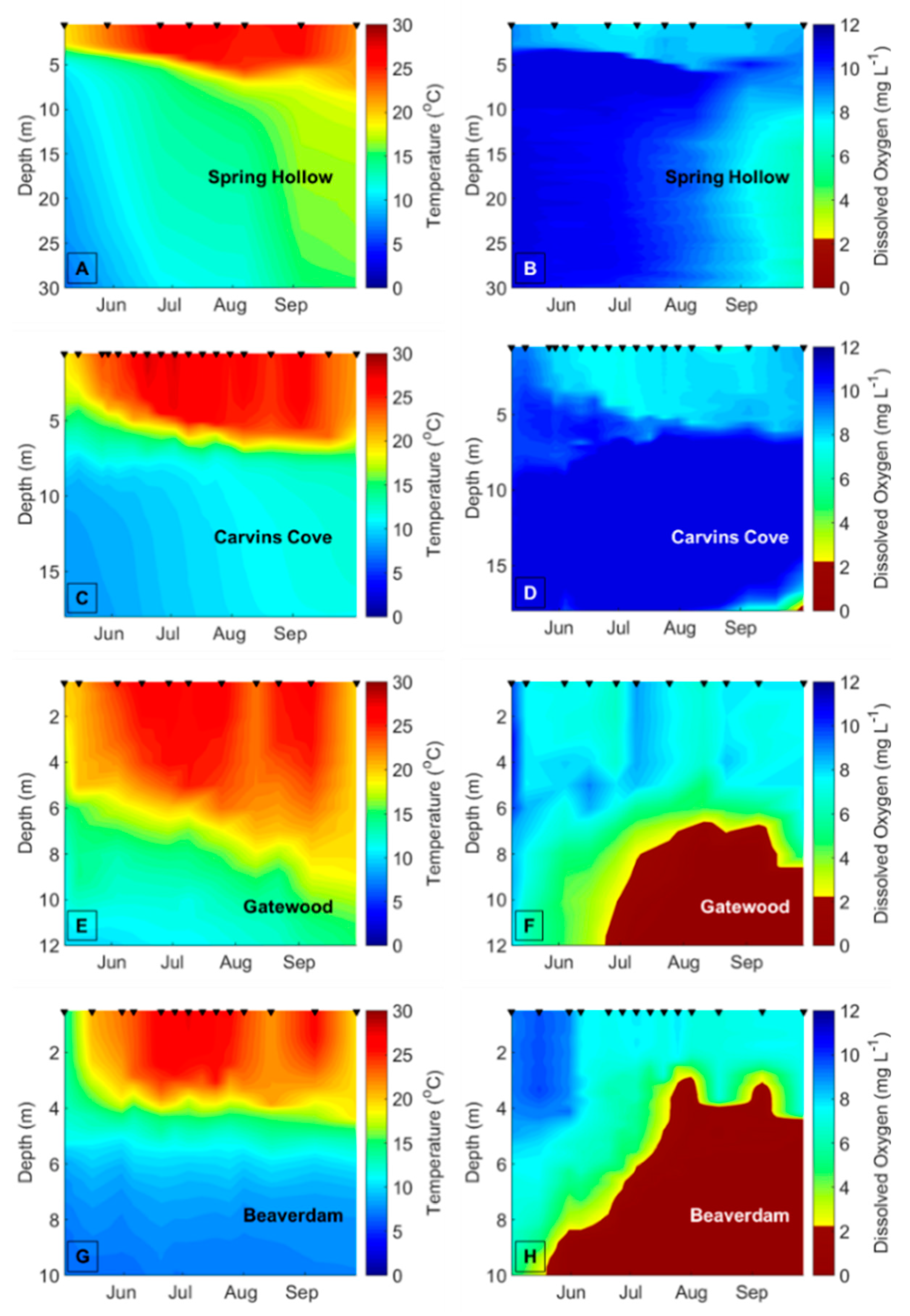
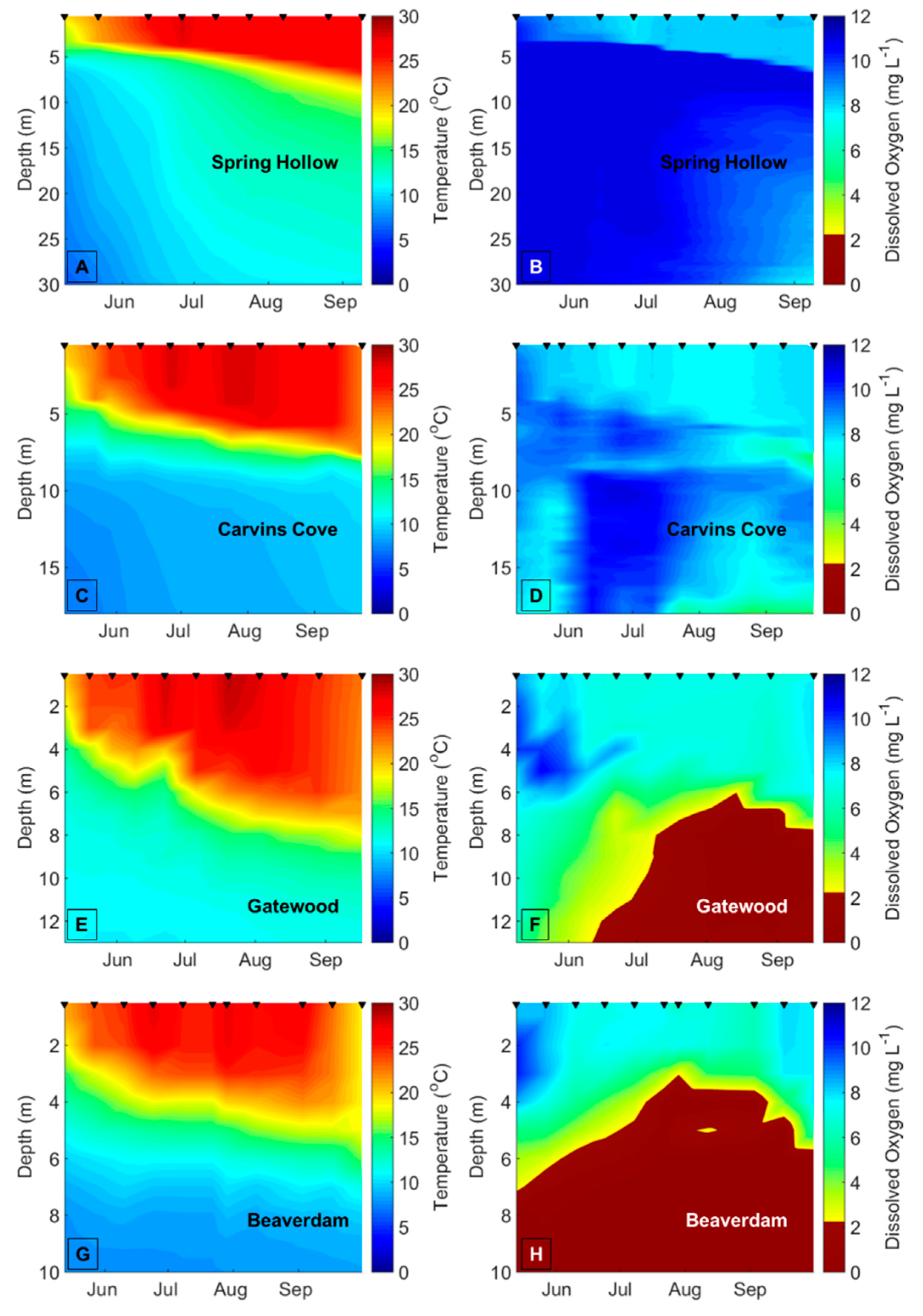
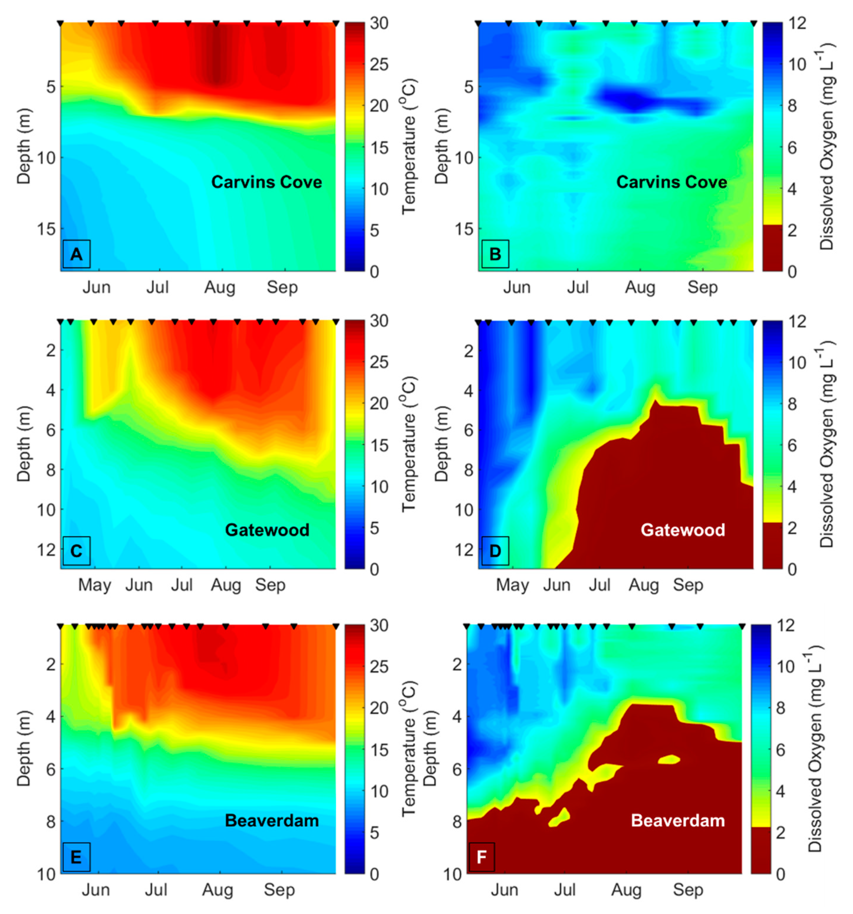
To demarcate the early vs. late stratified periods each year in BVR and GWR, the two reservoirs that exhibited summer hypolimnetic hypoxia, we first determined the depth of the thermocline on each sampling date using rLakeAnalyzer [54], and then calculated the mean hypolimnetic DO concentrations on the sampling dates from the CTD or YSI DO profiles. We used the mean hypolimnetic DO concentrations to identify the timing of the oxic (DO > 2 mg L−1) and hypoxic (DO ≤ 2 mg L−1) periods within each summer (Table A1). The hypolimnion in GWR and BVR became hypoxic between late June and mid-July every year, except in BVR in 2015, when the hypolimnion became hypoxic prior to the beginning of the sampling season (14 May), so it was impossible to demarcate the onset of hypoxia in the BVR that year. We assigned 20 July as the breakpoint between the early and late stratified periods in CCR and SHR, the two reservoirs that never exhibited hypoxia, across all years because both BVR and GWR always exhibited hypolimnetic hypoxia after this date every year, and this delineation evenly divided the number of sampling dates between the early and late stratified periods. To ensure that our results were not confounded by the delineation of the early vs. late stratified periods, we reran all analyses with different breakpoints between the early and late stratified period that ranged from ± 1 week of the oxic/hypoxic boundaries (Table A2 and Table A3).
We then calculated the biomass variability of crustacean, copepod and cladoceran zooplankton measured on sample days within the early stratified vs. late stratified periods for each reservoir and year. To account for different numbers of sampling dates in the early vs. late stratified periods, we randomly sampled the minimum number of observations (n = 3) during the shortest early or late period 1000 times (mean n of observations within a period = 5.2 ± 2.1, 1 SD) [55,56]. We calculated the mean CV from the 1000 samples to ensure that the biomass variability estimates were comparable between early and late stratified periods. We similarly repeated the bootstrapping to calculate the compositional variability from the minimum number of observations during a stratified period. Only the compositional variability of the aggregated crustacean zooplankton community (not individual copepod or cladoceran groups) was calculated, since there were only two copepod genera in the reservoirs.
Wilcoxon signed rank tests were performed to compare changes in the biomass variability and compositional variability of the reservoirs’ zooplankton communities between the early and late stratified periods. We grouped the reservoirs by whether they exhibited summer hypolimnetic hypoxia (i.e., oxic CCR and SHR vs. hypoxic BVR and GWR) and performed the two-tailed tests separately for the biomass variability of total crustacean, copepod, and cladoceran zooplankton and the compositional variability of crustacean zooplankton biomass in the oxic vs. hypoxic reservoirs. Wilcoxon signed rank tests were required because there was not a seasonally oxic period of the sampling season for BVR in 2015, and no samples were analyzed from SHR in 2016, creating an unbalanced design.
Finally, we analyzed the differences in mean hypolimnetic DO concentration, water column temperature, mean epilimnetic phytoplankton biomass, Secchi disk depth, TN concentration and TP concentration between the early vs. late stratified periods with Wilcoxon signed rank tests. These analyses were performed to assess which environmental variables other than hypolimnetic DO concentrations changed between the periods.
All analyses were performed in R v.3.5.1 (R Core Development Team, 2018). Given the small number of reservoirs in our analyses, we interpreted statistical significance at α = 0.10.

4. Results

4.1. Seasonal Temperature, DO, Water Chemistry, and Phytoplankton Biomass

The four reservoirs exhibited similar thermal structure throughout the sampling period. Thermal stratification developed at the beginning of May in all four reservoirs in all three years (Figure 1A,C,E,G; Figure A1 and Figure A2), which exhibited similar mean seasonal thermocline depths across all three years (CCR: 6.6 ± 1.0 m (1 SD), SHR: 5.0 ± 0.8 m, BVR: 4.4 ± 0.9 m, GWR: 6.6 ± 1.7 m). The water temperatures of the four reservoirs were similar, with maximum epilimnetic temperatures of 27–30 °C and hypolimnetic temperatures between 10–15 °C during the monitoring period across years. Both oxic and hypoxic reservoirs exhibited warming water column maximum temperatures between the early and late stratified periods, with a slightly greater mean increase in the hypoxic reservoirs than the oxic reservoirs (2.62 ± 1.65 °C vs. 1.78 ± 1.32 °C, respectively; Table 2; Figure 2C,D).
Although thermal structure was relatively similar across the reservoirs and across the years, DO concentrations were different. The hypolimnia of the CCR and SHR remained oxic throughout the monitoring period in May–September every year (Figure 1B,D; Figure A1 and Figure A2). In contrast, the hypolimnia of both GWR (Figure 1F) and the BVR (Figure 1H) were oxic at the onset of thermal stratification but became hypoxic generally in late-June to mid-July in the GWR and mid-June to early-July in the BVR, except for in 2015. In 2015, the hypolimnion of the BVR became hypoxic at the onset of thermal stratification at the beginning of the sampling season in mid-May (Table A1; Figure A1). Mean hypolimnetic DO concentration was approximately 7× lower in the late stratified period in BVR and GWR vs. in those two reservoirs’ early stratified periods (early vs. late mean hypolimnetic DO concentration: 4.6 ± 0.8 mg L−1 vs. 0.7 ± 0.3 mg L−1, respectively; Figure 2A,B). Wilcoxon signed rank tests confirm significant differences between the early vs. late stratified periods in the hypoxic, but not oxic, reservoirs (Table 2).
In addition to DO, other environmental variables exhibited differences between the early vs. late stratified periods among the reservoirs. Secchi disk depths were deeper in the SHR (8.8 ± 2.5 m, 1 SD) and CCR (4.2 ± 0.8 m) compared to GWR (3.5 ± 0.6 m) and BVR (3.1 ± 0.7 m) across years (Table 3). Nutrient concentrations and phytoplankton biomass were generally lower in the SHR and CCR compared to the GWR and BVR across years (Table 3). Generally, water quality improved in the oxic reservoirs in the late vs. early stratified period (as indicated by significantly deeper Secchi disk depths and lower TP concentrations), while water quality decreased in the hypoxic reservoirs (as indicated by significantly greater phytoplankton biomass and TN concentrations; Figure 2E,F; Table 2; Table 3).

4.2. Zooplankton Seasonal Biomass Dynamics

Seasonal crustacean zooplankton biomass varied substantially among the reservoirs (Figure 3). Mean crustacean zooplankton biomass in SHR (43.3 ± 33.7 µg DW L−1, 1 SD) was more than 2× greater than in CCR (17.7 ± 9.6 µg DW L−1) and GWR (18.6 ± 14.7 µg DW L−1), and 6× greater than in BVR (6.9 ± 5.3 µg DW L−1) across years and the stratified period.
CCR, SHR and BVR generally exhibited their crustacean zooplankton biomass maximum in June or July, as is expected from typical seasonal succession. A zooplankton peak was not discernable in BVR in 2015, when the hypolimnion of BVR became hypoxic early in the stratified period (Figure 3C). GWR did not have a crustacean zooplankton biomass maximum in June or July; however, it is possible that the zooplankton peak in this GWR occurred before our sampling period started (Figure 3D) because crustacean zooplankton biomass was often relatively high on the first sampling date in May. The crustacean zooplankton biomass in BVR varied substantially within the late stratified period and across years, with no consistent patterns (Figure 3C).
The zooplankton community in the late stratified period of the seasonally hypoxic reservoirs varied substantially from the zooplankton community in the late stratified period in the seasonally oxic reservoirs (Table 4; Figure 4; Figure A3). SHR was the only reservoir that was dominated by Daphnia spp., mainly Daphnia catawba (Figure 4B). Daphnia spp. comprised 63.5 ± 27.2% of the crustacean zooplankton biomass across years in SHR (82.6 ± 9.7% in the early stratified period and 39.6 ± 22.3% in the late stratified period), whereas Daphnia spp. only comprised 8.5 ± 17.5% of the crustacean zooplankton community across all years in CCR, BVR and GWR (Figure 4A,C,D; Table 4; Figure A3).
In contrast to SHR, the crustacean zooplankton communities in CCR, BVR, and GWR were largely dominated by cyclopoid copepods, mainly Mesocyclops spp., regardless of the stratified period. Cyclopoids comprised 66.8 ± 22.6% of the crustacean zooplankton biomass across years in CCR, BVR, and GWR (range: 55.2–77.5%), and only comprised 22.5 ± 15.2% across years in SHR (Figure 4; Table 4; Figure A3). The copepod Diaptomus sicilis comprised 23.3 ± 18.2% and 13.6 ± 14.3% of the crustacean zooplankton biomass across years in CCR and SHR, respectively, but less than 3% of the crustacean zooplankton biomass in BVR and GWR (Figure 4). D. sicilis had greater dominance in the zooplankton community in the late stratified period in CCR (37.5 ± 14.1%) and SHR (25.2 ± 14.5%) vs. the late stratified period in the hypoxic reservoirs. Other zooplankton taxa (e.g., Bosmina longirostris, Ceriodaphnia spp. Chydorus spp., and Diaphanosoma spp.) generally comprised < 5–10% of the zooplankton biomass when present, and these smaller cladoceran taxa were generally more dominant in the late stratified period in the seasonally hypoxic reservoirs vs. the seasonally oxic reservoirs (Figure 4C,D).

4.3. Biomass Variability of Zooplankton Communities

No significant effect of year existed for crustacean zooplankton, cladoceran and copepod biomass variability (Kruskal-Wallis: All H ≤ 2.96, P ≥ 0.23). Therefore, we treated each year as an independent replicate for subsequent analyses.
No significant difference existed in total crustacean and cladoceran zooplankton biomass variability in the oxic reservoirs between the early and late stratified periods (Wilcoxon signed rank tests: P ≥ 0.13; Table 5, Figure 5C). However, contrary to our prediction, the seasonally hypoxic reservoirs had significantly higher total crustacean, cladoceran and copepod biomass variability in the late stratified period than in the early stratified period (P ≤ 0.06; Table 5, Figure 5B,D). Total crustacean zooplankton and copepod biomass variability was ~2× greater later in the season when hypolimnetic hypoxia developed in the seasonally hypoxic reservoirs compared to the early stratified period when those reservoirs’ hypolimnia were still oxic. The copepod community exhibited a significant decrease in biomass variability from the early to late stratified period in the oxic reservoirs, opposite from the increase in the hypoxic reservoirs (Figure 5A; Table 5). The overall results were similar regardless of which early vs. late stratified period breakpoint was used (Table A2 and Table A3); crustacean zooplankton and copepod biomass variability remained significantly higher in the late vs. early stratified period in the seasonally hypoxic reservoirs, but not in the oxic reservoirs. Cladoceran biomass variability was significantly higher in the late vs. early stratified period in the seasonally hypoxic reservoirs when the season breakpoint was one week earlier, but not one week later (Table A2 and Table A3).

4.4. Compositional Variability of Zooplankton Communities

Just as with biomass variability, there was no significant effect of year on compositional crustacean zooplankton variability (Kruskal-Wallis: H ≤ 0.21; P ≥ 0.90). Therefore, we treated each year as an independent replicate for analysis on the effects of hypolimnetic hypoxia on the compositional variability of crustacean zooplankton biomass.
Counter to our original predictions and similar to biomass variability, the seasonally hypoxic reservoirs (BVR and GWR) had a significantly greater compositional variability of crustacean zooplankton in the late stratified period than the early stratified period, while compositional variability did not significantly change in the oxic reservoirs (CCR and SHR) between the late and early stratified periods (Table 5; Figure 6A,B). In the late stratified period, the compositional variability was 1.5 to 2× greater in reservoirs with hypoxic hypolimnia versus the reservoirs with oxic hypolimnia. Results were similar regardless of the breakpoint date between early and late stratified periods (Table A2 and Table A3), except that seasonally oxic reservoirs had a significantly lower crustacean zooplankton compositional variability in the late vs. early stratified period when the season breakpoint demarcation was one week later (Table A2).

5. Discussion

Global change is predicted to create more variable environmental conditions [1,2,3], which can alter community interactions and the variability of ecological communities [4,5,6]. Contrary to our predictions, we found that hypolimnetic hypoxia was associated with an increased biomass variability and compositional variability of crustacean zooplankton communities in reservoirs. Our data suggest that the variability of zooplankton communities may increase with hypolimnetic hypoxia in temperate inland waterbodies.
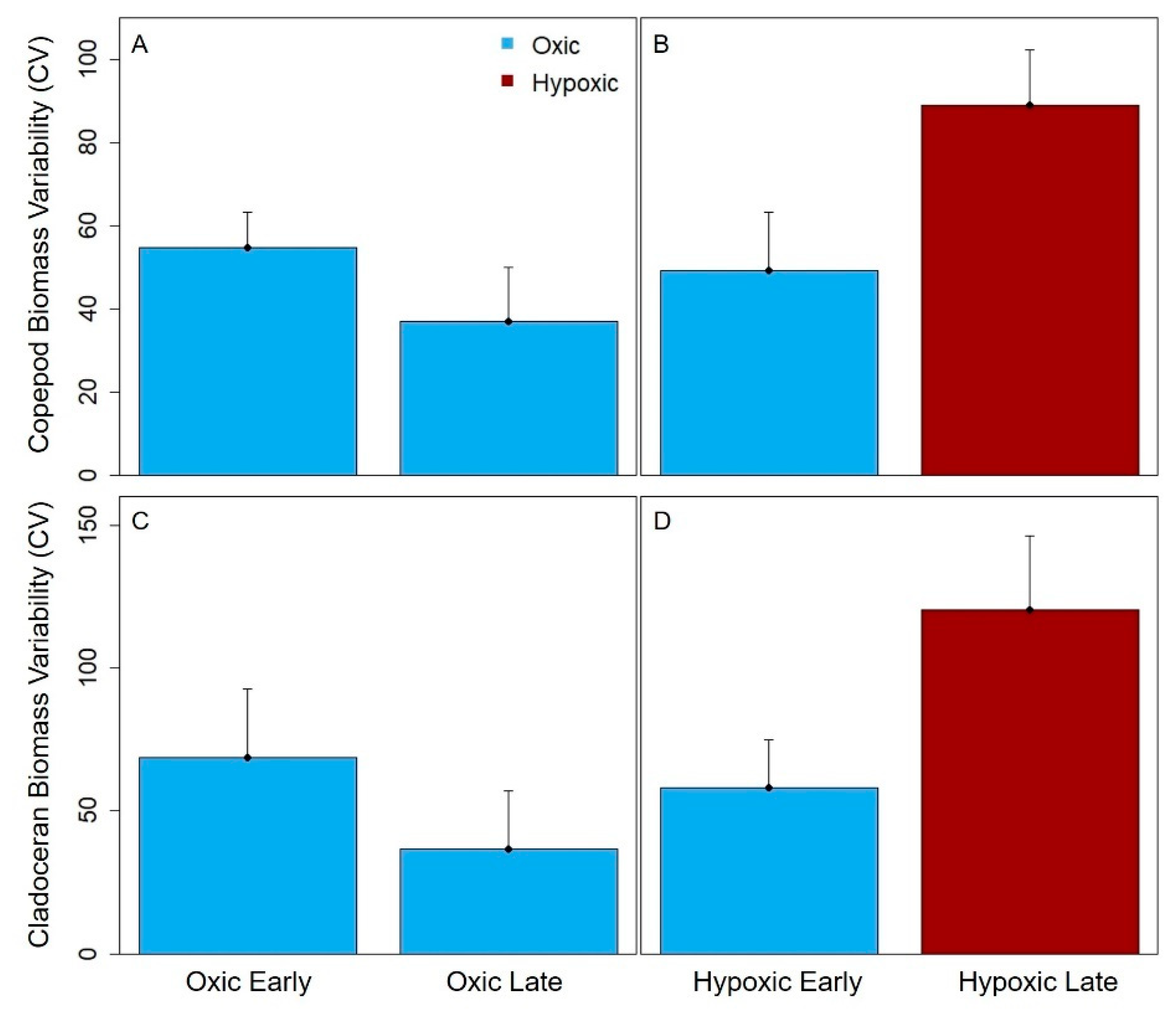
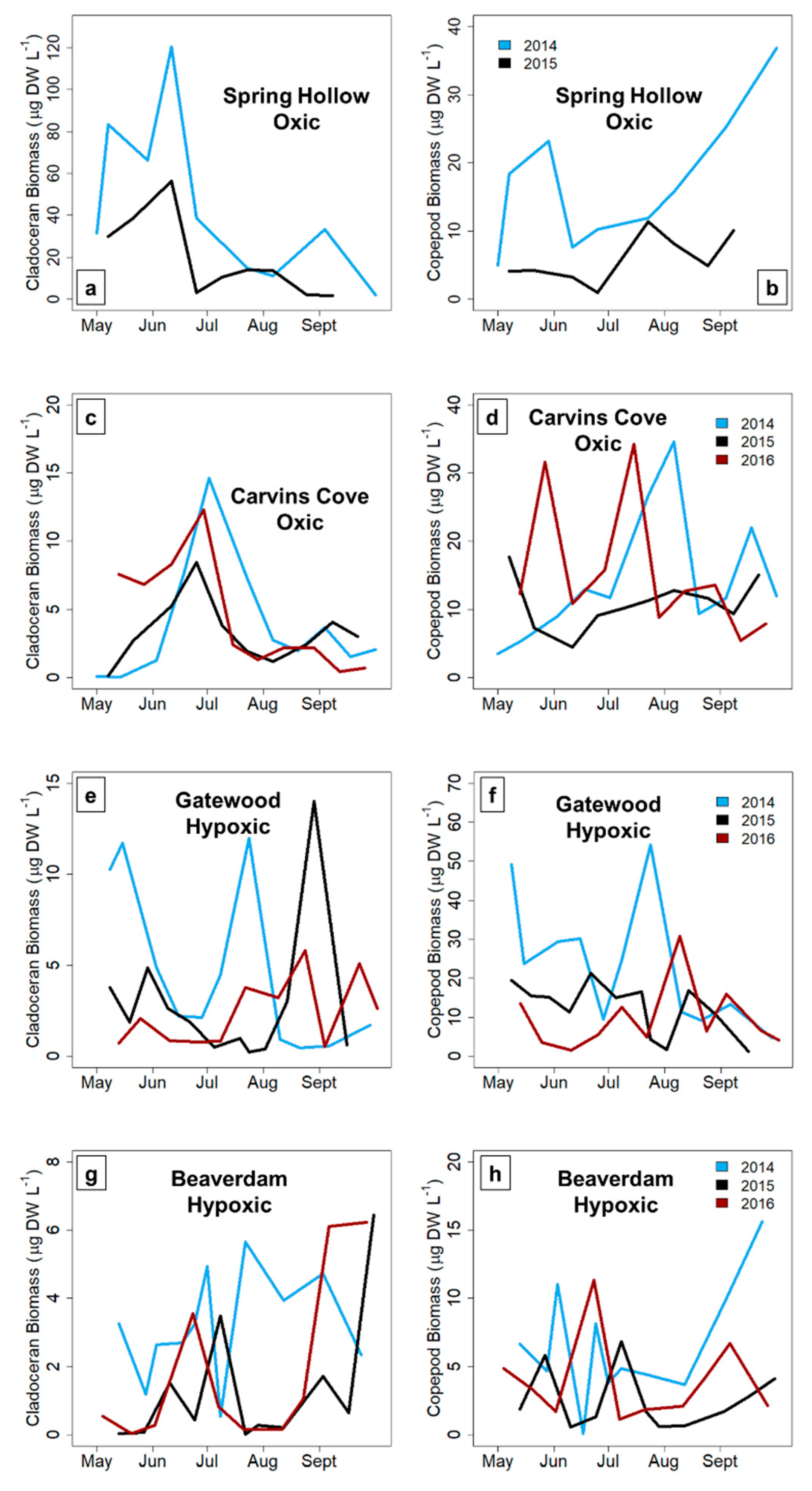
Total crustacean, cladoceran and copepod zooplankton biomass variability significantly increased from the early to late stratified period in the hypoxic reservoirs, but did not significantly change in the seasonally oxic reservoirs in the late stratified period (except for the copepods, which exhibited a decrease in biomass variability). The biomass variability increase in the hypoxic reservoirs was largely driven by copepods, which are generally the dominant group of zooplankton present in temperate waterbodies in the late stratified period [26,
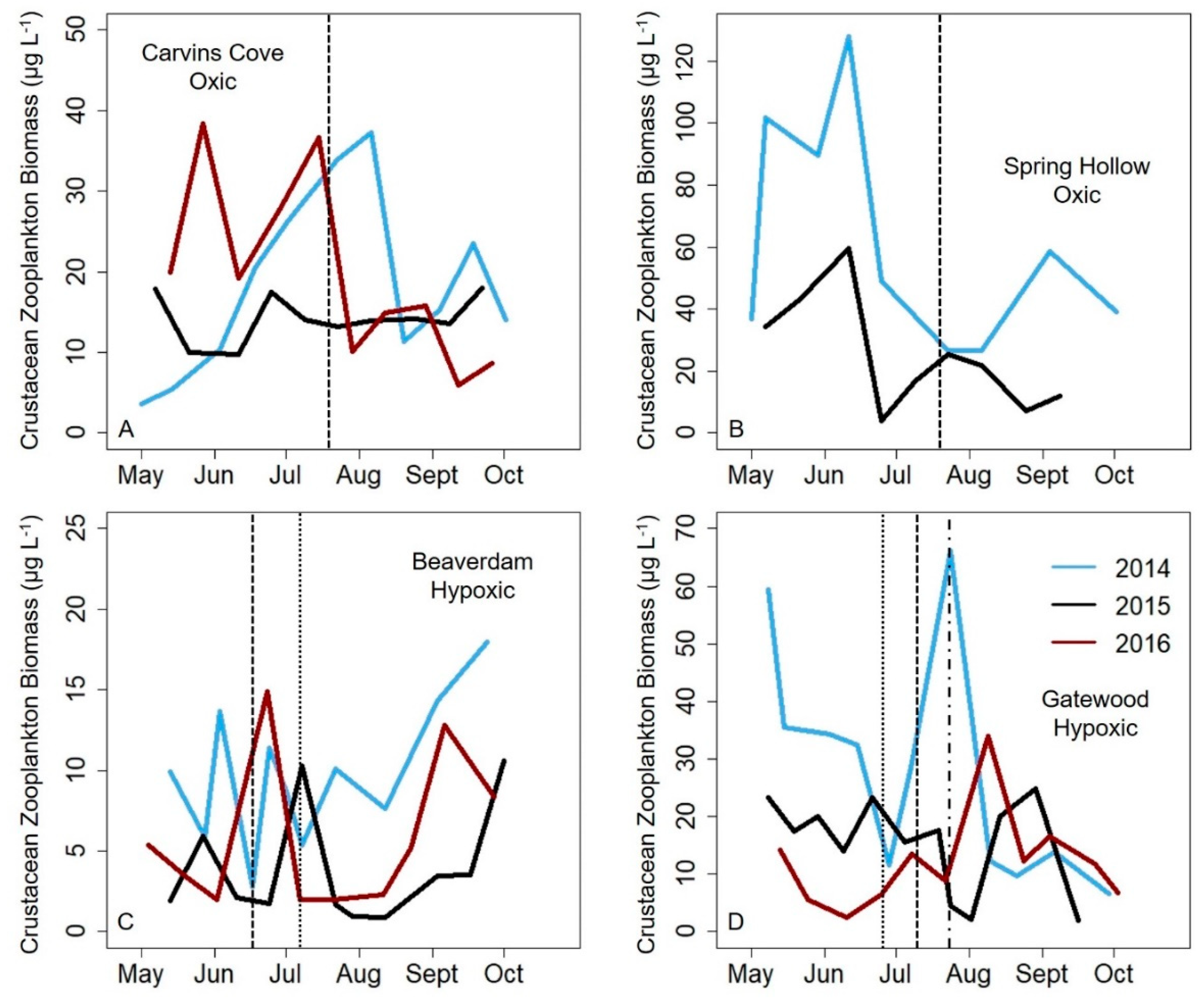
27]. In almost all reservoirs and years, a zooplankton maximum was present in the early stratified period in each reservoir (except the GWR, but it is possible that we missed the spring zooplankton maximum because the first sampling date during the three study years often exhibited higher biomass). In contrast, although a second, smaller zooplankton biomass maximum occurred in the late stratified period in the oxic CCR and SHR, this peak did not consistently occur in the hypoxic BVR and GWR reservoirs, driving the biomass variability difference. The magnitude of the biomass maximum in the BVR and GWR in the late stratified season varied by ~9× in both reservoirs among years, in comparison to an ~3× and ~2× difference in biomass among years for CCR and SHR, respectively. Therefore, our data suggest that hypolimnetic hypoxia may increase the biomass variability of zooplankton communities, resulting in a larger deviation from the typical pattern of zooplankton seasonal succession that occurs in the late stratified period in more oxic systems.
One possible mechanism for increased biomass variability under hypoxic conditions is due to diel vertical migration (DVM) of crustacean zooplankton. DVM is a ubiquitous zooplankton behavior, in which a majority of the population migrates to the dark hypolimnion during the day to escape predation from fish and damaging ultraviolet (UV) radiation [33,34,57]. At nighttime, a large portion of the zooplankton population migrates back to the epilimnion, where they are closer to phytoplankton as a food resource, with a decreased risk of being eaten, or ending up damaged by UV radiation. However, because zooplankton also need oxygen for respiration [20,21], they may be forced out of the safety of the hypolimnion during the daytime and instead remain in the epilimnion, trading oxic stress for increased risk of predation or UV radiation damage [35]. Subsequently, the increase in the biomass variability of the zooplankton community during hypolimnetic hypoxic periods may be related to sporadic pulses of zooplankton taxa that suddenly increase due to emergence from sediment resting stages, and then shortly thereafter exhibit population crashes due to fish predation in the epilimnion or the deleterious effects of UV radiation. Additional data are needed to support these hypotheses, which were not possible to examine within our study scope.
In the hypoxic BVR and GWR, cyclopoid copepods primarily drove the pattern of increased biomass variability in the late stratified period. Because copepods have longer generation times than cladocera and are generally conspicuous for fish in well-lit waters due to their more opaque coloration, copepods are more likely to conduct DVM, and hence may be sensitive to hypolimnetic hypoxia [28,58], resulting in greater variability in their biomass during hypoxic conditions. In contrast, late season copepods in the oxic reservoirs did not exhibit as many fluctuations in their biomass, resulting in a decrease in their biomass variability throughout the stratified period (Figure 5A). While cladocera are expected to be less sensitive to hypoxia than copepods because they are more transparent and overall much smaller [26,59], thereby allowing them some release from visual predators (i.e., fish), we observed that the biomass variability of both taxa increased with the onset of hypoxia. Thus, our results suggest that hypoxia may affect the entire crustacean zooplankton community, though future studies are needed to directly assess the effects of hypoxia on individual zooplankton at a finer taxonomic level.
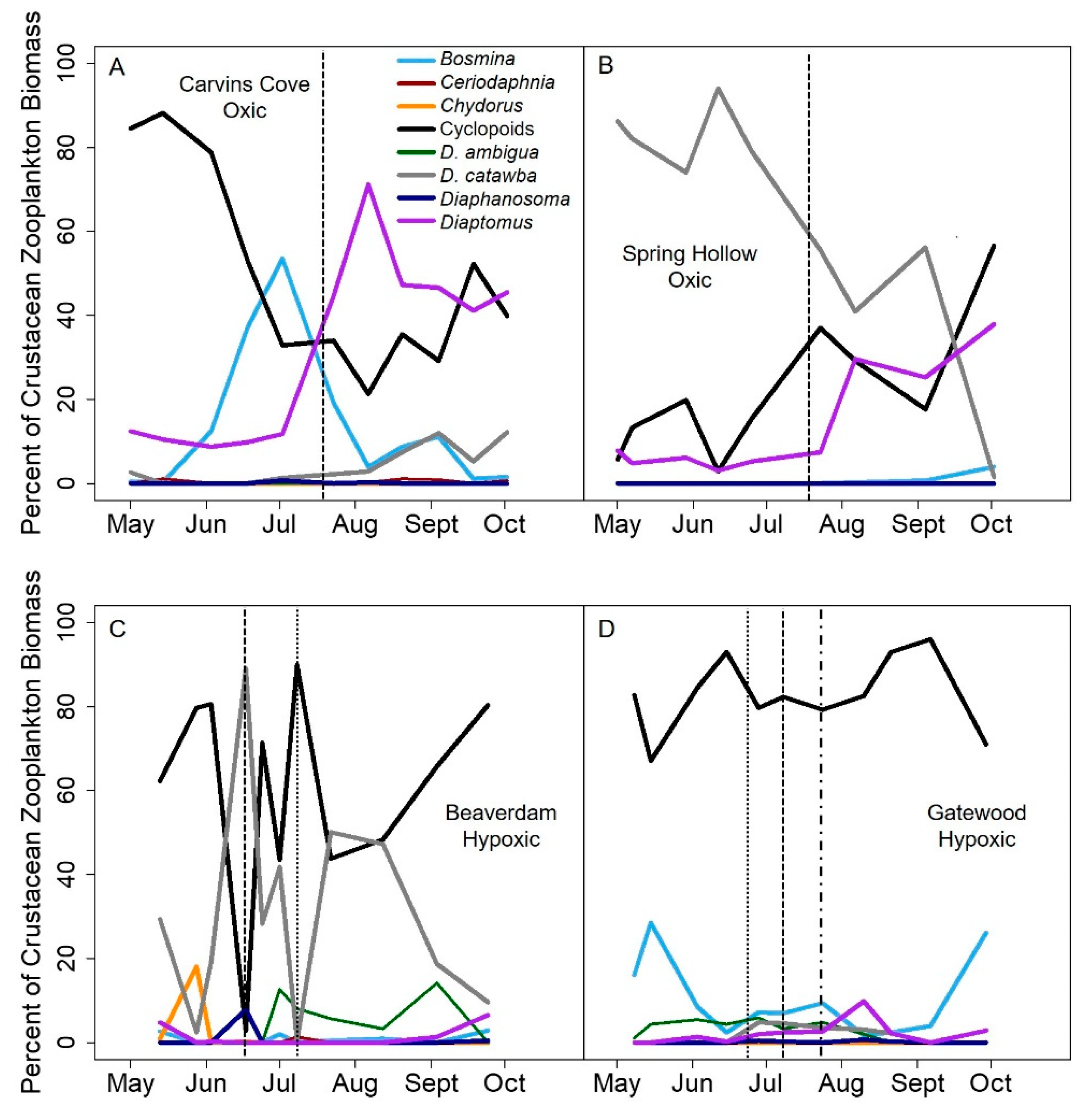
Counter to our predictions, we found that hypolimnetic hypoxia also increased the compositional variability for the dominance in crustacean zooplankton communities. The seasonally hypoxic reservoirs were more likely to be dominated by one or just a few taxa, primarily cyclopoid copepods and smaller cladocera, than the oxic reservoirs in the late stratified period (Figure 4). Following the hypothesis above, possibly the substantial day-to-day variability in the biomass of those dominant taxa drove the greater compositional variability in the hypoxic reservoirs than oxic reservoirs in the late stratified period. However, we were not able to test the specific mechanisms underlying the compositional variability differences between hypoxic and oxic reservoirs.
Hypolimnetic hypoxia was likely the main driver of the observed changes in the biomass variability and compositional variability of the crustacean zooplankton community. The mean hypolimnetic DO concentration decreased by about 7× in the late vs. early stratified period in the seasonally hypoxic reservoirs. In contrast, the mean hypolimnetic DO changed only slightly in the early vs. late stratified periods of the seasonally oxic reservoirs, which is likely why there were fewer differences in the variability of the zooplankton communities in these reservoirs. Changes in the other environmental variables between the early and late stratified periods are likely related to DO concentrations. For example, the significant increases in TN concentrations and phytoplankton biomass between the early and late stratified periods in the BVR and GWR may be related to the release of nutrients from the sediments to the water column that occurs under hypoxic conditions [60,61,62] and the subsequent stimulation of primary productivity.
Because crustacean zooplankton feed on phytoplankton [24,42,63], increased phytoplankton biomass in the hypoxic reservoirs throughout the summer may have also amplified the biomass variability and compositional zooplankton variability differences between reservoirs. An increase in the Secchi disk depth and decrease in TP concentrations also existed in the seasonally oxic reservoirs from the early to late stratified period (but not in the hypoxic reservoirs), which may have also played a factor in the variability differences. Altogether, our data support [64]’s paradox of enrichment, in that greater food availability (phytoplankton biomass) results in greater variability of the predator (zooplankton) populations. While we are unable to model phytoplankton –zooplankton populations given the coarse temporal resolution of our sampling relative to phytoplankton generation times, our study adds field survey data to previous microcosm [65] and paleolimnological [12] studies that observed similar variability patterns.
A limitation of our work was that we were unable to account for some other environmental factors that may also affect the variability in zooplankton communities. For example, there may have been differences in fish grazing rates [66,67], disease transmission [68], diel horizontal migration [69,70], or interactions among multiple variables that may have also affected zooplankton community variability. Also, the demarcation of the early vs. late stratified period inherently created non-independence between zooplankton samples and the other environmental variables across the season that we were not able to fully account for. Finally, the patterns of biomass variability and compositional variability were dependent upon the taxa present in our study systems; the results might be different in other lakes and reservoirs with different zooplankton assemblages.
Our work suggests that increases in hypolimnetic hypoxia intensity and duration may alter the biomass variability and compositional variability of zooplankton, thereby altering the seasonal succession dynamics of the zooplankton communities. The alteration of zooplankton communities could also lead to changes in the populations in other trophic levels (phytoplankton and fish), which has implications for water quality. Therefore, it is critically important to better understand the variability of ecological communities in waterbodies, and what the resulting consequences may be for ecosystem functioning and processes.

Author Contributions

J.P.D. and C.C.C. conceived the project idea. All authors collected field data. J.P.D. and K.L.C. counted zooplankton samples. J.P.D., K.L.C., C.C.C., M.E.L., and R.P.M. analyzed data. J.P.D. and C.C.C. wrote the manuscript and all authors provided feedback and approved the final manuscript version.

Funding

The research was funded by the National Science Foundation DEB-1601061, ICER-1517823, ER-1702506, CNS-1737424, and DEB-1753639.

Acknowledgments

We thank the National Science Foundation DEB-1601061, ICER-1517823, ER-1702506, CNS-1737424, DEB-1753639, the Global Lake Ecological Observatory Network, Virginia Tech Fralin Life Sciences Institute, Virginia Tech Global Change Center, Virginia Tech Institute for Critical Technology and Applied Science, and Virginia Water Resources Research Center for financial support for this research. We are grateful to the Western Virginia Water Authority and the Pulaski Parks and Facilities Department for sampling access to the reservoirs. We thank B. L. Brown and K. J. Farrell for statistical consulting and graphing advice, S. K. Goldfarb for helpful comments on the manuscript, and A. B. Gerling, K. D. Hamre, C. W. Harrell, D. W. Howard, Z. W. Munger, M. F. Ryan, N. K. Ward, and B. Thompson for help in field sampling and laboratory analyses.

Conflicts of Interest

The authors declare no conflict of interest.

Appendix A

Table A1. Dates of hypolimnetic hypoxia onset (mean hypolimnetic dissolved oxygen concentrations ≤2 mg L−1) in the two seasonally hypoxic reservoirs, Beaverdam and Gatewood. 14 May was the first sampling day for Beaverdam in 2015.
ReservoirYearDate of Hypolimnetic Hypoxia
Beaverdam201418 June
Beaverdam2015Before 14 May
Beaverdam20167 July
Gatewood20149 July
Gatewood201520 July
Gatewood201625 June
Table A2. Wilcoxon signed rank test statistics of the difference in crustacean zooplankton, cladoceran and copepod biomass variability and the compositional variability of crustacean zooplankton biomass between the early (when all reservoirs were oxic) and late stratified periods across years in oxic and hypoxic reservoirs, when the breakpoint between the early and late stratified period was 1 week later than shown in Table 5. Only the compositional variability of total crustacean zooplankton (not individual copepod or cladocera group taxa) was calculated, because there were only two copepod taxa present in the reservoirs. A positive mean difference tells us that the value increased from the early to late stratified period. Bold P-values highlight statistically significant (P < 0.10) two-tailed P-values.
Response VariableTaxonHypolimnetic Oxygen RegimeMean Difference between Early and Late Stratified PeriodWilcoxon Signed Rank Test StatisticP-Value
Biomass variabilityCrustaceansOxic−12.97−6.500.13
Hypoxic48.317.500.06
CopepodsOxic1.75−0.501.00
Hypoxic37.297.500.06
CladoceraOxic−14.07−4.500.31
Hypoxic37.676.500.13
Compositional variability CrustaceansOxic−0.08−7.500.06
Hypoxic0.117.500.06
Table A3. Wilcoxon signed rank test statistics of the difference in crustacean zooplankton, cladoceran and copepod biomass variability, and the compositional variability of crustacean zooplankton biomass between the early (when all reservoirs were oxic) and late stratified periods across years in oxic and hypoxic reservoirs, when the breakpoint between early and late stratified period was 1 week earlier than shown in Table 5. Only the compositional variability of total crustacean zooplankton (not individual copepod or cladoceran group taxa) was calculated, because there were only two copepod taxa present in the reservoirs. A positive mean difference shows that the value increased from the early to late stratified period. Bold P-values highlight statistically significant (P < 0.10) two-tailed P-values.
Response VariableTaxonHypolimnetic Oxygen RegimeMean Difference between Early and Late Stratified PeriodWilcoxon Signed Rank Test StatisticP-Value
Biomass variabilityCrustaceansOxic−12.28−5.500.19
Hypoxic45.017.500.06
CopepodsOxic−29.91−3.500.44
Hypoxic39.727.500.06
CladoceraOxic−10.00−5.500.19
Hypoxic62.357.500.06
Compositional variability (Bray-Curtis)CrustaceansOxic0.008−0.501.00
Hypoxic0.117.500.06
Figure A1. Temperature and dissolved oxygen depth profiles of the four focal reservoirs during the summer stratified period in 2015. The color scale for the dissolved oxygen concentrations highlights the hypoxia threshold at 2 mg L−1. The hypolimnia of Spring Hollow (A,B) and Carvins Cove (C,D) remained oxic; however, the hypolimnia of Gatewood (E,F) and Beaverdam (G,H) developed hypoxia. Black triangles on the top of each panel represent days sampled, and the intervening data were interpolated.
Water 11 02179 g0a1
Figure A2. Temperature and dissolved oxygen depth profiles of the focal reservoirs during the summer stratified period in 2016. The color scale for the dissolved oxygen concentrations highlights the hypoxia threshold at 2 mg L−1. The hypolimnia of Carvins Cove (A,B) remained oxic; however, the hypolimnia of Gatewood (C,D) and Beaverdam (E,F) developed hypoxia. Black triangles on the top of each panel represent days sampled, and the intervening data were interpolated.
Water 11 02179 g0a2
Figure A3. Seasonal and inter-annual cladoceran and copepod biomass dynamics in the two seasonally oxic reservoirs (Spring Hollow: A,B; Carvins Cove: C,D) and the two seasonally hypoxic reservoirs (Gatewood: E,F; Beaverdam: G,H). Note the differences in the range of biomass between the reservoirs.
Water 11 02179 g0a3

References

  1. Easterling, D.R. Climate Extremes: Observations, Modeling, and Impacts. Science 2000, 289, 2068–2074. [Google Scholar] [CrossRef] [PubMed] [Green Version]
  2. Diffenbaugh, N.S.; Pal, J.S.; Trapp, R.J.; Giorgi, F. Fine-scale processes regulate the response of extreme events to global climate change. Proc. Natl. Acad. Sci. USA 2005, 102, 15774–15778. [Google Scholar] [CrossRef] [PubMed] [Green Version]
  3. Xenopoulos, M.A.; Lodge, D.M.; Alcamo, J.; Marker, M.; Schulze, K.; Van Vuuren, D.P.; Maerker, M. Scenarios of freshwater fish extinctions from climate change and water withdrawal. Glob. Chang. Boil. 2005, 11, 1557–1564. [Google Scholar] [CrossRef]
  4. Walther, G.-R.; Post, E.; Convey, P.; Menzel, A.; Parmesan, C.; Beebee, T.J.C.; Fromentin, J.-M.; Hoegh-Guldberg, O.; Bairlein, F. Ecological responses to recent climate change. Nature 2002, 416, 389–395. [Google Scholar] [CrossRef]
  5. Tylianakis, J.M.; Didham, R.K.; Bascompte, J.; Wardle, D.A. Global change and species interactions in terrestrial ecosystems. Ecol. Lett. 2008, 11, 1351–1363. [Google Scholar] [CrossRef]
  6. Eloire, D.; Somerfield, P.J.; Conway, D.V.P.; Halsband-Lenk, C.; Harris, R.; Bonnet, D. Temporal variability and community composition of zooplankton at station L4 in the Western Channel: 20 years of sampling. J. Plankton Res. 2010, 32, 657–679. [Google Scholar] [CrossRef] [Green Version]
  7. Cottingham, K.L.; Bascompte, J.; Eckert, G.L.; Fischer, J.M.; Keitt, T.H.; Kendall, B.E.; Rusak, J.A.; Micheli, F.; Bjørnstad, O.N.; Rusak, J.L.K.A. The Dual Nature of Community Variability. Oikos 1999, 85, 161. [Google Scholar] [Green Version]
  8. Brown, B.; Lennon, J.; Cottingham, K. Biodiversity may regulate the temporal variability of ecological systems. Ecol. Lett. 2001, 4, 72–85. [Google Scholar]
  9. Collins, S.; Micheli, F.; Hartt, L. A method to determine rates and patterns of variability in ecological communities. Oikos 2000, 91, 285–293. [Google Scholar] [CrossRef]
  10. Brown, B.L. Spatial heterogeneity reduces temporal variability in stream insect communities. Ecol. Lett. 2003, 6, 316–325. [Google Scholar] [CrossRef]
  11. Brown, B.L. Habitat heterogeneity and disturbance influence patterns of community temporal variability in a small temperate stream. Hydrobiologia 2007, 586, 93–106. [Google Scholar] [CrossRef]
  12. Cottingham, K.; Rusak, J.; Leavitt, P. Increased ecosystem variability and reduced predictability following fertilisation: Evidence from palaeolimnology. Ecol. Lett. 2000, 3, 340–348. [Google Scholar] [CrossRef]
  13. Kolar, C.S.; Rahel, F.J. Interaction of a biotic factor (predator presence) and an abiotic factor (low oxygen) as an influence on benthic invertebrate communities. Oecologia 1993, 95, 210–219. [Google Scholar] [CrossRef] [PubMed]
  14. Ludsin, S.A.; Zhang, X.; Brandt, S.B.; Roman, M.R.; Boicourt, W.C.; Mason, D.M.; Costantini, M. Hypoxia-avoidance by planktivorous fish in Chesapeake Bay: Implications for food web interactions and fish recruitment. J. Exp. Mar. Boil. Ecol. 2009, 381, S121–S131. [Google Scholar] [CrossRef]
  15. Winder, M.; Schindler, D.E. Climatic effects on the phenology of lake processes. Glob. Chang. Boil. 2004, 10, 1844–1856. [Google Scholar] [CrossRef] [Green Version]
  16. Jankowski, T.; Livingstone, D.M.; Bührer, H.; Forster, R.; Niederhauser, P. Consequences of the 2003 European heat wave for lake temperature profiles, thermal stability, and hypolimnetic oxygen depletion: Implications for a warmer world. Limnol. Oceanogr. 2006, 51, 815–819. [Google Scholar] [CrossRef] [Green Version]
  17. Butcher, J.B.; Nover, D.; Johnson, T.E.; Clark, C.M. Sensitivity of lake thermal and mixing dynamics to climate change. Clim. Chang. 2015, 129, 295–305. [Google Scholar] [CrossRef] [Green Version]
  18. Diaz, R.J.; Rosenberg, R. Spreading Dead Zones and Consequences for Marine Ecosystems. Science 2008, 321, 926–929. [Google Scholar] [CrossRef]
  19. Marcé, R.; Garcia, J.C.; Armengol, J.; Rodríguez-Arias, M.À. El Niño Southern Oscillation and climate trends impact reservoir water quality. Glob. Chang. Boil. 2010, 16, 2857–2865. [Google Scholar] [CrossRef]
  20. Jenny, J.-P.; Francus, P.; Normandeau, A.; Lapointe, F.; Perga, M.-E.; Ojala, A.; Schimmelmann, A.; Zolitschka, B.; Jenny, J.; Perga, M.; et al. Global spread of hypoxia in freshwater ecosystems during the last three centuries is caused by rising local human pressure. Glob. Chang. Boil. 2016, 22, 1481–1489. [Google Scholar] [CrossRef]
  21. Devol, A.H. Vertical distribution of zooplankton respiration in relation to the intense oxygen minimum zones in two British Columbia fjords. J. Plankton Res. 1981, 3, 593–602. [Google Scholar] [CrossRef]
  22. Stalder, L.C.; Marcus, N.H. Zooplankton responses to hypoxia: Behavioral patterns and survival of three species of calanoid copepods. Mar. Boil. 1997, 127, 599–607. [Google Scholar] [CrossRef]
  23. Roberts, J.J.; Höök, T.O.; Ludsin, S.A.; Pothoven, S.A.; Vanderploeg, H.A.; Brandt, S.B. Effects of hypolimnetic hypoxia on foraging and distributions of Lake Erie yellow perch. J. Exp. Mar. Boil. Ecol. 2009, 381, S132–S142. [Google Scholar] [CrossRef]
  24. Carpenter, S.R.; Kitchell, J.F.; Hodgson, J.R.; Cochran, P.A.; Elser, J.J.; Elser, M.M.; Lodge, D.M.; Kretchmer, D.; He, X.; Von Ende, C.N. Regulation of Lake Primary Productivity by Food Web Structure. Ecology 1987, 68, 1863–1876. [Google Scholar] [CrossRef] [Green Version]
  25. Threlkeld, S.T. Planktivory and planktivore biomass effects on zooplankton, phytoplankton, and the trophic cascade. Limnol. Oceanogr. 1988, 33, 1362–1375. [Google Scholar] [CrossRef]
  26. Sommer, U.; Gliwicz, M.; Lampert, W.; Duncan, A. The PEG-model of seasonal succession of planktonic events in fresh waters. Arch. Hydrobiol. 1986, 106, 433–471. [Google Scholar]
  27. Jürgens, K.; Stolpe, G. Seasonal dynamics of crustacean zooplankton, heterotrophic nanoflagellates and bacteria in a shallow, eutrophic lake. Freshw. Boil. 1995, 33, 27–38. [Google Scholar] [CrossRef]
  28. Vanderploeg, H.A.; Cavaletto, J.F.; Liebig, J.R.; Gardner, W.S. Limnocalanus macrurus (Copepoda: Calanoida) retains a marine arctic lipid and life cycle strategy in Lake Michigan. J. Plankton Res. 1998, 20, 2029. [Google Scholar] [CrossRef]
  29. Ekvall, M.K.; Hansson, L.-A. Differences in Recruitment and Life-History Strategy Alter Zooplankton Spring Dynamics Under Climate-Change Conditions. PLoS ONE 2012, 7, e44614. [Google Scholar] [CrossRef]
  30. Sorensen, M.L.; Branstrator, D.K. The North American invasive zooplanktivore Bythotrephes longimanus is less hypoxia-tolerant than the native Leptodora kindtii. Can. J. Fish. Aquat. Sci. 2017, 74, 824–832. [Google Scholar] [CrossRef] [Green Version]
  31. Kobayashi, M.; Hoshi, T. Relationship between the haemoglobin concentration of Daphnia magna and the ambient oxygen concentration. Comp. Biochem. Physiol. Part A Physiol. 1982, 72, 247–249. [Google Scholar] [CrossRef]
  32. Salonen, K.; Lehtovaara, A. Migrations of haemoglobin-rich Daphnia longispina in a small, steeply stratified, humic lake with an anoxic hypolimnion. Dissolved Org. Matter Lacustrine Ecosyst. Energy Source Syst. Regul. 1992, 229, 271–288. [Google Scholar]
  33. Zaret, T.M.; Suffern, J.S. Vertical migration in zooplankton as a predator avoidance mechanism. Limnol. Oceanogr. 1976, 21, 804–813. [Google Scholar] [CrossRef]
  34. Lampert, W. The Adaptive Significance of Diel Vertical Migration of Zooplankton. Funct. Ecol. 1989, 3, 21. [Google Scholar] [CrossRef]
  35. Doubek, J.P.; Campbell, K.L.; Doubek, K.M.; Hamre, K.D.; Lofton, M.E.; McClure, R.P.; Ward, N.K.; Carey, C.C. The effects of hypolimnetic anoxia on the diel vertical migration of freshwater crustacean zooplankton. Ecosphere 2018, 9, e02332. [Google Scholar] [CrossRef] [Green Version]
  36. Gantzer, P.A.; Bryant, L.D.; Little, J.C. Controlling soluble iron and manganese in a water-supply reservoir using hypolimnetic oxygenation. Water Res. 2009, 43, 1285–1294. [Google Scholar] [CrossRef]
  37. Bryant, L.D.; Hsu-Kim, H.; Gantzer, P.A.; Little, J.C. Solving the problem at the source: Controlling Mn release at the sediment-water interface via hypolimnetic oxygenation. Water Res. 2011, 45, 6381–6392. [Google Scholar] [CrossRef]
  38. Carey, C.C.; McClure, R.P.; Doubek, J.P.; Lofton, M.E.; Ward, N.K.; Scott, D.T. Chaoborus spp. Transport CH4 from the Sediments to the Surface Waters of a Eutrophic Reservoir, But Their Contribution to Water Column CH4 Concentrations and Diffusive Efflux Is Minor. Environ. Sci. Technol. 2018, 52, 1165–1173. [Google Scholar] [CrossRef]
  39. Gregor, J.; Maršálek, B. Freshwater phytoplankton quantification by chlorophyll a: A comparative study of in vitro, in vivo and in situ methods. Water Res. 2004, 38, 517–522. [Google Scholar] [CrossRef]
  40. Catherine, A.; Escoffier, N.; Belhocine, A.; Nasri, A.; Hamlaoui, S.; Yéprémian, C.; Bernard, C.; Troussellier, M. On the use of the FluoroProbe®, a phytoplankton quantification method based on fluorescence excitation spectra for large-scale surveys of lakes and reservoirs. Water Res. 2012, 46, 1771–1784. [Google Scholar] [CrossRef]
  41. Pannard, A.; Planas, D.; Beisner, B.E. Macrozooplankton and the persistence of the deep chlorophyll maximum in a stratified lake. Freshw. Boil. 2015, 60, 1717–1733. [Google Scholar] [CrossRef]
  42. Downing, J.A.; Rigler, F.H. Manual on Methods for the Assessment of Secondary Productivity in Fresh Waters; Blackwell Scientific Publications: Oxford, UK, 1984. [Google Scholar]
  43. Méthot, G.; Richard, N.; Pinel-Alloul, B.; Masson, S. Comparison of nets and pump sampling gears to assess zooplankton vertical distribution in stratified lakes. J. Plankton Res. 2004, 26, 1199–1206. [Google Scholar]
  44. Wetzel, R.G.; Likens, G.E. Limnological Analyses, 2nd ed.; Springer: New York, NY, USA, 1991. [Google Scholar]
  45. Lampert, W.; Fleckner, W.; Rai, H.; Taylor, B.E. Phytoplankon control by grazing zooplankton: A study on the spring clear-water phase. Limnol. Oceanogr. 1986, 31, 478–490. [Google Scholar] [CrossRef]
  46. Straile, D. Zooplankton biomass dynamics in oligotrophic versus eutrophic conditions: A test of the PEG model. Freshwater Biol. 2015, 60, 174–183. [Google Scholar] [CrossRef]
  47. Gerten, D.; Adrian, R. Climate-driven changes in the spring plankton dynamics and the sensitivity of shallow polymictic lakes to the North Atlantic Oscillation. Limnol. Oceanogr. 2000, 45, 1058–1066. [Google Scholar] [CrossRef]
  48. Brown, B.L.; Lawson, R.L. Habitat heterogeneity and activity of an omnivorous ecosystem engineer control stream community dynamics. Ecology 2010, 91, 1799–1810. [Google Scholar] [CrossRef] [Green Version]
  49. He, X.; Scheurell, M.D.; Soranno, P.A.; Wright, R.A. Recurrent response patterns of a zooplankton community to whole-lake fish manipulation. Freshw. Boil. 1994, 32, 61–72. [Google Scholar] [CrossRef]
  50. Yan, N.D.; Somers, K.M.; Pawson, T.W.; Girard, R.E.; Keller, W. Recovery of crustacean zooplankton communities from acid and metal contamination: Comparing manipulated and reference lakes. Can. J. Fish. Aquat. Sci. 1996, 53, 1301–1327. [Google Scholar] [CrossRef]
  51. Cottingham, K.L.; Knight, S.E.; Carpenter, S.R.; Cole, J.J.; Pace, M.L.; Wagner, A.E. Response of phytoplankton and bacteria to nutrients and zooplankton: A mesocosm experiment. J. Plankton Res. 1997, 19, 995–1010. [Google Scholar] [CrossRef]
  52. Carey, C.C.; Brown, B.L.; Cottingham, K.L. The cyanobacterium Gloeotrichia echinulata increases the stability and network complexity of phytoplankton communities. Ecosphere 2017, 8, e01830. [Google Scholar] [CrossRef]
  53. McCune, B.; Grace, J.B. Analysis of Ecological Communities; MjM Software: Gleneden Beach, OR, USA, 2002. [Google Scholar]
  54. Read, J.S.; Hamilton, D.P.; Jones, I.D.; Muraoka, K.; Winslow, L.A.; Kroiss, R.; Wu, C.H.; Gaiser, E. Derivation of lake mixing and stratification indices from high-resolution lake buoy data. Environ. Model. Softw. 2011, 26, 1325–1336. [Google Scholar] [CrossRef]
  55. Efron, B.; Tibshirani, R.J. An Introduction to the Bootstrap; Chapman & Hall: New York, NY, USA, 1993. [Google Scholar]
  56. Chernick, M.R. Bootstrap Methods: A Practitioner’s Guide; John Wiley & Sons, Inc.: New York, NY, USA, 1999. [Google Scholar]
  57. Williamson, C.E.; Zagarese, H.E.; Schulze, P.C.; Hargreaves, B.R.; Seva, J. The impact of short-term exposure to UV-B radiation on zooplankton communities in north temperate lakes. J. Plankton Res. 1994, 16, 205–218. [Google Scholar] [CrossRef]
  58. Allan, J.D. Life History Patterns in Zooplankton. Am. Nat. 1976, 110, 165–180. [Google Scholar] [CrossRef]
  59. Balcer, M.D.; Korda, N.L.; Dodson, S.I. Zooplankton of the Great Lakes: A Guide to the Identification and Ecology of the Common Crustacean Species; The University of Wisconsin Press: Madison, WI, USA, 1984. [Google Scholar]
  60. Mortimer, C.H. The exchange of dissolved substances be-tween mud and water in lakes. J. Ecol. 1941, 29, 280–329. [Google Scholar] [CrossRef]
  61. Lehman, J.T.; Doubek, J.P.; Jackson, E.W. Effect of reducing allochthonous P load on biomass and alkaline phosphatase activity of phytoplankton in an urbanized watershed, Michigan. Lake Reserv. Manag. 2013, 29, 116–125. [Google Scholar] [CrossRef]
  62. Gerling, A.B.; Munger, Z.W.; Doubek, J.P.; Hamre, K.D.; Gantzer, P.A.; Little, J.C.; Carey, C.C. Whole-Catchment Manipulations of Internal and External Loading Reveal the Sensitivity of a Century-Old Reservoir to Hypoxia. Ecosystems 2016, 19, 555–571. [Google Scholar] [CrossRef]
  63. Pace, M.L.; Cole, J.J.; Carpenter, S.R.; Kitchell, J.F.; Hodgson, J.R.; Van De Bogert, M.C.; Bade, D.L.; Kritzberg, E.S.; Bastviken, D. Whole-lake carbon-13 additions reveal terrestrial support of aquatic food webs. Nature 2004, 427, 240–243. [Google Scholar] [CrossRef]
  64. Rosenzweig, M.L. Paradox of Enrichment: Destabilization of Exploitation Ecosystems in Ecological Time. Science 1971, 171, 385–387. [Google Scholar] [CrossRef]
  65. Fussman, G.F.; Ellner, S.P.; Shertzer, K.W.; Hairston, N.G., Jr. Crossing the Hopf bifurcation in a live predator–prey system. Science 2000, 290, 1358–1360. [Google Scholar] [CrossRef]
  66. Deneke, R.; Nixdorf, B. On the occurrence of clear-water phases in relation to shallowness and trophic state: A comparative study. Hydrobiology 1999, 408, 251–262. [Google Scholar] [CrossRef]
  67. Jeppesen, E.; Jensen, J.P.; Fenger-Gron, M.; Bramm, M.E.; Sandby, K.; Rasmussen, H.U.; Søndergaard, M.; Fenger-Grøn, M.; Møller, P.H. Impact of fish predation on cladoceran body weight distribution and zooplankton grazing in lakes during winter. Freshw. Boil. 2004, 49, 432–447. [Google Scholar] [CrossRef]
  68. Johnson, P.T.J.; Stanton, D.E.; Forshay, K.J.; Calhoun, D.M. Vertically challenged: How disease suppresses Daphnia vertical migration behavior. Limnol. Oceanogr. 2018, 63, 886–896. [Google Scholar] [CrossRef]
  69. Lauridsen, T.L.; Buenk, I. Diel changes in the horizontal distribution of zooplankton in the littoral zone of two shallow eutrophic lakes. Arch. Hydrobiol. 1996, 137, 161–176. [Google Scholar]
  70. Lauridsen, T.L.; Burks, R.L.; Lodge, D.M.; Jeppesen, E. Diel horizontal migration of zooplankton: Costs and benefits of inhabiting the littoral. Freshw. Boil. 2002, 47, 343–365. [Google Scholar]
Figure 1. Temperature and dissolved oxygen (DO) depth profiles of the four focal reservoirs during the summer stratified period in 2014; the temperature and dissolved oxygen data for 2015 and 2016 are in Figure A1 and Figure A2. The color scale for the dissolved oxygen concentrations highlights the hypoxia threshold at 2 mg L−1. The hypolimnia of the Spring Hollow Reservoir (SHR) (A,B) and Carvins Cove Reservoir (CCR) (C,D) remained oxic throughout the summer; while the hypolimnia of Gatewood Reservoir (GWR) (E,F) and the Beaverdam Reservoir (BVR) (G,H) developed hypoxia towards the end of June and early July. Carvins Cove does sometimes develop hypolimnetic hypoxia towards the end of the summer stratified season, but this is limited to the bottom meter. Black triangles on the top of each panel represent sampling days, and the intervening data were interpolated.
Water 11 02179 g001
Figure 2. Changes in mean (error bar is 1 standard deviation (SD)) hypolimnetic dissolved oxygen concentrations (A,B), maximum water column temperatures (C,D), and mean epilimnetic phytoplankton biomass (E,F) between the seasonally oxic (left column) and the seasonally hypoxic (right column) reservoirs.
Water 11 02179 g002
Figure 3. Seasonal dynamics of crustacean zooplankton biomass in the four reservoirs across the three years of seasonal sampling. The vertical lines denote the early and late stratified period in analyses for oxic (20 July) and hypoxic (dash: 2014; dash-dot: 2015; dotted: 2016) reservoirs. Note the different scales in biomass between the four reservoirs.
Water 11 02179 g003
Figure 4. The percent of each crustacean zooplankton taxon observed in (A) Carvins Cove, (B) Spring Hollow, (C) Beaverdam and (D) Gatewood within each sampling date during the sampling season in 2014. The vertical lines denote the early and late stratified period in analyses for oxic (20 July) and hypoxic (dash: 2014; dash-dot: 2015; dotted: 2016) reservoirs.
Water 11 02179 g004
Figure 5. Mean (error bar is 1 standard deviation) copepod (A,B) and cladoceran (C,D) biomass variability between the early and late stratified periods for the seasonally oxic reservoirs (left column) and seasonally hypoxic reservoirs (right column). Note the different scales in copepod and cladoceran biomass variability.
Water 11 02179 g005
Figure 6. Mean (error bar is 1 standard deviation) compositional variability of crustacean zooplankton communities in the early and late stratified periods in the seasonally oxic reservoirs (A), and the oxic and hypoxic periods of the sampling season for the seasonally hypoxic reservoirs (B).
Water 11 02179 g006
Table 1. Physical and morphometric characteristics of the four reservoir study sites. Superscript letters denote references for the residence time data.
ReservoirSurface Area (km2)Maximum Depth (m)Residence Time (days)
Carvins Cove (CCR)2.5523229–642 a
Spring Hollow (SHR)0.6463~1460 a
Beaverdam (BVR)0.2811~330 a
Gatewood (GWR)0.6515300–666 b
a Western Virginia Water Authority, unpublished data; b New River Valley Planning District Commission, unpublished data.
Table 2. Wilcoxon signed rank test statistics of the difference in environmental variables between the early and late stratified periods of the reservoirs that remained oxic and the reservoirs that exhibited hypoxia in the late stratified periods across years. A positive difference means that the value increased from the early to late stratified period. Bold P-values highlight statistically significant two-tailed P-values (P < 0.10).
Response VariableHypolimnetic Oxygen RegimeMean Difference between Early and Late Stratified PeriodWilcoxon Signed Rank Test StatisticP-Value
Mean hypolimnetic DO concentration (mg L−1)Oxic−1.4−6.500.13
Hypoxic−3.9−7.500.06
Mean epilimnetic phytoplankton biomass (µg L−1)Oxic0.95.500.19
Hypoxic4.37.500.06
Maximum water column temperature (°C)Oxic1.86.500.13
Hypoxic2.67.500.06
Secchi disk depth (m)Oxic1.67.500.06
Hypoxic−0.1−0.501.00
Total nitrogen concentration (µg L−1)Oxic−54.8−6.500.13
Hypoxic25.37.500.06
Total phosphorus concentration (µg L−1)Oxic−1.8−7.500.06
Hypoxic1.14.500.31
Table 3. Water quality characteristics of the four reservoir study sites between the early and late stratified periods across the sampling years. The delineation of the early and late stratified period in Carvins Cove and Spring Hollow was 20 July each year. In Beaverdam and Gatewood, the early and late stratified period was determined by the date of the onset of hypolimnetic hypoxia each year (Table A1). Total nitrogen and total phosphorus data are means ± 1 standard deviation (SD) from subsurface (0.1 m) water sampling. Secchi disk depth is the mean of the Secchi disk depths recorded from each period. Epilimnetic phytoplankton biomass is the mean phytoplankton biomass measured in the epilimnion. * next to Beaverdam and Gatewood in the late stratified period indicate hypolimnetic hypoxia.
ReservoirTotal Nitrogen ± 1 SD (µg/L)Total Phosphorus ± 1 SD (µg/L)Secchi Disk Depth ± 1 SD (m)Phytoplankton Biomass ± 1 SD (µg/L)
Early Stratified Period
Carvins Cove (CCR)160 ± 336.5 ± 3.84.0 ± 0.23.7 ± 0.4
Spring Hollow (SHR)309 ± 612.4 ± 0.97.6 ± 1.71.3 ± 0.1
Beaverdam (BVR)204 ± 199.5 ± 3.93.6 ± 0.35.8 ± 0.1
Gatewood (GWR)165 ± 268.3 ± 3.63.3 ± 0.36.3 ± 1.0
Late Stratified Period
Carvins Cove (CCR)148 ± 154.6 ± 3.24.5 ± 0.25.1 ± 1.6
Spring Hollow (SHR)191 ± 490.6 ± 0.211 ± 0.51.6 ± 0.6
Beaverdam (BVR) *255 ± 4914 ± 2.12.9 ± 0.48.8 ± 3.8
Gatewood (GWR) *191 ± 9.78.1 ± 3.83.6 ± 0.110.4 ± 4.2
Table 4. The community composition of the three most dominant individual zooplankton taxa in the crustacean zooplankton community in the four reservoirs across years in the early vs. late stratified periods. Other zooplankton taxa comprised less than 5% of the crustacean zooplankton community across those years.
Zooplankton TaxaReservoirStratified PeriodPercent of Biomass ± 1 S.D.
CyclopoidsBeaverdamEarly81.4 ± 11.4
Late62.9 ± 26.6
GatewoodEarly82.0 ± 11.1
Late74.3 ± 21.3
Carvins CoveEarly63.4 ± 19.5
Late47.4 ± 14.6
Spring HollowEarly12.9 ± 10.0
Late34.5 ± 11.7
DiaptomusBeaverdamEarly1.1 ± 1.8
Late1.0 ± 1.8
GatewoodEarly0.3 ± 0.6
Late3.4 ± 4.6
Carvins CoveEarly8.1 ± 4.0
Late37.5 ± 14.1
Spring HollowEarly4.4 ± 2.6
Late25.2 ± 14.5
DaphniaBeaverdamEarly14.2 ± 10.5
Late31.6 ± 23.5
GatewoodEarly2.3 ± 3.1
Late4.9 ± 7.4
Carvins CoveEarly1.7 ± 3.6
Late7.5 ± 4.8
Spring HollowEarly82.6 ± 9.7
Late39.6 ± 22.3
Table 5. Wilcoxon signed rank test statistics of the difference in crustacean zooplankton, cladoceran and copepod biomass variability and the compositional variability of crustacean zooplankton biomass between the early (when all reservoirs were oxic) and late stratified periods across years in oxic and hypoxic reservoirs. Only the compositional variability of total crustacean zooplankton (not individual copepod or cladoceran group taxa) was calculated because there were only two copepod taxa present in the reservoirs. A positive mean difference indicates that the value increased from the early to late stratified period. Bold P-values highlight statistically significant (P < 0.10) two-tailed P-values.
Response VariableTaxonHypolimnetic Oxygen RegimeMean Difference between Early and Late Stratified PeriodWilcoxon Signed Rank Test StatisticP-Value
Biomass variabilityCrustaceansOxic−13.03−6.500.13
Hypoxic45.017.500.06
CopepodsOxic−17.68−7.500.06
Hypoxic39.727.500.06
CladoceraOxic−5.50−5.500.19
Hypoxic62.357.500.06
Compositional variability CrustaceansOxic−0.00009−0.501.00
Hypoxic0.117.500.06

