Application and Evaluation of the China Meteorological Assimilation Driving Datasets for the SWAT Model (CMADS) in Poorly Gauged Regions in Western China

 ,
, 


Abstract
:1. Introduction
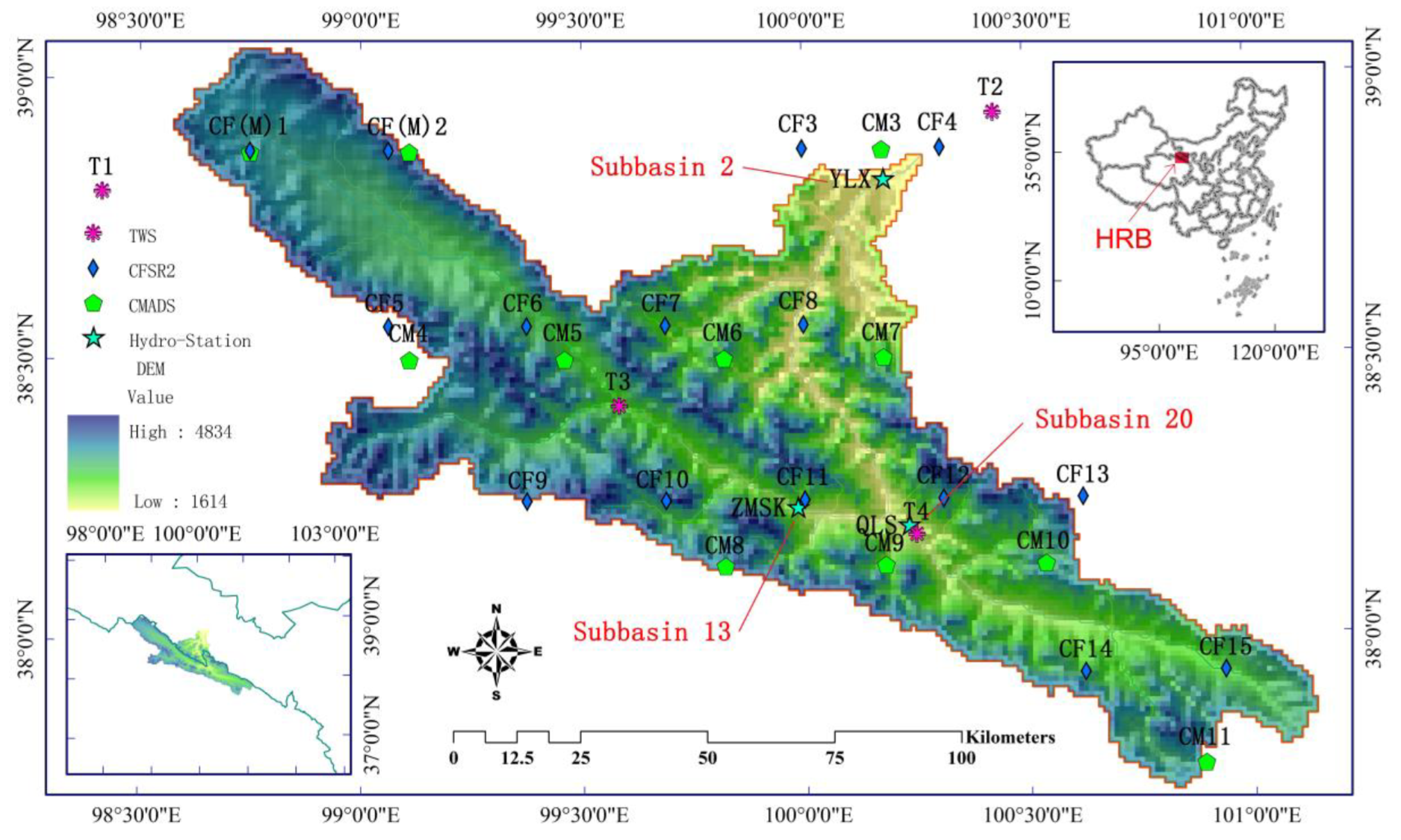
2. Study Region
3. Materials and Methods
3.1. Land Surface Input Data
3.1.1. Digital Elevation Model
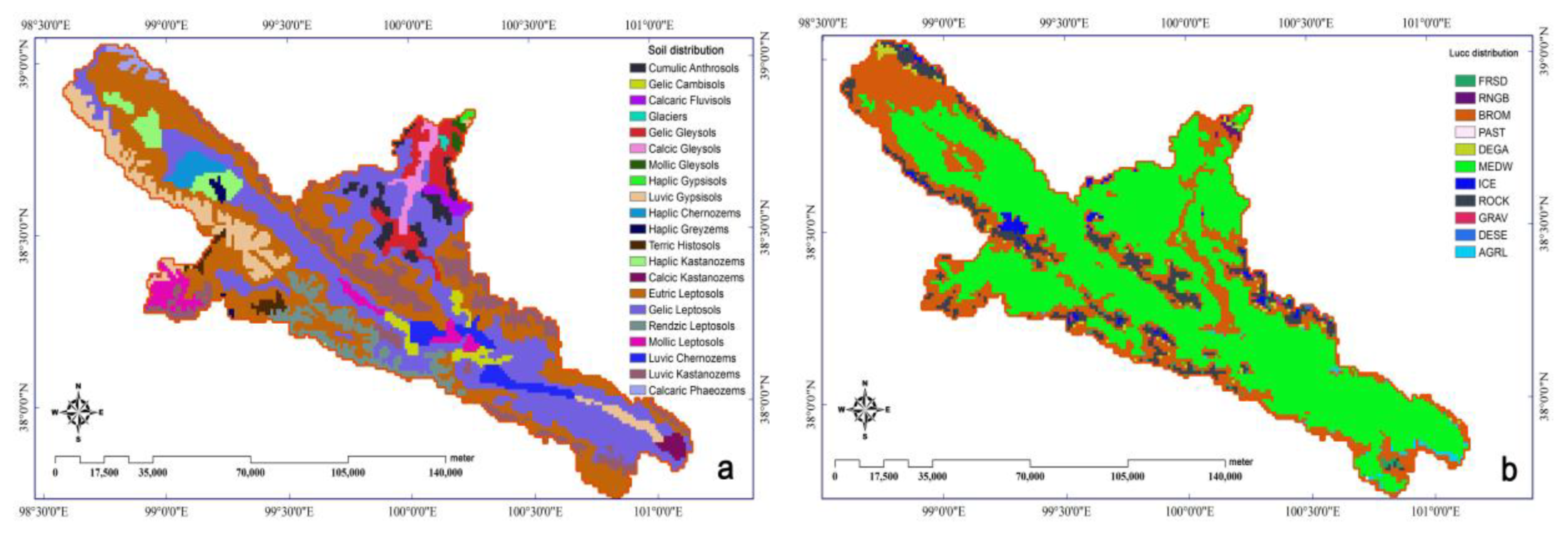
3.1.2. Soil Distribution and Land Use Data
3.2. Hydrological Verification Data
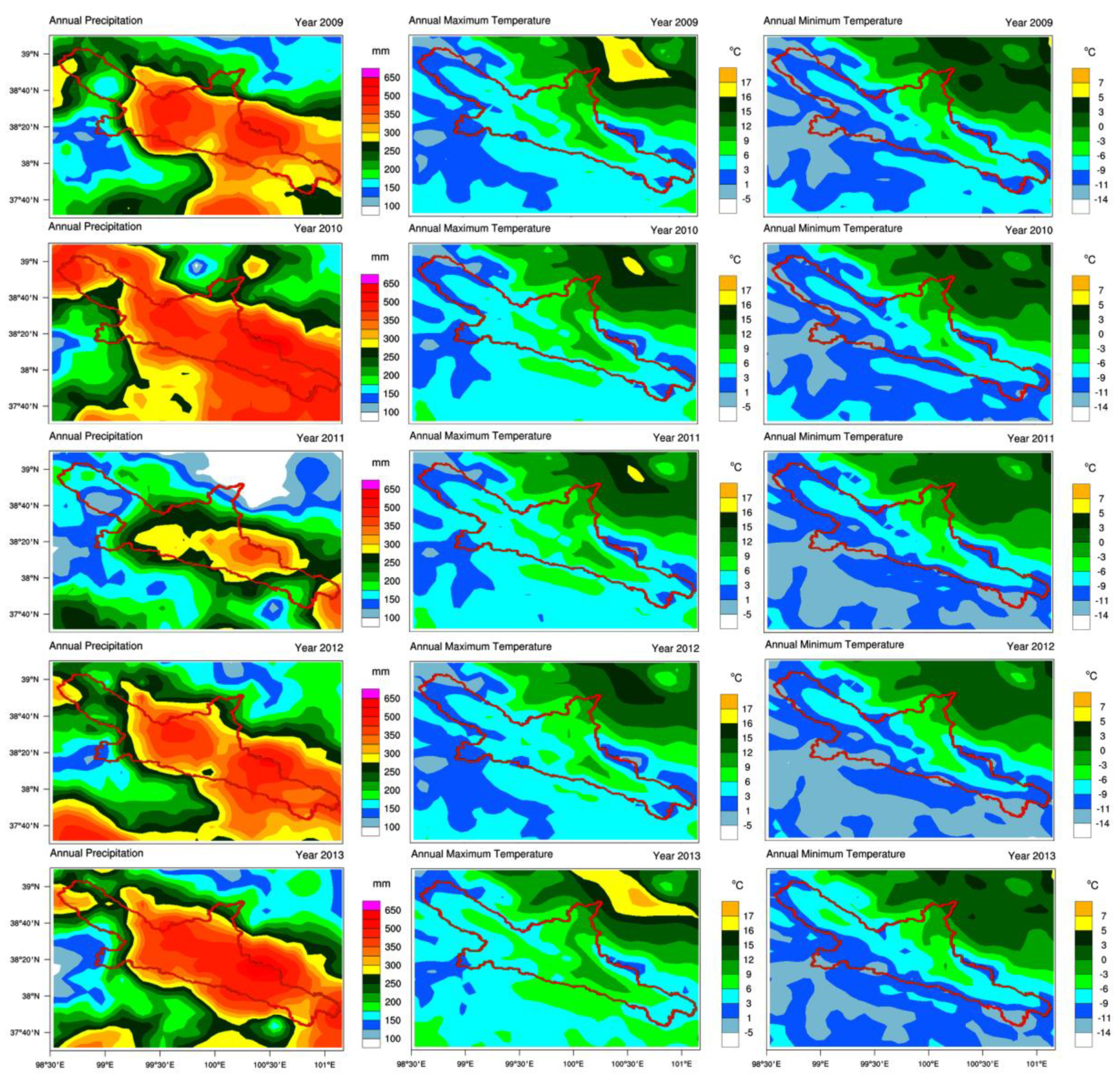
3.3. Atmospheric Forcing Input Data
3.3.1. TWS
3.3.2. CFSR
3.3.3. CMADS
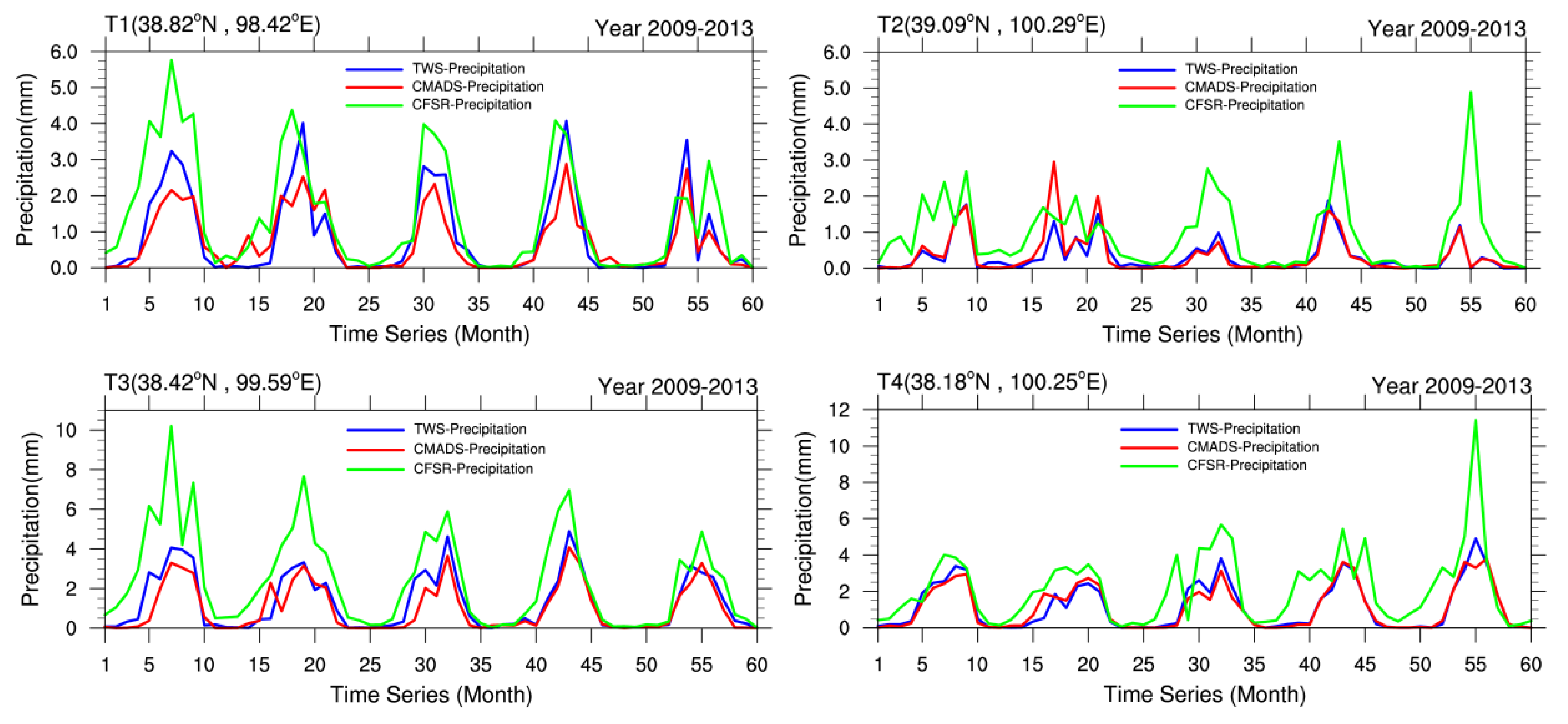
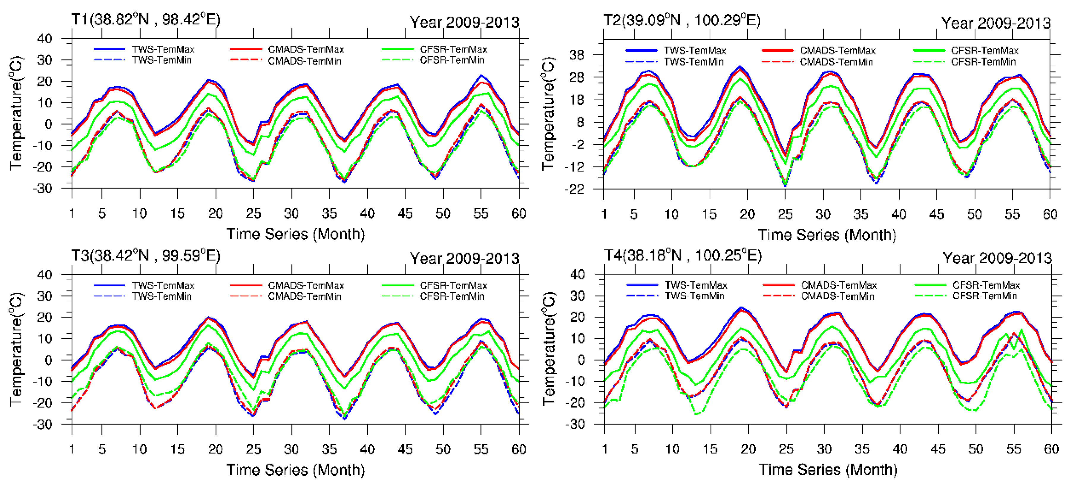
3.3.4. Evaluation of CFSR and CMADS Based on TWS
3.3.5. SWAT Model
Model Setting
Sensitivity Analysis
Model Calibration
Model Assessment
4. Results and Discussion
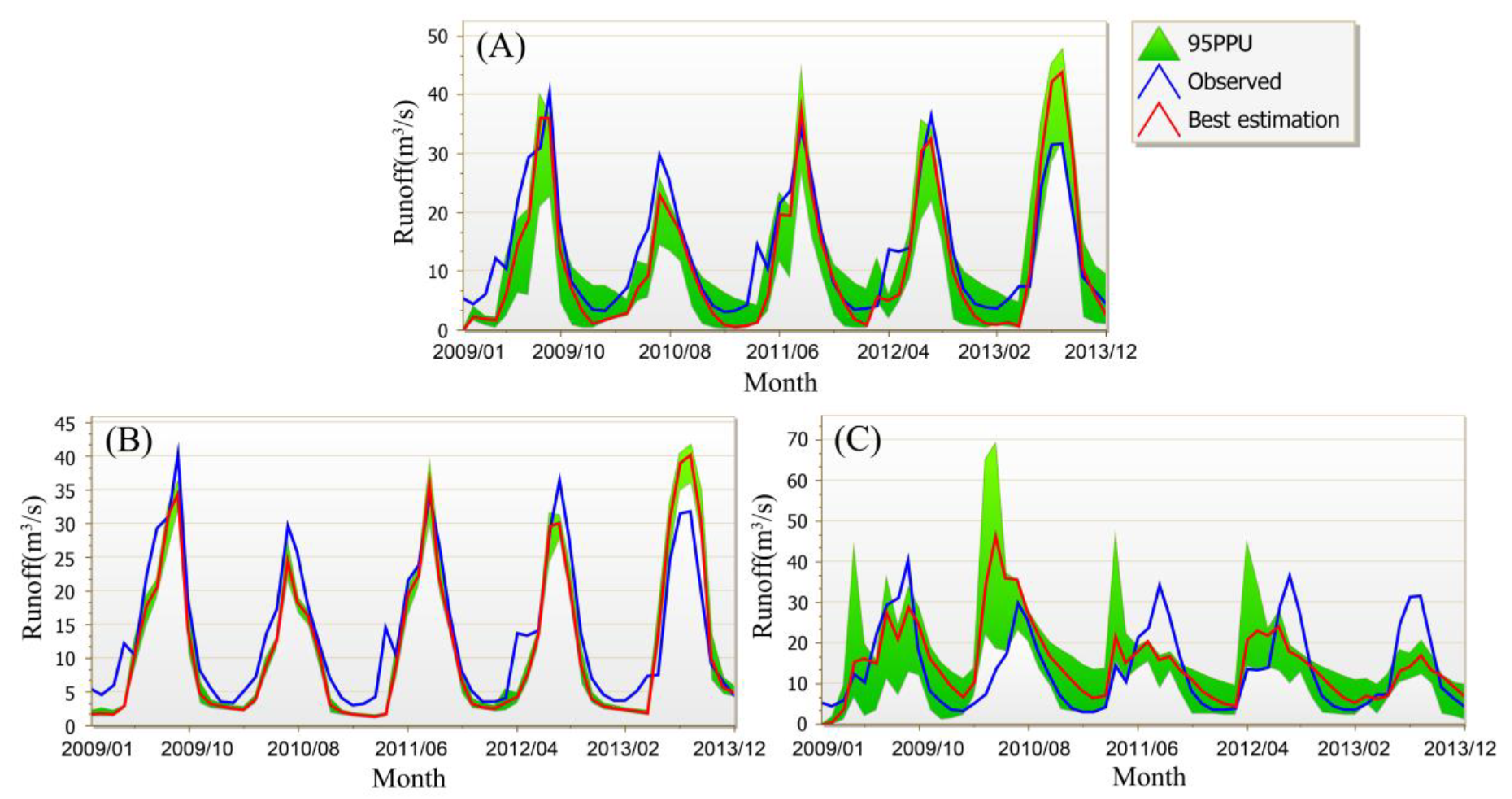
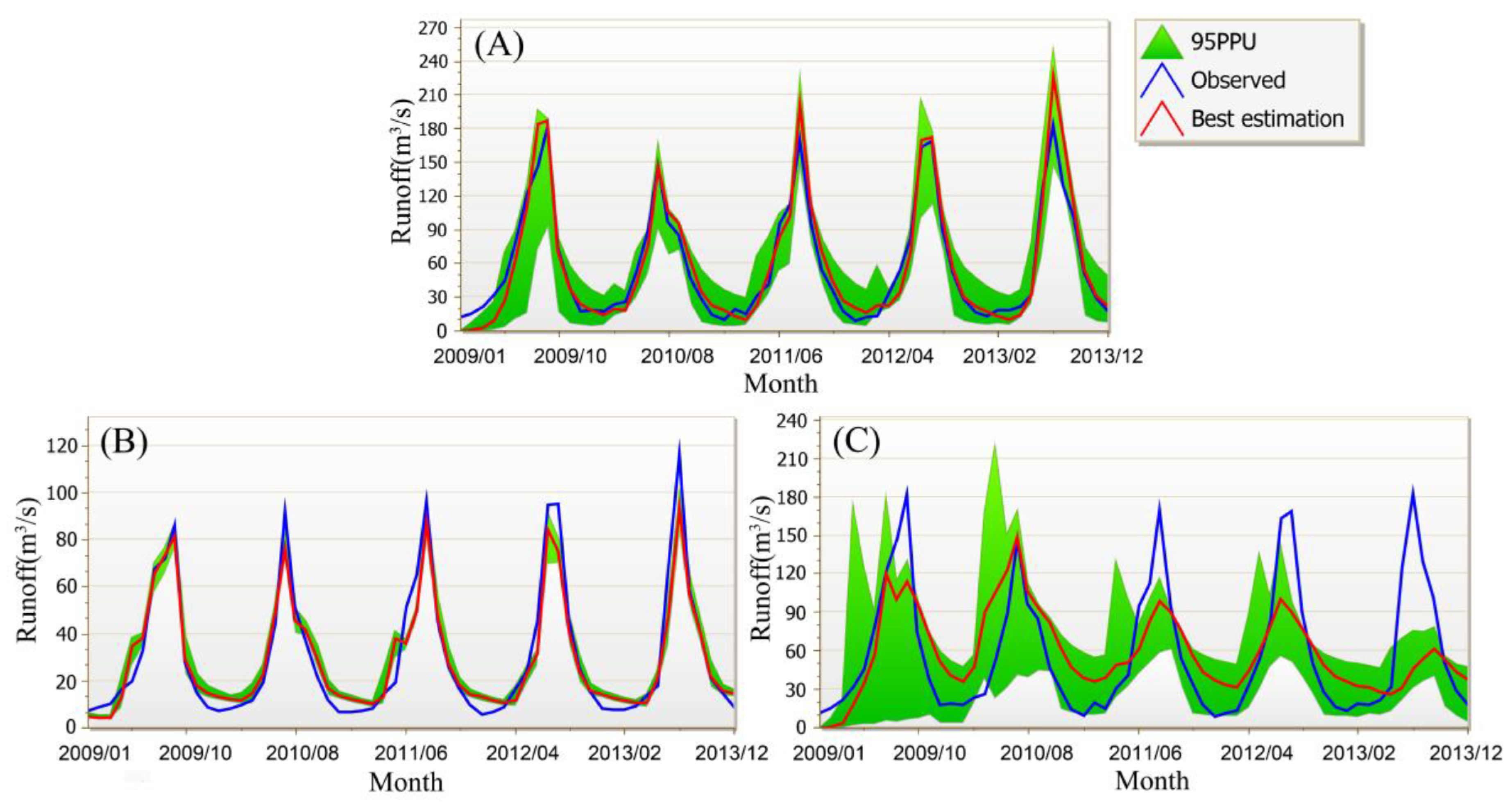
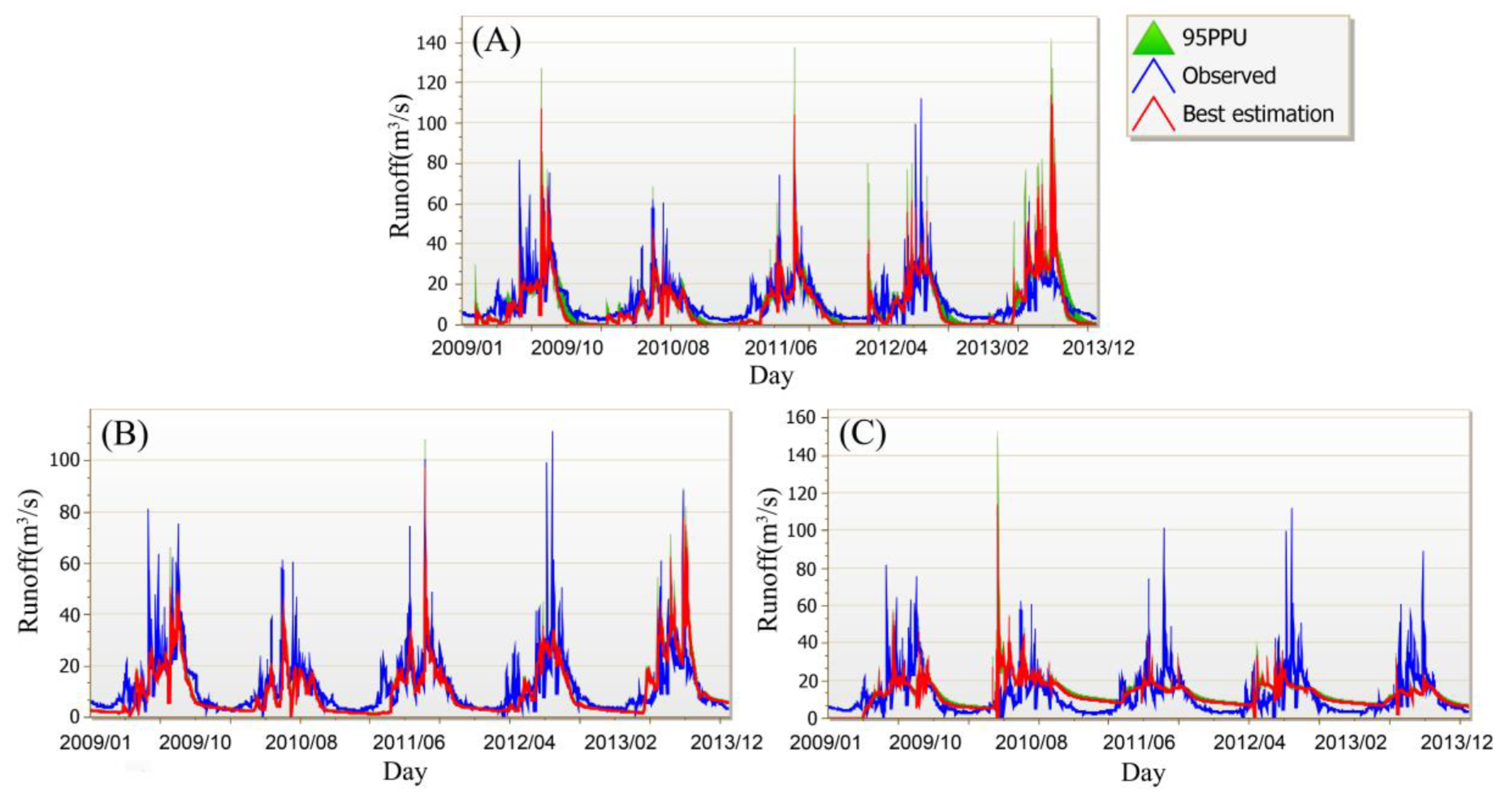
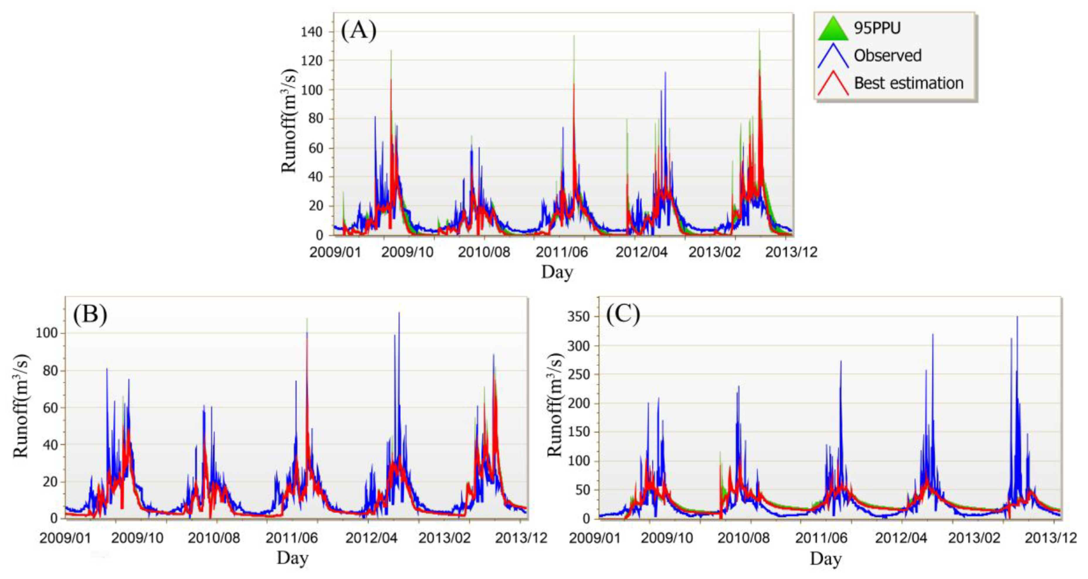
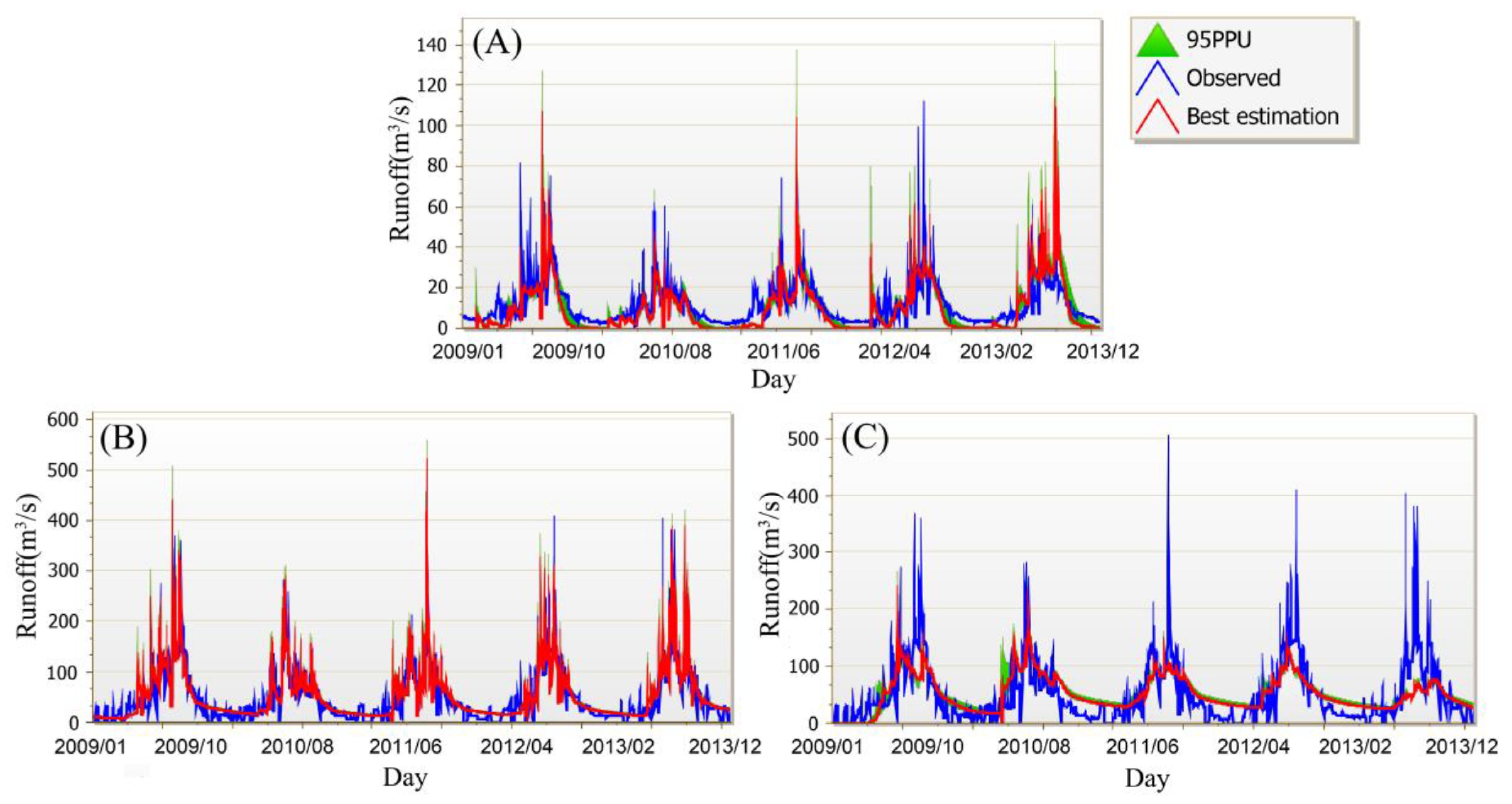
4.1. Daily- and Monthly-Scale Runoff Simulation Results by the Three Modes for Three Sub-Basins
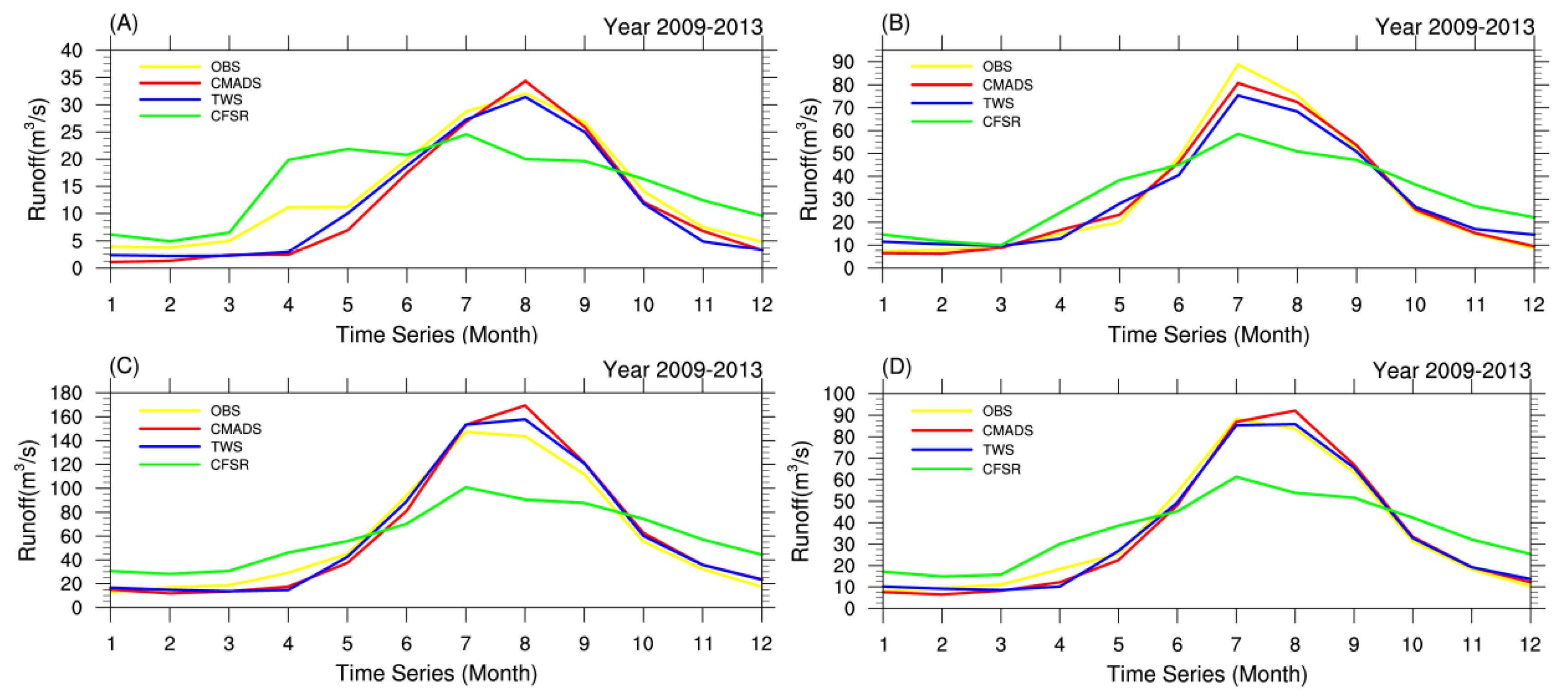
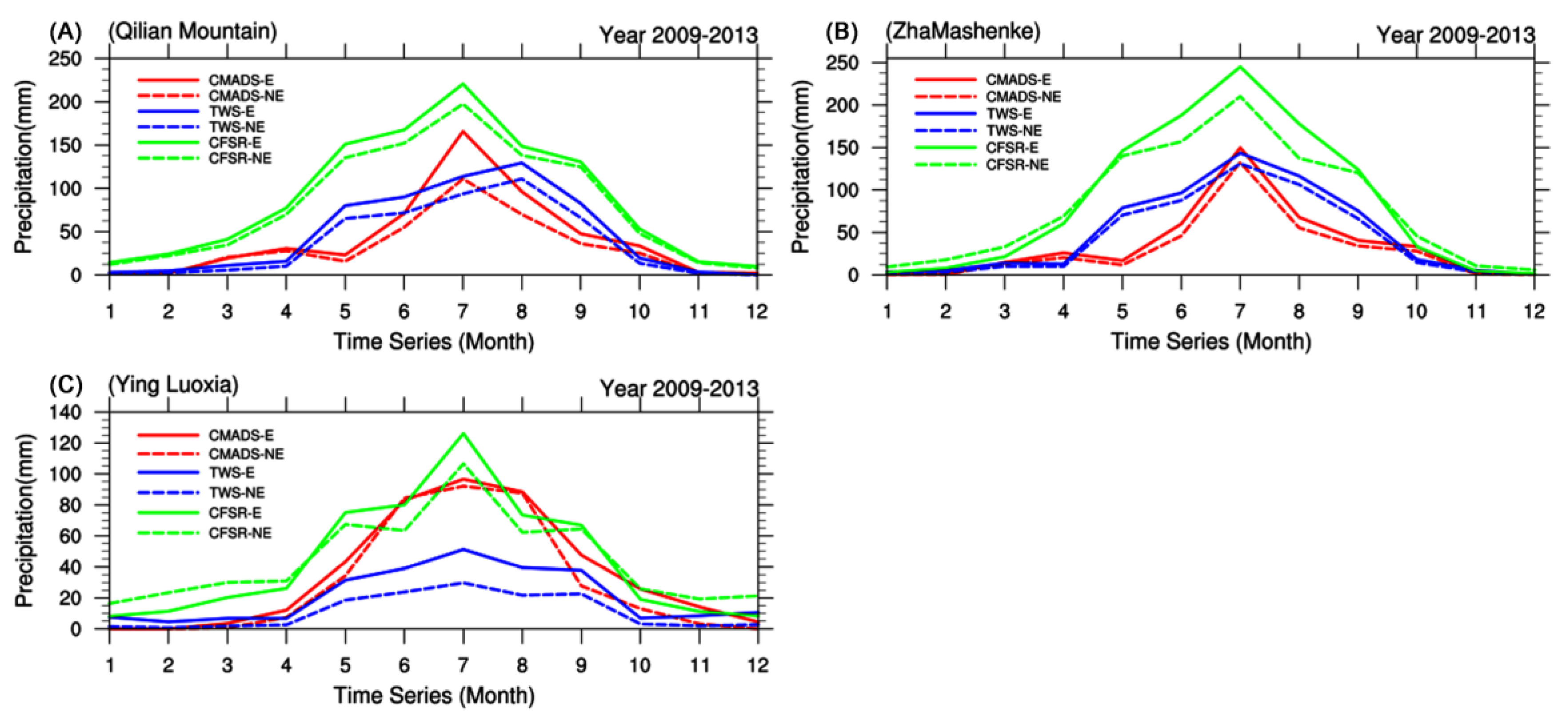
4.2. Five-Year Monthly-Scale Runoff Simulation Results for Three Sub-Basins
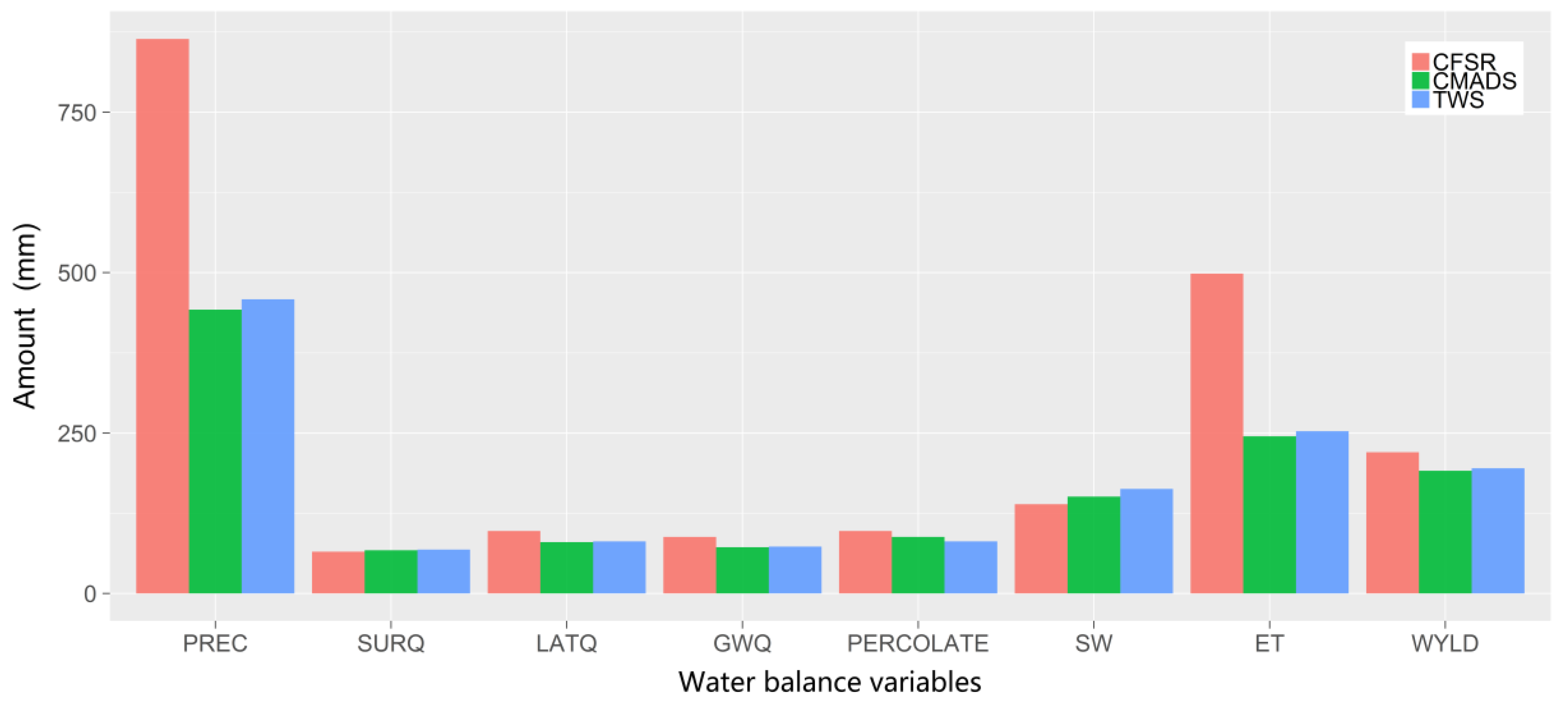
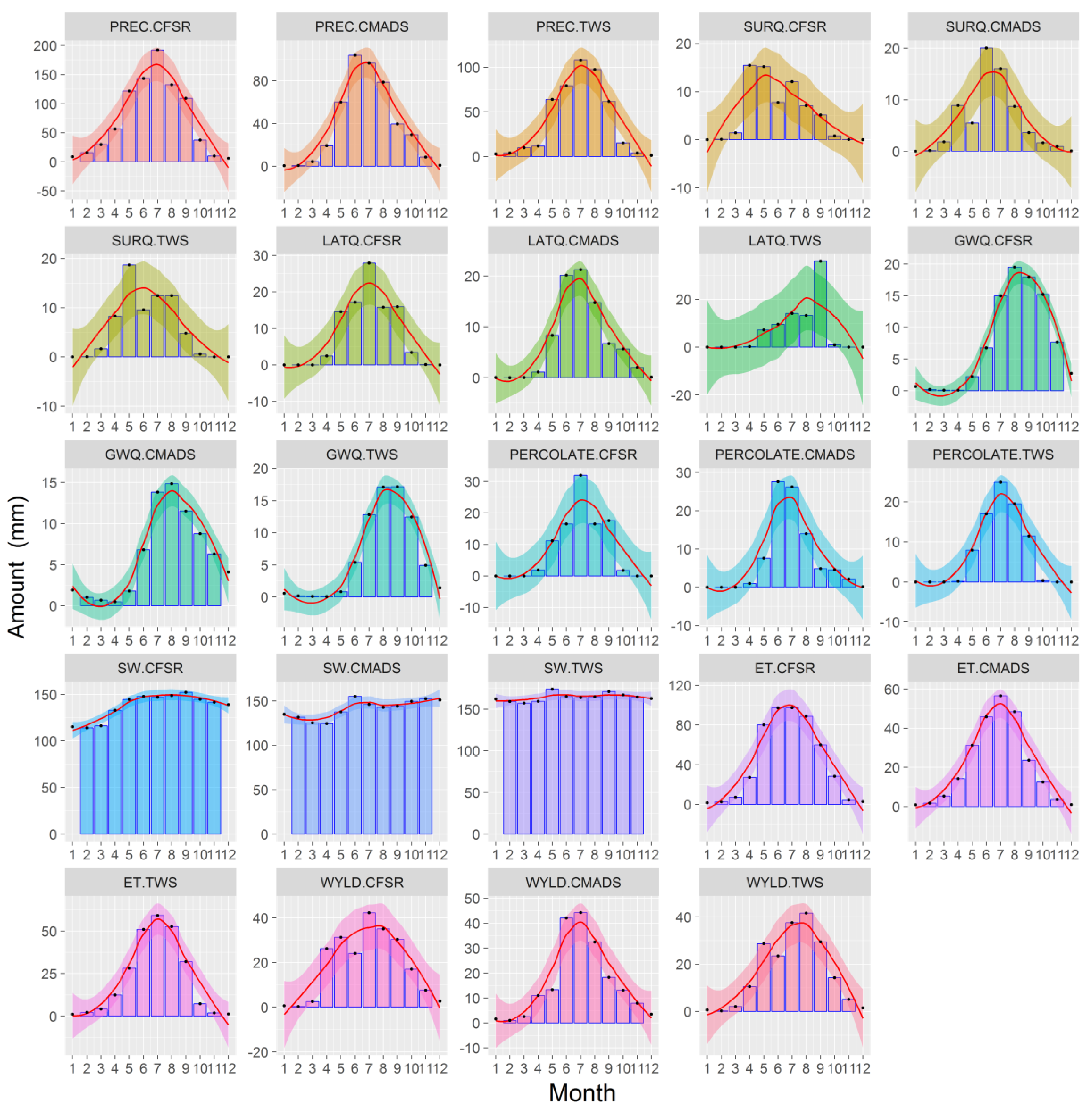
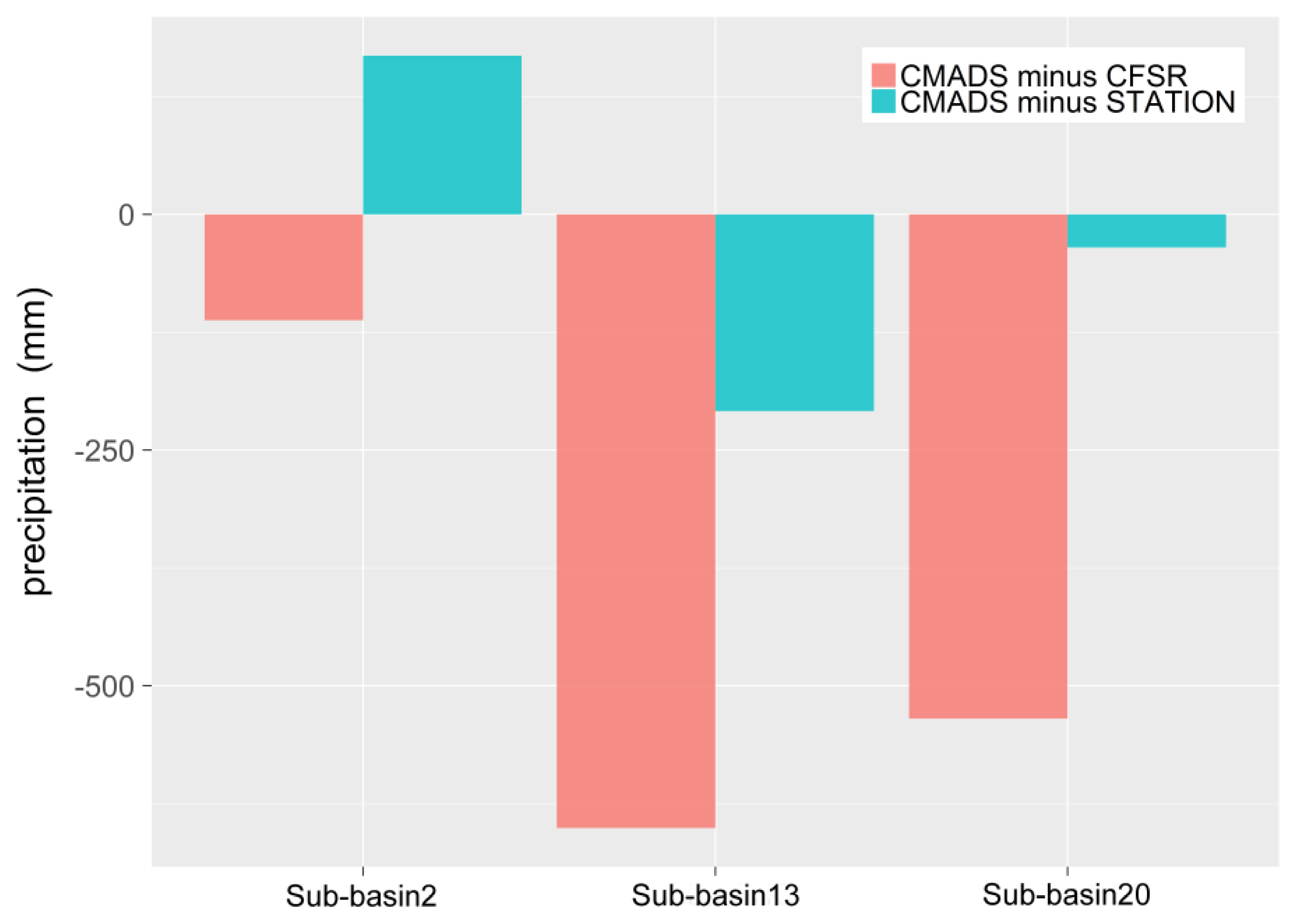
4.3. Differences Caused by Water Balance
5. Conclusions
- With regard to the accuracy of meteorological data, the results obtained using the CMADS dataset generally match observations obtained at automatic stations in China. The goodness of fit between CMADS and TWS was better than that between CFSR and TWS.
- The runoff results obtained by the CMADS-driven SWAT model almost perfectly reproduce historical runoff data. This excellent performance is not only reflected in the runoff simulation evaluation indicators, but also found through the analysis of 95PPU. CMADS outperforms TWS in terms of uncertainty, and CFSR performs worst. In the best simulation, CMADS data is slightly better than TWS, and CFSR performance is the worst. This excellent performance by CMADS is similar on both monthly and daily scales, while CFSR shows poor simulation ability due to the overestimation of summer precipitation.
- The CMADS + SWAT mode has a greater ability to reproduce water balance than the other two modes. However, because of the complexity of surface processes in the basin, further investigation is needed.
- Overestimation of CFSR precipitation results in a greater error impact on the uncertainty output of the model, whereas the performances of CMADS and TWS are more similar when driving the SWAT model.
Author Contributions
Funding
Conflicts of Interest
Abbreviations
| HRB | Heihe River Basin |
| SWAT | Soil and Water Assessment Tool |
| CMADS | China Meteorological Assimilation Driving Datasets for the SWAT model |
| CFSR | Climate Forecast System Reanalysis |
| TWS | Traditional meteorological Station |
| CMADS+SWAT | SWAT Model Driven by CMADS |
| CFSR+SWAT | SWAT Model Driven by CFSR |
| TWS+SWAT | SWAT Model Driven by TWS |
| NCEP | National Centers for Environmental Prediction |
| NCAR | National Center for Atmospheric Research |
| ECMWF | European Centre for Medium-Range Weather Forecast |
| ERA-Interim | ECMWF Reanalysis-Interim |
| ERA-15 | ECMWF Reanalysis-15 |
| ERA-40 | ECMWF Reanalysis-40 |
| MERRA | Modern Era Retrospective-Analysis for Research and Applications |
| NASA | National Aeronautics and Space Administration |
| EnKF | Ensemble Kalman Filter |
| IFS | Integration Forecasting System |
| MOM4 | Modular Ocean Model Version 4 |
| 3DVAR | Three-Dimensional Variational Data Assimilation |
| GODAS | Global Ocean Data Assimilation System |
| GLDAS | Global Land Data Assimilation System |
| GEOS-5 | Goddard Earth Observing System, Version 5 |
| ADAS | Atmospheric Data Assimilation System |
| GIS | Geographic Information System |
| SiB | Simple Biosphere Mode |
| JRA-25 | Japanese 25-year ReAnalysis |
| JMA | Japan Meteorological Agency |
| JCDAS | JMA Climate Data Assimilation System |
| SAC-SMA | Sacramento Soil Moisture Accounting Model |
| TRMM | Tropical Rainfall Measuring Mission |
| IPCC | Intergovernmental Panel on Climate Change |
| GCMs | Global Climate Models |
| MC2 | Mesoscale Community Compressible |
| RegCM3 | Regional Climate Model, version 3 |
| CGIAR | Consultative Group on International Agricultural Research |
| CGIAR-CSI | CGIAR Consortium for Spatial Information |
| HRUs | Hydrological Response Units |
| GLC2000 | Global Land Cover Database for the year 2000 |
| WestDC | China West Data Centre |
| MEDW | Meadow |
| BROM | Meadow Bromegrass |
| ROCK | Bare Rocks |
| ICE | Ice |
| DEGA | Desert Grassland |
| AGRL | Farmland |
| FRSD | Needle-leaved Deciduous Forest |
| GRAV | Bravels |
| RNGB | Bush |
| DESE | Desert |
| PAST | Plain Grassland |
| DEM | Digital Elevation Model |
| SCS | Soil Conservation Service |
| SUFI-2 | Sequential Uncertainty Fitting |
| 95PPU | 95% prediction uncertainty |
| CN2.mgt | SCS runoff curve value |
| ALPHA_BF.gw | Baseflow factor |
| GW_DELAY.gw | Delay time (day) of aquifer replenishment |
| GWQMN.gw | Water level threshold (mm) of shallow aquifer when groundwater flowing into the main river channel |
| GW_REVAP.gw | Evaporation coefficient of groundwater |
| ESCO.hru | Compensation factor of soil evaporation |
| ALPHA_BNK.rte | Recession constant value of base flow |
| SFTMP | Average temperature (¡æ) at snowing days |
| PLAPS | Lapse rate of precipitation /(mm¡¤km-1) |
| SMFMN | Snowmelt factor at 21 December /mm¡¤(day-¡æ)-1 |
| SMFMX | Snowmelt factor at 21 June |
| TLAPS | Lapse rate of temperature |
| NSE | Nash-Sutcliffe Efficiency |
| R2 | Determination Efficiency |
| PREC | Precipitation |
| SURQ | Land surface runoff |
| LATQ | Side flow |
| GWQ | Subsurface flow |
| PERCOLATE | Lateral seepage flow |
| SW | Soil water |
| ET | Actual evaporation |
| WYLD | Runoff |
References
- Collick, A.S.; Easton, Z.M.; Ashagrie, T. A simple semi-distributed water balance model for the Ethiopian highlands. Hydrol. Process. 2009, 23, 3718–3727. [Google Scholar] [CrossRef]
- Lyu, H.M.; Shen, L.S.; Yang, J.; Yin, Z.Y. Scenario-based inundation analysis of metro systems: A case study in Shanghai. Hydrol. Earth Syst. Sci. Discuss. 2019. In review. [Google Scholar] [CrossRef]
- Kim, U.; Kaluarachchi, J.J.; Smakhtin, V.U. Generation of monthly precipitation under climate change for the Upper Blue Nile River Basin, Ethiopia. J. Am. Water Resour. Assoc. 2008, 44, 1231–1247. [Google Scholar] [CrossRef]
- Muluneh, A.M.; Anders, W.; Bijan, D. Hydrological modelling of Ethiopian catchments using limited data. Hydrol. Process. 2009, 23, 3401–3408. [Google Scholar]
- Assefa, M.M.; Wossenu, A.; Tibebe, D.; Wang, X. Low and high flow analyses and wavelet application for characterization of the Blue Nile River system. Hydrol. Process. 2010, 252, 241–252. [Google Scholar]
- Neitsch, S.L.; Arnold, J.G.; Kiniry, J.R. Soil and Water Assessment Tool Theoretical Documentation, version 2005; Grassland Soil and Water Research Laboratory, Agricultural Research Service, Blackland Research Center, Texas Agricultural Experiment Station: Temple, TX, USA, 2012. [Google Scholar]
- Zhang, Q.; Heiner, K.; Karin, H. How well do reanalyses represent the southern African precipitation? Clim. Dyn. 2013, 40, 951–962. [Google Scholar] [CrossRef]
- NCEP Climate Forecast System Reanalysis (CFSR) Selected Hourly Time-Series Products, January 1979 to December 2009. Available online: https:// rda.ucar.edu/ datasets/ ds093.1/ docs/ CFSR – Hourly - Timeseries.pdf (accessed on 2 December 2010).
- Trenberth, K.E.; Anthes, R.A.; Belward, A. 2013 Challenges of A Sustained Climate Observing System; Springer: Berlin, Germany.
- Saha, S.; Nadiga, S.; Thiaw, C.; Wang, J.; Wang, W.; Zhang, Q.; van den Dool, H.M.; Pan, H.-L.; Moorthi, S.; Stokes, D.; et al. The NCEP climate forecast system. J. Clim. 2006, 19, 3483–3517. [Google Scholar] [CrossRef]
- Kanamitsu, M.; Ebisuzaki, W.; Woollen, J. NCEP-DEO AMIP-II reanalysis (R-2). Bul. Aymos. Met. Soc. 2002, 83, 1631–1643. [Google Scholar] [CrossRef]
- Dee, D.P.; Uppala, S.M.; Simmons, A.J. The ERA-Interim reanalysis: Configuration and performance of the data assimilation system. Q. J. R. Meteorol. Soc. 2011, 137, 553–597. [Google Scholar] [CrossRef]
- Gibson, J.K.; Allberg, K.; Uppala, P.; Nomura, S. ERA description. In ECMWF ERA-15 Project Report Series, No.1; European Centre for Medium-Range Weather Forecasts: Shinfield, UK, 1997; Available online: www.ecmwf.int/publications (accessed on 1 January 1999).
- Uppala, S.M.; Kllberg, P.W.; Simmons, A.J. The ERA-40 re-analysis. Q. J. R. Meteorol. Soc. 2005, 131, 2961–3012. [Google Scholar] [CrossRef]
- Rienecker, M.M. NASA’s modern-era retrospective analysis for research and applications. J. Clim. 2011, 24, 3624–3648. [Google Scholar] [CrossRef]
- Najafi, M.R.; Moradkhani, H.; Piechota, T.C. Ensemble streamflow prediction: Climate signal weighting methods vs. climate forecast system reanalysis. J. Hydrol. 2012, 442, 105–116. [Google Scholar] [CrossRef]
- Fuka, D.R.; Walter, M.T.; MacAlister, C. Using the climate forecast system reanalysis as weather input data for watershed models. Hydrol. Process. 2014, 28, 5613–5623. [Google Scholar] [CrossRef]
- Smith, R.A.; Kummerow, C.D. A comparison of in situ, reanalysis, and satellite water budgets over the Upper Colorado River Basin. J. Hydrometeorol. 2013, 14, 888–905. [Google Scholar] [CrossRef]
- David, A.L.; Gabriele, V.; Richard, P.A.; Eric, F.W.; Andrew, J.W. The detection of atmospheric rivers in atmospheric reanalyses and their links to British winter floods and the large-scale climatic circulation. J. Geophys. Res. 2012, 117. [Google Scholar] [CrossRef]
- Quadro, M.F.; Berbery, E.H.; Dias, M.A.F.S. The atmospheric water cycle over South America as seen in the new generation of global reanalyses. In AIP Conference Proceedings; American Institute of Physics: College Park, MD, USA, 2013; Volume 732, pp. 732–735. [Google Scholar]
- Wu, W.; Chen, J.L.; Huang, R.H. Water budgets of tropical cyclones: Three case studies. Adv. Atmos. Sci. 2013, 30, 468–484. [Google Scholar] [CrossRef]
- Takacs, L.L.; Molod, A.; Wang, T. Documentation of the Goddard Earth Observing System (GEOS) General Circulation Model; version 1; NASA Technical Memorandum: Washington, DC, USA, 1994. Available online: https://gmao.gsfc.nasa.gov/pubs/docs/Takacs126.pdf (accessed on 10 December 2004).
- Schubert, S.D.; Park, C.K.; Wu, C.Y. A multi-year assimilation with the GEOS-1 system: overview and results. In NASA Technical Report Series on Global Modeling and Data Assimilation; Suarea, M.J., Ed.; NASA: Washington, DC, USA, 1995. [Google Scholar]
- Simmons, A.J.; Gibson, J.K. The ERA-40 Project Plan. ECMWF Re-Analysis Project Report Series No. 1. 2000. Available online: https://www.ecmwf.int/sites/default/files/elibrary/2000/12272-era-40-project-plan.pdf (accessed on 31 March 2000).
- Kazutoshi, O.; Junichi, T.; Hiroshi, K.; Masami, S. The JRA-25 reanalysis. J. Meteorol. Soc. Jpn. 2007, 85, 369–432. [Google Scholar]
- Simmons, A.; Uppala, S.; Dee, D.; Kobayashi, S. ERA-Interim: New ECMWF Reanalysis Products from 1989 Onwards. ECMWF Newsletter, No. 110; ECMWF: Reading, UK, 2007; Volume 110, pp. 25–35. [Google Scholar]
- Ebita, A. The Japanese 55-year reanalysis “JRA-55”: An interim report. Sola 2011, 7, 149–152. [Google Scholar] [CrossRef]
- Compo, G.P.; Whitaker, J.S.; Sardeshmukh, P.D.; Matsui, N.; Allan, R.J.; Yin, X.; Gleason, B.E.; Vose, R.S.; Rutledge, G.; Bessemoulin, P.; et al. The twentieth century reanalysis project. Q. J. R. Meteorol. Soc. 2011, 137, 1–28. [Google Scholar] [CrossRef]
- Smirnov, A.; Holben, B.N.; Slutsker, I.; Giles, D.M.; McClain, C.R.; Eck, T.F.; Sakerin, S.M.; Macke, A.; Croot, P.; Zibordi, G.; et al. Maritime aerosol network as a component of aerosol robotic network. J. Geophys. Res. 2009, 114. [Google Scholar] [CrossRef]
- Olaf, S.; Johannes, F.; Antje, I.; Johannes, W.K.; Martin, G.S. Global reactive gases forecasts and reanalysis in the MACC project. J. Integr. Environ. Sci. 2012, 9, 57–70. [Google Scholar] [Green Version]
- Zhao, T.B.; Xu, Z.B. Preliminary comparison and analysis between ERA-40, NCEP-2 reanalysis and observations over China. Clim. Environ. Res. 2006, 11, 14–32. [Google Scholar]
- Huang, G. The assessment and difference of the interdecadal variations of climate change in northern part of China with the NCEP/NCAR and ERA-40 reanalysis data. Clim. Environ. Res. 2006, 11, 310–320. [Google Scholar]
- Higgins, R.W.; Kousky, V.E.; Silva, V.B.; Becker, E.; Xie, P. Intercomparison of daily precipitation statistics over the United States in observations and in NCEP reanalysis products. J. Clim. 2010, 23, 4637–4650. [Google Scholar] [CrossRef]
- Silva, V.B.; Kousky, V.E.; Higgins, R.W. Daily precipitation statistics for South America: An intercomparison between NCEP reanalyses and observations. J. Hydrometeorol. 2011, 12, 101–117. [Google Scholar] [CrossRef]
- Gerald, A.M.; Curt, C.; Thomas, D.; Mojib, L.; Bryant, M.; John, F.B.; Ronald, J.S.; Karl, E.T. The WCRP CMIP3 multimode dataset: A new era in climate change research. Bull. Am. Meteorol. Soc. 2007, 88, 1383–1394. [Google Scholar]
- Wood, A.W.; Leung, L.R.; Sridhar, V.; Lettenmaier, D.P. Hydrologic implications of dynamical and statistical approaches to downscale climate model outputs. Clim. Chang. 2004, 62, 189–216. [Google Scholar] [CrossRef]
- Lu, G.H.; Wu, Z.Y.; Lei, W.; Zhang, J.Y. Application of a coupled atmospheric-hydrological modeling system to real-time flood forecast. Adv. Water Sci. 2007, 16, 847–852. [Google Scholar]
- Wang, C. The Impact Climate Change on Runoff in Qilian Mountain—A Case Study in Upper Reaches of Heihe River Basin. Ph.D. Thesis, Lanzhou University, Lanzhou, China, 2010. [Google Scholar]
- Jeremy, P. Examples of simulations with the latest version of the RegCM. A little taste of the RegCM. Examples of simulations. Europe East Asia simulation of the monsoon west Africa simulation of the monsoon sensitivity to the convective closure assumption North America—PowerPoint PPT presentation. In Proceedings of the ITCP Workshop on the Theory and Use of Regional Climate Model, Trieste, Italy, 26 May–6 June 2003. [Google Scholar]
- Fischer, G.; Nachtergaele, F.; Prieler, S.; van Velthuizen, H.T.; Verelst, L.; Wiberg, D. Global Agro-Ecological Zones Assessment for Agriculture (GAEZ 2008); IIASA: Laxenburg, Austria; FAO: Rome, Italy, 2008. [Google Scholar]
- Zhang, Q.; Zhang, X. Impacts of predictor variables and species models on simulating Tamarix ramosissima distribution in Tarim Basin, northwestern China. J. Plant Ecol. 2012, 5, 337–345. [Google Scholar] [CrossRef]
- Liu, S.Y.; Yao, X.J.; Guo, W.Q. The contemporary glaciers in China based on the Second Chinese Glacier Inventory. Acta Geogr. Sin. 2015, 70, 3–16. [Google Scholar]
- Guo, W.Q.; Liu, S.Y.; Yao, X.J. The Second Glacier Inventory Dataset of China; Cold and Arid Regions Science Data Center at Lanzhou: Lanzhou, China, 2014. [Google Scholar]
- Jafet, C.M.; Alexander, J.B.; Bernhard, W.; Hong, Y. Improved SWAT model performance with time-dynamic voronoi tessellation of climatic input data in Southern Africa. J. Am. Water Resour. Assoc. 2012, 48, 480–493. [Google Scholar]
- Meng, X.Y.; Wang, H. Investigating spatiotemporal changes of the land-surface processes in Xinjiang using high-resolution CLM3.5 and CLDAS: Soil temperature. Sci. Rep. 2017, 7, 13286. [Google Scholar] [CrossRef] [PubMed]
- Meng, X.Y.; Wang, H.; Chen, J. Profound impacts of the China meteorological assimilation dataset for SWAT model (CMADS). Water 2019, 11, 832. [Google Scholar] [CrossRef]
- Meng, X.Y.; Wang, H.; Shi, C.; Wu, Y.; Ji, X. Establishment and evaluation of the China meteorological assimilation driving datasets for the SWAT model (CMADS). Water 2018, 10, 1555. [Google Scholar] [CrossRef]
- Meng, X.Y.; Wang, H. Significance of the China meteorological assimilation driving datasets for the SWAT model (CMADS) of East Asia. Water 2017, 9, 765. [Google Scholar] [CrossRef]
- Meng, X.Y.; Wang, H.; Lei, X.H.; Cai, S.Y.; Wu, H.J. Hydrological modeling in the Manas River Basin using soil and water assessment tool driven by CMADS. Teh. Vjesn. 2017, 24, 525–534. [Google Scholar]
- Cao, Y.; Zhang, J.; Yang, M. Application of SWAT model with CMADS data to estimate hydrological elements and parameter uncertainty based on SUFI-2 algorithm in the Lijiang River Basin, China. Water 2018, 10, 742. [Google Scholar] [CrossRef]
- Liu, J.; Shanguan, D.; Liu, S.; Ding, Y. Evaluation and hydrological simulation of CMADS and CFSR reanalysis datasets in the Qinghai-Tibet Plateau. Water 2018, 10, 513. [Google Scholar] [CrossRef]
- Shao, G.; Guan, Y.; Zhang, D.; Yu, B.; Zhu, J. The impacts of climate variability and land use change on streamflow in the Hailiutu River Basin. Water 2018, 10, 814. [Google Scholar] [CrossRef]
- Vu, T.T.; Li, L.; Jun, K.S. Evaluation of multi satellite precipitation products for streamflow simulations: A case study for the Han River Basin in the Korean Peninsula, East Asia. Water 2018, 10, 642. [Google Scholar] [CrossRef]
- Zhao, F.; Wu, Y. Parameter uncertainty analysis of the SWAT model in a mountain-loess transitional watershed on the Chinese Loess Plateau. Water 2018, 10, 690. [Google Scholar] [CrossRef]
- Zhou, S.; Wang, Y.; Chang, J.; Guo, A.; Li, Z. Investigating the dynamic influence of hydrological model parameters on runoff simulation using sequential uncertainty fitting-2-based multilevel-factorial-analysis method. Water 2018, 10, 1177. [Google Scholar] [CrossRef]
- Gao, X.; Zhu, Q.; Yang, Z.; Wang, H. Evaluation and hydrological application of CMADS against TRMM 3B42V7, PERSIANN-CDR, NCEP-CFSR, and gauge-based datasets in Xiang River Basin of China. Water 2018, 10, 1225. [Google Scholar] [CrossRef]
- Tian, Y.; Zhang, K.; Xu, Y.-P.; Gao, X.; Wang, J. Evaluation of potential evapo-transpiration based on CMADS reanalysis dataset over China. Water 2018, 10, 1126. [Google Scholar] [CrossRef]
- Qin, G.; Liu, J.; Wang, T.; Xu, S.; Su, G. An integrated methodology to analyze the total nitrogen accumulation in a drinking water reservoir based on the SWAT model driven by CMADS: A case study of the Biliuhe Reservoir in Northeast China. Water 2018, 10, 1535. [Google Scholar] [CrossRef]
- Guo, B.; Zhang, J.; Xu, T.; Croke, B.; Jakeman, A.; Song, Y.; Yang, Q.; Lei, X.; Liao, W. Applicability assessment and uncertainty analysis of multi-precipitation datasets for the simulation of hydrologic models. Water 2018, 10, 1611. [Google Scholar] [CrossRef]
- Dong, N.P.; Yang, M.X.; Meng, X.Y.; Liu, X. CMADS-driven simulation and analysis of reservoir impacts on the streamflow with a simple statistical approach. Water 2018, 11, 178. [Google Scholar] [CrossRef]
- Guo, D.; Wang, H.; Zhang, X.; Liu, G. Evaluation and analysis of grid precipitation fusion products in Jinsha River Basin based on China meteorological assimilation datasets for the SWAT Model. Water 2019, 11, 253. [Google Scholar] [CrossRef]
- Yuan, Z.; Xu, J.; Meng, X.; Wang, Y.; Yan, B. Impact of climate variability on blue and green water flows in the Erhai Lake Basin of Southwest China. Water 2019, 11, 424. [Google Scholar] [CrossRef]
- Li, Y.; Wang, Y.; Zheng, J.; Yang, M. Investigating Spatial and Temporal Variation of Hydrological Processes in Western China Driven by CMADS. Water 2019, 11, 435. [Google Scholar] [CrossRef]
- Zhao, X.; Xu, S.; Liu, T.; Qiu, P.; Qin, G. moisture distribution in sloping black soil farmland during the freeze–thaw period in northeastern China. Water 2019, 11, 536. [Google Scholar] [CrossRef]
- Liu, X.; Yang, M.; Meng, X.; Wen, F.; Sun, G. Assessing the impact of reservoir parameters on runoff in the Yalong River Basin using the SWAT Model. Water 2019, 11, 643. [Google Scholar] [CrossRef]
- Zhang, L.; Meng, X.; Wang, H.; Yang, M. Simulated runoff and sediment yield responses to land-use change using the SWAT model in northeast China. Water 2019, 11, 915. [Google Scholar] [CrossRef]
- Abbaspour, K.C.; Vejdani, M.; Haghighat, S. 2007b SWAT-CUP calibration and uncertainty programs for SWAT. In MODSIM 2007b International Congress on Modelling and Simulation; Oxley, L., Kulasiri, D., Eds.; Modelling and Simulation Society of Australia and New Zealand Christchurch: Australiasia, New Zealand, 2007; pp. 1596–1602. [Google Scholar]
- Abbaspour, K.C.; Johnson, C.A. Estimating uncertain flow and transport parameters using a sequential uncertainty fitting procedure. Vadouse Zone J. 2004, 3, 1340–1352. [Google Scholar] [CrossRef]
- Abbaspour, K.C.; Yang, J.; Maximov, I.; Siber, R.; Bogner, K.; Mieleitner, J.; Zobris, J.T.; Srinivasan, R. Modelling hydrology and water quality in the pre-alpine/alpine Thur watershed using SWAT. J. Hydrol. 2007, 333, 413–430. [Google Scholar] [CrossRef]
- Abbaspour, K.C. Swat-Cup2: SWAT Calibration and Uncertainty Programs Manual Version 2, Department of Systems Analysis; Integrated Assessment and Modelling (SIAM), Eawag, Swiss Federal Institute of Aquatic Science and Technology: Duebendorf, Switzerland, 2011; p. 106. [Google Scholar]
- Wu, Y.; Liu, S.; Huang, Z.; Yan, W. Parameter optimization, sensitivity and uncertainty analysis of an ecosystem model at a forest flux tower site in the United States. J. Adv. Model. Earth Syst. 2014, 6, 405–419. [Google Scholar] [CrossRef]
- Wu, Y.; Liu, S. Improvement of the R-SWAT-FME framework to support multiple variables and multi-objective functions. Sci. Total Environ. 2014, 466, 455–466. [Google Scholar] [CrossRef]
- Tu, M.C.; Smith, P. Modeling pollutant buildup and washoff parameters for SWMM based on land use in a semiarid urban watershed. Water Air Soil Pollut. 2018, 229, 121. [Google Scholar] [CrossRef]
- Abbaspour, K.C.; Rouholahnejad, E.R.; Vaghefi, S.; Srinivasan, R.; Yang, H.; Kløve, B. A continental-scale hydrology and water quality model for Europe: Calibration and uncertainty of a high-resolution large-scale SWAT model. J. Hydrol. 2015, 524, 733–752. [Google Scholar] [CrossRef] [Green Version]
- Nash, J.E.; Sutcliffe, J.V. River flow forecasting through conceptual models: Part 1—A discussion of principles. J. Hydrol. 1970, 10, 282–290. [Google Scholar] [CrossRef]
- Schaefli, B.; Gupta, H.V. Do Nash values have value? Hydrol. Process. 2007, 21, 2075–2080. [Google Scholar] [CrossRef] [Green Version]
- Santhi, C.; Arnold, J.G.; Williams, J.R.; Dugas, W.A. Application of a watershed model to evaluate management efforts on point and nonpoint source pollution. Trans. ASAE. 2001, 44, 1559–1570. [Google Scholar] [CrossRef]
- Ahmad, H.M.; Sinclair, A.; Jamieson, R.; Madani, A.; Hebb, D.; Havard, P.; Yiridoe, E.K. Modeling sediment and nitrogen export from a rural watershed in Eastern Canada using the soil and water assessment tool. J. Environ. Qual. 2011, 40, 1182–1194. [Google Scholar] [CrossRef] [PubMed]
- Moriasi, D.N.; Arnold, J.G.; van Liew, M.W.; Bingner, R.L.; Harmel, R.D.; Veith, T.L. Model evaluation guidelines for systematic quantification of accuracy in watershed simulations. Trans. ASAE. 2012, 50, 885–900. [Google Scholar] [CrossRef]
- Yin, Z.L.; Xiao, H.L.; Zou, S.B.; Zhu, R.; Lu, Z.X.; Lan, Y.C.; Shen, Y.P. Progress of the research on hydrological simulation in the mainstream of the Heihe River, Qilian Mountains. J. Glaciol. Geocryol. 2013, 35, 438–446. [Google Scholar]


| Station Name | Nature Sub-Basin Area (km2) | Latitude (°) | Longitude (°) | Station Elevation (m) | Data Period (year) |
|---|---|---|---|---|---|
| Ying Luoxia | 243 | 38.82 | 100.18 | 1700.4 | 2009–2013 |
| Qilian Mountain | 310 | 38.20 | 100.23 | 3020.1 | 2009–2013 |
| ZhaMashenke | 126 | 38.23 | 99.98 | 2810.2 | 2009–2013 |
| Dataset | TWS | CFSR | CMADS |
|---|---|---|---|
| Elements | Daily average air pressure, daily average wind speed, daily average temperature, daily average relative humidity, daily maximum/minimum temperatures, 24 h precipitation, and sunshine duration | Daily accumulative precipitation, daily maximum/minimum temperatures, daily average wind speed, daily average relative humidity, and daily accumulative solar radiation | Daily maximum/minimum temperatures, daily average wind speed, daily average relative humidity, daily accumulative precipitation, and daily accumulative solar radiation |
| Data original spatial range | 4.00° N~53.31° N 73.40° E~135.05° E | Global | 0° N~65° N, 60° E~160° E |
| Data spatial range of this study | 37° N~39° N, 98° E~101° E | 24.5.00° N~57.00° N 44.00° E~129.00° E | 37.5° N~39.17° N, 98.5° E~101.17° E |
| Data timescale | 2008.1.1–2013.12.31 | 2008.1.1–2013.12.31 | 2008.1.1–2013.12.31 |
| Data original resolution ratio | / | 0.313°, 0.5°, 1.0°, 1.9°, 2.5° | 0.333°, 0.25°, 0.125°, 0.0625° |
| resolution ratio of this study | / | 0.313° | 0.333° |
| No. of stations imported by SWAT model | 4 (T1–T4) | 15 (CF1–CF15) | 11 (CM1–CM11) |
| Dataset Elements | TWS (T1) | TWS (T2) | TWS (T3) | TWS (T4) | ||||||||
|---|---|---|---|---|---|---|---|---|---|---|---|---|
| R2 | CORR | BIAS | R2 | CORR | BIAS | R2 | CORR | BIAS | R2 | CORR | BIAS | |
| CF-precipitation | 0.76 | 0.87 | 0.56 | 0.26 | 0.51 | 0.60 | 0.70 | 0.84 | 1.15 | 0.62 | 0.79 | 1.02 |
| CM-precipitation | 0.85 | 0.92 | −0.16 | 0.81 | 0.90 | 0.02 | 0.83 | 0.91 | −0.2 | 0.92 | 0.96 | −0.04 |
| CF-maximum temperature | 0.98 | 0.99 | −6.64 | 0.98 | 0.99 | −5.9 | 0.98 | 0.99 | −5.7 | 0.89 | 0.94 | −9.41 |
| CM-maximum temperature | 0.99 | 0.99 | −1.10 | 0.99 | 0.99 | −1.1 | 0.99 | 0.99 | −0.7 | 0.99 | 0.99 | −0.99 |
| CF-minimum temperature | 0.98 | 0.99 | −0.56 | 0.98 | 0.99 | −0.7 | 0.97 | 0.98 | 2.2 | 0.90 | 0.95 | −3.42 |
| CM-minimum temperature | 0.99 | 0.99 | 0.73 | 0.99 | 0.99 | 0.82 | 0.99 | 0.99 | 1.1 | 0.99 | 0.99 | 0.40 |
| Variable Name | Parameter Definition | TWS + SWAT | CFSR + SWAT | CMADS + SWAT |
|---|---|---|---|---|
| Parameter Final Value | Parameter Final Value | Parameter Final Value | ||
| CN2.mgt | SCS runoff curve value | 69 | 55 | 64 |
| ALPHA_BF.gw | Baseflow αfactor | 0.337546 | 0.182795 | 0.437614 |
| GW_DELAY.gw | Delay time (day) of aquifer replenishment | 307.377808 | 476.718750 | 295.687683 |
| GWQMN.gw | Water level threshold (mm) of shallow aquifer when groundwater flowing into the main river channel | 0.612660 | 0.411690 | −0.116476 |
| GW_REVAP.gw | Evaporation coefficient of groundwater | 0.096742 | −0.005901 | 0.146628 |
| ESCO.hru | Compensation factor of soil evaporation | 1.072486 | 1.018231 | 1.008041 |
| ALPHA_BNK.rte | Recession constant value of base flow | 0.142319 | 0.033505 | 0.134332 |
| SFTMP | Average temperature (°C) at snowing days | 6.248940 | −1.810063 | 5.092002 |
| PLAPS | Lapse rate of precipitation /(mm·km−1) | 136.724258 | 178.032104 | 136.339050 |
| SMFMN | Snowmelt factor at 21 December /mm·(day- °C)−1 | 8.911116 | 7.507036 | 9.612769 |
| SMFMX | Snowmelt factor at 21 June | 0.164362 | 5.421363 | 0.109247 |
| TLAPS | Lapse rate of temperature/(°C·km−1) | −4.730556 | −8.429128 | −6.115168 |
| Driving Data | (Sub-Basin 20) Qilian Mountain Control Station | (Sub-Basin 13) ZhaMashenke Control Station | (Sub-Basin 2) Ying Luoxia Control Station | ||||
|---|---|---|---|---|---|---|---|
| NS | R2 | NS | R2 | NS | R2 | ||
| Monthly | CFSR + SWAT | 0.32 | 0.21 | 0.49 | 0.50 | 0.45 | 0.46 |
| CMADS + SWAT | 0.75 | 0.85 | 0.95 | 0.95 | 0.92 | 0.95 | |
| TWS + SWAT | 0.80 | 0.87 | 0.92 | 0.94 | 0.96 | 0.97 | |
| Daily | CFSR + SWAT | 0.26 | 0.27 | 0.35 | 0.38 | 0.45 | 0.49 |
| CMADS + SWAT | 0.58 | 0.66 | 0.75 | 0.78 | 0.77 | 0.80 | |
| TWS + SWAT | 0.62 | 0.68 | 0.74 | 0.77 | 0.77 | 0.79 | |
© 2019 by the authors. Licensee MDPI, Basel, Switzerland. This article is an open access article distributed under the terms and conditions of the Creative Commons Attribution (CC BY) license (http://creativecommons.org/licenses/by/4.0/).
Share and Cite
Meng, X.; Zhang, X.; Yang, M.; Wang, H.; Chen, J.; Pan, Z.; Wu, Y. Application and Evaluation of the China Meteorological Assimilation Driving Datasets for the SWAT Model (CMADS) in Poorly Gauged Regions in Western China. Water 2019, 11, 2171. https://doi.org/10.3390/w11102171
Meng X, Zhang X, Yang M, Wang H, Chen J, Pan Z, Wu Y. Application and Evaluation of the China Meteorological Assimilation Driving Datasets for the SWAT Model (CMADS) in Poorly Gauged Regions in Western China. Water. 2019; 11(10):2171. https://doi.org/10.3390/w11102171
Chicago/Turabian StyleMeng, Xianyong, Xuesong Zhang, Mingxiang Yang, Hao Wang, Ji Chen, Zhihua Pan, and Yiping Wu. 2019. "Application and Evaluation of the China Meteorological Assimilation Driving Datasets for the SWAT Model (CMADS) in Poorly Gauged Regions in Western China" Water 11, no. 10: 2171. https://doi.org/10.3390/w11102171