Decision-Making Challenges of Sustainable Groundwater Strategy under Multi-Event Pressure in Arid Environments: The Diyala River Basin in Iraq

Abstract

A robust decision-making tool is needed to meet sustainability challenges and to manage water resources that are under development pressure, water scarcity, and climate change impact. To tackle such challenges, optimization modelling can be employed to explore regional sustainable management scenarios of groundwater exploitation. Multi-objective management modelling of various alternatives was developed for the Diyala River Basin in Iraq using Borg multi-objectives evolutionary algorithm (MOEA) and ε-DSEA algorithms. In almost all modelled cases, the upper aquifer storage is predicted to be depleted after 40 years due to large water demands and regional recharge scarcity. Hence, there is a need to develop a strategy to reduce water stresses by 45% to achieve sustainability within the next 25 years. Optimization modelling successfully generated future predictions that can be used by decision makers to manage the predicted groundwater shortages in the future.

1. Introduction

The increasing demands on water resources in recent decades in semi-arid regions has motivated researchers to develop effective methods for water resources management to avoid shortages due to groundwater mining [1]. Further, the pressure of population growth, food industry, and energy production increases the challenges for decision makers to adopt robust methods for management that satisfy demand [2,3]. Recent studies demonstrate the robustness of optimization algorithms as a decision support tool in water resources management problems [2,3,4,5]. The early paradigms of optimization algorithms to solve different types of problems are: Linear programming, non-linear programming, and dynamic programming [3,6]. However, the aforementioned methods, in general, are incapable of solving the complex problems that water resources management has [7].

Recently, evolutionary algorithms (EAs) have been widely used to solve complex problems in different fields of engineering and science [8,9], which were inspired from the evolution process of genes [10,11]. Early computational paradigms of EAs are: Genetic algorithm (GA) [12], evolutionary strategies (ES) [13], evolutionary programming (EP) [14], and genetic programming (GP) [15]. These algorithms can solve multiple objective (MO) problems simultaneously to generate a set of non-dominated solution fronts (Pareto-front) in a single run [8,16].

Examples of multi-objectives evolutionary algorithm’s (MOEA) implementation in groundwater management problems include: Li and Chan Hilton [17] used ant colony optimization (ACO) algorithm for long-term groundwater monitoring to minimize the budget data loss for inappropriate distribution of sampling locations; Mirghani et al. [18] used evolutionary strategies (ES) to identify the source of groundwater contaminants. The authors built a simulation-optimization approach to minimize the root square error between the observed and monitored concentration of pollution in certain observation wells; Ayvaz [19] implemented harmony search (HS) algorithm combined with a simulation model in groundwater management to optimize the pumping rates and costs; Safavi et al. [20] coupled simulation and optimization models to minimize the deficit in irrigation water demands using an artificial neural network (ANN) and a genetic algorithm (GA); Piscopo et al. [21] implemented MOEA to optimize groundwater remediation by an injection and extraction process; Sreekanth et al. [22] implemented the non-dominated sorting genetic algorithm (NSGA-II) to maximize aquifer water injection and to minimize the variance in the water head in the aquifer; Sadeghi-Tabas et al. [23] coupled a multi-algorithm genetically adaptive multi-objective (AMALGAM) optimization algorithm and simulation model to minimize the deficit in water demands, shortage index, and the drawdown in the water table; and Lal et al. [24] used a multi-objective genetic algorithm (MOGA) to develop a groundwater management model under challenging events.

According to the IPCC [25] (Intergovernmental Panel on Climate Change) report, Iraq has an annual precipitation less than 150 mm, located within an arid/or semi-arid environment. Hence, there is conflicting demands for water supply and agricultural use for food security, all in the face of economic challenges.

The Iraqi government intends to develop six agricultural projects in the central part of the Diyala river basin in the northeast of Iraq to reinforce the water–food–energy nexus in the country. The surface water resources availability constrains development in this area. Abbas et al. [26] investigated the impact of global warming on the water resources in Dyiala River basin. The authors used the SWAT model (the soil and water assessment tool) to calculate long-term effects of global warming on surface and groundwater resources. The model shows a strong likelihood for deterioration of water resources in the future, especially on surface water. Hence, the groundwater extraction will likely be adopted as a main source for water. The groundwater monitoring system infrastructure (including observation wells, periodical pumping test, water level monitoring, etc.), has suffered from deterioration over the last decades due to political crises facing the country. This leads to scarcity of groundwater information, especially quantifying aquifer recharges from boundary regions and the transboundary aquifers in Iran. In order to assess the groundwater availability and productivity, the government will need to implement new, or rehabilitate the existing, monitoring infrastructure for medium- and long-term observation. This process has significant financial and human resource needs and could take many years to complete. Therefore, to predict future conditions for decisions makers, a robust management model was needed as an alternative to assess the impact of the development process on the groundwater storage sustainability in this area.

The aim of this work was to build on the previous approaches and evaluate the long-term impact on groundwater resources in the central part of Diyala river basin due to development under climate change mitigation measures that promote the water–food–energy nexus in the country. A conceptual optimization model was developed using two alternatives for irrigation methods: The traditional irrigation method (open furrows) and drip irrigation. Two competitive evolutionary algorithms were assembled, the state-of-the-art Borg MOEA [27] and ε-DSEA (epsilon-dominance-driven self-adaptive evolutionary algorithm) [28]. The implementation of more than one optimization algorithms aimed to provide results that added confidence for decision makers [2]. The assessment covered five discrete periods, from 1 to 50 years for each delivery method, to elucidate the impact of water extraction over different periods. The outcomes of the research will provide valuable future prediction for the decision makers and managers regarding groundwater storage and sustainable use in the region. Moreover, it will provide significant information to the government to set future international agreement for the transboundary basin water resources with the riparian countries.

2. Materials and Methods

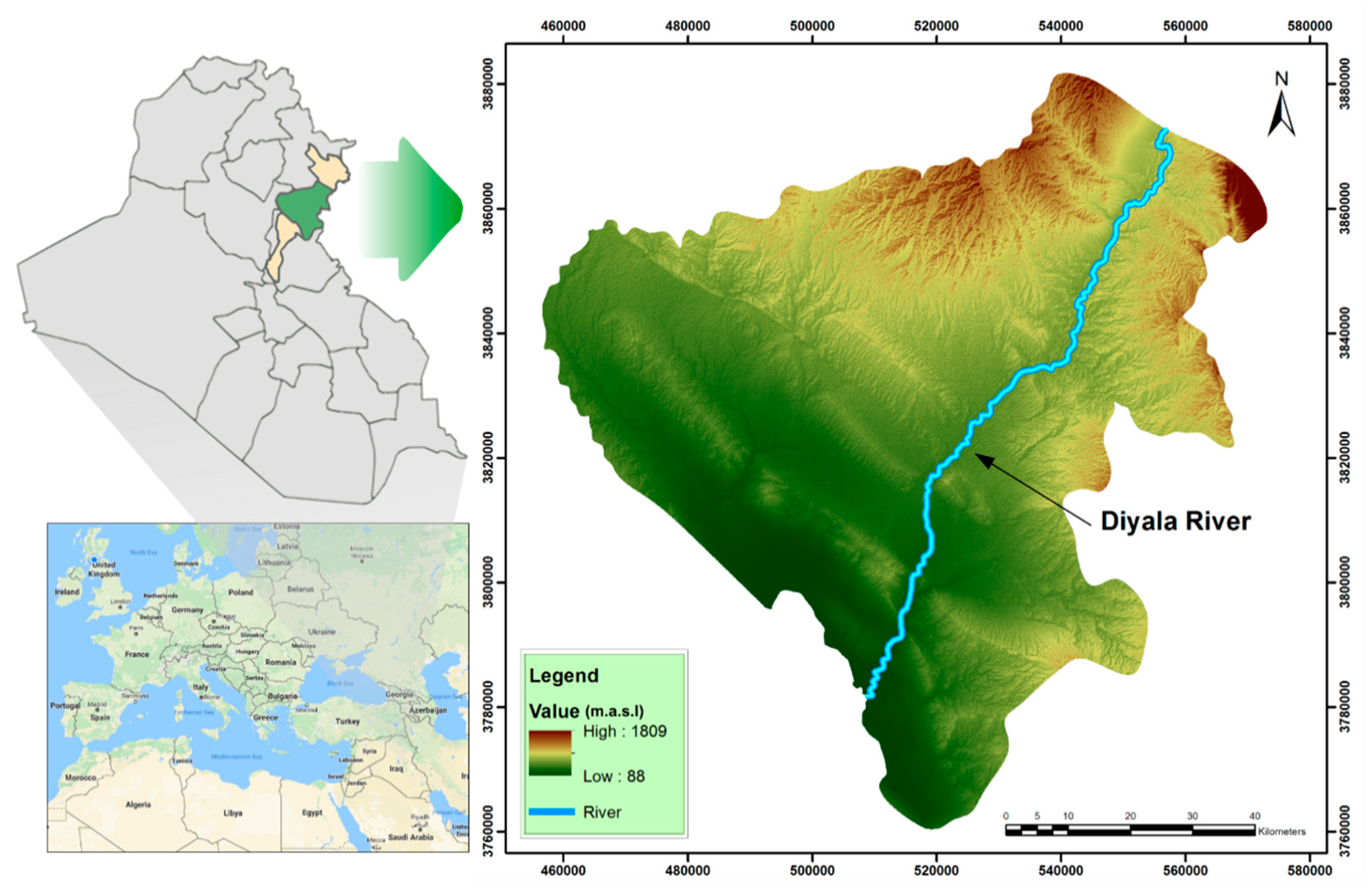
2.1. Case Study Identification

The case study area is located between longitude E 44°30′–45°48′ and Latitude N 33°57′–34°58′ in the northeast of Iraq (Figure 1). It comprises the central part of the Dyiala river basin within Iraq. It is bounded by two multipurpose dams; Derbindikhan located in the north, and Himren in the south, and covers an area of about 7360 km². The land surface elevation ranges between 1809 and 88 m.a.s.l. The average annual rainfall and mean temperature (T_mean) are 285 mm and 24 °C, respectively [29].

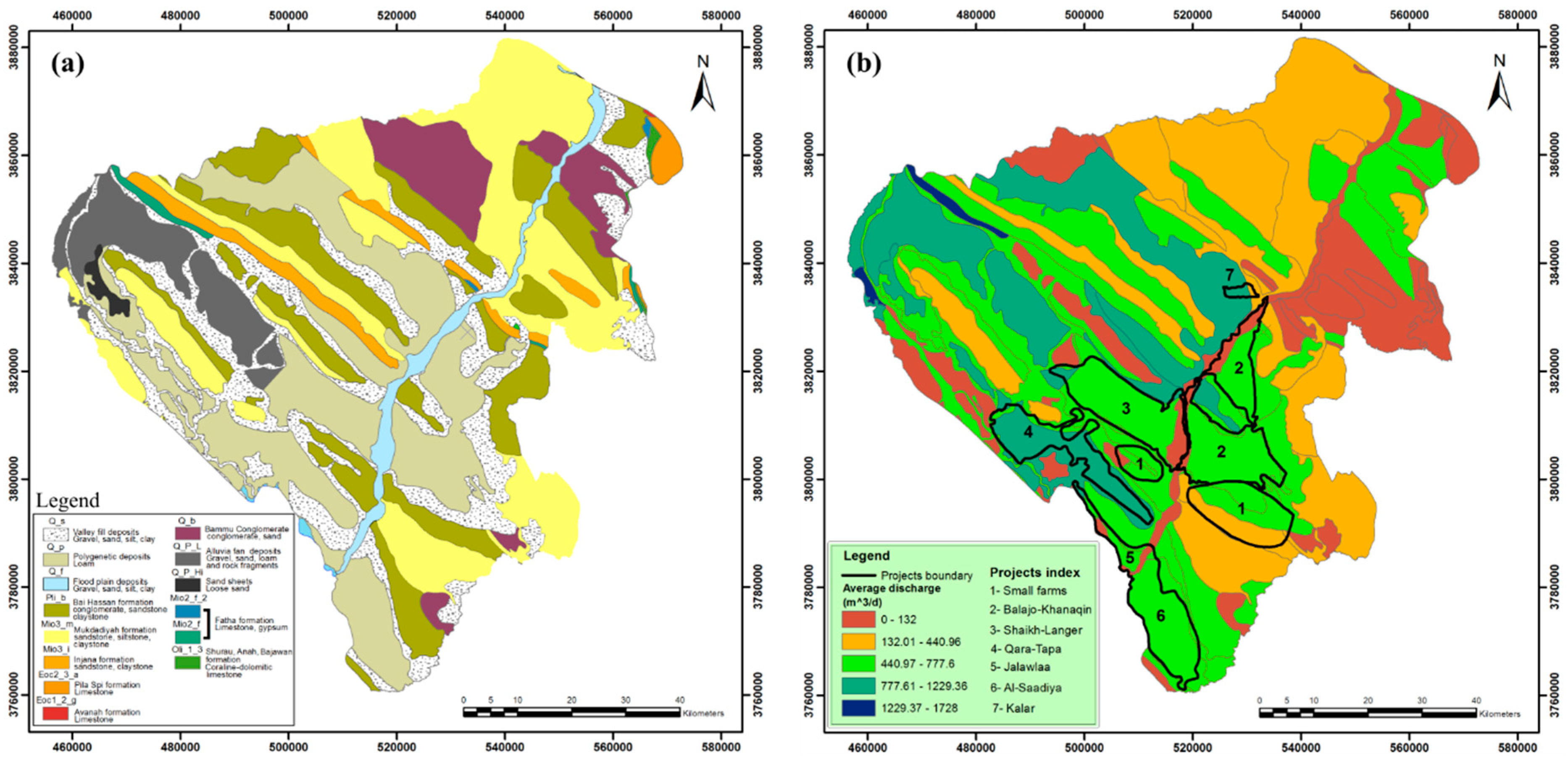
The area is located on a low-angle folded zone, which extends from the northeast foothill areas of Iraq [30]. The tertiary sediments present in a range between middle–late Eocene, represented by Gercus formation, to late Pliocene represented by Bai-Hassan formation. The Quaternary sediments are of late Pliocene–Pleistocene age manifested by Bammu Conglomerate, ending with Valley fill deposit of the Holocene. The stratification is illustrated in Figure 2a.

Groundwater generally flows from the north to the south of the basin, following the topographic surface elevation decline (Figure 1). The main units of hydrogeological significance with aquifer resource potential are the Mukdadiya, Bai-Hassan, and Quaternary deposits. The Quaternary deposits cover a wide portion of the study area with a thickness from 5 to 25 m. It is composed mainly of gravel, sand, and rock fragment. The Bai-Hassan and Mukdadiya formations are considered to be the two major aquifer of this region. The Bai-Hassan formation outcrops at different locations in the study area, while Mukdadiya appears at other parts of the area (Figure 2a). The Mukdadiya formation is composed of fine upward cycles of gravely sandstone, sandstone, and mudstone, while Bai-Hassan is composed of conglomerates with beds of mudstone, siltstone, and sandstone. Their thickness range from 500 to 1000 m [30]. These layers overlay the Injana formation, which is composed mainly of sandstone and claystone. The average hydraulic conductivity for both upper aquifers is 4.88 m/day [29]. Groundwater quality, as characterized by salinity, varies; the total dissolved salts (TDS) ranged between 182 and 5500 mg/L for the upper aquifer (with c. 1000 mg/L being the brackish taste threshold). The estimated aquifer water storage is about 9 × 10⁹ m³, with storage coefficients for the upper and lower aquifer estimated at 3.5% and 0.14%, respectively [31]. The central part of Diyala river basin has many cities, villages, and farms. Since the 1980s, about 1800 wells were drilled [29] in the area due to urban and rural development and associated regional water exploitation increase. Moreover, the government intends to develop and invest in six irrigation projects covering a total area of 647.4 × 10⁶ m² [29,32]. The average aquifer pumping discharge ($Q_{Av}$) within projects areas is about 778 m³/day, which is calculated using spatial analysis in ArcGIS 10.2 depending on the wells’ discharges available in the historical database [29] (Figure 2b).

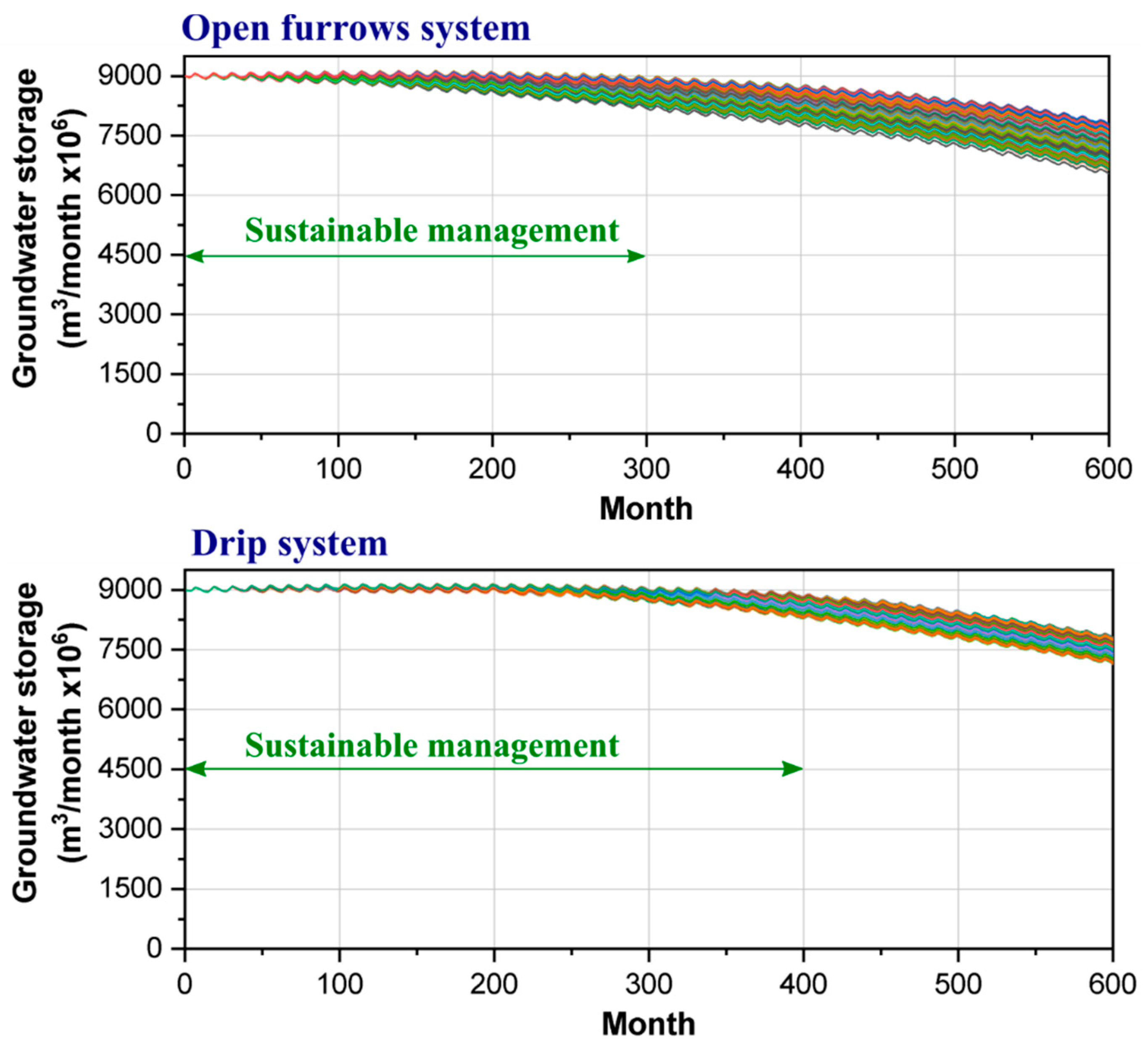
The annual design crop plan pattern exploits 100% of the arable land for winter crops, and 20% for summer crops. The winter crops mainly include wheat, barley, grains, legumes, and berseem, while the summer crops include cotton, rice, sesame and sunflower, vegetables, and cucurbits. The project’s water demands are based upon open furrow irrigation with an efficiency of 65%; hence, 35% loss of the delivered water due to evaporation, on-farm allocation, and infiltration losses. Sprinkler techniques have consistently high evaporative water losses due to the semi-arid environment [32]. Hence, drip irrigation was proposed in this study as an alternative technique to reduce water allocation losses. This has a normal irrigation efficiency of about 90%, and an efficiency of 85% was modelled as a conservative estimate. The total agricultural project’s annual water demand is 567 × 10⁶ m³ [29,32]. This is set within the context of 30 years of meteorological data (precipitation and evapotranspiration) 1981–2010 presented in

Table 1. Average monthly meteorological data (mm) 1981–2010 within the central part of Diayal river basin [29].

Month	Rainfall P	Surface Runoff RO	Reference Evapo-Transpiration ETo	Total Water Balance P-RO-ETo
October	14	0.98	131	−117.98
November	37	2.59	67	−32.59
December	46	3.22	38	4.78
January	61	4.27	36	20.73
February	44	3.08	48	−7.08
March	41.5	2.905	84	−45.41
April	33	2.31	122	−91.31
May	8	0.56	183	−175.56
June	0.5	0.035	229	−228.54
July	0	0	253	−253
August	0	0	234	−234
September	0	0	176	−176
Annual	285	19.95	1600	−1334.95

[29]. The maximum field capacity, according to [33] in [31], is 115 mm, with the surface runoff being equal to 7% of the direct rainfall [34]. The expected future gross total agricultural economic benefit is 160 million USD per year. Hence, the decision makers will require robust water resource management strategies to enable economic benefits to be realized without jeopardizing the sustainability of the water resource.

2.2. Identification of Groundwater Flow Model

The three-dimensional groundwater flow through an aquifer can be expressed by the following finite-difference equation as in [35]

$$\frac{\partial }{\partial x}\left(K_{xx}\frac{\partial h}{\partial x}\right)+\frac{\partial }{\partial y}\left(K_{yy}\frac{\partial h}{\partial y}\right)+\frac{\partial }{\partial z}\left(K_{zz}\frac{\partial h}{\partial z}\right)\pm W=S_S\frac{\partial h}{\partial t}$$

(1)

where K_xx, K_yy, and K_zz are the hydraulic conductivities of the media in x, y, and z direction, respectively. W is a source or sink of water, S_s is the specific storage of the aquifer, h and t represent the groundwater level and time, respectively. Harbaugh and McDonald (1996) present MODFLOW-96 package as a groundwater model solver for steady and unsteady flow. An updated version of MODFLOW-2005 was presented by Harbaugh [36].

Generally, there are two sources of groundwater recharge, which maintain the water for an unconfined aquifer system. The first source is local recharge from rainfall or irrigation water that infiltrate through the soil texture, and the second is from the boundaries of the system: Exchange with neighboring aquifers and water bodies like river, lake, or even sea.

Groundwater recharge at any time t (DP_t) occurs due to the infiltration of access water precipitation (P_t) or irrigation water (IR_t), when soil moisture (SM_t) and the crop evapotranspiration (ET_t) requirements are fully satisfied. The general soil–water balance equation to calculate the infiltrating amount of water to groundwater in the time period t + 1 can be expressed as:

$$S{M}_{t+1}=S{M}_t+P_t+I{R}_t-E{T}_t-R{O}_t-D{P}_t$$

(2)

where $S{M}_{t+1}$ is the soil moisture content at time t + 1; and RO_t is the surface runoff at time t. Deep percolation occurs when the moisture content in soil exceeds the maximum field capacity (maxSM) of the soil, which is defined by Allen et al. [37] as “the amount of water that a well-drained soil should hold against gravitational forces”. Hence, the deep percolation, in case of $S{M}_{t+1}$ > maxSM, can be found as follows

$$D{P}_t=S{M}_{t+1}-maxSM.$$

(3)

The natural aquifer boundary recharges can be calculated using Darcy’s law, as follows:

$$Q=K.I.A_{Sec}$$

(4)

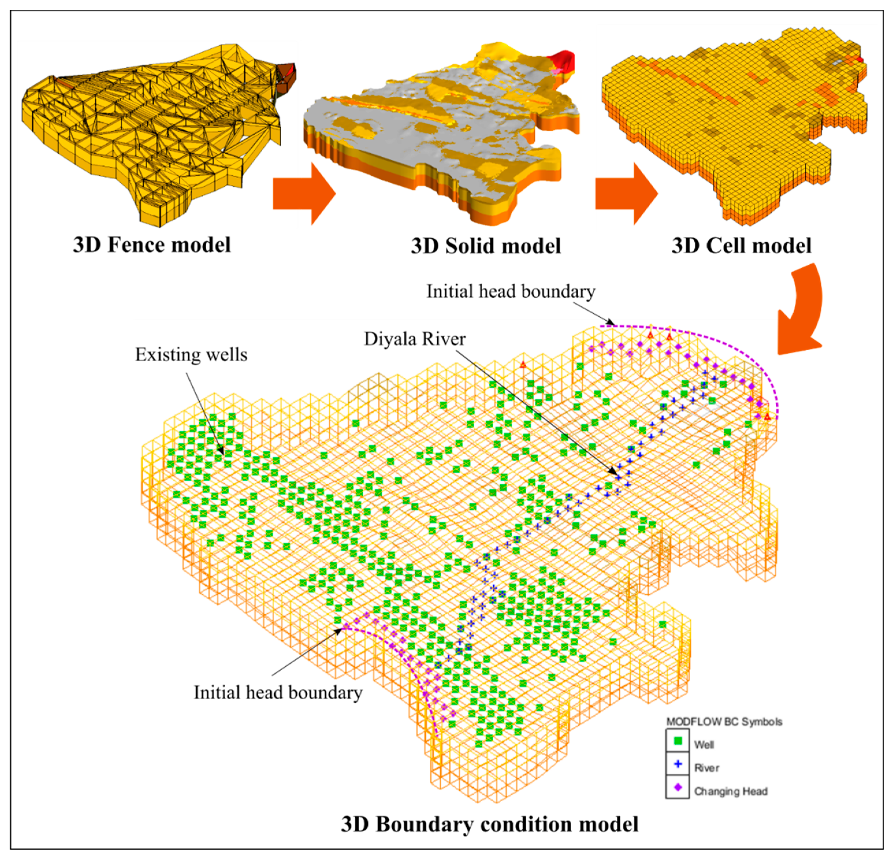
where Q is the groundwater recharge across a boundary section area A_Sec, the aquifer permeability K is the aquifer hydraulic conductivity, and I is the hydraulic (groundwater) gradient where I = ∆h⁄∆l, with ∆h being the difference between the water table head at the recharge and discharge zones of the specified aquifer, and ∆l is the separation distance. These parameters can be calculated using MODFLOW-2005 and GIS techniques. A regional groundwater model had not previously been developed and, hence, a complete regional 3D MODFLOW-2005 model was built for recharge estimation, as in Figure 3. The initial boundary head levels and wells parameters were extracted from wells log database and maps available in SGI et al. [29]. 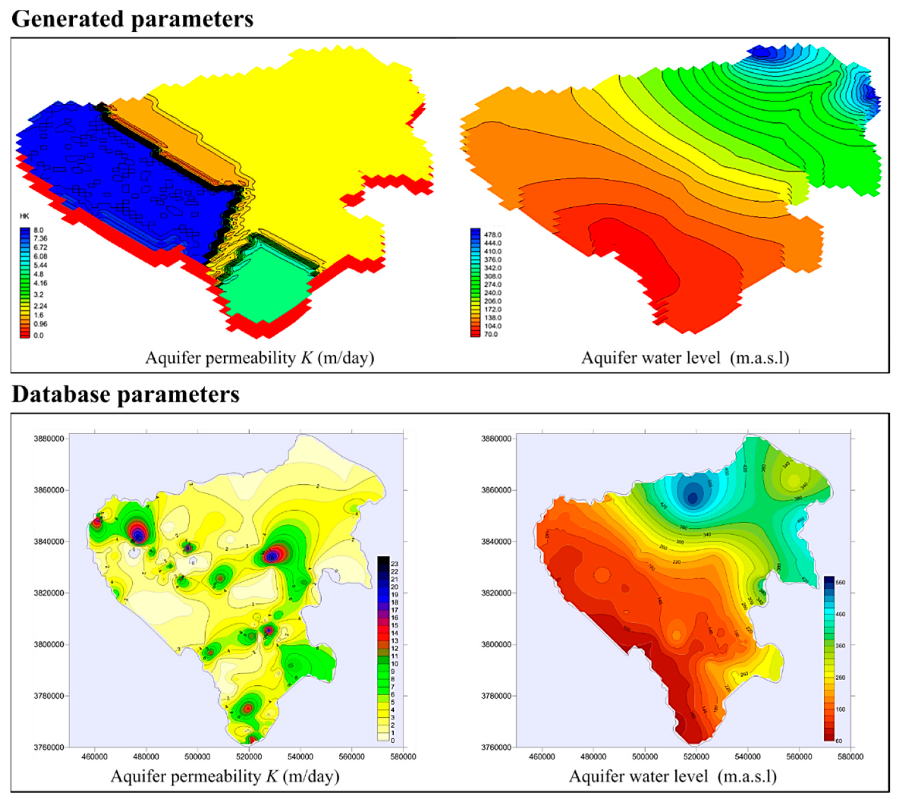The regional water balance in Table 1 shows scarcity in water recharges from the rainfall due to high evapotranspiration rates (ET_o > P), hence zero recharge from rainfall was considered for the simulation model [38]. The simulation model achieved static flow for parameter calibration. The model consists of four layers’ the first two layers are Bai-Hassan and Mukdadiya formation since the two formations are composed of course sediments and are hydraulically connected. The last two layers represent the Injana aquifer system, which is composed of alternation of clay and sand beds. The average thickness of the two systems is 2000 m. The average calibrated K value is about 2.67 m/day and 0.01 m/day for the upper and lower aquifers (Figure 4), respectively, while the upper aquifer boundary recharge TR₀ is about 4.88 × 106 m³/month.

It is obvious from Figure 4 that Diyala River drains groundwater from the northern part of the basin, with that condition reversing gradually to the south. The relation between the groundwater and surface water depends on the riverbed sediments and the water level. In the upper part of the basin, the river is bounded between high-level lands (Figure 1) with coarse bed sediment. This condition changes gradually toward the lower part of the basin, in which the riverbed is higher than the groundwater level with finer bed sediment [39].

Figure 4 also shows the reported aquifer parameters. Cluster and bias in aquifer’s parameters (K) are observed due to irregular distribution of wells across the basin. Here, the aquifer’s water level was presented as a general guide, as they are relevant to wells drilled sequentially over the last 25 years.

2.3. Regional Management Model Identification

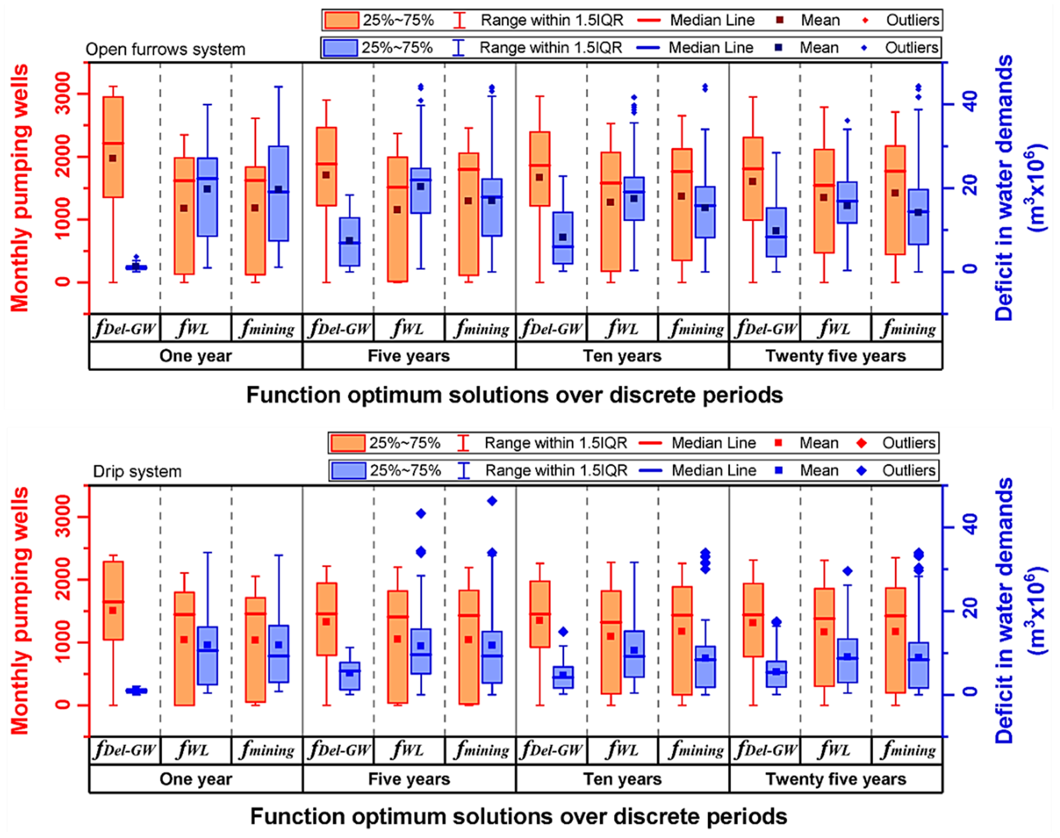
The regional water management strategy aims to fulfil future water demands with sustainable groundwater exploitation; hence, aquifer storage, mining, and infiltration losses should also be considered. Accordingly, decision variables, objectives, and constraints were developed for the optimization approach. Here, the decision variables for the current conceptual model are the numbers of monthly pumping wells (Nw_t) to fulfil the project’s monthly water demands over the proposed operation period.

Table 2. Alternative irrigation methods and operation periods.

Methods of Irrigation	Operation Periods (Months)
Open furrows irrigation (scenario-1)	12	60	120	300	600
Drip irrigation (scenario-2)	12	60	120	300	600

shows the adopted scenarios and operation periods of the model.

To evaluate management strategies for competing groundwater demands in the study area, the first objective is minimizing water deficit between projects’ water demands (PD_t) and the total groundwater withdrawal (G_t) at time t with respect to the project’s maximum demands (PD_max) over the entire considered period (T), which can be expressed by the following formula:

$$min f_{Del-GW}={\displaystyle \sum }_{t=1}^T{\left(\frac{P{D}_t-G_t}{P{D}_{max}}\right)}^2+C^2$$

(5)

$$G_t=N{w}_t\times Q_{av}, N{w}_t=1, 2, \dots N{w}_{max}, N{w}_t\in {\mathbb{N}}^{+}$$

(6)

where Nw_max is the design maximum wells’ number, and C is a penalty factor that includes all models violations, which can be formulated as [40,41]:

$$C=A.{\displaystyle \sum }_{\mathrm{i}=1}^{NC}{g}_i; A\ge 1$$

(7)

where A is a coefficient, NC is the number of constraint violation functions, and $g_i$ represents constraint violations functions; their formula details are presented in Equations (13)–(16).

Usually A is found empirically, which depends on several replications of trial and error [40,41]. This value should be selected carefully to preserve suitable selection pressure to accelerate the algorithm convergence to the near-optimum solutions [42]. Here, a value of A = 10⁴ was selected to exploit all feasible solutions and avoid rendering infeasible solutions at the constraint threshold, especially those with small violation values.

Regional future projection for rainfall was achieved by Abbas et al. [26] using the SWAT model (soil and water associated tool) and GCM (general circulation model) to predict climate changes impacts for a half-century for the entire basin. The average annual rainfall reduction at the end of the half-century was 21%, hence the monthly reduction will be 0.035%. The monthly aquifer rainfall at time t (P_t) can be estimated as:

$$P_t=P\times \left(1-\left(0.035\%\right)\times t\right), t=1, 2,\dots , T.$$

(8)

The second objective is minimizing infiltration losses due to water allocation at time t (DP_t) with respect to maximum soil field capacity (maxSM) over the considered period of time (T), which can be expressed as:

$$min{f}_{WL}={{\displaystyle \sum }}_{t=1}^T{\left(\frac{D{P}_t}{maxSM}\right)}^2+C^2.$$

(9)

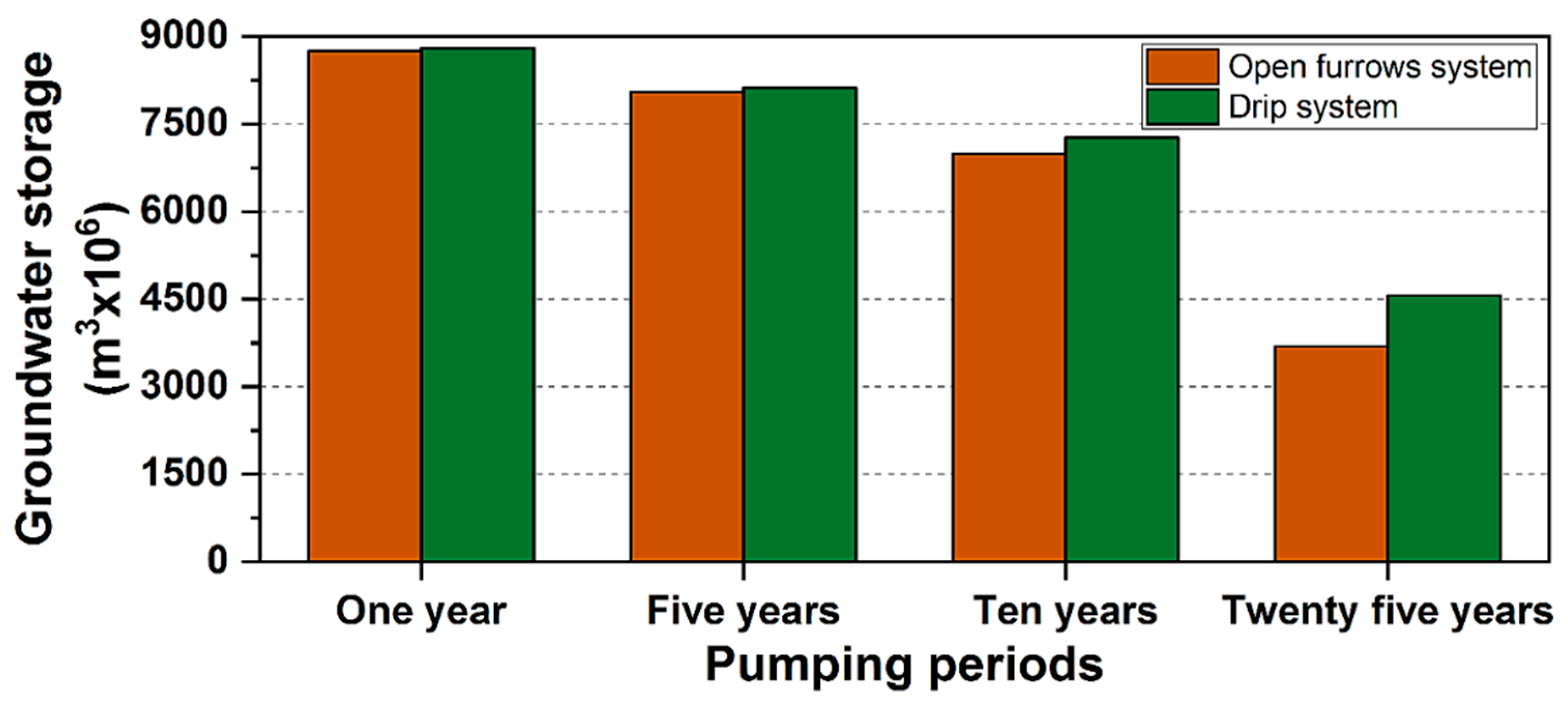
Finally, minimizing the mining from static groundwater storage (S_st) in the aquifers during the extracting process at time t can be expressed as:

$$min{f}_{mining}={\displaystyle \sum }_{t=1}^T{\left(\frac{S_{st}}{S_{aq,t}}\right)}^2+C^2$$

(10)

where S_aq is the aquifer storage calculated from the water balance equation as:

$$S_{aq,t+1}=S_{aq,t}+T{R}_t-G_t$$

(11)

where TR_t is the total water recharges to the aquifers at time t.

Abbas et al. [26] also estimates the average annual groundwater recharge depletion after a half-century for the entire basin about 35%, hence the monthly recharge reduction will be 0.058%. The monthly aquifer boundary recharge at time t (TR_t) can be estimated as:

$$T{R}_t=T{R}_0\times \left(1-\left(0.058\%\right)\times t\right), t=1, 2,\dots , T.$$

(12)

The groundwater management model has multiple operational and environmental constraints, illustrated in

Table 3. Groundwater management constraints in the central part of Diyala river basin.

Parameter	Limitations
Pumping discharge (m3/month × 106)	$0<G_t\le 74.27$ (open furrow) $0<G_t\le 56.79$ (Drip)
Number of wells (per month)	$1\le N{w}_t\le 3183.0$
Soil moisture content (mm/month)	$57.5\le S{M}_t\le 115.0$

. The monthly groundwater pumping discharge (G_t) is equal or less than the project’s maximum water demands, while the monthly number of operated wells (Nw_t) should not exceed the maximum design number (Nw_max). Also, the monthly soil moisture content (SM_t) should be greater than 50% of the maximum soil moisture content (maxSM) to avoid reaching wilting point, in which the plant will die, nor the value of (maxSM) to avoid water deep percolation.

From the above, the constraints functions ${\mathrm{g}}_{\mathrm{i}}$ can be expressed as:

$$g_1={\displaystyle \sum }_{t=1}^{T}Max\left[0, \left(D_t-G_t\right)\right]$$

(13)

$$g_2={\displaystyle \sum }_{t=1}^{T}Max\left[0, \left(N{w}_{max}-N{w}_t\right)\right]$$

(14)

$$g_3={\displaystyle \sum }_{t=1}^{T}Max\left[0, \left(S{M}_t-0.5\times maxSM\right)\right]$$

(15)

$$g_4={{\displaystyle \sum }}_{t=1}^{T}Max\left[0, \left(maxSM-S{M}_t\right)\right].$$

(16)

2.4. MOEA Method Identification

The multi-objectives evolutionary algorithm (MOEA) was used to solve the optimization problem to minimize F(x) = (f1(x), …, fm(x))^T; subjected to: x ∈ Ω, Ω is the decision space and x ∈ Ω is a decision vector. F(x) consists of m objective functions f_i: Ω → R^m, i = 1, …, m where R^m is the objective space.

The multi-objective optimization problem needs a strategy to compare and select solutions, because there is more than one optimum solution in the decision variables space that dominates. Stadler [43] define the Pareto-optimal dominance relation concepts, which is widely used to describe the dominance solutions [44,45]. In a minimization problem, a vector u = (u₁, …, u_m)^T is said to dominate another vector v = (v₁, …, v_m)^T if u_i ≤ v_i for i = 1, …, m and u ≠ v. This can be defined as u ≺ v. Also, a feasible solution x ∈ Ω is called a Pareto-optimal solution; if there is no alternative solution y ∈ Ω such that F(y) ≺ F(x), then the Pareto-optimal set, PS, is the union of all Pareto-optimal solutions, and may be defined as: PS = {x ∈ Ω:∄y ∈ Ω, F(y) ≺ F(x)}. The Pareto-optimal front (PF) is the set comprising the Pareto-optimal solutions in the objective space in a multi-objective optimization problem and is expressed as: PF = {F(x)|x ∈ PS}.

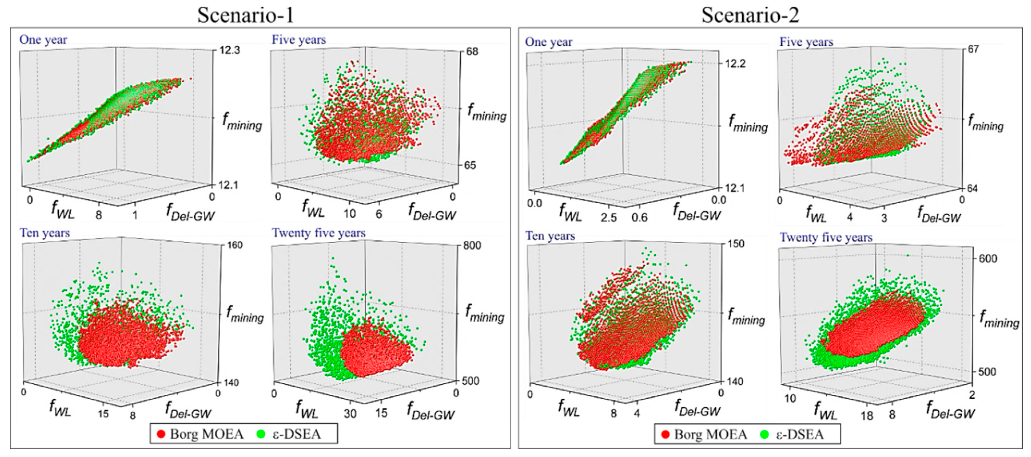
Here, two competitive EAs were adopted to solve the multi-objective problem, Borg MOEA [27] and ε-DSEA [28]. Borg MOEA has many novel concepts to produce optimum solutions and overcome high-dimension complexity. It has a dominance archive to maintain the non-dominated solutions to preserve diversity and convergence. The search space is divided into hyper-boxes, with dimensions equal to ε, and represents the search resolution. The algorithm has an improvement indicator for stagnation monitoring (ε-progress), which monitors the solutions in the dominance archive periodically to check stagnation on local optima. Hence, the algorithm adopts a restart mechanism to revive the search. It has multi recombination operators to generate new solutions and adapt with the one who generates non-dominated solutions in the dominance archive. A competitive assessment of Borg MOEA compared with other state-of-the-art evolutionary algorithms was utilized using multi-objectives problems, through which it outperformed or met these algorithms [27,46,47,48,49].

ε-DSEA has a novel methodology to improve the diversity and the convergence to an optimal solution. The diversity enhanced by implementing multiple operators produces new offspring after an initial random seeding of population. Also, it has a novel methodology to control parameters tuning over the evaluation process for the operators, through which operators’ parameters connected with its performances to produce dominance solutions in the dominance archive. These parameters adjust dynamically within a specified ranged depending on the number of dominance solutions produced by each operator [50,51].

Details of algorithms techniques are in the aforementioned references. The algorithms’ computational parameters are illustrated in

Table 4. Parameter values used in the optimization algorithms.

Parameters	Borg	ε-DSEA 1	Parameters	Borg	ε-DSEA
Initial population size	100	100	SPX parents	10	3
Tournament selection size	2	2	SPX offspring	2	2
SBX crossover rate	1.0	1.0	SPX expansion rate λ	3	[2.5, 3.5]
SBX distribution index η	15.0	[0, 100]	UNDX parents	10	10
DE crossover rate CR	0.1	[0.1, 1.0]	UNDX offspring	2	2
DE step size F	0.5	[0.5, 1.0]	UNDX σζ	0.5	[0.4, 0.6]
PCX parents	10	10	UNDX ση	0.35/$\sqrt{L}$	[0.1, 0.35]/$\sqrt{L}$
PCX offspring	2	2	UM mutation rate	1/L	1/L
PCX ση	0.1	[0.1, 0.3]	PM mutation rate	1/L	1/L
PCX σζ	0.1	[0.1, 0.3]	PM distribution index ηm	20	20

L is the number of decision variables. The permissible range for dynamic parameters is shown in brackets. The parameters σ_η and σ_ζ are standard deviation control the distribution of decision variables. ¹ The initial values of dynamic parameters used in ε-DSEA are as shown for Borg MOEA.

.

A program was written in C language representing Equations (2)–(16). Ten runs were executed for each case, using each of the two scenarios; hence, the total runs were 200 for the entire scenarios and periods, using a desktop PC with Ubuntu 16.04 OS (Core i7-6700 CPU @ 3.4 GHz, 16 GB RAM). The ε values, which is the hyper-box dimension and represent the resolution of the objective function search space, ranged between 0.001 and 0.5 for Equations (5), 0.01 to 0.5 for Equation (9), and from 0.001 to 0.1 for Equation (10). The number of function evaluations ranged between 0.5 × 10⁶ to 1.2 × 10⁶ in both scenarios.

3. Result

3.1. Performance Analysis

To deliver a robust decision management tool to decision makers, an in-depth comparative analysis was reviewed for the selected algorithms. The summary of the best median achievement considered alternatives is presented in

Table 5. Median summary of the best achievement for both algorithms under two irrigation alternative scenarios. The superior results are in bold (smallest values for minimum and largest values for maximum).

Objective	Borg MOEA				ε-DSEA
	12 1	60	120	300	12	60	120	300
	Scenario-1
Min. fDel-GW	0.005	0.916	2.952	10.183	0.006	1.057	2.490	7.988
Max. fDel-GW	1.192	5.362	7.599	15.988	1.244	6.248	9.371	18.922
Min. fWL	0.274	2.05	6.387	19.934	0.161	1.476	4.329	12.839
Max. fWL	7.547	11.606	18.121	34.877	7.426	10.758	18.420	37.521
Min. fmining	12.145	65.077	143.648	544.399	12.142	65.05	143.169	528.478
Max. fmining	12.257	67.656	153.438	649.679	12.256	67.973	158.254	765.451
	Scenario-2
Min. fDel-GW	0.002	0.348	0.889	3.241	0.003	0.436	0.729	2.453
Max. fDel-GW	0.528	3.668	3.997	6.837	0.531	3.159	4.040	8.063
Min. fWL	0.149	1.067	3.758	12.311	0.146	1.074	3.430	9.864
Max. fWL	2.066	4.481	8.079	16.522	2.149	4.006	8.053	17.027
Min. fmining	12.121	64.599	141.408	516.02	12.120	64.607	141.288	506.564
Max. fmining	12.200	66.233	148.191	571.196	12.200	66.730	149.655	601.931

¹ Number of months.

, and the complete achievements are highlighted in bold. Detail results are available in the Supplementary Materials. Both algorithms develop competitive optimum solutions, but in most alternatives, ε-DSEA achieved better results. Note that excessive groundwater mining of the estimated aquifer storage (9.0 × 10⁹ m³) was predicted after 40 years of water exploitation, hence the 50-year alternative (600 months) is not presented here.

The median range solutions selected to illustrate the Pareto-front optimality achieved by both algorithms for the adopted scenarios, as shown in Figure 5 Comparable results were achieved by both, however ε-DSEA has wider Pareto-fronts especially when decision variables evolve (e.g., 120 and 300 for the 10- and 25-year alternatives, respectively) in both scenarios, which have the advantage of the solutions’ diversity. As a result, decision management strategies as predicted by ε-DSEA were selected for review.

3.2. Groundwater Optimum Management

Figure 6 presents a monthly summary of operating wells (the decision variables) and the deficit in water farms delivery for both scenarios. The average optimum number of wells used in an open furrow system ranged 1100–2000 for one year of pumping compared to 1300–1600 (variable used). However, if investment included drip irrigation systems, the number of pumping wells declined to 1000–1500 for one year of pumping and 1000–1300 for variable pumping scenarios. Furthermore, the median number of extraction wells was 1400 when using the drip system for all periods, while the range was from 1500 to 1850 using open furrow irrigation. Generally, the drip system results show less deficit in water delivery to the farms. The average value for the drip system was 15 × 10⁶ m³/month, and it ranged from 15 × 10⁶ to 20 × 10⁶ m³/month for the open furrows system.

The effect of water exploitation on groundwater storage is illustrated in Figure 7, and shows the lowest storage achieved for different pumping periods for both water delivery alternatives. Groundwater storage depletion is obvious for medium- and long-term pumping, while drip irrigation reduces the impact on aquifer storage. For one-year pumping, the depletion was 4%, while for 5- and 10-year pumping, it was about 12% and 25%, respectively, for both irrigation system alternatives. The final storage depletions were 61% and 55% for open furrows and drip system, for 25-year pumping, respectively. All alternatives show unsustainability in groundwater storage management due to scarcity in the aquifers’ water recharge, as shown in

Table 6. Summary of pumping discharges and aquifer recharges for the optimum solution achieved by each objective function over considered periods using open furrows and drip irrigation system (m³/month × 10⁶).

Operating Periods (Years)	${\mathit{f}}_{\mathit{D}\mathit{e}\mathit{l}-\mathit{G}\mathit{W}}$	${\mathit{f}}_{\mathit{W}\mathit{L}}$	${\mathit{f}}_{\mathit{m}\mathit{i}\mathit{n}\mathit{i}\mathit{n}\mathit{g}}$	${\mathit{f}}_{\mathit{D}\mathit{e}\mathit{l}-\mathit{G}\mathit{W}}$	${\mathit{f}}_{\mathit{W}\mathit{L}}$	${\mathit{f}}_{\mathit{m}\mathit{i}\mathit{n}\mathit{i}\mathit{n}\mathit{g}}$
	Mean			Median
	Pumping discharge—Scenario-1
One	45.95	27.48	27.56	51.67	37.78	37.96
Five	39.81	26.93	30.24	44.00	35.44	42.00
Ten	38.97	29.75	31.94	43.51	36.87	41.15
Twenty-five	37.43	31.44	33.06	42.22	35.99	41.32
	groundwater recharge—Scenario-1
One	18.31	3.34	3.99	16.46	0.00	0.00
Five	18.20	5.42	11.62	8.08	0.00	2.11
Ten	17.91	7.60	13.26	7.78	0.00	2.46
Twenty-five	16.15	8.79	14.06	7.79	1.17	3.88
	Pumping discharge—Scenario-2
One	35.12	24.24	24.20	38.45	33.73	33.95
Five	30.94	24.46	24.28	34.02	32.89	33.40
Ten	31.49	25.56	27.39	33.88	30.79	33.46
Twenty-five	30.61	27.11	27.26	33.63	32.23	33.24
	groundwater recharge—Scenario-2
One	11.63	3.14	3.32	6.80	0.00	0.00
Five	11.36	4.21	6.79	5.02	0.00	0.00
Ten	11.91	5.85	9.80	5.11	0.00	1.23
Twenty-five	10.88	7.81	9.24	5.04	0.99	1.43

f_Del-GW, f_WL, and f_mining refer to groundwater delivery, water losses, and mining objectives functions, respectively.

.

The results show significant differences between the groundwater exploitation and aquifer recharge over the adopted pumping scenarios. The depletion in recharges ranged between 50% to 80% for mean values, and between 60% to 100% for the median values, in comparison with the pumping discharges.

The results show unsustainable regional groundwater resource for all alternative plans due to high water demands and the aquifers’ recharge scarcity in this semi-arid environment. Hence, other alternatives are needed to reduce water demands by either reducing the areas irrigated or changing to less water-demanding crop types. A sustainable groundwater management resource budget is forward modelled for the next half-century considering these. Sustainability may be achieved when the projects’ water demands are reduced by 45% as a minimum for both irrigation alternatives (Figure 8). The use of open furrows maintains aquifer storage for about 25 years compared to the drip system of about 33 years. The average final storage depletions in both alternatives is 22% and 16%, respectively. Hence, using a drip irrigation system in this region should be considered beneficial and may represent a more sustainable groundwater management practice.

4. Discussion

4.1. Model Performance

The use of predictive optimization model results depends on the confidence of the results as used by decision makers. Here, model performance analysis demonstrates the merit of ε-DSEA techniques to generate optimum solutions. Both algorithms have six recombination operations (for EA evolution process); the Borg technique tended to adapt a single operator, while ε-DSEA adapted with two. Figure 9 illustrates the auto-adapted and the self-adaptive mechanism for Borg MOEA and ε-DSEA in all alternatives. Borg MOEA adapted with PCX recombination operator in all periods in both scenarios. This phenomenon was also observed and discussed before [52], in which the new offspring generated in the vicinity and around the selected parents may cause the stagnation of the algorithm.

Conversely, ε-DSEA is adapted with both PCX and SPX operators in parallel to generate optimum solutions. The resetting methodology in ε-DSEA succeeds in changing the operators’ adaptation to escape from local optimam which remains clear in all operation periods. In Scenario-1, the ε-DSEA was initially adapted with SBX operator during the first year of operation, then adapted with PCX and SPX operators after the first resetting was triggered (revive process).

For Scenario-2, ε-DSEA adapted with SBX operators for one and five years, and with PCX and SPX operators for 10 and 25 years. This shows the robustness of the ε-DSEA methodologies to adapt rapidly with different environment problems and escape from local optima.

4.2. Groundwater Management Results

The robust results achieved by ε-DSEA shows regional storage shortfalls after 40 years of water exploitation, even with the use of drip irrigation, due to scarcity of aquifer recharge. However, possible sustainable management plans may be achieved for the next half-century by reducing aquifer stresses. The decision makers (the Iraqi’s government) should consider a future policy to reduce projects’ water demands in this region. New legislation should set out to control unauthorized drilling and pumping to reduce regional water exploitation. Other alternatives are required, including conjunctive use with surface water, aquifer storage and recovery (ASR) initiatives, as well as the rehabilitation of leaky water conveyance infrastructure. In addition, there is a lack of information of trans-boundary (in Iran) aquifer exploitation for the considered trans-boundary basin, which may have direct effects on aquifer recharge (subsurface and deep aquifers recharge). Hence, modelling should extend to cover these regions by developing data exchange collaboration with the trans-boundary country for better representative and management.

The results provide a prediction of future groundwater management alternatives for decision makers to consider within future policies for strategic sustainable water resources management for the investigated study area with potential for wider implementation in other regions with comparable scenarios. Optimization algorithms and the available dataset were successfully employed as an alternative to highly expensive simulation and field investigations to highlight the relevant driving parameters of water crisis in the region. The model could be developed to consider more management objectives, including surface water, towards integrated water resources management.

5. Conclusions

This research showed that, in the study area, aquifer stresses due to investment planning, growth, and the water–food–energy nexus coupled with climate change impact are inevitable. Two optimization algorithms were employed to develop and deliver options for a groundwater sustainable management strategy. The optimization problem was formulated for long-term farm irrigation with three objective function for five discrete periods with up to 600 decision variables using two water delivery alternatives for agriculture. The study utilized a developed and calibrated groundwater simulation model built in MODFLOW-2005 GMS software (groundwater modelling system by Aquveo LLC, Utah, USA). Both algorithms executed 10 random seedings for each alternative, leading to the ε-DSEA providing more robust results when compared to the Borg MOEA for almost all alternatives; hence, the relevant results were adopted. This endorses the use of multiple optimization algorithms to select the most competitive results, since algorithms’ optimality achievement vary under different problem environments [2]. The results for the Diyala Basin demonstrate that groundwater storage depletion was 25% over 10 years of water exploitation, increasing to about 60% over 25 years. The aquifer storage was completely exhausted after 40 years in both alternatives due to low aquifer recharge caused by low rainfall and high evapotranspiration rates (semi-arid zone). The introduction of drip irrigation mitigates the impact on the aquifer storage over the discrete periods, especially for long-term water exploitation. The probability of sustainable groundwater resource management was scenario modelled for the next half-century by reducing water delivery demands. The results show that a possible sustainable storage budget using an open furrows system can be achieved for the next 25 years, and 33 years for a drip system with 45% demand’s yield for both. Hence, the decision makers should consider future policy to reduce water demands by either changing crops types or reducing farms areas. Also, the use of a drip system for water allocation should be considered in policy since it has less impacts on groundwater yields. Conjunctive use with surface water may also be considered, to mitigate groundwater depletion and maintain its sustainability.