Article

Evapotranspiration from Horizontal Subsurface Flow Constructed Wetlands Planted with Different Perennial Plant Species

1
Department of Agricultural, Food and Environment (Di3A), University of Catania, Via S. Sofia 100, 95123 Catania, Italy
2
Centre for the Conservation and Management of Nature and Agroecosystems (CUTGANA), University of Catania, Via S. Sofia 100, 95123 Catania, Italy
3
Department of Agricultural and Food Sciences (DISTAL), University of Bologna, Viale Giuseppe Fanin 50, 20147 Bologna, Italy
*
Author to whom correspondence should be addressed.
Water 2019, 11(10), 2159; https://doi.org/10.3390/w11102159
Submission received: 11 September 2019 / Revised: 11 October 2019 / Accepted: 14 October 2019 / Published: 17 October 2019

Abstract

:
This paper presents the results of an experiment carried out in Southern Italy (Sicily) on the estimation evapotranspiration (ET) in pilot constructed wetlands planted with different species (Chrysopogon zizanioides, Myscanthus x giganteus, Arundo donax, Phragmites australis, and Cyperus papyrus). In the two monitored growing seasons, reference ET0 was calculated with the Penman-Monteith formula, while actual ET and crop coefficients were measured through a water balance and the FAO 56 approach, respectively. The highest average seasonal ET value was observed in Phragmites australis (17.31 mm d−1) followed by Arundo donax (11.23 mm day−1) Chrysopogon zizanioides (8.56 mm day−1), Cyperus papyrus (7.86 mm day−1), and Myscanthus x giganteus (7.35 mm day−1). For all plants, crop coefficient values showed different patterns in relation to growth stages and were strongly correlated with phenological parameters. Myscanthus x giganteus and Arundo donax showed a water use efficiency values significantly higher than those observed for the other tested species. Results of this study may contribute to select appropriate plant species for constructed wetlands located in semi-arid regions, especially when the use of reclaimed water and/or the use of aboveground biomass are planned.

1. Introduction

Constructed wetlands (CWs) are sustainable and efficient solutions used around the world to treat wastewater as an alternative or a supplement to intensively engineered treatment plants. CWs are complex, integrated systems involving water, plants, animals, microorganisms, and the environment. They are used to improve the quality of point and nonpoint sources of water pollution, including municipal wastewater, urban stormwater, agricultural run-off, industrial wastewater, landfill leachate, and mine drainage [1], in which wastewater reuse also plays a crucial role [2].
The plant growing phases in CWs have several characteristics in relation to the treatment process, which make plants an indispensable component of the design. In fact, they provide a surface for the microbial biofilm growth and also stabilize the bed with their dense root systems, improve the hydraulic conditions of wastewater flow through the medium, reduce the water’s current velocities, isolate the surface bed against frost in winter, release oxygen from roots into the rhizosphere, and uptake pollutants from treated wastewater [3].
Another important aspect is their role in water loss via evapotranspiration (ET) from the CW systems. Many wetland plants are not able to store water, as most terrestrial plants do, and consequently they transfer substantial amounts of water to the atmosphere, especially under warm and windy conditions. In these conditions the ET of wetland plants may be seven to eight times higher than the evaporation without plants. This has been shown in other studies [4,5] conducted in eastern Sicily (Italy), where the ET of Phragmites australis in a pilot horizontal sub surface flow (H-SSF) system reached up to about 50 mm day−1. El Hamouri et al. [6] found evapotranspiration rates of about 57 mm day−1 in reed bed systems in Morocco. These high evapotranspiration rates clearly reduce the wastewater volumetric flow through the CW, leading to an increase in hydraulic retention time and concentrations of non-degradable contaminants in the effluent. On the other hand, longer retention times improved treatment performance for degradable contaminants due to the increase in time for microbial activities [7], the sedimentation of suspended solids and insoluble particles [8], and plant uptake [9].
The ET estimation is particularly important for the systems, such as sludge treatment wetlands, where it represents a key element for their efficiency and successful long-term functioning. Sludge treatment wetlands (STWs), also known as sludge drying reed beds, are widely used in Northern Europe to dewater and mineralize waste sludge and septage from wastewater treatment plants [10]. These systems generally consist of a number of reed beds built as planted vertical filters with an efficient drainage system in order to dewater the sludge effectively. After initial drainage of the free-water from the loaded sludge, ET becomes the main process responsible for further dewatering, removing water held by capillary forces. STWs are primarily vegetated with Phragmites australis however, due to the growing interest in applying this technology in arid and semi-arid regions, is necessary to evaluate other alternative species also according to ET characteristics.
Conversely, in the CWs designed to reuse treated wastewater, the ET process is considered as non-desirable because it reduces the wastewater volume available for reuse and increases salt concentration [11,12]. There is evidence that excess salts originate from the irrigation, while treated wastewater leads to the long-term deterioration of soils [13] and sometimes causes short-term damage to crops [14].
There is thus an urgent need to analyze the ET values of the different plant species used in CWs under various climatic conditions. Some studies were carried out on the ET of Phragmites australis [5,15,16,17,18], because it is the main species used in CWs, while very few data are available on the ET capacity of other macrophytes [19,20,21,22,23]. ET rates could be easily estimated by the FAO 56 approach [24], multiplying the reference ET (ET0), calculated with the Penman-Monteith equation using local meteorological data, by the crop coefficient (Kc). However, there is a lack of information and data on Kc for the various wetland plants [12,22,25,26]. Finally, another parameter for selecting plants for CWs could be the aboveground biomass productivity, e.g., for energy purposes. Again, there is very little information in the literature on CW biomass productivity [27,28,29,30].
Consequently, the main aim of this study was to conduct a comparative evaluation of evapotranspiration rates in pilot-scale constructed wetlands planted with different herbaceous species. These species were selected for their potential high biomass yield as a renewable energy source. In this way the CWS could represent a sustainable and integrated system for municipal wastewater management, linked to energy crop production. Plants usually used in CWs (Cyperus papyrus, Chrysopogon zizanioides, Arundo donax, and Phragmites australis) or biomass crop (Miscanthus x giganteus) have been chosen. The two-year study has allowed to determine the ET rates, crop coefficients, aboveground biomass productivity and water use efficiency (WUE) index of five plant species, and investigate the effects of the meteorological conditions and plant growth phase on ET and Kc.
The obtained information is strategic for the CW wastewater reuse perspective.

2. Materials and Methods

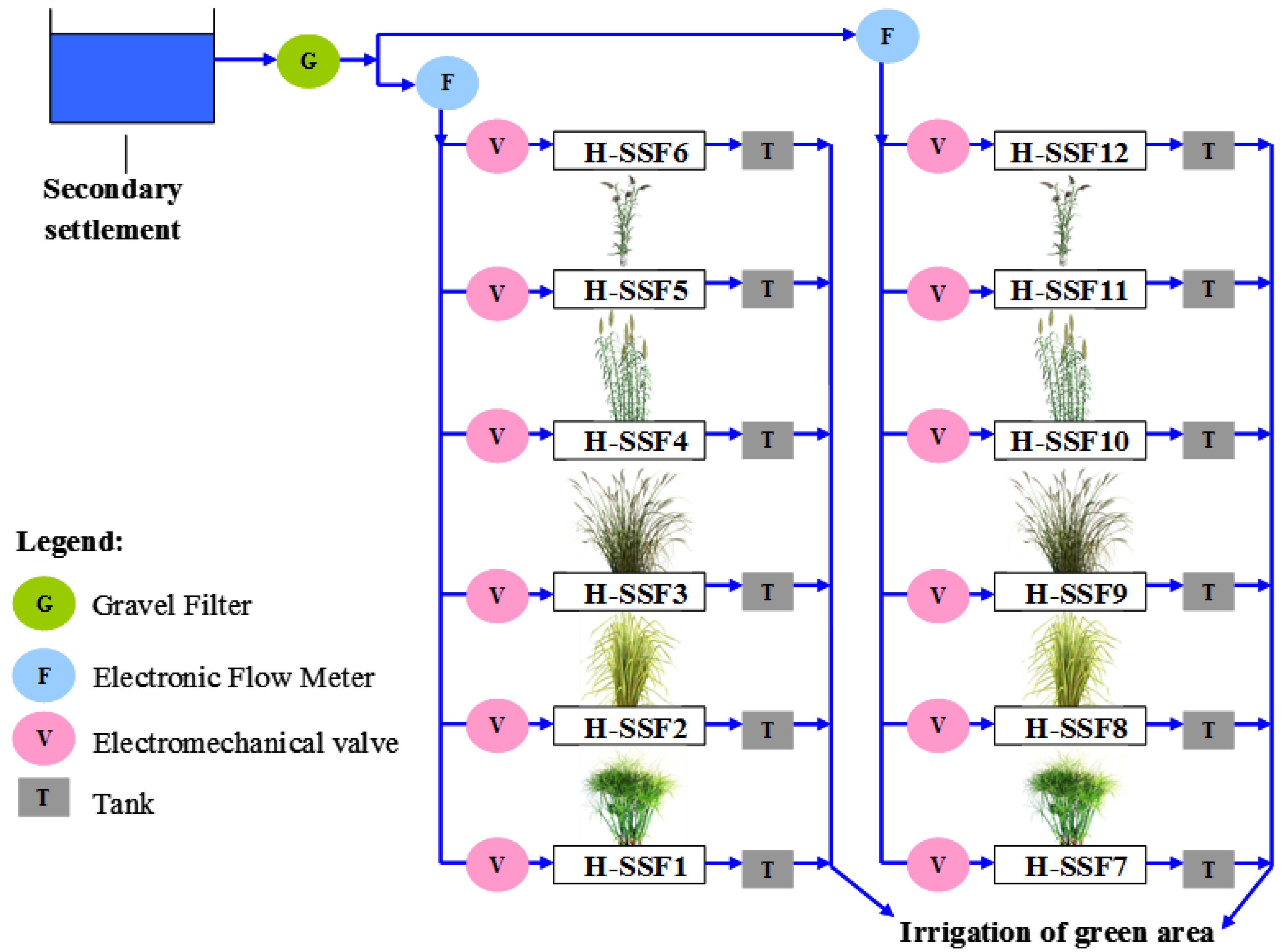
2.1. Experimental Plant Design

The experimental plant is located in San Michele di Ganzaria (latitude 37°30′ N, longitude 14°25′ E, 370 m a.s.l.), a small community (5000 inhabitants) in eastern Sicily, characterized by Mediterranean semiarid climate.
The constructed wetland pilot plants (CWPPs) were used for tertiary treatment of a portion of the effluent from the municipal wastewater treatment plant (WWTP). This involved a pre-treatment step followed by an Imhoff tank, a trickling filter, and secondary settlement. The CWPP was made up of two lines, each one consisting of six H-SSF constructed wetlands functioning in parallel (Figure 1).
Wastewater from the effluent of the secondary clarifier first passed through a filter, to prevent the wastewater distribution pipes from clogging, and was then diverted to the two lines.
From April to December 2012 and 2013, the monitoring of physical and chemical characteristics of CWPP influent was carried out (Table 1). A total of 18 samples (nine in 2012 and seven in 2013) were collected and analyzed by standard methods [31]. In 2013 the mean influent pollutant concentrations were generally higher than the values observed in 2012, with lower standard deviations.
In the H-SSF CW beds, the influent is distributed at the bed-head through a perforated 16 mm PEBD pipe transversal to the flow direction to facilitate uniform wastewater distribution into the bed. Wastewater in the terminal section was intercepted by a transversal perforated pipe connected to an adjustable outlet (spiral plastic pipe) to control the water level in the filtering bed. Wastewater effluent from each bed, was first collected in a plastic tank (one per bed), where a submersible pump with a water level sensor was located for intermittent emptying of the tank, which was then used for the irrigation of a green area close to the pilot plant.
In each line, five beds were planted with different herbaceous species, while one bed was unvegetated (control). Cyperus papyrus (L.) was planted in H-SSF1 and H-SSF7, Chrysopogon zizanioides (L.) Nash in H-SSF2 and H-SSF8, Miscanthus x giganteus Greef et Deu. in H-SSF3 and H-SSF9, and Arundo donax (L.) in H-SSF4 and H-SSF10, Phragmites australis (Cav.) Trin. in H-SSF5 and H-SSF11, while H-SSF6 and H-SSF12 were left unplanted. All these herbaceous plants were planted in November 2011, except for C. papyrus which was planted later (June 2012), with a density of about six plants/m2. In all vegetated beds, the plant cover was fully developed in August 2012. In the CW beds planted with C. papyrus, the experimental activity was carried out only in the first year (2012).
Each bed was 1.5 m wide, 3.0 m long, and 0.8 m deep, built with concrete and waterproofed with an impermeable liner. The beds were filled to 0.6 m, with volcanic gravel (10–15 mm). A piezometer was placed at the outlet of each bed to monitor the water level.

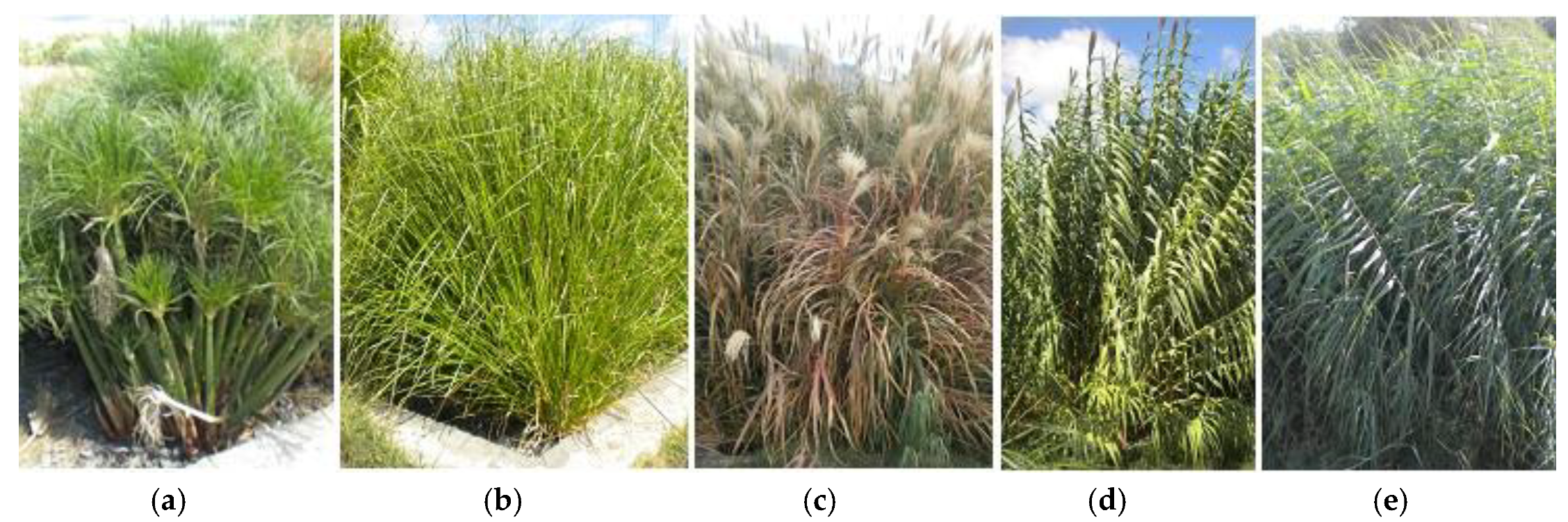
2.2. Herbaceous Plants

In this work plant species belonging to Poaceae (A. donax, M. giganteus, P. australis, and C. zizanioides) and Cyperaceae (C. papyrus) families were investigated (Figure 2); they have different carbon fixation mechanisms and C3 and C4 photosynthetic cycles.
Arundo donax L. is a C3 grass which is widespread in the riparian areas of the Mediterranean and is found over a wide range of the world’s subtropical and warm-temperature areas [32,33,34]. A. donax has been planted for centuries as an erosion controller and roof-thatching material and has also been used as feed and fodder for livestock [35]. In recent years A. donax aroused the interest of the scientific community because if has some characteristics that make it suitable for wastewater treatment in CW [36] and as a new source of biomass for energy production. These characteristics include its rapid growth rate, high biomass productivity, apparent salt tolerance, easy propagation from rhizomes, limited number of pests, and the various potential uses for aboveground biomass.
Miscanthus is a C4 grass originating from East Asia. Miscanthus x giganteus [37] is a natural and sterile hybrid of M. sinensis and M. sacchariflorus [38] which is native to Japan and was introduced vegetatively into Denmark in 1935 for horticultural uses [39]. It has been extensively studied in Europe since the early 1980s as it is considered as one of the most promising biomass crops for non-food use (energy, cellulose pulp, compost, etc.) [39,40,41].
Phragmites australis (Cav.) Trin. Former Steud is a cosmopolitan C3 emergent macrophyte species which is the most preferred plant among ecological engineers for use in constructed wetlands [42]. This is due to its rapid growth, high biomass production, and great capacity for nutrient accumulation [43,44,45].
Chrysopogon zizanioides (L.) Nash is a perennial tropical C4 grass native to India. It has been successfully used for soil and water conservation due to its robust root system and tolerance for adverse environmental conditions [46].
Cyperus papyrus (L.) like other productive tropical emergent wetland species, uses the C4 photosynthetic pathway [47]. It is a rhizomatous perennial plant and is widely distributed in the Nile River Valley of Northern Africa, Madagascar, and Mediterranean countries [48,49,50,51]. It is naturalized in Sicily (Italy) and Florida (USA) [52] and has also extended its distribution into Indonesia, Israel, Syrian Arab Republic, Taiwan, China, and elsewhere.

2.3. Measurement of Bio-Agronomic Characteristics

The bio-agronomical survey and sampling activity were carried out in three 0.5 m2 sampling areas selected at the opposite ends and in the middle of each bed. In each sampling area, bio-agronomical analysis on five random plants was made with the goal of evaluating the basal stem diameter, total leaves, and plant height. Basal stem diameter was measured about 5 cm aboveground with a slide calliper while plant height was measured from the bed surface to the last node (A. donax, M. giganteus, and P. australis), the apex of the central leaf (C. zizanioides) or to the inflorescence (C. papyrus). The plant density was measured on the total area of the sampling areas. During the first growing season (from April to November 2012), the beds were surveyed every 10 days, while in the second season they were surveyed only at the beginning and at the end of the season. At the end of each investigation period, vegetation was harvested from the surface of each sampling area in order to evaluate the aboveground fresh biomass production. In order to evaluate the dry biomass production, the fresh biomass samples were dried in a thermo-ventilated oven at 65 °C until a constant weight.

2.4. Measurement of Evapotranspiration Rates and Crop Coefficients Estimation

Wastewater flow rate treated in the CW (about 50–150 L h−1) was measured by two electronic flow meters, installed at the inlet pipe of each line and connected to a control panel to record the influent wastewater flow rate for each bed. For each bed, this control panel also recorded the effluent discharge volume and regulated the open/closing time of the electromechanical valves, the latter installed in the inlet pipe of each wetland.
Air temperature, wind speed and direction, rainfall, global radiation, and relative humidity were measured by a CR510 automatic weather station (Campbell Scientific, Logan, UT, USA) installed close to the experimental plant.
The influent wastewater flow rate and the effluent wastewater discharge volume, combined with precipitation data measured by the meteorological station were used to estimate the evapotranspiration rates of the plant species during the vegetative periods (from April to November in 2012 and 2013), using a water balance method:
E T = Q i A + P D v A
where ET (mm day−1) is the evapotranspiration of the herbaceous species, Qi is the influent flow rate (mm3 day−1), A is the surface area of the wetland (mm2), P is the net precipitation (mm day−1), and Dv is the discharge volume (mm3 day−1).
Evapotranspiration daily data (ET) were cumulated and averaged over 10-day periods.
The reference ET (ET0 in mm day−1) was calculated with a spreadsheet program, PMday.xls [53,54], using the standardized Penman-Monteith equation [55] and implemented with data taken from an on-site weather station following Borin et al. [4].
The average 10-day crop coefficient was calculated using the FAO-56 crop coefficient approach [24], as:
K c = E T E T 0
where ET is the 10-day measured evapotranspiration (mm) and ET0 is the 10-day reference evapotranspiration (mm).
In order to evaluate the evapotranspiration effect on the treated wastewater salinity the electrical conductivity (EC) was measured by a probe (Delta OHM—HD 2106.2), each two/three weeks, in the CW influent and in the effluent of each bed.

2.5. Evaluation of Water Use Efficiency Indices

The amount of biomass yield produced per unit of used water is referred to as the water use efficiency [56]. It is mainly used in agriculture and can be applied to the water lost in producing the economic or the biological yield. The WUE index could be a useful tool for the selection of plant species used in constructed wetlands if using the aboveground biomass yield (e.g., for energy purposes).
Over the study period, for each herbaceous species, the WUE index (g L−1) was calculated with the following equation:
W U E = Y E T
where Y is the dry biomass yield (g m−2) at the final harvest and ET is the evapotranspiration water (L m−2).

2.6. Statistical Analysis

Statistical analysis of data was performed using Minitab® 16 Statistical Software. The bio-agronomical results were analysed using ANOVA after verifying the homogeneity of the variances using the Bartlett test and the normality of distribution of the recorded data with Shapiro–Wilk test. The Student–Newman-Keuls test was used for means separation (p < 0.05).

3. Results and Discussion

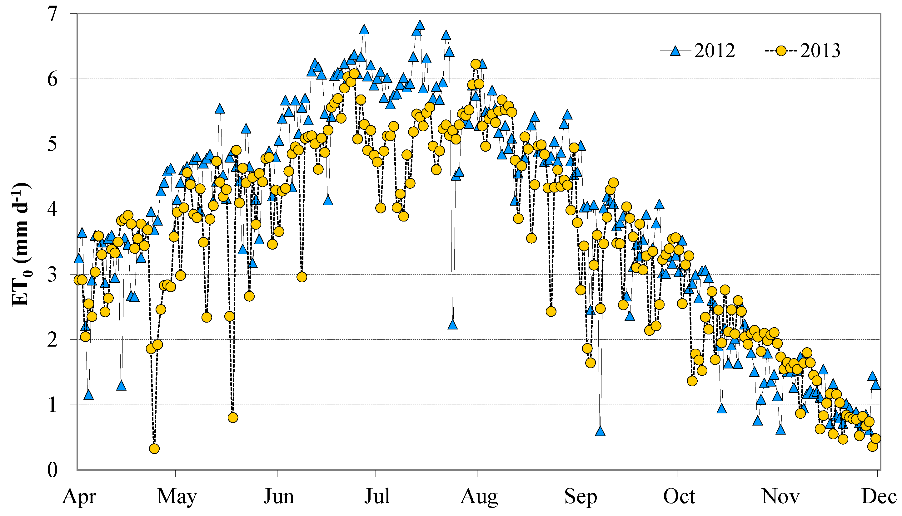
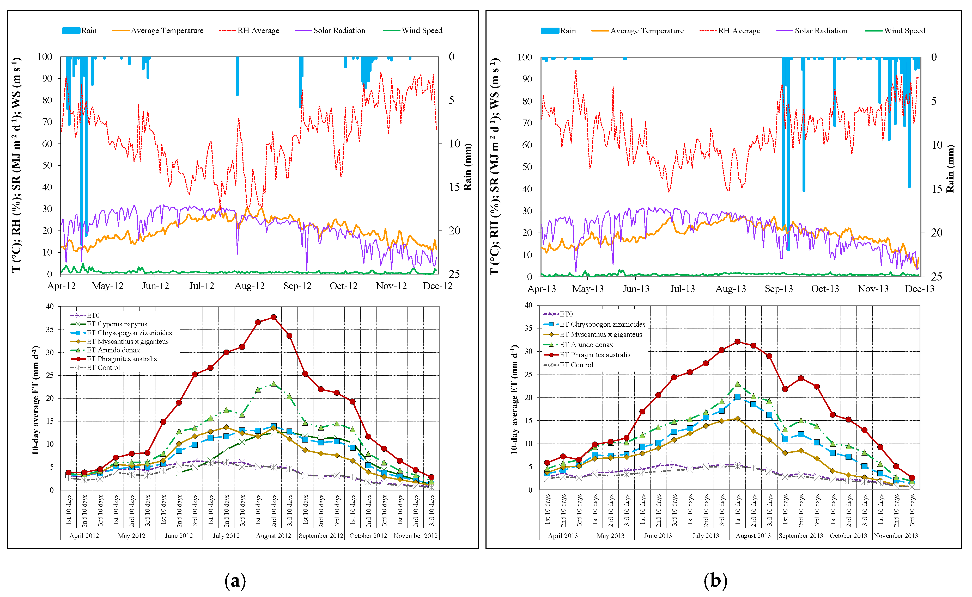
3.1. Meteorological Conditions

The experimental area is characterized by a typical Mediterranean dry climate (long-term average precipitation is around 500 mm year−1), with relatively humid winters, and dry and warm summers. The monthly meteorological data detected during the experimental activity are shown in Table 2. Total rainfall in 2012 and 2013 were drier than the average long-term precipitations, with only 390 mm year−1 in 2012 and 290 mm year−1 in 2013. However, during the 2013 growing season (from April to November), the total precipitation was about 33% higher than in 2012. There was also a different temporal distribution of precipitation within the two growing seasons. In 2012 the rainfall was concentrated in the first half of the growing season, while in 2013, the rainfall was concentrated in the second half of the investigation period.
The two growing seasons were characterized by temperatures that ranged from −1.6 °C (November 2013) to 43.4 °C (July 2014), and an average relative humidity from 47.5% (July 2012) to 83.5% (November 2012). During the first observation period, the average temperature was higher (20.1 °C) than in the second (19.2 °C), while an opposite trend was observed for the average relative humidity (63.1% in 2012 and 65.6% in 2013).
The average seasonal wind speed values were very similar but with different trends: In 2012 the highest values were detected in April and May, while in 2013 the highest values were in August and September.
Similar values were also detected for the seasonal total solar radiation with 5253 and 5196 MJm−2 day−1 in 2012 and 2013, respectively.

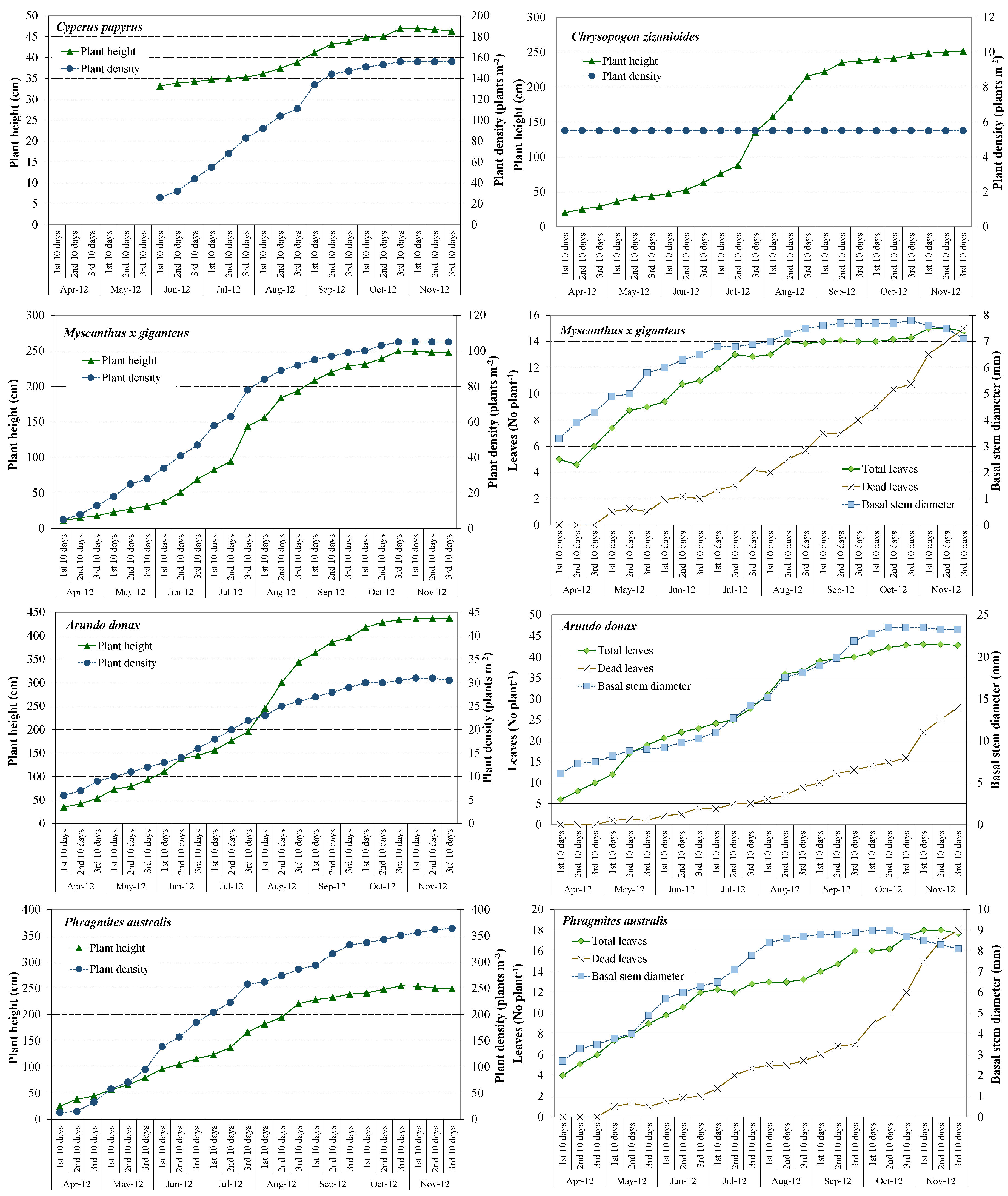
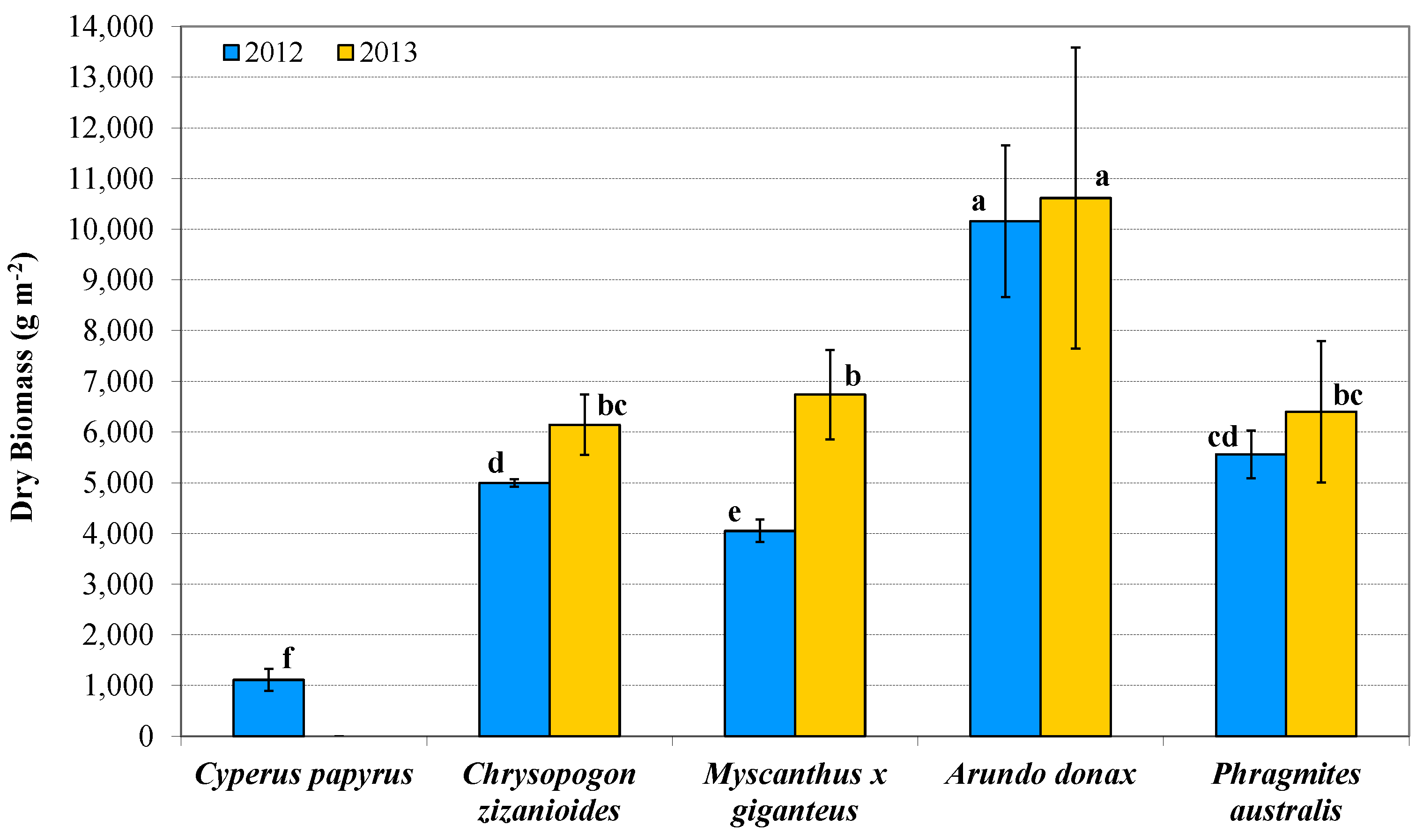
3.2. Plant Development and Biomass Production

As expected, the bio-agronomical analyses highlighted that increasing plant age positively influenced the plant height, basal stem diameter, total leaves, and plant density. For all tested species, except for C. papyrus, the plant heights were significantly different at the beginning and at the end of each investigation period and, consequently, for M. giganteus, A. donax, and P. australis, also the basal stem diameter and total leaves. At the end of the investigation periods, A. donax showed the highest plant height (mean value of about 439 cm) followed by C. zizanioides, M. giganteus, and P. australis, which showed no significantly different heights (mean value of about 258 cm), and then C. papyrus. The plant density increased significantly between the first and the second survey periods, with the biggest increase being for M. giganteus (+37% between the end of the two investigation periods) (Table 3).
The data collected in the first year highlighted a variation in the plant growth rate over the season (Figure 3). For C. zizanioides and M. giganteus, between early April to mid-June the plant growth showed a constant rate (mean about 0.51 cm day−1). These plants showed an increase in height until October with a maximum growth rate detected from mid-July to late August for C. zizanioides (average 3.12 cm day−1) and between mid-July and mid-August for M. giganteus (average 2.89 cm day−1). In November the plant height remained relatively constant. The height of P. australis’ was characterized by an almost constant increase from April to mid-July (average 1.12 cm day−1) and from the end of August to mid-October (average 0.53 cm day−1), by a maximum increase phase (average 2.03 cm day−1) from mid-July to the end of August, and an almost constant phase from mid-October to the end of November. A. donax showed the highest growth rates compared to the other species tested, with a maximum average value, of about 4.78 cm day−1, recorded from the end of July to late August. Conversely, C. papyrus showed the lowest growth rate, just 0.07 cm day−1 for the entire growing season. In 2013, although the same measurements reported in Figure 3 were not performed, the growth rates of the different investigated plant species did not reveal significant changes compared to the previous year.
In terms of plant density, the species showed different trends. For C. zizanioides, as expected, the plant density remained constant throughout the investigation period, while C. papyrus, M. giganteus, and A. donax showed an increased plant density until October. Throughout the first season, P. australis showed an average stem emission value of about 1.43 stem m−2 day−1.
The time pattern of the average total number of leaves per plant was comparable to that of plant height with the highest leaf emission rate highlighted for A. donax (an average of about five leaves per plant per month). The senescence of leaves started in May and stopped, for M. giganteus and P. australis, at the end of the first investigation period with full senescence. While for A. donax, at the end of November 2012 there were still about 15 green leaves per plant. Also, the time pattern of the basal stem diameter was similar to that of the plant height with a first increase up to October, reaching a maximum of 7.8 mm for M. giganteus, 9.0 mm for P. australis, and 23.5 mm for A. donax.
Arundo’s above-ground dry biomass was significantly different from the other species (Figure 4) showing the highest mean value of about 10,385 g m−2. The biomass yield of this species was comparable to that obtained (10,700 g m−2 yr−1) by Idris et al. [36] in a similar CW located in Australia, and by Borin et al. [57] in an open field experiment carried out, under high water and N input, in a Mediterranean environment (maximum yield values 98,000 g m−2 yr−1).
The dry yields of C. zizanioides and M. giganteus produced in the second growing season were significantly higher than those obtained in the first season, due to a significant increase in plant density or plant height. These species together with P. australis, in the second year, showed no significant differences between the dry biomass yield, with an average value of about 6426 g m−2.
The dry yield of P. australis recorded throughout this study was higher than measured in other studies carried out in Europe under temperate climates [29,58,59], but comparable with the values reported in studies conducted in similar climates [5,60].
It was not possible to show comparative above-ground dry biomass productivity for M. giganteus with other CW as no research on this was found. However, several field trials have been carried out on M. giganteus cultivated in open field conditions under different environments, in order to investigate their potential yield. The results highlighted a lower dry yield than our study, ranging from to 1000 to 4900 g m−2 [33,61].
Vetiver’s average dry biomass values ranged between 4992 and 6144 g m−2, which were comparable to those obtained in other similar experiments carried out in CW, which ranged between 4070 and 7920 g m−2 [62,63].
Due to the shorter planting duration, the above-ground biomass of the C. papyrus in this study was significantly lower (up to −90%) than other species tested and to previous studies [64,65]. However, their differences in various sites were attributed to prevailing climatic conditions.

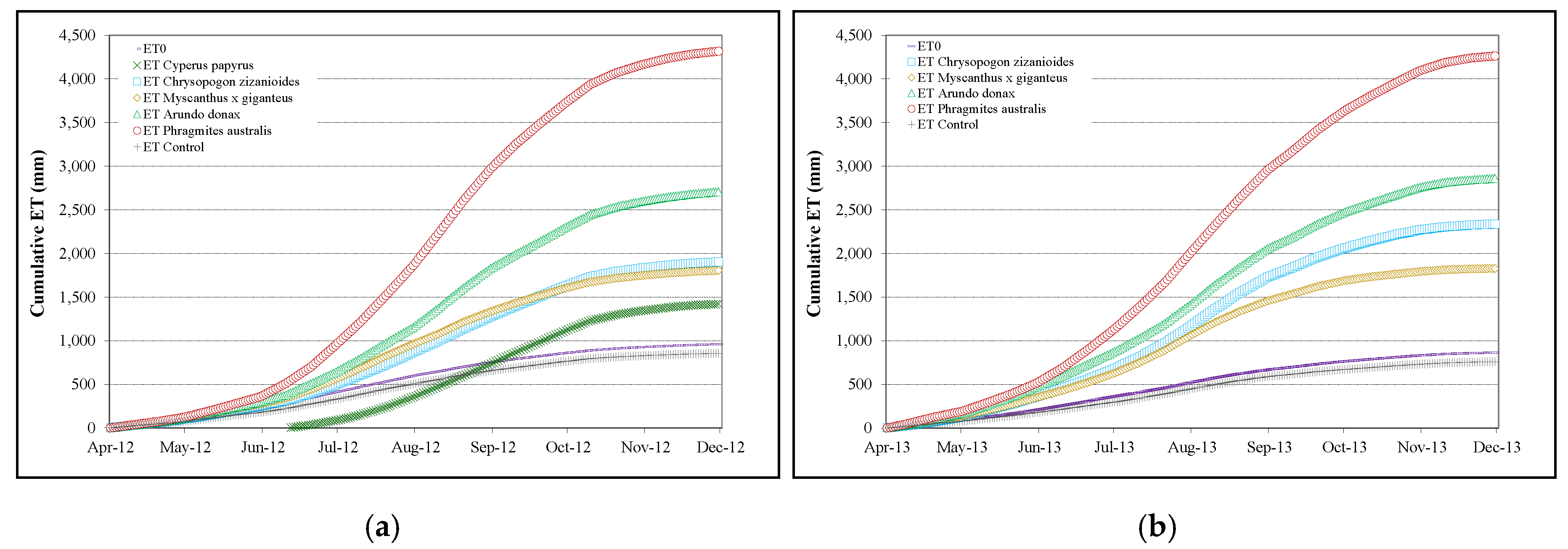
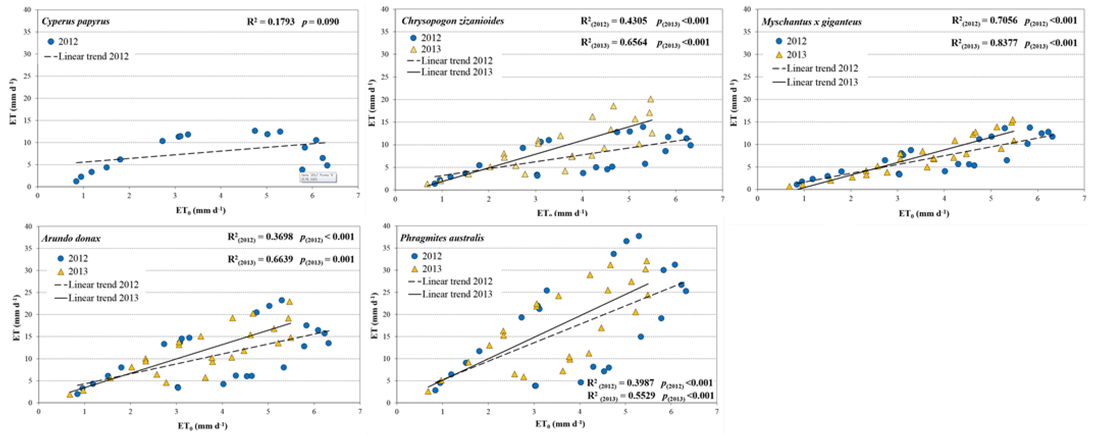
3.3. Evapotranspiration Measurements

During the two investigation periods, daily ET0 trends were similar except from the beginning of June to the end of July (Figure 5) when the 2012 ET0 values (mean value 5.76 mm day−1) were generally higher than in 2013 (mean value 5.07 mm day−1) due to the higher temperature associated with lower relative humidities.
On average, the daily seasonal ET0 was similar in both years: 3.90 mm day−1 and 3.55 mm day−1 in 2012 and 2013, respectively. Daily ET0 values ranged from 0.60 to 6.83 mm day−1 in 2012 and from 0.33 to 6.23 mm day−1 in 2013.
In both years, the lowest average monthly ET0 values were recorded in November (Autumn), 1.10 mm day−1 in 2012 and 1.07 mm day−1 in 2013, and the highest in July (Summer) with 5.74 mm day−1 (2012) and 5.07 mm day−1 (2013).
The 10-day average ETcon presented trends which were very similar to the 10-day average ET0 (Figure 6) with daily ETcon values ranging from 0.60 to 6.19 mm day−1 in 2012 and from 0.65 to 5.12 mm day−1 in 2013. Cumulative ETcon was similar in the two years (856 mm in 2012, and 761 mm in 2013) and about 10% lower than cumulative ET0 (Figure 7).
As expected, marked differences in evapotranspiration rates were observed between planted and unplanted CWPPs. All species showed an increase in 10-day average ET trends with a maximum in August, when the maximum plant growth stages were recorded, followed by a decrease in November due to the progress in plant senescence. Different 10-day average ET trends were highlighted in the vegetated beds in the first two months of each investigation period, with an increase in ET cumulative values from the 2012 to the 2013 season, of about 60% (A. donax), 44% (P. australis and C. zizanioides), and 27% (M. giganteus). This could be explained by the higher vegetative growth occurring at the initial phase of the second season compared to the same period in the first season, as demonstrated by statistically significant differences between the plant density and/or height values. P. australis was found to have a higher average 10-day ET values (ranging from 2.60 to 37.67 mm day−1), followed by A. donax (1.89 ÷ 23.20 mm day−1), C. zizanioides (1.34 ÷ 20.15 mm day−1), M. giganteus (0.63 ÷ 15.46 mm day−1), and C. papyrus (1.23 ÷ 12.62 mm day−1).
As reported in Figure 6, evapotranspiration is strongly influenced by climatic conditions: ET rates decreased in relation to rainfall events. For P. australis and A. donax, which showed no significant differences in dry biomass yield between the two seasons, the higher average 10-day ET values were shown in the second 10 days of August 2012 (37.67 and 23.20 mm day−1 for P. australis and A. donax, respectively) compared to the same period in 2013 (32.13 and 22.99 mm day−1 for P. australis and A. donax, respectively). This was due to the higher air temperature and solar radiation associated with a lower relative humidity detected in August. For M. giganteus and C. zizanioides, the significantly higher dry biomass values in 2013 led to similar or higher ET rates (C. zizanioides) than in 2012, despite the different climatic conditions. In fact, the cumulative ET of M. giganteus and C. zizanioides in 2012 and 2013 was, 1805 and 1904 mm, and 1831 and 2341 mm, respectively. CWPPs vegetated with P. australis showed the highest cumulative ET values (4318 mm in 2012 and 4269 mm in 2013), while the lowest cumulative ET value was detected for C. papyrus (1421 in 2012). However, note that this value is cumulative over six months compared to eight months for the other species.
Over the whole period, the highest average ET value was measured in the CWPPs vegetated with P. australis (17.31 mm day−1). This value is comparable with the average ET value of P. australis (16.87 mm day−1) found by Rozkošný et al. [66] in a CWPP located in Lesonice (Czech Republic). It is also much higher than those obtained in other similar experiments carried out in temperate climates, where the average ET ranged from 0.2 to 7.74 mm day−1 [67,68,69]. In addition, it is lower than that reported by El Hamouri et al. [6], who measured an average annual ET rate of about 57 mm day−1 in horizontal subsurface CW (size 28 m2) in Rabat (Morocco).
In the CW described above also for A. donax, El Hamouri et al. [6] found a much greater average ET (57 mm day−1) than that obtained in our study (11.23 mm day−1). Also, in a HSSF pilot plant (50 m long and 1 m wide) located in Sicily (Italy). Tuttolomondo et al. [12] observed a higher cumulative ET of A. donax (about +50%). Instead in a study carried out in an open field in Tuscany (Italy), the estimated cumulative ET of A. donax was about 60% lower [70].
Regarding the ET of C. papyrus, very few data are available in the literature for a similar experimental plant. Kyambadde et al. [71] reported an ET rate from C. papyrus of 24.5 mm day−1 for a HSSF in Kampala (Uganda), which is about three times higher than that shown in our study.
With regard to C. zizanioides and M. giganteus, no evapotranspiration studies have been conducted in CWs. However, in central Italy, in lysimeter (0.90 m deep, 1.2 m long, and 1.2 m wide), Triana et al. [70] estimated ET cumulative values for M. giganteus of 772 mm and 991 mm (an ET value of only about 26% was found in our study).
The linear trends of average 10-day ET for each species versus average 10-day ET0 were calculated for both years (Figure 8). The trend lines showed that 10-day ET for all species, except C. papyrus, correlated significantly with 10-day ET0 with correlation factors (R2) ranging from 0.370 (A. donax in 2012 season) to 0.838 (M. giganteus showed the highest R2 in both seasons). This is in agreement with other research carried out in Mediterranean environments [5,12,22].
As expected, vegetation species and ET rates have not influenced the EC in the treated wastewater. The average EC value in the CW influent was 1230 µS cm−1, while in the CW effluents was about 1225 µS cm−1 at unplanted units, 1235 at C. papyrus, M. giganteus, and C.zizanoides units, 1248 µS cm−1 at A. donax beds and 1264 µS cm−1 at P. australis beds. However, also in the summer season, when the water loss through ET process reached the highest values (up to 12% of the influent flow rate in P. australis beds), the differences between the EC values detected in treated and untreated wastewater were not significant.

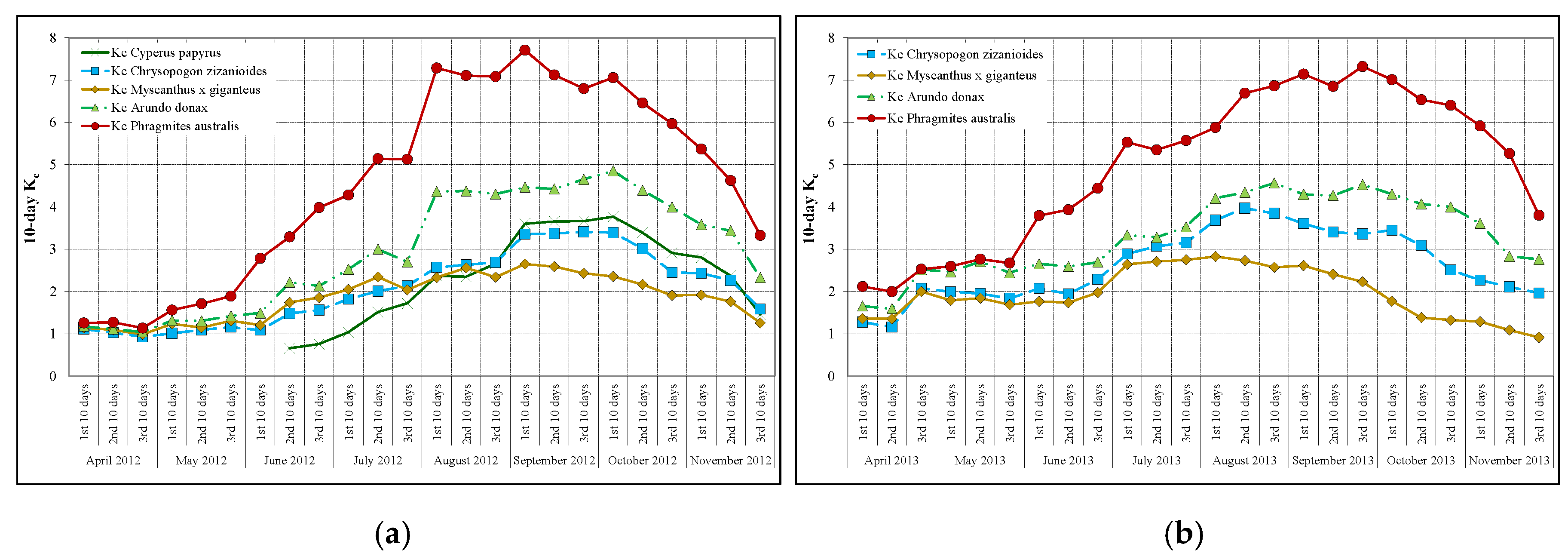
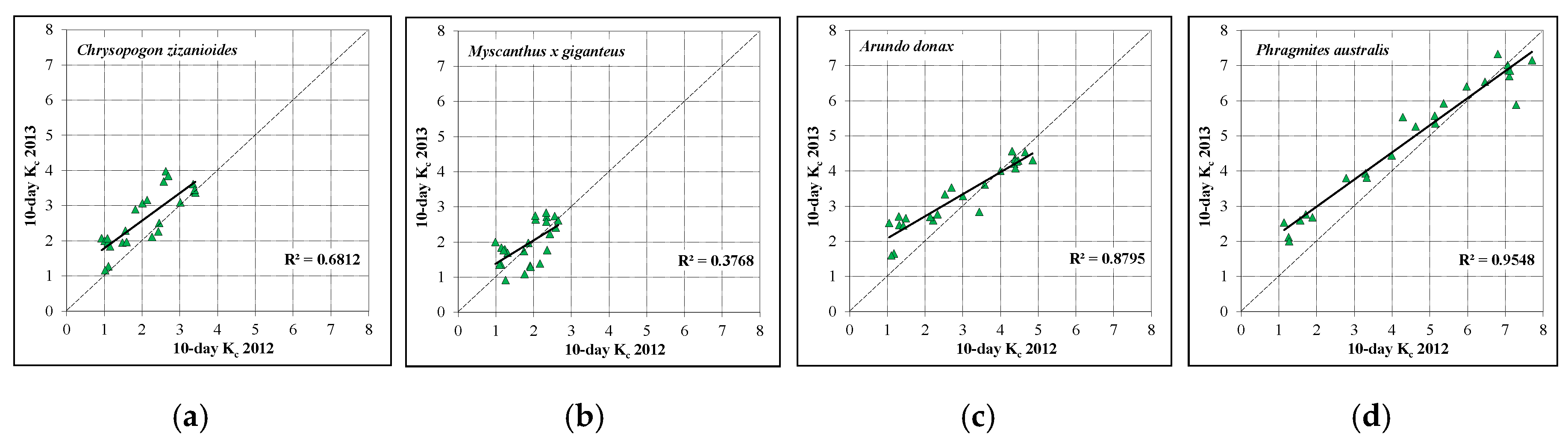
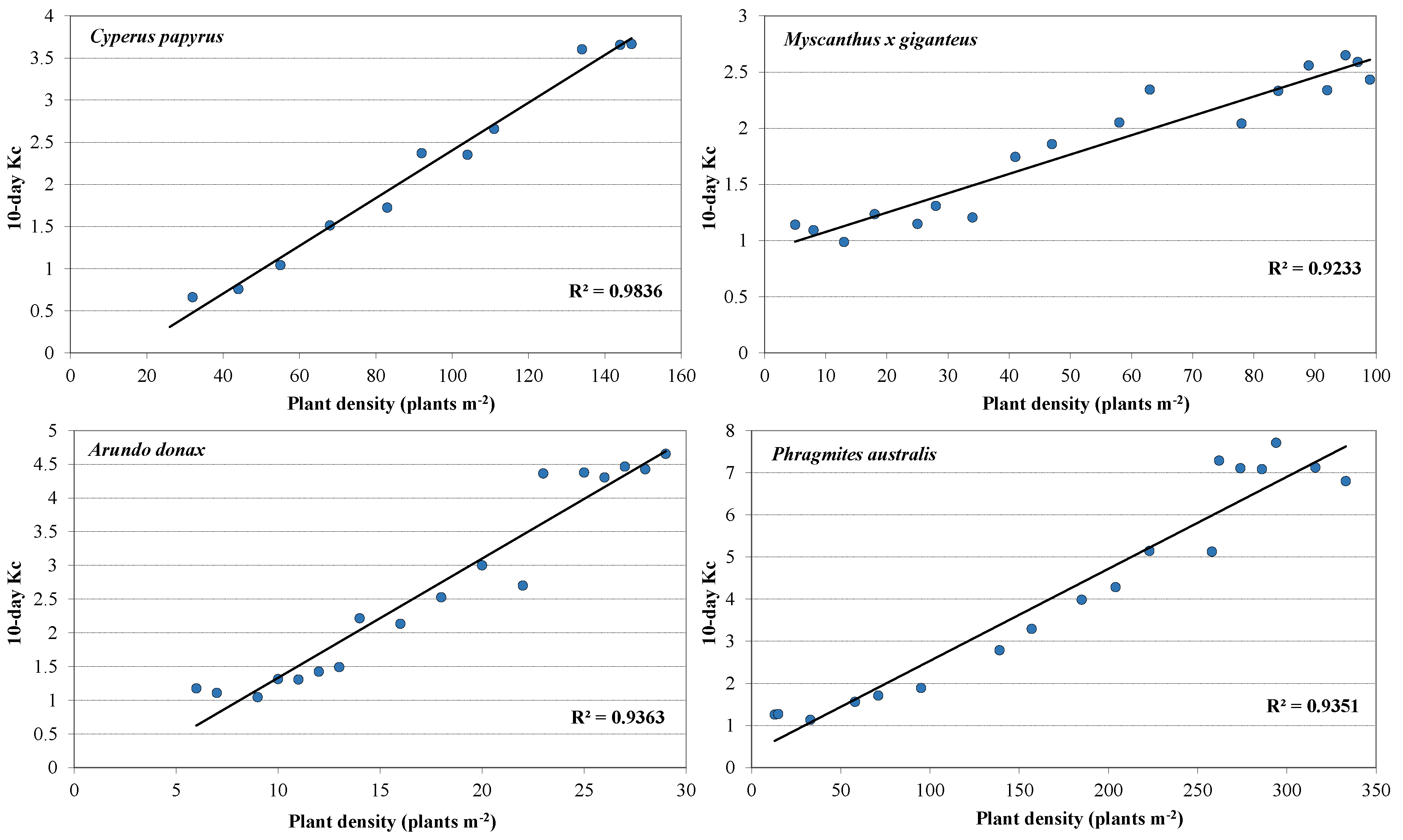
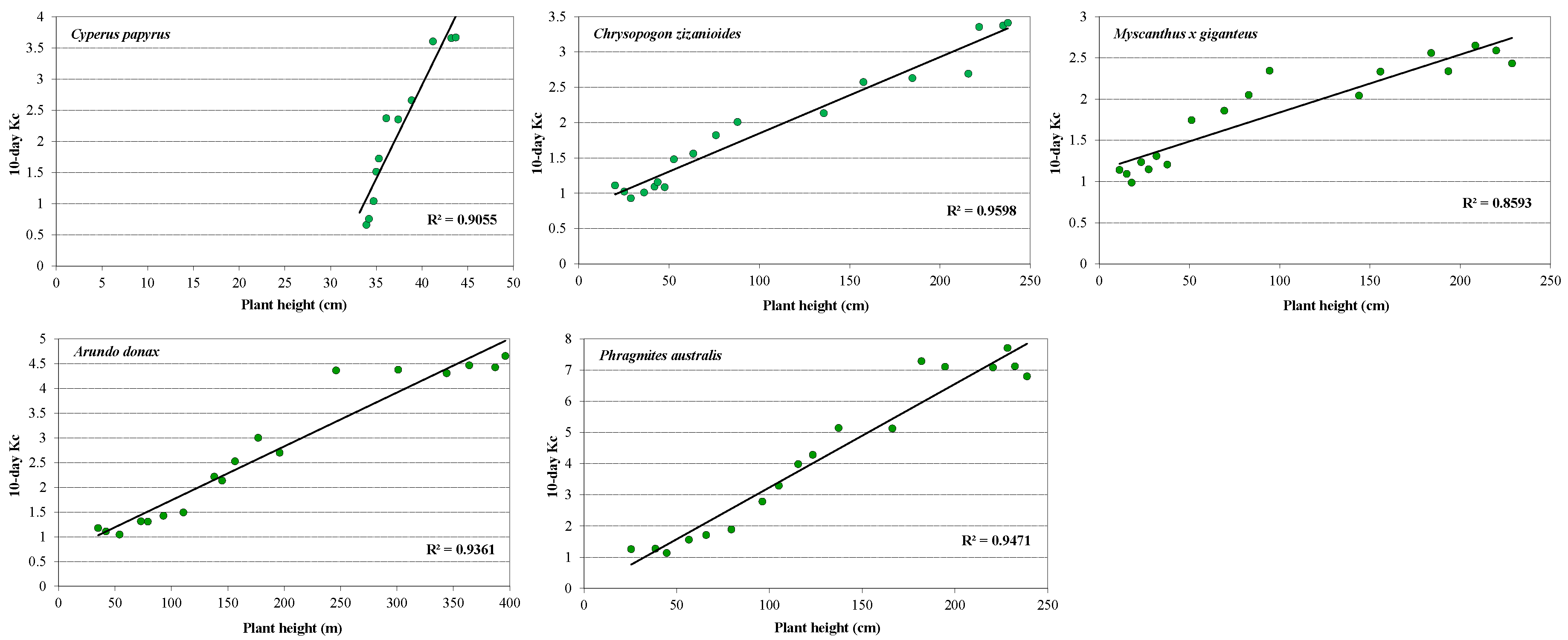
3.4. Crop Coefficients

The crop coefficient temporal patterns, for all species and in both growing seasons (Figure 9), are similar to the classical trapezium shape of Kc for agricultural crops [24], which shows the four growth stages (initial, crop development, mid-season, and late season).
In the initial growth stage, which for all species, except for C. papyrus, lasted about two months (April and May), the 10-day Kc varied between 0.93 (C. zizanioides in the last 10 days of April 2012) and 2.77 (P. australis in the second 10 days of May 2013).
The crop development stage varied in duration depending on the species and growing seasons: The minimum duration (five weeks, from the first 10-days of June 2013 to the first 10-days of July 2013) was found in M. giganteus, while the maximum duration (13 weeks, from the first 10-days of June 2012 to the first 10-days of September 2012) was observed in C. zizanioides. In the crop development stage, the 10-day Kc ranged from 0.66 (C. papyrus) to 7.29 (P. australis) in 2012 and from 1.74 (M. giganteus) to 6.69 (P. australis) in 2013.
In the overall mid-seasons, P. australis showed the highest average 10-day Kc value (7.10), followed by A. donax (4.45), C. papyrus (3.70), C. zizanioides (3.54), and M. giganteus (2.55).
During the plant senescence stage (late season), the 10-day Kc decreased until the end of November when average values, for both years, were about 3.57 for P. australis, 2.55 for A. donax, 1.78 for C. zizanioides, 1.46 for C. papyrus, and 1.09 for M. giganteus.
Regression analysis indicated a positive relationship between the 10-day Kc value found in 2012 and 2013 for P. australis, A. donax, C. zizanioides, and M. giganteus. As shown in Figure 10, the linear regression for P. australis and A. donax was higher than that for C. zizanioides and M. giganteus. This was due to the significant differences in dry biomass yield and bio-agronomic characters, between the two years, in C. zizanioides and M. giganteus. In fact, linear regression analysis showed that 10-Kc correlated strongly with phenological parameters (plant height and density), with a correlation factor ranging from 0.923 (M. giganteus) to 0.984 (C. papyrus) for plant density (Figure 11), and from 0.859 (M. giganteus) to 0.960 (C. zizanioides) for plant height (Figure 12).
The values recorded by A. donax, were lower than those reported by Tuttolomondo et al. [11], who reported a Kc of between 1.16 and 7.49 in a similar environment, probably due to minor “clothesline” and “oasis” effects in our study. These effects are particularly evident for small constructed wetlands [7,72] where an unlimited water supply coupled with energy advection to the surrounding area of macrophyte vegetation can lead to an increase in water loss by evapotranspiration.
The strong relationship between the size of the constructed wetlands and evapotranspiration was demonstrated by the results observed in P. australis. For this species, other studies [18,73] carried out in natural wetlands with extended surface areas of about 235 and 90,000 Ha, have shown ET rates ranging from 0.5 to 5.8 mm day−1 with mean Kc values of about 0.53 and 0.71, respectively, clearly lower than those estimated in our study (mean season Kc value of about 4.76).
It was not possible to show comparative Kc values for M. giganteus from other CWs, as no research was found on this specific subject. However, the Kc found for M. giganteus was in agreement with Triana et al. [70], who for M. giganteus cultivated in lysimeters in which the soil moisture was constantly maintained close to field capacity, reported Kc values ranging from 0.31 to 1.61.
Also, for C. zizanioides and C. papyrus a comparison of the Kc value was not possible since there are no available data in the literature for Mediterranean regions.

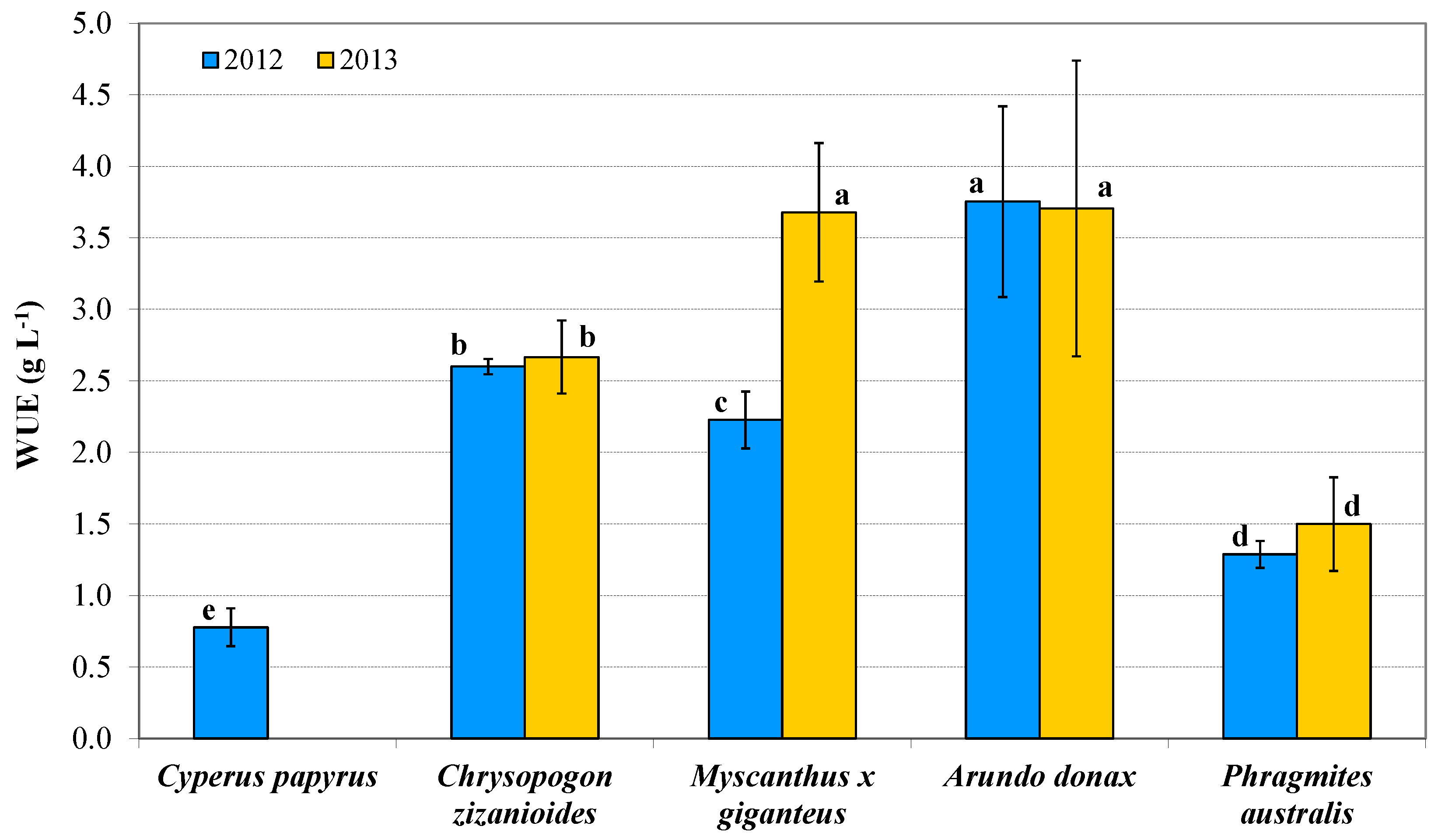
3.5. Water Use Efficiency Indices

For all species there were no significant differences between the WUE values determined in the two growing seasons (Figure 13) except for M. giganteus which increased the WUE value by about 65% between the 2012 and 2013 seasons. The highest value (3.68 g L−1) was comparable with results showed by A. donax (3.75 and 3.70 g L−1 in 2012 and 2013, respectively). The other species tested showed significantly lower average WUE values, about 29% (C. zizanioides), 62% (P. australis), and 79% (C. papyrus).
Generally, under optimum environmental conditions, the WUE of C4 plants is about twice as high as that of C3 plants [74]. However, there are several factors that affect the measurements of crop WUE, such as the variable quantity of harvestable parts of the biomass and the crop growing season [75]. These factors particularly affected the performances of A. donax and C. papyrus: (a) A. donax despite being a C3 plant showed comparable WUE values to M. giganteus (C4 plant). This is because in the autumn, the biomass losses in giant reed were very modest or absent, while in M. giganteus significant dry biomass losses were found; (b) the relative C. papyrus (C4 plant) reduced WUE was partially due to the delay in plant transplanting and the shorter growing season.
The WUE values determined for A. donax and M. giganteus were generally lower than those observed in other experimental studies carried out in a Mediterranean environment, in open fields with different irrigation treatments: Barbagallo et al. [76] and Cosentino et al. [77] found WUE values between 3.2 to 5.0 g L−1 for A. donax. Other authors [78,79] obtained WUE values ranging from 0.93 to 10 g L−1 for M. giganteus. This could be explained by the limited availability of water in open fields compared to CWs with permanently saturated conditions.
The WUE of P. australis showed values ranging from 1.29 to 1.50 g L−1, which were comparable to those obtained in other similar field experiments, ranging between 0.7 to 2.27 g L−1 [5,16,25,59].
Since there are few data available on the WUE of C. zizanioides in the literature, our results can only be compared with Barbagallo et al. [76] who in an open field irrigated with low quality water at 100% evapotranspiration restitutions, showed a mean value of about 1.3 g L−1.
Finally, information on the WUE of C. papyrus is still limited, and the studies that have dealt with this specific parameter [80,81] differ greatly in terms of climatic conditions or methodological approaches, thus preventing a meaningful comparison of the results.

4. Conclusions

Our study showed that P. australis was characterized by higher evapotranspiration rates (average value of about 17.31 mm day−1) followed by A. donax, C. zizanioides, C. papyrus, and M. giganteus, with average season values of about 11.23, 8.56, 7.86, and 7.35 mm day−1, respectively. As expected, the differences in ET observed between species can be explained by the photosynthetic cycles and the morphological parameters which showed a high correlation with Kc. The Kc time patterns, for all tested species, were similar to the classical trapezium shape of Kc for agricultural crops highlighting higher values than the latter, probably due to the unlimited water availability.
The ET process has not altered the salt concentrations in treated wastewater which have maintained, for the EC parameter, a slight degree of restriction for the irrigation use, as suggested by FAO guidelines [82].
An experimental investigation conducted in 2012 [11] in the same CWPP has proved the active role of tested species in the wastewater treatment detecting higher removal efficiencies of physico-chemical and microbiological parameters in vegetated beds than those obtained in unvegetated. The slight differences observed between the performances of vegetated beds highlighted the possibility to use successfully alternative species to the P. australis.
It should be noted that the small experimental plant may have led to over-estimating the plant evapotranspiration, due to the clothesline and oasis effects. However, comparing the results with other studies on evapotranspiration in small CWs, we believe that the data reported in this study are reliable. The results thus represent a useful guide for estimating the ET of P. australis, A. donax, C. zizanioides, C. papyrus, and M. giganteus and for calculating the Kc by the FAO-56 approach.
The high aboveground biomass values showed by A. donax, M. giganteus, C.zizanoides, and P. australis suggest that constructed wetlands used to treat wastewater have the potential to provide a sustainable bioenergy source without placing burdens on water resources or displacing other food or energy crops. Furthermore, the WUE indices calculated in this study could represent a reliable guide for selecting plants in CWs when the reusing treated wastewater is planned.

Author Contributions

The authors contributed with equal effort to the realization of the study. They were individually involved as follows: Writing—Review & Editing, M.M.; Data Curation and Investigation, M.M., A.M.; Conceptualization and Methodology, A.T., S.C. and G.L.C.; Visualization, D.V.; Supervision, S.B.

Funding

This research was funded by “Valorizzazione della risorsa idrica in ambiente Mediterraneo” financed by “Università di Catania—Piano per la ricerca di Ateneo 2016–2018—Linea di Intervento 2”. The experimental plant was built with funding by “MEDIWAT Project—Sustainable management of environmental issues related to water stress in Mediterranean islands” (cod:2G-MED09-262) financed by EU (MED Programme).

Conflicts of Interest

The authors declare no conflict of interest. The funders had no role in the design of the study; in the collection, analyses, or interpretation of data; in the writing of the manuscript, or in the decision to publish the results.

References

  1. Zhi, W.; Ji, G. Constructed Wetlands, 1991–2011: A Review of Research Development, Current Trends, and Future Directions. Sci. Total Environ. 2011, 441, 19–27. [Google Scholar] [CrossRef]
  2. Ventura, D.; Consoli, S.; Barbagallo, S.; Marzo, A.; Vanella, D.; Licciardello, F.; Cirelli, G.L. How to Overcome Barriers for Wastewater Agricultural Reuse in Sicily (Italy)? Water 2019, 11, 335. [Google Scholar] [CrossRef]
  3. Brisson, J.; Chazarenc, F. Maximizing pollutant removal in constructed wetlands: Should we pay more attention to macrophyte species selection? Sci. Total Environ. 2009, 407, 3923–3930. [Google Scholar] [CrossRef]
  4. Borin, M.; Milani, M.; Salvato, M.; Toscano, A. Evaluation of Phragmites australis (Cav.) Trin. evapotranspiration in Northern and Southern Italy. Ecol. Eng. 2011, 37, 721–728. [Google Scholar] [CrossRef]
  5. Milani, M.; Toscano, A. Evapotranspiration from pilot-scale constructed wetlands planted with Phragmites australis in a Mediterranean environment. J. Environ. Sci. Health Part A 2013, 48, 568–580. [Google Scholar] [CrossRef] [PubMed]
  6. El Hamouri, B.; Nazih, J.; Lahjouj, J. Subsurface-horizontal flow constructed wetland for sewage treatment under Moroccan climate conditions. Desalination 2007, 215, 153–158. [Google Scholar] [CrossRef]
  7. Kadlec, R.H.; Wallace, S.D. Treatment Wetlands, 2nd ed.; CRC Press: Boca Raton, FL, USA, 2009; 1016p. [Google Scholar]
  8. Fiener, P.; Auerswald, K.; Weigand, S. Managing erosion and water quality in agricultural water-sheds by small detention ponds. Agric. Ecosyst. Environ. 2005, 110, 132–142. [Google Scholar] [CrossRef]
  9. Xu, S.; Jaffè, P.R. Effects of plants on the removal of hexavalent chromium in wetland sediments. J. Environ. Qual. 2006, 35, 334–341. [Google Scholar] [CrossRef]
  10. Brix, H. Sludge Dewatering and Mineralization in Sludge Treatment Reed Beds. Water 2017, 9, 160. [Google Scholar] [CrossRef]
  11. Toscano, A.; Marzo, A.; Milani, M.; Cirelli, G.L.; Barbagallo, S. Comparison of removal efficiencies in Mediterranean pilot constructed wetlands vegetated with different plant species. Ecol. Eng. 2015, 75, 155–160. [Google Scholar] [CrossRef]
  12. Tuttolomondo, T.; Licata, M.; Leto, C.; Leone, R.; La Bella, S. Effect of plant species on water balance in a pilot-scale horizontal subsurface flow constructed wetland planted with Arundo donax L. and Cyperus alternifolius L.—Two-year tests in a Mediterranean environment in the West of Sicily (Italy). Ecol. Eng. 2015, 75, 79–92. [Google Scholar] [CrossRef]
  13. Toscano, A.; Hellio, C.; Marzo, A.; Milani, M.; Lebret, K.; Cirelli, G.L.; Langergraber, G. Removal efficiency of a constructed wetland combined with ultrasound and UV devices for wastewater reuse in agriculture. Environ. Technol. 2013, 34, 2327–2336. [Google Scholar] [CrossRef] [PubMed]
  14. Barbagallo, S.; Cirelli, G.L.; Consoli, S.; Licciardello, F.; Marzo, A.; Toscano, A. Analysis of treated wastewater reuse potential for irrigation in Sicily. Water Sci. Technol. 2012, 65, 2024–2033. [Google Scholar] [CrossRef] [PubMed] [Green Version]
  15. Consoli, S.; Milani, M.; Cirelli, G.L.; Barbagallo, S.; Marzo, A.; Vanella, D.; Toscano, A. Energy and water balance of a treatment wetland under mediterranean climatic conditions. Ecol. Eng. 2018, 116, 52–60. [Google Scholar] [CrossRef]
  16. Headley, T.R.; Davison, L.; Huett, D.O.; Müller, R. Evapotranspiration from subsurface horizontal flow wetlands planted with Phragmites australis in sub-tropical Australia. Water Res. 2012, 46, 345–354. [Google Scholar] [CrossRef]
  17. Anda, A.; Teixeira da Silva, J.A.; Soos, G. Evapotranspiration and crop coefficient of common reed at the surroundings of Lake Balaton, Hungary. Aquat. Bot. 2014, 116, 53–59. [Google Scholar] [CrossRef]
  18. Zhou, L.; Zhou, G. Measurement and modelling of evapotranspiration over a reed (Phragmites australis) marsh in Northeast China. J. Hydrol. 2009, 372, 41–47. [Google Scholar] [CrossRef]
  19. Borin, M.; Salvato, M. Effects of five macrophytes on nitrogen remediation and mass balance in wetland mesocosms. Ecol. Eng. 2012, 46, 34–42. [Google Scholar] [CrossRef]
  20. Calheiros, C.S.C.; Rangel, A.O.S.S.; Castro, P.M.L. Constructed wetland systems vegetated with different plants applied to the treatment of tannery wastewater. Water Res. 2007, 41, 1790–1798. [Google Scholar] [CrossRef]
  21. Pauliukonis, N.; Schneider, R. Temporal patterns in evapotranspiration from lysimeters with three common wetland plant species in the eastern United States. Aquat. Bot. 2001, 71, 35–46. [Google Scholar] [CrossRef]
  22. Papaevangelou, V.A.; Gikas, G.D.; Tsihrintzis, V.A. Evaluation of evapotranspiration in small on-site HSF constructed wetlands. J. Environ. Sci. Health A. 2012, 47, 766–785. [Google Scholar] [CrossRef] [PubMed]
  23. Barbagallo, S.; Cirelli, G.L.; Marzo, A.; Milani, M.; Toscano, A. Effect of different plant species in pilot constructed wetlands for wastewater reuse in agricultural. J. Agric. Eng. 2013, 44, 796–802. [Google Scholar]
  24. Allen, R.G.; Pereira, L.S.; Raes, D.; Smith, M. Crop Evapotranspiration: Guidelines for Computing Crop Requirements; FAO: Rome, Italy, 1998; 300p. [Google Scholar]
  25. Pedescoll, A.; Sidrach-Cardona, R.; Sánchez, J.C.; Bécares, E. Evapotranspiration affecting redox conditions in horizontal constructed wetlands under Mediterranean climate: Influence of plant species. Ecol. Eng. 2013, 58, 335–343. [Google Scholar] [CrossRef]
  26. Drexler, J.Z.; Anderson, F.E.; Snyder, R.L. Evapotranspiration rates and crop coefficients for a restored marsh in the Sacramento-San Joaquin Delta, California, USA. Hydrol. Process. 2008, 22, 725–735. [Google Scholar] [CrossRef]
  27. Barbera, A.C.; Cirelli, G.L.; Di Silvestro, I.; Pacifici, P.; Castiglione, V.; Toscano, A.; Milani, M. Growth and biomass production of different plant species in two different constructed wetland systems in Sicily. Desalination 2009, 246, 129–136. [Google Scholar] [CrossRef]
  28. Means, M.M.; Ahn, C.; Noe, G.B. Planting richness affects the recovery of vegetation and soil processes in constructed wetlands following disturbance. Sci. Total Environ. 2017, 579, 1366–1378. [Google Scholar] [CrossRef] [Green Version]
  29. Vymazal, J.; Kröpfelová, L. Growth of Phragmites australis and Phalaris arundinacea in constructed wetlands for wastewater treatment in the Czech Republic. Ecol. Eng. 2005, 25, 606–621. [Google Scholar] [CrossRef]
  30. Zygas, A.; Eheart, J.; Cai, X. Simulation and Optimization of a Constructed Wetland for Biomass Production and Nitrate Removal. J. Water Resour. Plan. Manag. 2014, 140, 1–10. [Google Scholar] [CrossRef]
  31. APHA, AWWA, AEF. Standard Methods for the Examination of Water and Wastewater; American Public Health Association (APHA), American WaterWorks Association (AWWA), and American Environment Federation (AEF): Washington, DC, USA, 2005. [Google Scholar]
  32. Rossa, B.; Tuffers, A.V.; Naidoo, G.; Von Willert, D.J. Arundo donax L. (Poaceae) a C3 species with unusually high photosynthetic capacity. Bot. Acta 1998, 111, 216–221. [Google Scholar] [CrossRef]
  33. Lewandowski, I.; Scurlock, J.M.O.; Lindvall, E.; Christou, M. The development and current status of perennial rhizomatous grasses as energy crops in the US and Europe. Biomass Bioenergy 2003, 25, 335–361. [Google Scholar] [CrossRef]
  34. Czako, M.; Marton, L. Subtropical and Tropical Reeds for Biomass (Chapter 16). In Energy Crops; The Royal Society of Chemistry: London, UK, 2010; pp. 322–340. [Google Scholar]
  35. Dudley, T.L. Arundo donax L. In Invasive Plants of California’s Wildlands; Bossard, C.C., Randall, J.M., Hoshovsky, M.C., Eds.; University of California Press: Berkeley, CA, USA, 2000; pp. 53–58. [Google Scholar]
  36. Idris, S.M.; Jones, P.L.; Salzman, S.A.; Croatto, G.; Allison, G. Evaluation of the giant reed (Arundo donax) in horizontal subsurface flow wetlands for the treatment of recirculating aquaculture system effluent. Environ. Sci. Pollut. Res. 2012, 19, 1159–1170. [Google Scholar] [CrossRef] [PubMed]
  37. Greef, J.M.; Deuter, M. Syntaxonomy of Miscanthus x giganteus GREEF et DEU. Angew. Bot. 1993, 67, 87–90. [Google Scholar]
  38. Hodkinson, T.R.; Renvoize, S.A.; Chase, M.W. Systematics in Miscanthus. Asp. Appl. Biol. 1997, 49, 189–198. [Google Scholar]
  39. Anderson, E.; Arundale, R.; Maughan, M.; Oladeinde, A.; Wycislo, A.; Voigt, T. Growth and agronomy of Miscanthus x giganteus for biomass production. Biofuels 2011, 2, 167–183. [Google Scholar] [CrossRef]
  40. Stander, W. Determination of the Highest Biomass Producing Plant Genera (C4 Grasses) of the World for Temperate Climates; Assessment Study for the Commission of the European Communities: Munich, Germany, 1989; 74p. [Google Scholar]
  41. Beale, C.V.; Bint, D.A.; Long, S.P. Leaf photosynthesis in the C4-grass Miscanthus x giganteus, growing in the cool temperate climate of southern England. J. Exp. Bot. 1996, 47, 267–273. [Google Scholar] [CrossRef]
  42. Vymazal, J. Plants used in constructed wetlands with horizontal subsurface flow: A review. Hydrobiologia 2011, 674, 133–156. [Google Scholar] [CrossRef]
  43. Garcia, J.; Aguirre, P.; Mueriego, R.; Hung, Y.; Ortiz, L.; Bayona, J.M. Initial contamination removal performance factor in horizontal flow reed beds used for treating urban wastewater. Water Res. 2004, 38, 1669–1678. [Google Scholar] [CrossRef]
  44. Worman, A.; Kronnas, V. Effect of pond shape and vegetation heterogeneity on flow and treatment performance of constructed wetlands. J. Hydrol. 2005, 301, 123–138. [Google Scholar] [CrossRef]
  45. Maltais-Landry, G.; Maranger, R.; Brisson, J.; Chazarenc, F. Nitrogen transformations and retention in planted and artificially aerated constructed wetlands. Water Res. 2009, 43, 535–545. [Google Scholar] [CrossRef]
  46. Xia, H.P. Ecological rehabilitation and phytoremediation with four grasses in oil shale mined land. Chemosphere 2004, 54, 345–353. [Google Scholar] [CrossRef]
  47. Jones, M.B. The photosynthetic characteristics of papyrus in a tropical swamp. Oecologia 1987, 71, 355–359. [Google Scholar] [CrossRef] [PubMed]
  48. Kuekenthal, G. Cyperaceae–Scirpoideae-Cyperae. In Das Pflanzenreich IV; 20 (Heft 101); Engler, A., Ed.; Wihelm Engleman: Leipzig, Germany, 1935; 671p. [Google Scholar]
  49. De Filipps, R.A. Cyperus. In Flora Europea; Tutin, T.G., Heywood, V.H., Burges, N.A., Moore, D.M., Valentine, D.H., Walters, S.M., Webb, D.A., Eds.; Cambridge University Press: Cambridge, UK, 1980; pp. 284–288. [Google Scholar]
  50. Gordon-Gray, K.D. Cyperaceae in Natal; National Botanical Institute: Pritoria, South Africa, 1995; 218p. [Google Scholar]
  51. Mabberley, D.J. The Plant Book. A Portable Dictionary of the Vascular Plants, 2nd ed.; Cambridge University Press: Cambridge, UK, 1997; 865p. [Google Scholar]
  52. Wunderlin, R.P. Guide to the Vascular Plants of Florida; University Press of Florida: Gainesville, FL, USA, 1998; 806p. [Google Scholar]
  53. Snyder, R.L.; Eching, S. Daily ETos, ETrs and HS ETo Calculator Using the ASCE-EWRI Method.xls; University of California, Davis: Davis, CA, USA, 2007; Available online: http://biomet.ucdavis.edu/Evapotranspiration/PMdayXLS/PMday.xls (accessed on 4 September 2019).
  54. Snyder, R.L.; Eching, S. Penman-Monteith Daily (24-h) Reference Evapotranspiration Equations for Estimating ETo, ETr and HS ETo with Daily Data; University of California, Davis: Davis, CA, USA, 2009; Available online: http://biomet.ucdavis.edu/Evapotranspiration/PMdayXLS/PMdayDoc.pdf (accessed on 4 September 2019).
  55. ASCE-EWRI. The ASCE Standardized Reference Evapotranspiration Equation. In Environmental and Water Resources Institute (EWRI) of the American Society of Civil Engineers (ASCE) Standardization of Reference Evapotranspiration Task Committee Final Report; Allen, R.G., Walter, I.A., Elliott, R., Howell, T.A., Itenfisu, D., Jensen, M.E., Eds.; ASCE-EWRI: Reston, VA, USA, 2005; 213p. [Google Scholar]
  56. Sinclair, T.R.; Tanner, C.B.; Bennett, J.M. Water use efficiency in crop production. Bioscience 1984, 34, 40–60. [Google Scholar] [CrossRef]
  57. Borin, M.; Barbera, A.C.; Milani, M.; Molari, G.; Zimbone, S.M.; Toscano, A. Biomass production and N balance of giant reed (Arundo donax L.) under high water and N input in Mediterranean environments. Eur. J. Agron. 2013, 51, 117–119. [Google Scholar] [CrossRef]
  58. Kuusemets, V.; Lõhmus, K. Nitrogen and Phosphorus Accumulation and Biomass Production by Scirpus sylvaticus and Phragmites australis in a Horizontal Subsurface Flow Constructed Wetland. J. Environ. Sci. Health Part A 2005, 40, 1167–1175. [Google Scholar] [CrossRef]
  59. Mueller, L.; Behrendt, A.; Schalitz, G.; Schindler, U. Above ground biomass and water use efficiency of crops at shallow water tables in a temperate climate. Agric. Water Manag. 2005, 25, 117–136. [Google Scholar] [CrossRef]
  60. Eid, E.M.; Shaltout, K.H. Monthly variations of trace elements accumulation and distribution in above- and below-ground biomass of Phragmites australis (Cav.) Trin. Ex Steudel in Lake Burullus (Egypt): A biomonitoring application. Ecol. Eng. 2014, 73, 17–25. [Google Scholar] [CrossRef]
  61. Zub, H.W.; Brancourt-Hulmel, M. Agronomic and physiological performances of different species of Miscanthus, a major energy crop. A Review. Agron. Sustain. Dev. 2010, 30, 201–214. [Google Scholar] [CrossRef]
  62. Zhao, F.; Yang, W.; Zeng, Z.; Li, H.; Yang, X.; He, Z.; Gu, B.; Rafiq, M.T.; Peng, H. Nutrient removal efficiency and biomass production of different bioenergy plants in hypereutrophic water. Biomass Bioenergy 2012, 42, 212–218. [Google Scholar] [CrossRef]
  63. Truong, P.; Smeal, C. Research, Development and Implementation of Vetiver System for Wastewater Treatment: GELITA Australia; Technical Bulletin No. 2003/3; Pacific Rim Vetiver Network. Office of the Royal Development Projects Board: Bangkok, Thailand, 2003. [Google Scholar]
  64. Perbangkhem, T.; Polprasert, C. Biomass production of papyrus (Cyperus papyrus) in constructed wetland treating low-strength domestic wastewater. Bioresour. Technol. 2010, 101, 833–835. [Google Scholar] [CrossRef]
  65. Mnaya, B.; Asaeda, T.; Kiwango, Y.; Ayubu, E. Primary production in papyrus (Cyperus papyrus L.) of Rubondo Island, Lake Victoria, Tanzania. Wetl. Ecol. Manag. 2007, 15, 269–275. [Google Scholar] [CrossRef]
  66. Rozkošný, M.; Šálek, J.; Šálek, J. Water balance of the constructed wetlands – a study of the macrophyte´s evapotranspiration. In Proceedings of the 10th International Conference Wetland Systems for Water Pollution Control, Lisbon, Portugal, 23–29 September 2006. [Google Scholar]
  67. Herbst, M.; Kappen, L. The ratio of transpiration versus evaporation in a reed belt as influenced by weather conditions. Aquat. Bot. 1999, 63, 113–125. [Google Scholar] [CrossRef]
  68. Fermor, P.M.; Hedges, P.D.; Gilbert, J.C.; Gowing, D.J.G. Reedbed evapotranspiration rates in England. Hydrol. Process. 2001, 15, 621–631. [Google Scholar] [CrossRef]
  69. Chazarenc, F.; Merlin, G.; Gonthier, Y. Hydrodynamics of horizontal subsurface flow constructed wetlands. Ecol. Eng. 2003, 21, 165–173. [Google Scholar] [CrossRef]
  70. Triana, F.; Nassi o Di Nasso, N.; Ragaglini, G.; Roncucci, N.; Bonari, E. Evapotranspiration, crop coefficient and water use efficiency of giant reed (Arundo donax L.) and miscanthus (Miscanthus x giganteus Geef et Deu.) in a Mediterranean environment. GBC Bioenergy 2014, 7, 811–819. [Google Scholar]
  71. Kyambadde, J.; Kansiime, F.; Dalhammar, G. Nitrogen and phosphorus removal in substrate-free pilot constructed wetlands with horizontal surface flow in Uganda. Water Air Soil Pollut. 2005, 165, 37–59. [Google Scholar] [CrossRef]
  72. Allen, R.G.; Pereira, L.S.; Howell, T.A.; Jensen, M.E. Evapotranspiration information reporting: I. Factors governing measurement accuracy. Agric. Water Manag. 2011, 98, 899–920. [Google Scholar] [CrossRef] [Green Version]
  73. Peacock, C.E.; Hess, T.M. Estimating evapotranspiration from a reed bed using the Bowen ratio energy balance method. Hydrol. Process. 2004, 18, 247–260. [Google Scholar] [CrossRef]
  74. Stanhill, G. Water use efficiency. Adv. Agron. 1986, 39, 53–85. [Google Scholar]
  75. Berndes, G. Bioenergy and water—The implications of large-scale bioenergy production for water use and supply. Glob. Environ. Chang. 2002, 12, 253–271. [Google Scholar] [CrossRef]
  76. Barbagallo, S.; Barbera, A.C.; Cirelli, G.L.; Milani, M.; Toscano, A. Reuse of constructed wetland effluents for irrigation of energy crops. Water Sci. Technol. 2014, 70, 1465–1472. [Google Scholar] [CrossRef]
  77. Cosentino, S.L.; Patanè, C.; Sanzone, E.; Copani, V.; Foti, S. Effects of soil water content and nitrogen supply on the productivity of Miscanthus x giganteus Greef et Deu. in a Mediterranean environment. Ind. Crops Prod. 2007, 25, 75–88. [Google Scholar] [CrossRef]
  78. Mantineo, M.; D’Agosta, G.M.; Copani, V.; Patanè, C.; Cosentino, S.L. Biomass yield and energy balance of three perennial crops for energy use in the semi-arid Mediterranean environment. Field Crops Res. 2009, 114, 204–213. [Google Scholar] [CrossRef]
  79. Christou, M.; Mardikis, M.; Alexopoulou, E.; Cosentino, S.L.; Copani, V.; Sanzone, E. Environmental studies on Arundo donax. In Proceedings of the 8th International Conference on Environmental Science and Technology, Lemnos Island, Greece, 8–10 September 2003; Curran Associates Inc.: Red Hook, NY, USA, 2003; pp. 102–110. [Google Scholar]
  80. Morrison, E.H.J.; Harper, D.M. Ecohydrological principles to underpin the restoration of Cyperus papyrus at Lake Naivasha, Kenya. Ecohydrol. Hydrobiol. 2009, 9, 83–97. [Google Scholar] [CrossRef]
  81. Aiello, R.; Cirelli, G.L.; Consoli, S.; Licciardello, F.; Toscano, A. Risk assessment of treated municipal wastewater reuse in Sicily. Water Sci. Technol. 2013, 67, 89–98. [Google Scholar] [CrossRef] [Green Version]
  82. Ayers, R.S.; Westcot, D.W. Water Quality for Agriculture; FAO Irrigation and Drainage, Paper 29; Food and Agriculture Organization: Rome, Italy, 1985. [Google Scholar]
Figure 1. Layout of pilot plant constructed wetland. Cyperus papyrus was planted in horizontal sub surface flow (H-SSF)1 and H-SSF7, Chrysopogon zizanioides in H-SSF2 and H-SSF8, Miscanthus x giganteus in H-SSF3 and H-SSF9, Arundo donax in H-SSF4 and H-SSF10, and Phragmites australis in H-SSF5 and H-SSF11, while H-SSF6 and H-SSF12 are unplanted.
Water 11 02159 g001
Figure 2. Pictures of Cyperu papyrus (a), Chrysopogon zizanioides (b), Miscanthus x giganteus (c), Arundo donax (d), and Phragmites australis (e).
Water 11 02159 g002
Figure 3. Trends of plant height and density (of C. papyrus, C. zizanioides, M. giganteus, A. donax, and P. australis) and number of leaves (total and dead) and stem diameter (of M. giganteus, A. donax, and P. australis) during 2012 growing season.
Water 11 02159 g003
Figure 4. Total aerial dry matter of the herbaceous species in December 2012 and 2013 (different letters indicate significant differences at p < 0.05).
Water 11 02159 g004
Figure 5. ET0 daily rates during 2012 and 2013 observation periods.
Water 11 02159 g005
Figure 6. Trend of meteorological data and 10-day average ET0, ETcon, and ET for C. papyrus, C. zizanioides, M. giganteus, A. donax, and P. australis during 2012 (a) and 2013 (b) observation periods.
Water 11 02159 g006
Figure 7. Cumulative ET0, ETcon, and ET for C. papyrus, C. zizanioides, M. giganteus, A. donax, and P. australis during 2012 (a) and 2013 (b) observation periods.
Water 11 02159 g007
Figure 8. Relationship between ET0 and ET for C. papyrus, C. zizanioides, M. giganteus, A. donax, and P. australis in 2012 and 2013 observation periods.
Water 11 02159 g008
Figure 9. 10-day Kc of C. papyrus, C. zizanioides, M. giganteus, A. donax, and P. australis during 2012 (a) and 2013 (b) observation periods.
Water 11 02159 g009
Figure 10. Relationship between 10-day crop coefficient (Kc) for C. zizanioides (a), M. giganteus (b), A. donax (c), and P. australis (d) in 2012 and 2013 observation periods.
Water 11 02159 g010
Figure 11. Relationship between 10-day Kc and plant density for C. papyrus, M. giganteus, A. donax, and P. australis from April to September 2012.
Water 11 02159 g011
Figure 12. Relationship between 10-day Kc and plant height for C. papyrus, V.zizanioides, M. giganteus, A. donax, and P. australis from April to September 2012.
Water 11 02159 g012
Figure 13. Water use efficiency (WUE) of the herbaceous species in December 2012 and 2013 (different letters indicate significant differences at p < 0.05).
Water 11 02159 g013
Table 1. Mean influent (±SD) pollutant concentrations of all the constructed wetland (CW) beds during 2012 and 2013 season.
ParametersUnitYear
20122013
Mean±SDMean±SD
TSSmg L−178.0(±61.4)35.5(±16.7)
BOD5mg L−1not detected30.8(±3.9)
CODmg L−167.9(±40.4)50.6(±2.6)
NH4-Nmg L−17.1(±4.5)11.4(±4.8)
NO2-Nmg L−10.3(±0.2)0.3(±0.1)
NO3-Nmg L−16.7(±4.7)1.0(±0.4)
Norgmg L−11.4(±0.7)2.4(±0.9)
TNmg L−115.6(±7.5)15.1(±4.6)
PO4-Pmg L−13.3(±1.3)7.5(±0.9)
Table 2. Monthly meteorological data for the calculation of evapotranspiration (ET0) in the two years.
YearMonthCumulative RainAbsolute Minimum Air TemperatureAbsolute Maximum Air TemperatureAverage Air TemperatureAverage Wind SpeedAverage Relative HumidityAverage Solar Radiation
mm°C°C°Cms−1%MJm−2d−1
2012April66.01.527.113.31.873.922.2
May5.63.929.516.81.061.926.7
June0.08.237.523.10.948.129.9
July4.413.443.426.30.847.527.6
August0.013.942.226.10.849.224.2
September8.011.735.622.00.766.019.6
October18.23.334.519.00.675.313.5
November0.63.425.614.40.783.58.4
Average Season102.8 *12.528.120.10.963.15253.2 *
2013April3.03.525.313.70.673.921.3
May1.04.430.517.01.064.124.8
June0.07.837.320.90.952.629.7
July0.010.239.923.90.954.927.3
August0.014.437.424.81.457.724.1
September62.48.834.321.11.171.118.8
October9.26.433.619.20.971.914.5
November61.4−1.626.712.40.979.29.6
Average Season137.0 *11.827.019.21.065.65196.1 *
* Cumulated value.
Table 3. Mean values and standard deviation (±SD) of plant height, basal stem diameter, total leaves, and plant density of herbaceous species at the beginning (initial) and end (final) of each investigation year.
Plant SpeciesYearPhasePlant HeightBasal Stem DiameterTotal LeavesPlant Density
(cm)(mm)(No Plant−1)(Plants m−2)
Mean ± SDMean ± SDMean ± SDMean ± SD
Cyperus papyrus2012Initial33.2 ± 2.4(a)--26.0 ± 2.8(b)
Final46.3 ± 4.5(a)--156.0 ± 6.6(a)
2013Initial----
Final----
Chrysopogon zizanoides2012Initial20.1 ± 1.8(c)--5.5 ± 0.0
Final251.2 ± 14.8(a)--5.5 ± 0.0
2013Initial58.1 ± 3.7(b)--5.5 ± 0.0
Final263.5 ± 3.5(a)--5.5 ± 0.0
Myscanthus x giganteus2012Initial11.2 ± 0.9(d)3.3 ± 0.3(b)4.8 ± 1.1(b)5.0 ± 1.7(d)
Final247.3 ± 11.0(b)7.1 ± 0.5(a)14.8 ± 2.1(a)105.0 ± 11.0(b)
2013Initial65.6 ± 3.6(c)4.8 ± 0.4(b)7.5 ± 2.2(b)64.6 ± 3.5(c)
Final286.9 ± 21.3(a)8.2 ± 0.5(a)16.2 ± 1.6(a)144.5 ± 6.7(a)
Arundo donax2012Initial35.1 ± 2.1(c)6.1 ± 0.4(c)6.2 ± 1.3(c)6.0 ± 1.4(c)
Final437.3 ± 24.5(a)23.3 ± 2.5(a)42.8 ± 8.9(a)30.5 ± 4.9(a)
2013Initial91.9 ± 6.3(b)13.3 ± 1.5(b)12.1 ± 3.9(b)14.4 ± 2.7(b)
Final441.5 ± 37.3(a)23.9 ± 3.2(a)42.9 ± 7.4(a)32.0 ± 3.1(a)
Phragmites australis2012Initial25.4 ± 3.1(c)2.7 ± 0.4(b)4.3 ± 0.8(b)13.3 ± 3.1(c)
Final248.7 ± 8.1(a)8.1 ± 1.1(a)17.7 ± 2.1(a)364.2 ± 18.6(a)
2013Initial77.3 ± 5.3(b)4.6 ± 0.9(b)5.9 ± 1.1(b)108.1 ± 6.9(b)
Final252.6 ± 13.4(a)8.7 ± 1.0(a)18.3 ± 2.0(a)382.0 ± 16.5(a)
In each parameter and in each species, values followed by different letters are significantly different (p < 0.05).

