Three-Dimensional Numerical Method for Simulating Large-Scale Free Water Surface by Massive Parallel Computing on a GPU

1
School of River and Ocean Engineering, Chongqing Jiaotong University, Chongqing 400016, China
2
State Key Laboratory of Water Resources and Hydropower Engineering Science, Wuhan University, Wuhan 430072, China
*
Author to whom correspondence should be addressed.
Water 2019, 11(10), 2121; https://doi.org/10.3390/w11102121
Submission received: 5 September 2019
/
Revised: 30 September 2019
/
Accepted: 9 October 2019
/
Published: 13 October 2019
(This article belongs to the Section Hydraulics and Hydrodynamics)
Abstract
:Water wave dynamics and its engineering application have always been a key issue in the field of hydraulics, and effective and efficient numerical methods need to be proposed to perform three-dimensional (3-D) simulation of large-scale water fluctuation in engineering practice. A single-phase free-surface lattice Boltzmann method (SPFS-LB method) is coupled with a large-eddy simulation approach for simulating large-scale free water surface flows, and the simulation is accelerated on a GPU (graphic processing unit). The coupling model is used to simulate the evolution process of dam-break wave after complete and partial dam-break. The formation mechanism of horizontal and vertical vortices in water after partial dam-break and the advance and evolution process of dam-break flow on non-contour riverbed are analyzed. The method has been verified to be reasonable and can obtain a more accurate time curve of water level fluctuation. Applying this method to practical arch dams, discharge coefficients consistent with empirical formulas can be obtained by comparison and analysis, and the surface flow phenomena (such as tongue diffusion, surface fragmentation, and surface fusion) can be well simulated by this method. In addition, based on the key technology of parallel computing on a GPU, the implementation of the SPFS-LB model on a GPU unit achieves tens of millions of lattice updates per second, which is over fifty times higher than that on a single CPU chip. It is proved that the proposed method for large-scale water fluctuations can be used to study practical engineering problems. The mathematical model method realizes the efficient and accurate simulation of practical physical problems.
1. Introduction
Water fluctuation phenomena such as waves and tiding exist widely in nature. Water wave dynamics on large scales is one of the research focuses of hydraulic projects, such as the surges generated by landslides [1], water-level fluctuations in surge chambers [2], and flood discharge of spillways [3]. The above phenomena are large-scale free-surface (LS-FS) flows with the following features: (1) the viscosity and density ratios of the two phases are large; (2) the movements of the interface between the two phases are dominated by the phase with larger density and viscosity; (3) the capillary effects on flows can be neglected. These hydraulic problems are quite complex, and they are vital to the safe operation and stability of the hydraulic projects. Therefore, an intensive study on effective and efficient simulation of LS-FS flows is necessary.
At present, the general methods for studying LS-FS flows are mainly two-dimensional (2-D) numerical models, especially shallow water equations for simulating planar flows. 2-D numerical simulations have been one of the most important tools to analyze LS-FS flows, such as flows in rivers, reservoirs, or ocean [4,5]. However, the above 2-D numerical models cannot analyze vertical velocity variation, and they cannot be used to simulate the breaking down, merging, and expanding of water surface, which greatly limits the applications of 2-D models in the field of hydraulic projects. Therefore, the free surface flows with obvious three-dimensional (3-D) features should be simulated by 3-D methods. Traditionally, 3-D numerical methods developed for free-surface flows are mainly based on gas–liquid two-phase flow models [6], interface tracking models (common approaches include Volume of fluid (VOF) [7], level set [8], phase field [9]), and interface capturing models (including moving mesh approach [10], marker and cell (MAC) method [11], and particle-in-cell approach [12]). However, simulating LS-FS flows, particularly those in the area of hydraulic projects, requires a remarkable amount of computing resources, while it is challenging to maintain the stability and accuracy of the simulation.
The single phase free surface lattice Boltzmann (SPFS-LB) model was originally proposed by Thürey in 2003 [13]. The SPFS-LB model is more suitable to simulate 3-D LS-FS flows in comparison with traditional 3-D numerical models in which both gas and fluid are simulated to properly reflect the interface boundary conditions [13,14]. The SPFS-LB model only simulates the water flows, without consideration of air influence, so the consumption of computation resources is low. In addition, this model is on the basis of lattice Boltzmann (LB) method, which has the advantages of a simple algorithm, good parallelism, easily programing, and simple implementation of boundary conditions [15].
The design of graphic processing units (GPUs) consists of a high-speed super-long pipeline and massively parallel processing in hardware, and its frame is naturally consistent with features of the LB algorithm. At present, the accelerated computing research of GPU-based LB methods has made certain progress. In reference [16], the implementation of the LB method for shallow water flows on a GPU unit can realize billions of lattice updates per second, which is hundreds of times higher than that on a single CPU core. However, there are rare research reports on simulating large-scale 3-D wave movements by the SPFS-LB model in hydraulic projects using GPUs; therefore, this paper investigates this field.
In this paper, the SPFS-LB model is coupled with the large-eddy simulation (LES) method for analyzing the LS-FS flows, and the method is implemented on a GPU. Firstly, the coupling model is used to simulate sudden whole dam-break flow, partial dam-break flow, and dam-break flow over a triangular step. To validate the accuracy of the proposed model in simulating large-scale free surface flows, the simulated water surface profiles, velocity distribution, and the process of waves are compared with the reference data. The SPFS-LB model is applied to analyze the flood discharge of an arch dam for demonstrating its capability for simulating practical flow problems. In the Appendix A, the algorithm is implemented on a GPU to realize efficient computation. Eventually, our work shows that this new method can simulate LS-FS flows in actual project problems accurately and efficiently.
2. Method
2.1. Lattice Boltzmann Method
In the Lattice Boltzmann method, the particle movement of the simulated fluid is dispersed on several fixed directions, and the discrete particle velocity on the direction i is expressed by ei. Through solution and statistics of particle distribution function fi corresponding to various discrete velocities, the macroscopic variables of the fluid such as density and momentum of the fluid are obtained.
Take the commonly used D3Q19 model as an example, the LB equation with MRT collision term can be described as:
where refers to the discrete distribution functions related to location r and time ; refers to the forcing term; refers to the moment of distribution functions (see reference [17] for details). The relationship among m, transfer matrix M, and distribution function f can be expressed as:
Diagonal collision matrix can be expressed as:
where , , , , . refers to kinematic viscosity.
2.2. Single-Phase Free Surface Lattice Boltzmann Model
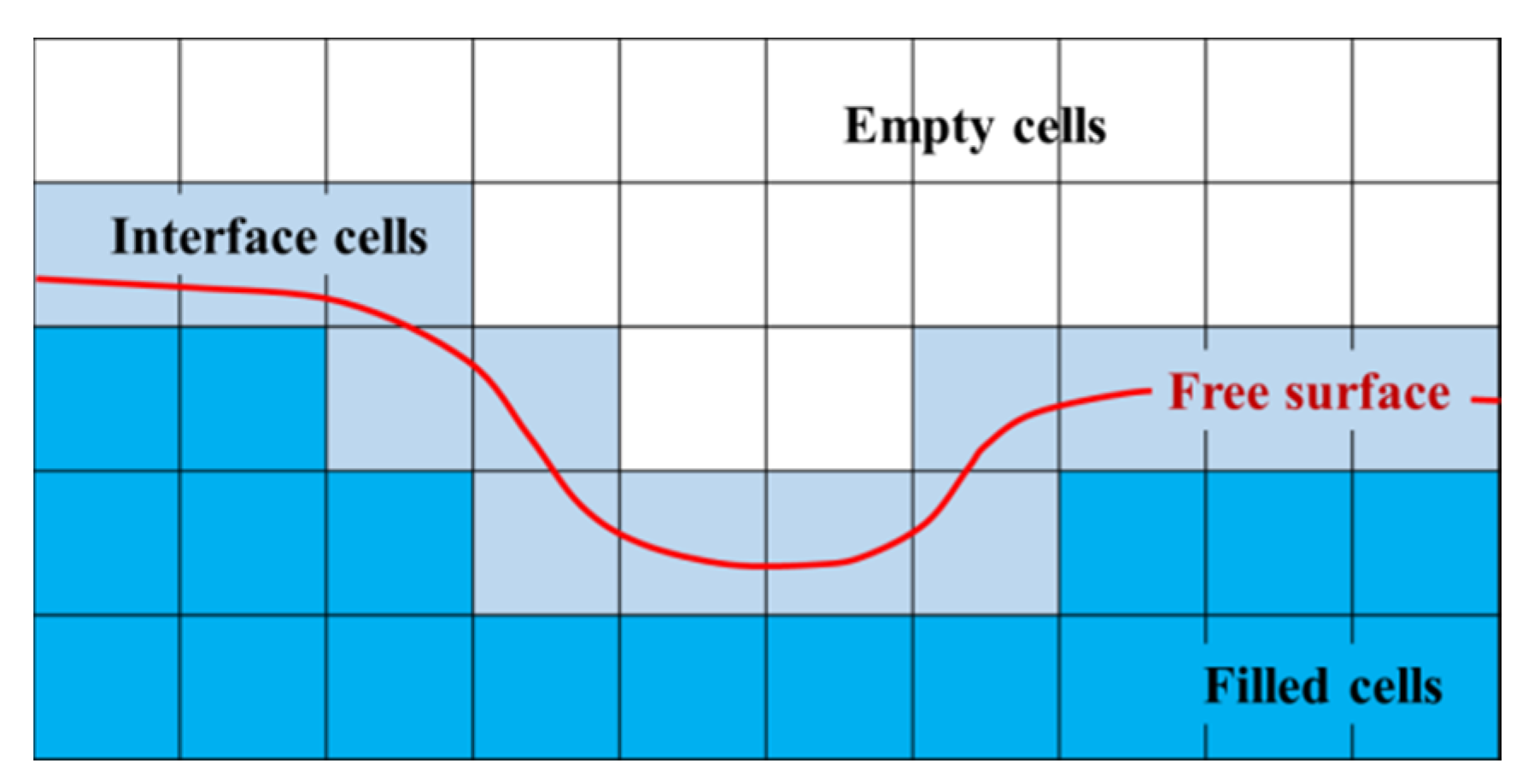
The SPFS-LB model is based on the following assumptions: (1) the effects of the gas on the fluid can be neglected; (2) the gas can achieve equilibrium state immediately after the change of the fluid state; (3) the fluid and gas are separated by a closed layer of the interface cells. The SPFS-LB model divides the computational cells into filled cell, interface cell, and empty cell. Moreover, the filled cell is fully filled with simulated fluid, and the definition of variables and the evolution process of distribution functions are the same as those in the conventional single-phase LB method. The interface cell is only partially filled with liquid, while the empty cell includes no liquid, and no physical quantity needs to be defined, as shown in Figure 1. All the three cells have a defined volume fraction , where m and refer to the mass and density of the cell, and the value range of the filled cell, interface cell, and empty cell are 1, 0–1, and 0, respectively.
2.2.1. Mass Flow Computation
In the SPFS-LB model, the inflow mass and outflow mass of a cell are computed to update its volume fraction ; then, the interval of is judged to change its cell type. In the LB method, the mass flow can be simply obtained from the two antiparallel particle distribution functions fi and finv(i), where einv(i) = −ei, and denotes the mass variable quantity on direction along the particle velocity [11].
Accordingly, the mass of the interface cell at x can be updated via Equation (5). It can be validated that the mass update computation by Equation (5) complies with the law of conservation of mass [13].
2.2.2. Reconstruction of Interface Cells
The filled cell is surrounded with other filled or interface cells. Profiting from a full set of distribution functions, the LB propagation and LB collision can normally be performed here. However, the interface cell is always surrounded with empty cells, so the distribution functions of the interface cell need to be reconstructed according to the macroscopic boundary conditions after LB propagation. Based on assumption 2, the unknown distribution functions of the interface cell can be reconstructed through Equation (6) [13].
where and u refer to pressure and velocity at position x, respectively. In addition, to balance the forces given by the gas pressure and velocity at interface, the distribution functions whose discrete velocity direction ei satisfies ei·n < 0 shall be reconstructed [13], where n refers to the surface normal direction and can be obtained by the second-order central difference approximation .
2.2.3. Mass Allocation
After updating the mass m and volume fraction of the interface cell, the interface cell requires special treatment. If , the interface cell is converted to a filled cell, and the excess mass needs to be allocated to the surrounding empty cells and interface cells. Accordingly, the adjacent empty cells are converted to interface cells after getting mass from the new filled cell. The macroscopic density and velocity of the new emerging interface cells can be gained by averaging the macroscopic variables of the surrounding interface cells and filled cells, and the distribution functions can be initialized based on equilibrium distribution functions [14]. Likewise, if the of an updated interface cell drops below zero, it is converted to an empty cell. The negative mass of this cell shall be complemented to 0 by the adjacent filled cells and interface cells, and the adjacent filled cells shall be transformed into interface cells. When the excess mass is distributed from excessive or insufficient cells to surrounding interface cells, the proportion should be calculated according to the dot product between the distribution direction and the interface normal direction. For example, the excess mass of an interface cell at position x distributed to the cell at x + ei is [13]:
where , , .As the mass allocation is completed and the cell type is converted, the interface moves accordingly.
2.3. Large Eddy Simulation Based on the LB Method
Turbulence exists widely in the field of hydraulic projects. For improving practicability, a turbulence simulation method shall be introduced to this SPFS-LB model. In the text, the subgrid-scale model based on LES is applied. This method separates the physical variables of flows into two parts by a certain filter function: small-scale variables and large-scale variables [18]. For instance, a variable can be divided into and , where is the filtered large-scale part of using the filter function G, and is the small-scale pulsation being modeled.
By filtering Equation (1) using G and assuming , Equation (8) should be obtained:
As for LES based on the subgrid-scale model, the viscosity can be understood as , where and refer to molecular viscosity and turbulence viscosity (or eddy viscosity) respectively. The turbulence viscosity can be expressed as , where , and refer to the model parameters of filter width and strain rate tensor, respectively, and S can be obtained directly from the nonequilibrium moments . See reference [18] for more details.
3. Testing and Discussion
In this section, the SPFS-LB model is used to simulate whole and partial dam-break waves. Through comparative analysis between the simulated results and the reference data, it turns out that the present model can simulate the large-scale free surface effectively. The 3D SPFS-LB model can reflect more abundant hydrodynamic information compared with the traditional 1D or 2D methods. If not otherwise stated, the acceleration of gravity, water density, and viscosity are set as , , and , respectively.
3.1. Sudden Whole Dam-Break Flow
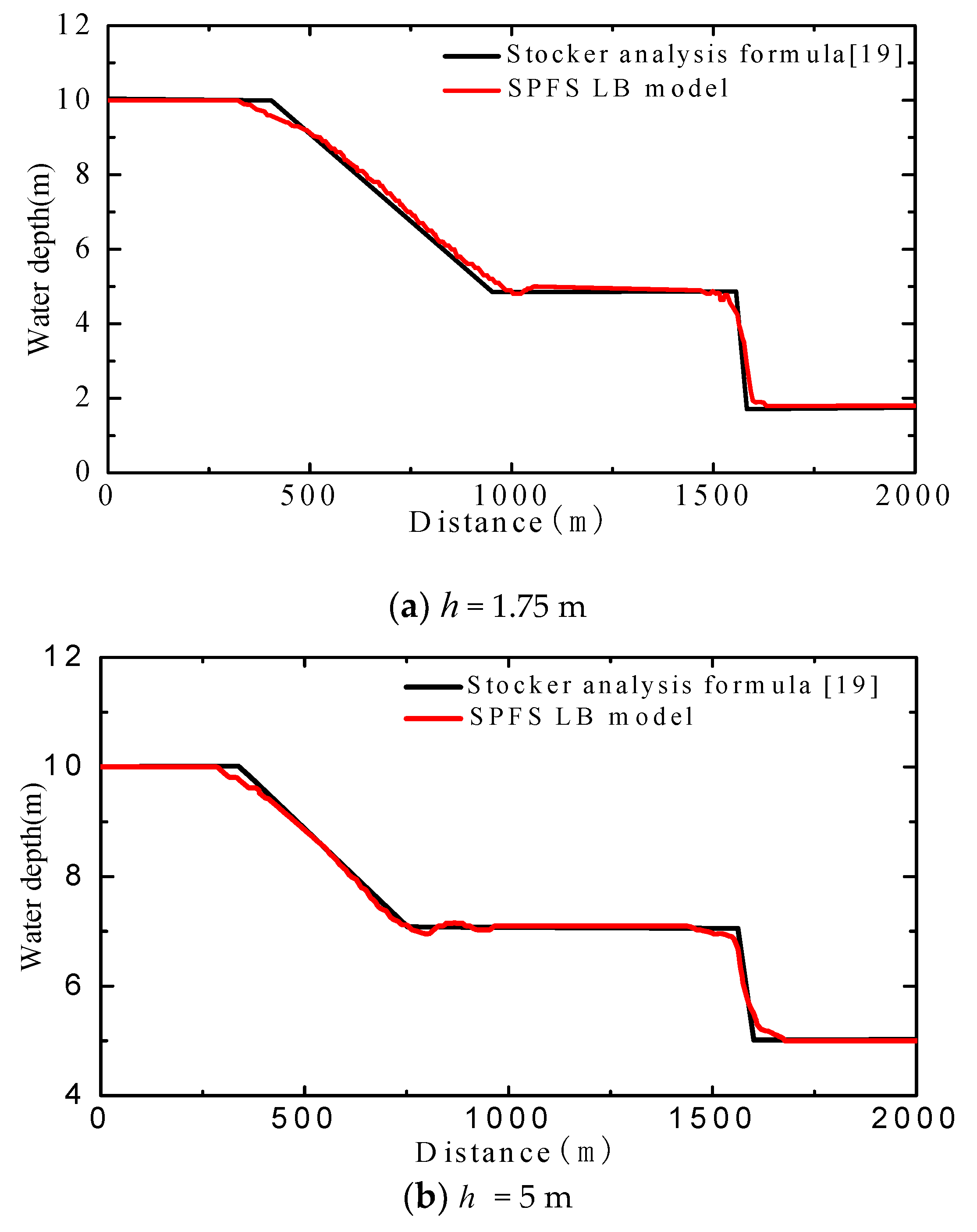
The sudden whole dam-break flow is a classic test case with an analytical solution, and it is simulated to make a comparison between the numerical results and the analytical results. It is assumed that a horizontal river channel is 2000 m long with equivalent width and a perfectly smooth bottom. The dam is located in the middle of the channel, and the water depth of upstream reservoir is H = 10 m. The water surface profile of the dam-break wave is simulated with the downstream water depth of h = 5 m and 1.75 m, and compared with the analytical values [19]. The simulations are conducted on a uniform lattice 10,000 × 50 (Δx = 0.2 m). The left side, right side, and bottom of the computational domain are treated as nonslip wall boundary conditions.
Figure 2 indicates that the simulated water surface profile based on the SPFS-LB model agrees well with the computed results obtained from the analysis formula of reference (60 s after dam failure) [19], especially in the horizontal section of approximately stable zone and the descending section of the single fluctuation zone. The comparison reveals that the SPFS-LB model can provide good capture capability for dam-break waves, and can compute the propagation velocity and evolution state of dam-break waves accurately. As for the sudden change of wave surfaces (for instance, comparison of the surfaces at the distance of 385 m, 965 m, and 1555 m in Figure 3a), the simulated result is slightly different from the reference, which means the present method is deficient in capturing shock waves. In the field of hydraulic projects, the purposes of studies are to determine the height and the velocity of surges instead of shock waves, so the accurate simulation of shock waves is not so important.
3.2. Partial Dam-Break Flow
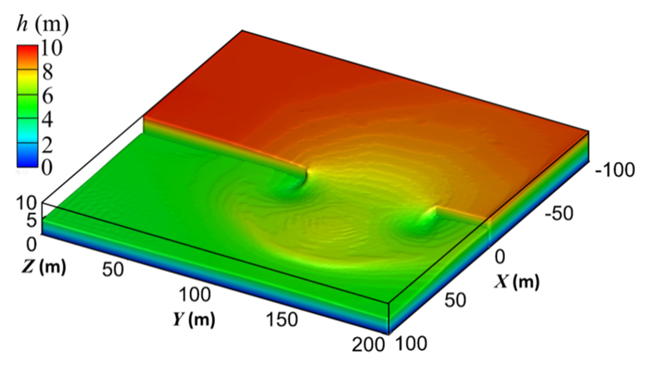
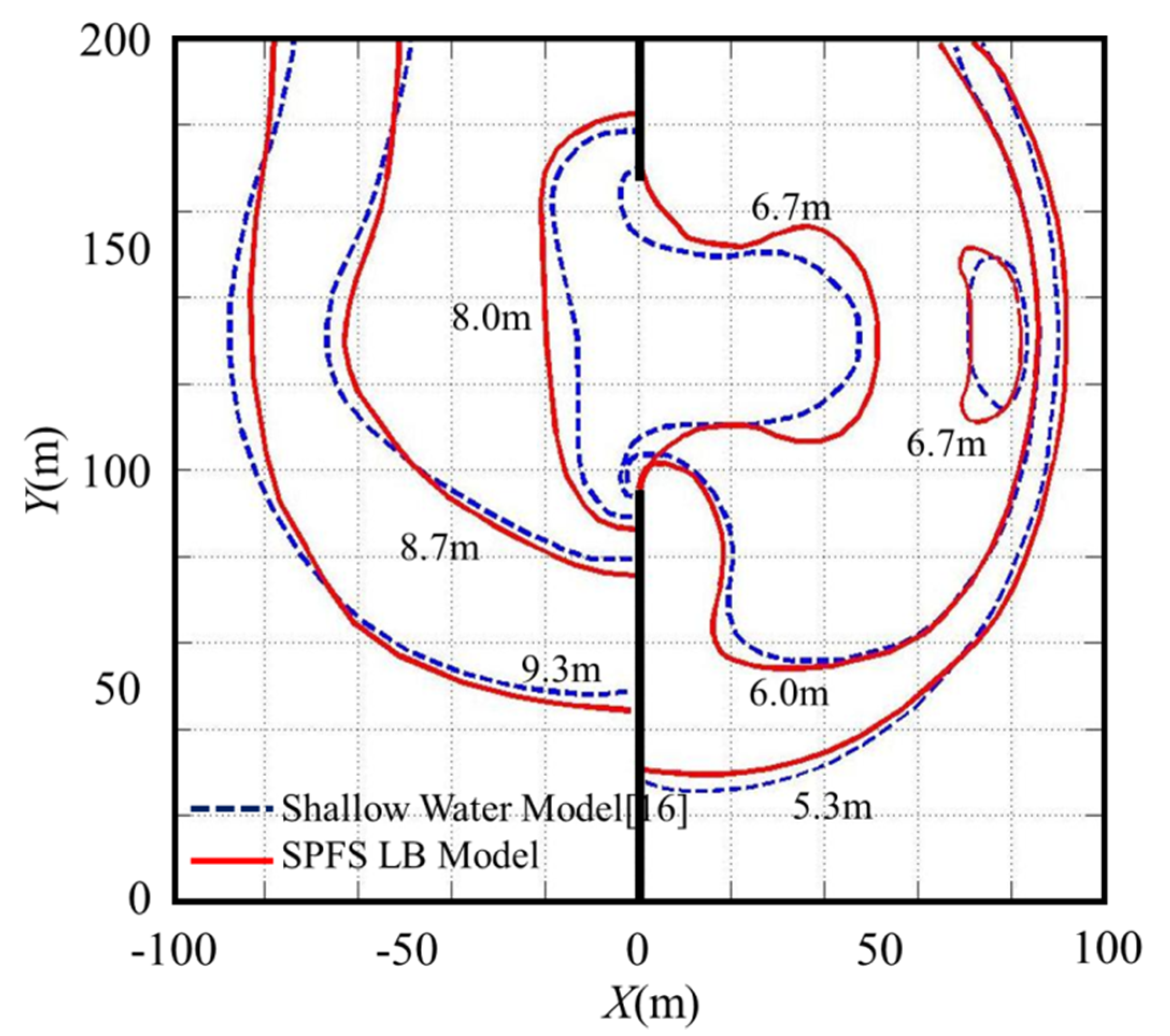
It is assumed that the upstream reservoir and downstream reservoir are both flat channels with a width of 200 m and a length of 100 m. The dam site is in the middle of the channel (X = 0 m), and the gap is located 95–170 m from the dam body (Y = 95–170 m, see Figure 4). At the beginning of the simulation, the upstream water depth is H = 10 m and downstream depth is h = 5 m.
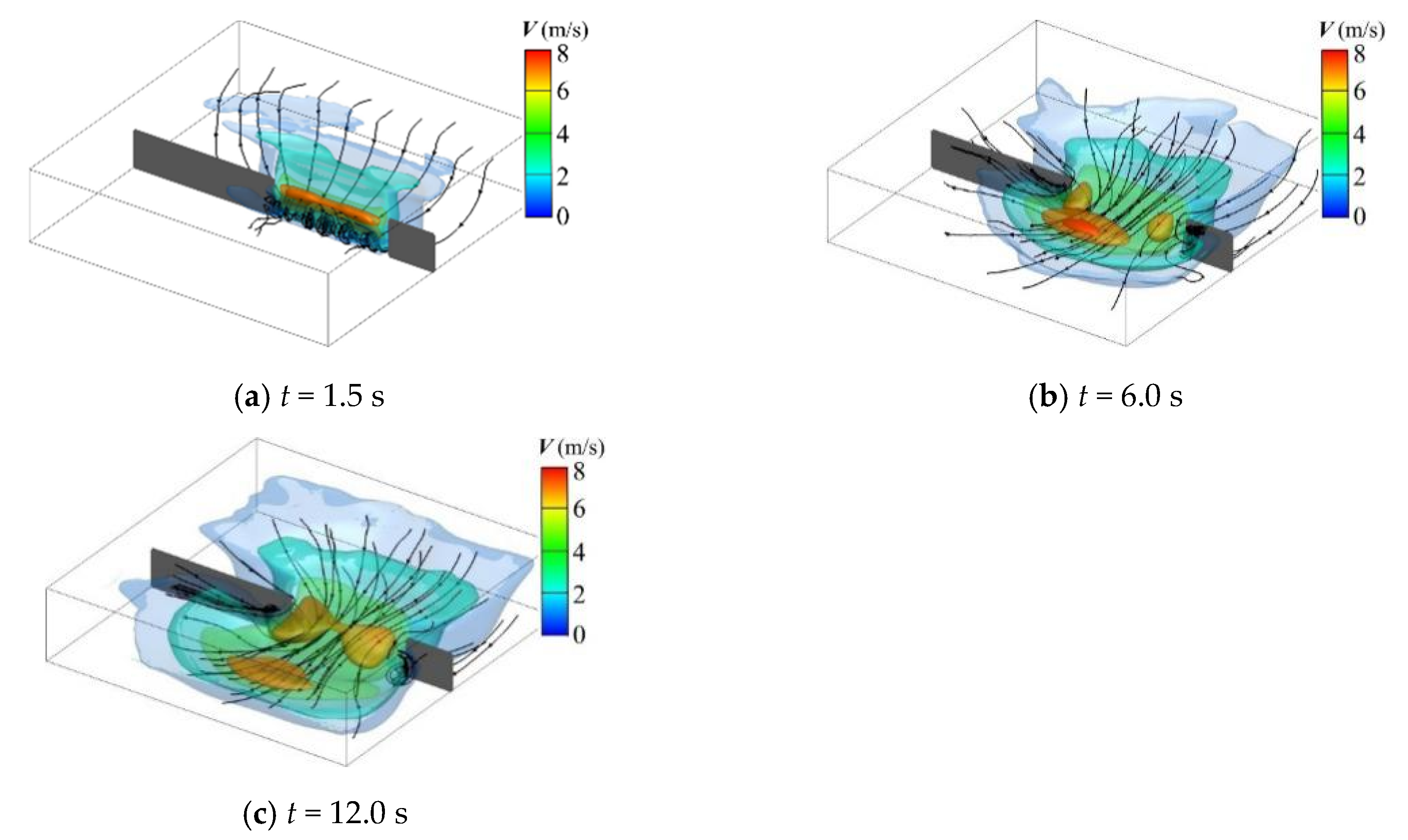
In this case, a 384 × 384 × 19 uniform lattice (Δx = 0.52 m) is conducted to the simulation. All the boundaries of the computational domain, including the dam body, are set as nonslip walls. The thickness of the dam body is double the lattice length (Δx). The water surface t = 10.1 s after dam failure is shown in Figure 3, and the velocity distribution and streamline are shown in Figure 4 at time t = 1.5 s, 6 s and 12 s.
When the partial dam break appears, there is a negative wave propagating to the upstream channel and a positive wave propagating to the downstream channel, and the wave propels in an arc shape. Upstream of the dam, the water around the dam flows towards the gap, and the water surface forms a “funnel” shape. The “funnel” shape enlarges and moves upstream as time goes by. At the downstream of the dam, the positive wave generates backflows around the dam and forms vertical-axis vortices on both sides of the dam gap. The above simulated results are consistent with the existing knowledge on partial dam-break flows [16,20]. The computed results of the SPFS-LB model and shallow water model are compared in Figure 5. It can be seen from Figure 5 that the wavefront position and wave profile of SPFS-LB model are approximately the same as the reference [16], which means that the model proposed in this paper can accurately capture the generation and development process of partial dam-break flow.
Besides of the horizontal wave profile, the SPFS-LB model can also be adopted to analyze the vertical flow structure of dam-break waves, as shown in Figure 4. Under the shearing caused by the falling water from upstream, a horizontal-axis vortex parallel to the dam body forms at the bottom of channel at the initial stage of the dam-break flow (see Figure 4a), and this vortex disappears until the stable and uniform flow state forms at the bottom of channel (see Figure 4b). After a few seconds, as the propagation and reflection of the positive wave, two vertical-axis vortices successively form on both sides of the dam gap (see Figure 4c).
3.3. Simulation of Dam-Break Flow over a Triangular Step
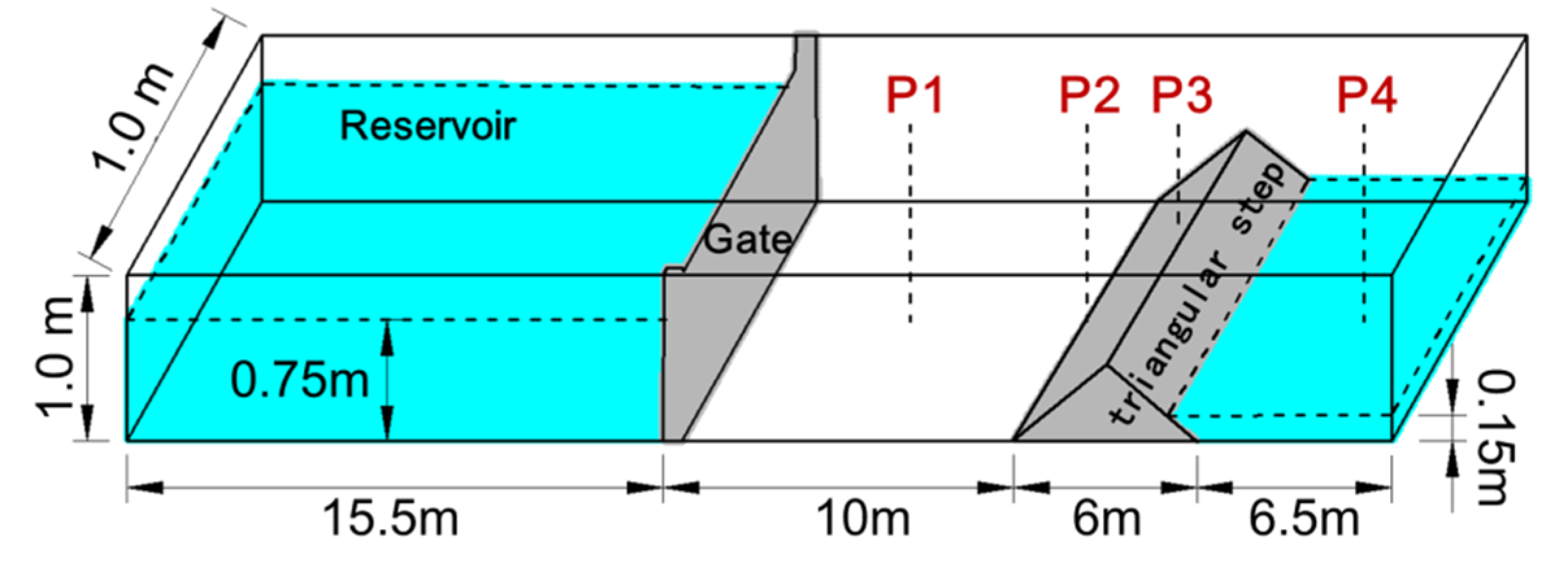
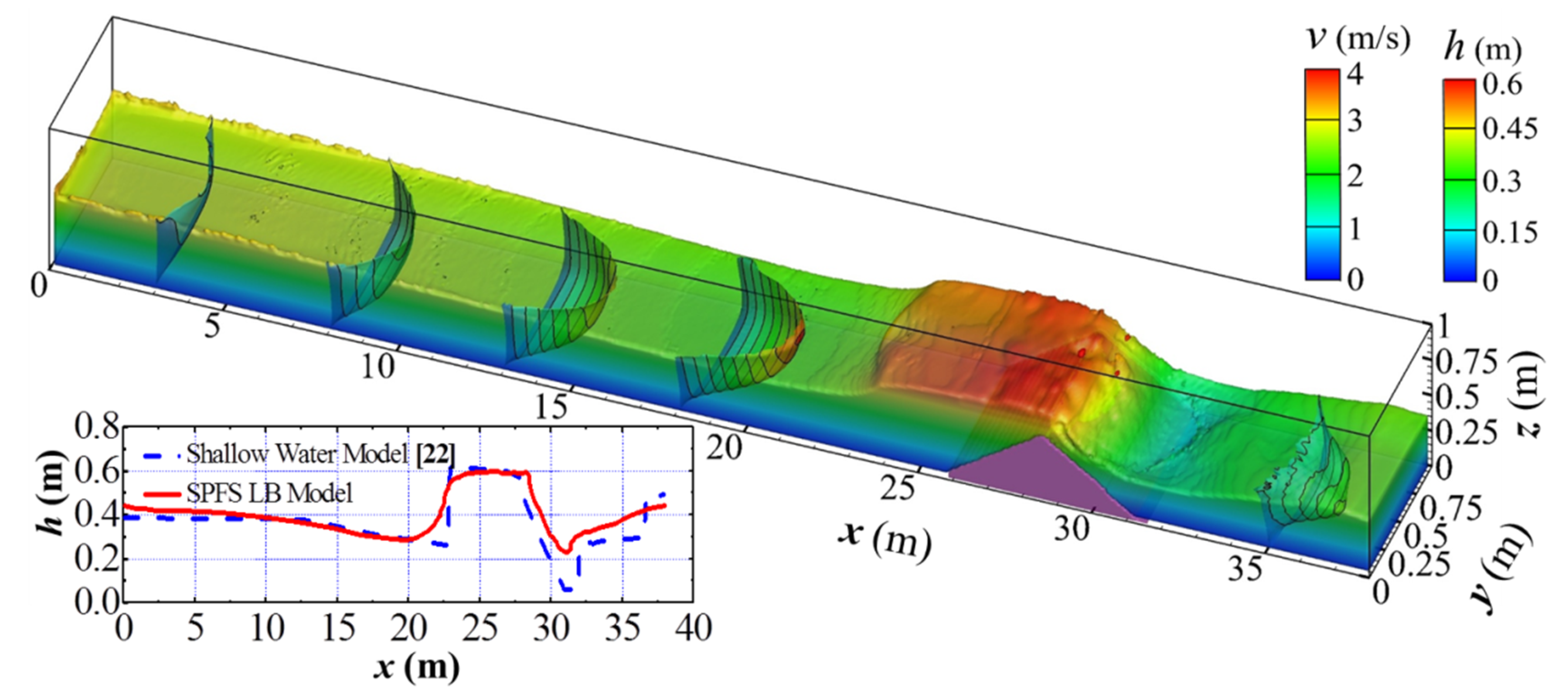
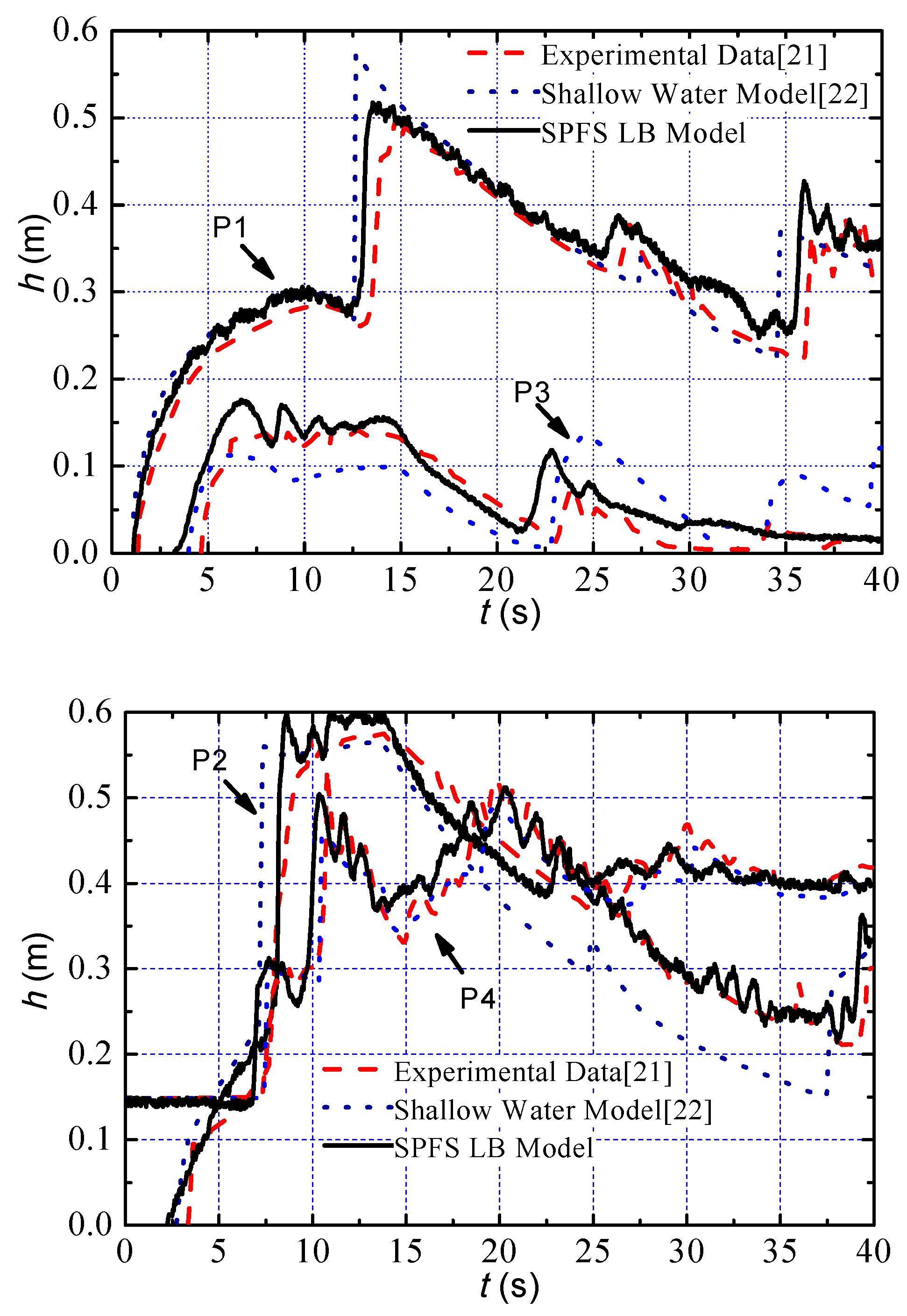
The experimental data of dam-break flow over a triangular step, tested by the European Union CADAM (the European Concerted Action on Dam-break Modeling) project [21], were used to validate the SPFS-LB model. This case includes various free-surface flow phenomena including overtopping flows, partial reflections, hydraulic jumps, hydraulic drops, and multiple wave interactions. As shown in Figure 6, the total length of the channel is 38 m, and the dam is 15.5 m away from the upstream boundary. A triangular step, with a length of 6.0 m and a height of 0.4 m, is placed 10 m downstream of the dam. The water depth at upstream of the dam is 0.75 m, and the water depth at downstream of the triangular step is 0.15 m. Four points to observe the evolutions of water depth are arranged along the central axis of the channel, and the distance away from the upstream dam is 4 m, 10 m, 13 m, and 20 m, respectively, which is the same as the experimental work in reference [21]. The simulation is performed on a 2304 × 61 × 61 uniform lattice (Δx = 0.016 m, number of lattice nodes: 8.57 million), and all boundaries in the model are set as nonslip walls. Figure 7 shows the water surface and flow field of the simulated dam break flow at t = 9.7 s, and the water surface is compared with the results obtained by shallow water method. See Figure 8 for comparison of the evolutions of water depth at four observation points between the present study and the references.
It can be seen from Figure 8 that the waves reach observing point P1 at time t = 1.2 s. During the evolution of dam-break waves, the velocity profile of flows forms a paraboloid shape. The dam-break waves reach P2 at t = 2.4 s and begin to climb the slope, and partially reflected waves propagate back to P1, which causes a disturbance of water surface at P1 (t = 4.8 s). After t = 4.1 s, the water flow rushes down quickly over the triangular step and forms rapid flow. The hydraulic jump appears at downstream of the step (X = 32–35 m) at this moment. Then, the waves caused by the hydraulic jump reach P4 at t = 7.1 s. The waves reflected from the triangular step or the right wall reaches P2, P4, and P1 at 7.9 s, 9.8 s, and 13.1 s successively, which makes the water depth abruptly go up to 0.60 m, 0.48 m, and 0.52 m. After t = 20.0 s, the water depths at the four observation points decrease with some fluctuations because the downstream boundary of the model is closed and oscillating flows appear in the channel.
In the present simulation, the fluctuated water depth at the observing points and the instantaneous water surface of dam-break wave at t = 9.7 s agree well with the experimental data [21] and the simulated result [22] respectively, which means the SPFS-LB model can analyze the fluctuations of the water surface induced by the progressive and reflected dam-break waves well. As for the histories of the water depth at the observing points during the evolution of dam-break waves, the simulated result is obviously superior to that of reference [22]. The reason is that the 2D shallow equation cannot simulate the vertical water flows effectively.
3.4. Simulation of Flood Discharge of an Arch Dam
3.4.1. Analysis of Flow Patterns
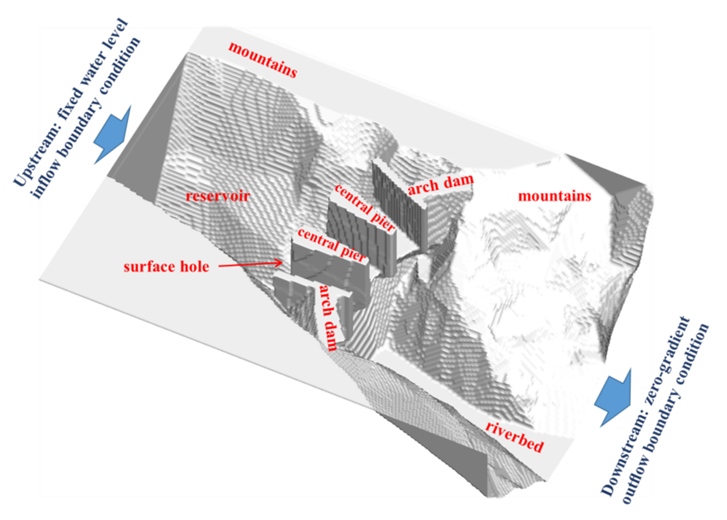
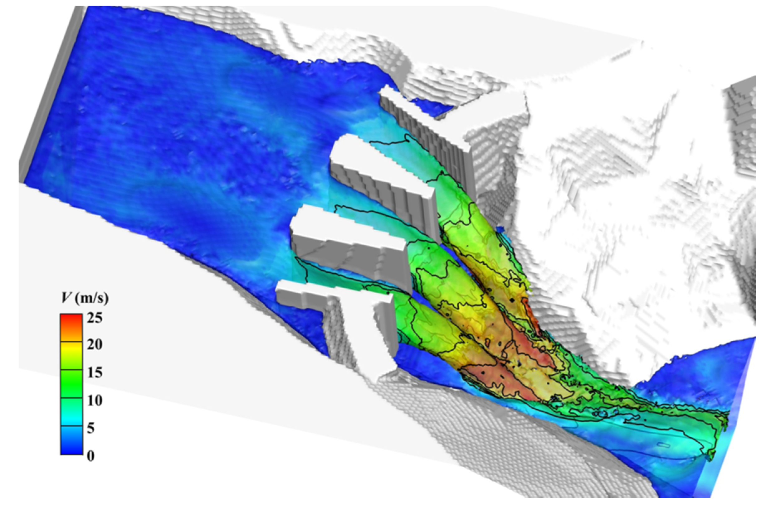
At last, the flood discharge of an arch dam is simulated. The outlet structures of the arc dam are three surface holes (10 m wide, 14.5 m high) on the dam crest. The bottom of the surface hole is made up of a practical weir (WES shape), of which the top and tail elevation are 442 m and 438 m, respectively. Among the surface holes, there are two central piers with variable width (upstream: 6.53 m, downstream: 2 m). A 384 × 512 × 192 uniform lattice is implemented for this computation. The present simulation analyzes flows within the spatial scale of 100 m × 133 m × 50 m (Δx = 0.2 6m, lattice node: 37.75 million), as seen in Figure 9. In the computational domain, the upstream boundary is set as a fixed water level inflow boundary condition, while the downstream boundary is set as a zero-gradient outflow boundary condition (for details, see reference [23]). Other boundaries, such as arc dam, riverbed, and mountains, are set as nonslip wall boundary conditions. See Figure 10 for the simulated surface velocity distribution, and Figure 11 for the liquid volume fraction of the vertical section.
According to the simulated results, after flowing through the surface holes of an arc dam, the water from the upstream reservoir freely falls into the downstream river channel and forms a tongue-shaped jet flow. The speed of the flow increases continuously during falling due to gravity. The discharge capacity of the two side holes is lower than that of the center hole under the influence of the reservoir banks, and the water trough formed from the center hole is thicker and larger. The water discharged from the surface holes collides with the water at the downstream of the arc dam, and the maximum local velocity of flow reaches approximately 25 m/s. The water in the downstream river channel rolls over strongly due to the impact of discharged water, and the water surface fluctuates randomly. The velocity of the plunging flow drastically decreases during the process of collision and rollover. As shown in Figure 10, the flow velocity of the mainstream reduces to 10 m/s 50 m downstream of the arc dam, which significantly relieves the scouring effect of the plunging flow. The flow phenomena indicates the good energy dissipation by the trajectory jet flows, and it can meet the project’s requirements for flood energy dissipation. This work has successfully simulated the impact, breaking down, and merging of high-speed flows, which reflects the strong 3-D features of flow structure during the flood discharge of surface holes.
The present work has simulated the flood discharge of the arc dam with upstream reservoir water levels of 445 m, 450 m and 455 m. See Table 1 for comparison of the discharge coefficients between the simulated results and those obtained by the empirical formula in reference [24]. Factors such as side shrinkage and upstream weir surface form are taken into consideration when the discharge coefficients are calculated by the empirical formula. It can be seen that the simulated discharge coefficient agrees well with the value of the empirical formula, with maximal relative error of 4.10%, which is sufficient for simulating engineering applications. This simulation shows that the SPFS-LB model can be used to simulate the 3-D large-scale free-surface flow problems in the field of hydraulic projects, so as to provide technological basis for the relevant engineering design.
3.4.2. Analysis of Lattice Sensitivity
To study the lattice sensitivity of the present scheme, the normalized parameters are fixed and the lattice of the simulation is refined gradually (192 × 256 × 96, 288 × 384 × 144 and 384 × 512 × 192 uniform lattices, respectively). The relative deviations for the discharge coefficients are shown in Table 2 with the reservoir water level fixed at H = 450 m.
It can be seen in Table 2 that the relative deviations for the discharge coefficients basically keep constant with the refinement of lattice, which means the simulated results would not significantly change with the increasing number of grid. This suggests that the results in Section 3.4 are obtained on a convergent grid.
4. Conclusions
The SPFS-LB model is coupled with the large-eddy simulation method in this paper, and the model successfully simulates several large-scale free surface flow problems in the field of hydraulic projects. Then, the simulations are implemented on GPU chips to improve the computational efficiency. The results indicate that the proposed method is efficient and accurate enough to study practical engineering flow problems.
Firstly, the conventional dam-break waves and dam-break flows over a triangular step are simulated. Good agreements between the simulated results and the reference data validate the accuracy of the present model in studying large-scale free surface flows. Then, as a first attempt at analyzing practical engineering flows, the flood discharge of an arch dam is simulated, and the discharge coefficient also agrees well with the empirical results. Finally, parallel computations of the present model based on GPU codes can make full use of the algorithm advantage of the LB method with low coupling degree, which improves the computing efficiency of the simulations by dozens of times.
In the future, fluid–structure interaction, thermal model, mass transfer, and other mathematical models will be added to the present method. The new coupling model will be implemented on GPU chips, so as to achieve accurate and efficient analysis of other engineering problems, such as landslide surge waves, thermal stratification, and pollution diffusion in large reservoirs.
Author Contributions
Methodology, Y.P.; Investigation, Y.P.; Resources, X.Z.; Funding acquisition, X.Z.; Software, W.D.; Supervision, W.D.; Validation, C.Z.; Writing—original draft, Y.P.; Writing—review&editing, S.Y.
Funding
This research was funded by [Natural Science Foundation Projrct of CQ CSTC] grant number [(KJQN201800712)].
Acknowledgments
The authors are grateful to the financial support from Agency for Science, Technology and Research of Singapore under Project No. 0421010018.
Conflicts of Interest
The authors declare no conflict of interest.
Appendix A. Parallel Computing of the SPFS-LB Model on a GPU
Appendix A.1. Technology of Parallel Computing on a GPU
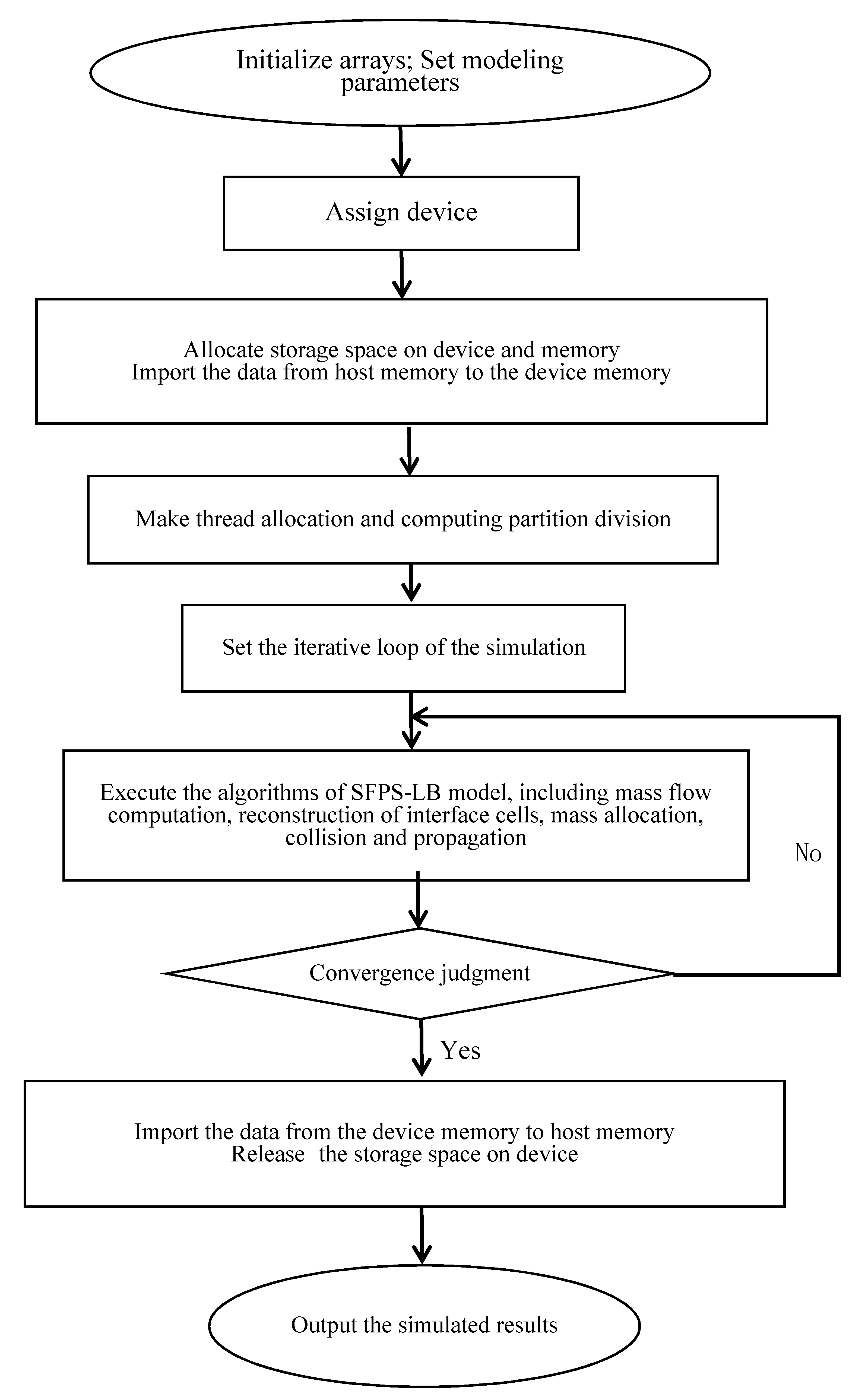
The implementation of the parallel computing in this work is based on general purpose GPU programming architecture of Compute Unified Device Architecture (CUDA) which is proposed by the nVidia Company. During the programming, rational resource allocation, proper task partitioning, and flexible boundary treatment shall be carried out according to the algorithm features of the SFPS-LB model to maximize the computing capacity of the GPU. A brief introduction to the parallel computing of the SFPS-LB model is as follows (see Figure A1 for program structure):
Figure A1.
Parallel program of the SPFS-LB model based on Compute Unified Device Architecture (CUDA).
Figure A1.
Parallel program of the SPFS-LB model based on Compute Unified Device Architecture (CUDA).

Appendix A.2. Analysis of Parallel Computing
The GPU parallel codes and CPU serial codes are used to compute the above flood discharge flows. The computations are based on different lattice densities, so as to obtain the speed-up ratio of parallel computing. The GPU parallel codes are carried out on the CUDA 7.5 platform, and the iterative computation of kernel functions is run on a single NVIDIA GeForce GTX Titan X graphics card. The read-in/output of computation files are assisted by Dell Precision 3620 workstation (Intel i7-6700k CPU). The CPU serial codes are implemented on VS2010 through C++, running on a Dell Precision 3620 workstation.
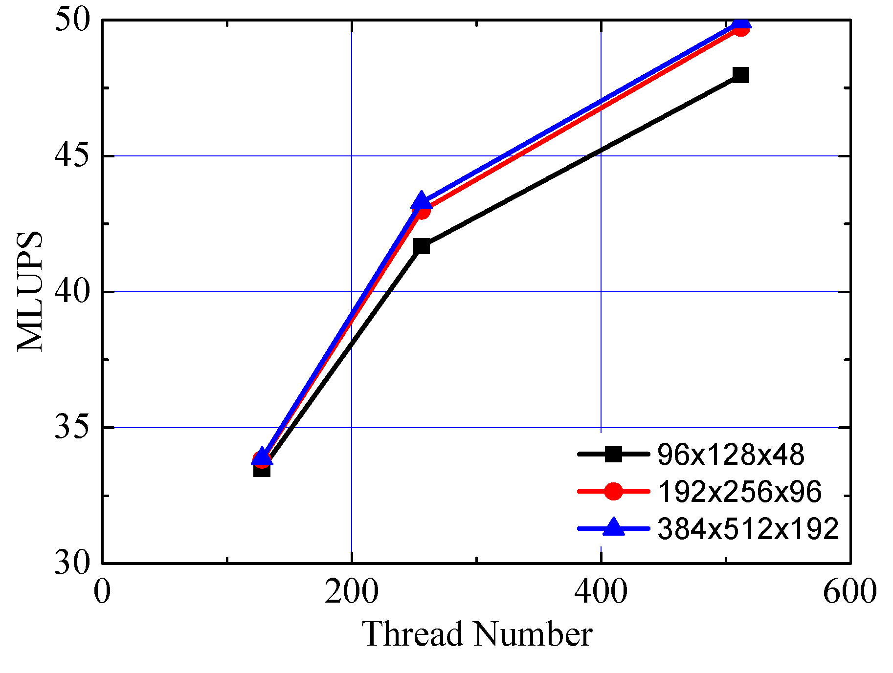
Table A1 gives the million lattice node updates per second (MLUPS) and the speed-up ratio for double-precision computation of GPU codes to CPU codes with three sets of lattices. The first column shows the computational lattices, and the header of the GPU column refers to the thread number specified by each thread block. In addition, the digits before and in brackets refer to MLUPS and speed-up ratio respectively. The MLUPS of GPU codes with different thread number is compared in Figure A2.

Table A1.
Million lattice node updates per second (MLUPS) and speedup of GPU and CPU.
| Lattice | GPU | CPU | ||
|---|---|---|---|---|
| 128 | 256 | 512 | MLUPS | |
| 96 × 128 × 48 | 41.19 (33.48) | 51.26 (41.67) | 59.00 (47.96) | 1.23 |
| 192 × 256 × 96 | 40.92 (33.82) | 52.00 (42.98) | 60.03 (49.61) | 1.21 |
| 384 × 512 × 192 | 41.31 (33.86) | 52.82 (43.30) | 60.92 (49.93) | 1.22 |
The MLUPS of GPU codes increases with the increasing thread number specified by thread blocks, which is determined by the hardware features of GTX Titan X graphics card and loading mode of CUDA instruction set. When all the warps in a thread block are suspended, stream processors can execute instructions from warps in the next thread block immediately. If the thread number in thread blocks for parallel computing increases, each stream processor can obtain more workload from active thread blocks. In other words, reasonable increase of thread number can hide the latency of stream processors effectively, so the computing efficiency is improved. When the thread number of blocks is sufficient, the high-efficiency shared memory channel and processor registers can be fully used to guarantee the computing efficiency. Therefore, if the thread number is rationally specified, compared with CPU codes, GPU codes can achieve a maximum speedup of approximately 50 times (see Table A1 and Figure A2). Specifically, for the simulation of 10 second flood discharge flows (lattice node: 37.75 million), the computation based on GPU codes will take 22.7 h, while computation based on CPU codes will take about 47 days. This also reflects the high efficiency of the SPFS-LB method computed by GPU codes.
Figure A2.
MLUPS of a GPU with different thread number.

References
- Heinrich, P. Nonlinear Water Waves Generated by Submarine and Aerial Landslides. J. Waterw. PortCoast. Ocean Eng. 1992, 118, 249–266. [Google Scholar] [CrossRef]
- Cai, F.; Cheng, Y.G.; Zhang, X.X. Method to guarantee accuracy of 3-D CFD simulation of water level in surge chamber. Wuhan Univ. J. (Eng. Sci. Ed.) 2016, 49, 390–396. (In Chinese) [Google Scholar]
- Machiels, O.; Pirotton, M.; Pierre, A.; Dewals, B.; Erpicum, S. Experimental parametric study and design of Piano Key Weirs. J. Hydraul. Res. 2014, 52, 326–335. [Google Scholar] [CrossRef]
- Zhang, X.H.; Long, W.F.; Lei, X.Z.; Zhang, X.W.; Xie, H.P.; Wang, J.P. Numerical simulation of flood inundation processes by 2D shallow water equations. Front. Archit. Civ. Eng. China 2007, 1, 107–113. [Google Scholar] [CrossRef]
- Pan, J.F.; Feng, M.J.; Zheng, B.M.; Ming, T. Two-dimensional numerical simulation on spur dike circumfluence and local scour hole. J. Sichuan Univ. (Eng. Sci. Ed.) 2005, 37, 15–18. (In Chinese) [Google Scholar]
- Hieu, P.D.; Katsutoshi, T.; Ca, V.T. Numerical simulation of breaking waves using a two-phase flow model. Appl. Math. Model. 2004, 28, 983–1005. [Google Scholar] [CrossRef]
- Hirt, C.; Nichols, B. Volume of fluid (VOF) method for the dynamics of free boundaries. J. Comput. Phys. 1981, 39, 201–225. [Google Scholar] [CrossRef]
- Sussman, M.; Smereka, P.; Osher, S. A Level Set Approach for Computing Solutions to Incompressible Two-Phase Flow. J. Comput. Phys. 1994, 114, 146–159. [Google Scholar] [CrossRef]
- Shen, J.; Yang, X. A Phase-Field Model and Its Numerical Approximation for Two-Phase Incompressible Flows with Different Densities and Viscosities. Siam J. Sci. Comput. 2010, 32, 1159–1179. [Google Scholar] [CrossRef]
- Dai, M.; Schmidt, D.P. Adaptive tetrahedral meshing in free-surface flow. J. Comput. Phys. 2005, 208, 228–252. [Google Scholar] [CrossRef]
- Harlow, F.H.; Welch, J.E. Numerical calculation of time-dependent viscous incompressible flow of fluid with free surface. Phys. Fluids 1965, 8, 2182–2189. [Google Scholar] [CrossRef]
- Kelly, D.M.; Chen, Q.; Zang, J. PICIN: A Particle-in-Cell Solver for Incompressible Free Surface Flows with Two-Way Fluid-Solid Coupling. Siam J. Sci. Comput. 2015, 37, B403–B424. [Google Scholar] [CrossRef] [Green Version]
- Thürey, N. A Single-Phase Free-Surface Lattice Boltzmann Method. Master’s Thesis, Friedrich-Alexander-Universität of Erlangen-Nürnberg, Erlangen, Germany, 2003. [Google Scholar]
- Körner, C.; Thies, M.; Hofmann, T.; Thürey, N.; Rüde, U. Lattice Boltzmann Model for Free Surface Flow for Modeling Foaming. J. Stat. Phys. 2005, 121, 179–196. [Google Scholar] [CrossRef]
- Aidun, C.K.; Clausen, J.R. Lattice-Boltzmann Method for Complex Flows. Annu. Rev. Fluid Mech. 2010, 42, 439–472. [Google Scholar] [CrossRef]
- Zhang, C.Z.; Cheng, Y.G.; Li, Y.C. Lattice boltzmann model for two-dimensional shallow water flows realizing parallel computing on GPU. J. Hydrodyn. Ser. A 2011, 26, 194–200. (In Chinese) [Google Scholar]
- Lallemand, P.; Luo, L.-S. Theory of the lattice Boltzmann method: Dispersion, dissipation, isotropy, Galilean invariance, and stability. Phys. Rev. E 2000, 61, 6546–6562. [Google Scholar] [CrossRef] [Green Version]
- Manfred, K.; Jonas, T.; Luo, L.S. Large eddy simulation with a multiple-relaxation-time LBE model. Int. J. Mod. Phys. B 2008, 17, 33–39. [Google Scholar] [CrossRef]
- Stoker, J.J.; Lindsay, R.B. Water Waves. Phys. Today 1958, 11, 28–30. [Google Scholar] [CrossRef]
- Liu, H.; Zhou, J.G.; Burrows, R. Lattice Boltzmann simulations of the transient shallow water flows. Adv. Water Resour. 2010, 33, 387–396. [Google Scholar] [CrossRef]
- Miller, S.; Chaudhry, M.H. Dam-break Flows in Curved Channel. J. Hydraul. Eng. 1989, 115, 1465–1478. [Google Scholar] [CrossRef]
- Zhou, J.G.; Causon, D.M.; Mingham, C.G.; Ingram, D.M. Numerical Prediction of Dam-Break Flows in General Geometries with Complex Bed Topography. J. Hydraul. Eng. 2004, 130, 332–340. [Google Scholar] [CrossRef]
- Tang, B.; Li, J.; Wang, T. Single-phase lattice Boltzmann model for free-surface flow. J. Tsinghua Univ. 2008, 48, 2017–2020. (In Chinese) [Google Scholar]
- Zhao, X.; Zhang, X.Y.; Zhao, M.D. Hydraulics; China Electric Power Press: Beijing, China, 2009. [Google Scholar]
Figure 1.
Cell types of SPFS-LB method.

Figure 2.
Water surface profile of a 1-D dam-break wave (60 s after dam failure), (a) h = 1.75 m, (b) h = 5 m.
Figure 2.
Water surface profile of a 1-D dam-break wave (60 s after dam failure), (a) h = 1.75 m, (b) h = 5 m.

Figure 3.
Water surface of the partial dam-break wave at t = 10.1 s.

Figure 4.
Velocity of partial dam-break flows, (a) t = 1.5 s, (b) t = 6.0 s, (c) t = 12.0 s.

Figure 5.
Contour of partial dam-break flows at t = 10.1 s.

Figure 6.
Sketch of dam-break flow over a triangular step.

Figure 7.
Water surface and velocity profile of dam-break flows at t = 9.7 s.

Figure 8.
Water surface time series of measuring point.

Figure 9.
The geometry of flood discharge of an arch dam.

Figure 10.
Water surface and velocity of flood discharge of an arch dam (reservoir water level: 450 m).
Figure 10.
Water surface and velocity of flood discharge of an arch dam (reservoir water level: 450 m).

Figure 11.
Liquid volume fraction of the vertical section (reservoir water level: 450 m).

Table 1.
Comparison of the discharge coefficients between the simulated results and the empirical formula results.
Table 1.
Comparison of the discharge coefficients between the simulated results and the empirical formula results.
| Reservoir Water Level (m) | 445 | 450 | 455 | |
|---|---|---|---|---|
| Empirical formula results [24] | Side contraction coefficients | 0.958 | 0.929 | 0.889 |
| H/Hd | 0.307 | 0.820 | 1.332 | |
| Discharge coefficients | 0.419 | 0.487 | 0.530 | |
| Simulated results | Discharge coefficients | 0.402 | 0.477 | 0.543 |
| Relative error (%) | 4.1 | 2.1 | 2.6 | |
Note: H = reservoir water level—442 m, it refers to weir head; Hd refers to the design head, which is taken as 9.76 m according to the design data of the arc dam.
Table 2.
Relative error between the simulated results and empirical formula results with different lattices.
Table 2.
Relative error between the simulated results and empirical formula results with different lattices.
| Lattice | Δx | Discharge Coefficients | Relative Deviation | |
|---|---|---|---|---|
| Simulated Results | Empirical Formula Results [24] | |||
| 96 × 128 × 48 | 0.52 m | 0.470 | 0.487 | 3.5% |
| 192 × 256 × 96 | 0.39 m | 0.475 | 0.487 | 2.4% |
| 384 × 512 × 192 | 0.26 m | 0.477 | 0.487 | 2.1% |
© 2019 by the authors. Licensee MDPI, Basel, Switzerland. This article is an open access article distributed under the terms and conditions of the Creative Commons Attribution (CC BY) license (http://creativecommons.org/licenses/by/4.0/).
Share and Cite
MDPI and ACS Style
Peng, Y.; Diao, W.; Zhang, X.; Zhang, C.; Yang, S. Three-Dimensional Numerical Method for Simulating Large-Scale Free Water Surface by Massive Parallel Computing on a GPU. Water 2019, 11, 2121. https://doi.org/10.3390/w11102121
AMA Style
Peng Y, Diao W, Zhang X, Zhang C, Yang S. Three-Dimensional Numerical Method for Simulating Large-Scale Free Water Surface by Massive Parallel Computing on a GPU. Water. 2019; 11(10):2121. https://doi.org/10.3390/w11102121
Chicago/Turabian StylePeng, Yongqin, Wei Diao, Xujin Zhang, Chunze Zhang, and Shuqing Yang. 2019. "Three-Dimensional Numerical Method for Simulating Large-Scale Free Water Surface by Massive Parallel Computing on a GPU" Water 11, no. 10: 2121. https://doi.org/10.3390/w11102121
Note that from the first issue of 2016, this journal uses article numbers instead of page numbers. See further details here.