Innovative Variance Corrected Sen’s Trend Test on Persistent Hydrometeorological Data

Abstract

Trend detection in observations helps one to identify anthropogenic forces on natural hydrological and climatic systems. Hydrometeorological data are often persistent over time that deviates from the assumption of independence used by many statistical methods. A recently proposed Sen’s trend test claimed to be free of this problem and thereby received widespread attention. However, both theoretical derivation and stochastic simulation of the current study implies that persistence inflates the trend significance, leading to false trends. To tackle this problem, we incorporate the feature of persistence into the variance of the trend test statistic, whereby an innovative variance-corrected Sen’s trend test is developed. Two theoretical variances of the trend test statistic are newly derived to account for short-term and long-term persistent behavior. The original variance for independent data is also corrected because of its negative bias. A stepwise procedure, including steps to specify the underlying persistent behavior and to test trend with new statistic, is outlined for performing the new test on factual data. Variance-corrected Sen’s trend test can effectively restore the inflated trend significance back to its nominal state. This study may call for the reassessment of published results of the original Sen’s trend test on data with persistence.

1. Introduction

Concerns are growing that hydrological systems have undergone substantial and unprecedented changes during the Anthropocene era. The IPCC’s reports highlighted the potential impacts and associated risks of global warming on natural and human systems, among which freshwater-related responses and risks were elaborated [1]. In general, renewable water resources are projected to decline in many dry subtropical regions. Approximately 7% of the global population would suffer from a severe reduction in renewable water resources with a 1 °C rise in global mean temperature [2]. Global warming research has motivated the widespread application of statistical change analysis in observed time series of hydrometeorological variables [3,4,5,6,7]. Trend detection is one branch of change detection methods, focusing on gradual changes that have far-reaching effects on the effectiveness of current water management policies. The presence of significant trends would entail a movement toward attributing causative effects and quantitative assessment of future evolution. Both the knowledge of past and potential changes could be incorporated into designing adaptation strategies to minimize impact and manage risk.

A comprehensive trend detection study commonly involves graphical and statistical analysis on trends throughout the observed hydrometeorological series. Graphical trend analysis allows an exploratory inspection of the available data and suggests qualitative information about the trend characteristics. For example, the rescaled adjusted partial sums (RAPS) tools can visualize small but systematic trends over time that are often hidden by internal variability of the data [8,9]. Statistical trend analysis quantifies the significance of trends in order to confirm the existence (or nonexistence) of trends detected by visual inspection. Most commonly used statistical techniques are Mann–Kendall test, Spearman Rho test, and linear regression test.

Recently, an innovative trend detection method, introduced by Sen [10,11,12], has got graphical and statistical analyses together. The graphical part of the method, Sen’s trend plot, was given the best technical note award by the American Society of Civil Engineers in 2014. Sen’s trend plot offers two major merits. First, it allows one to visually identify sub-trends in low, medium, and high clusters. The information is of practical importance for engineers to avoid missing significant hidden trends in extreme events such as high floods or severe droughts. Second, Sen’s trend plot can highlight trends even in short, skew distributed and persistent data. For these benefits, Sen’s trend plot has been widely embraced by the hydrological community and it was broadly applied to investigate trends in several hydrometeorological observations, such as in studies on precipitation [13,14], streamflow [15,16], air temperature [17], pan evaporation [18], solar radiation [19], water quality [20], and drought indexes [21,22].

The statistical part of the method, Sen’s trend test, was also claimed to be free of any assumptions, especially that of serial independence [11]. However, Sen’s trend test was built based on original data directly, and hence it cannot naturally remove interference by data persistence. The effect of persistence on Sen’s trend test still requires firm investigations via theoretical analysis and extensive simulation studies. This persistence, also called “serial dependence,” has been recognized as an inherent component of many natural, economic, and even medical data [23]. A persistent stochastic process exhibits enhanced variability at large time scales, as evidenced by the tendency in time series for high or low values to cluster together in many groups. This behavior came to be known as Hurst phenomenon. It is a manifestation of frequent and irregular fluctuations of climatic and hydrological processes on several scales. The emergence of persistence may produce some intense local slopes, which might be falsely identified as deterministic trends but actually are only segments of large scale random fluctuations. This is the fundamental impetus for developing appropriate statistical tests to accurately discriminate between real deterministic trends and natural persistent processes.

Among several efforts to account for persistence in trend significance tests, two techniques, namely data whitening and variance correction of the test statistic, play the dominant roles. The former renders the persistent data into a serially independent counterpart, by either removing autocorrelation or adding white noise [24,25]. The latter adapts the original trend test to persistent data via explicitly incorporating the persistence into the variance of the test statistic [26,27]. The intriguing property of the variance correction approach is that the influence of persistence on the trend test is transparent to users with grounded theoretical expressions. Additionally, it avoids artificially dismantling original data that are subject to the mutual effect of trends and persistence. For these reasons, the variance correction approach has become an active option to acclimatize trend tests to real world observations exhibiting persistent behavior. However, no literature has attached the variance of Sen’s trend test statistic to persistent data.

The main purpose of this study is to develop an innovative variance-corrected Sen’s trend test in which exact expressions for the variance of the trend test statistic under the persistence assumption are given. Our study begins by analyzing the original expression of variance proposed by Sen [11]. Interestingly, the original variance is substantially biased even in the absence of persistence, because of an error in its derivation. The theoretical variances for both serially independent and dependent data are newly derived. Based on this finding, we suggest a stepwise procedure for the implementation of a new test using actual data.

Simulation experiments and factual data applications are then carried out to evaluate and discuss the effectiveness of variance correction on mitigating the side effects of persistence on trend detection.

2. Sen’s Trend Detection Method

2.1. Sen’s Trend Plot

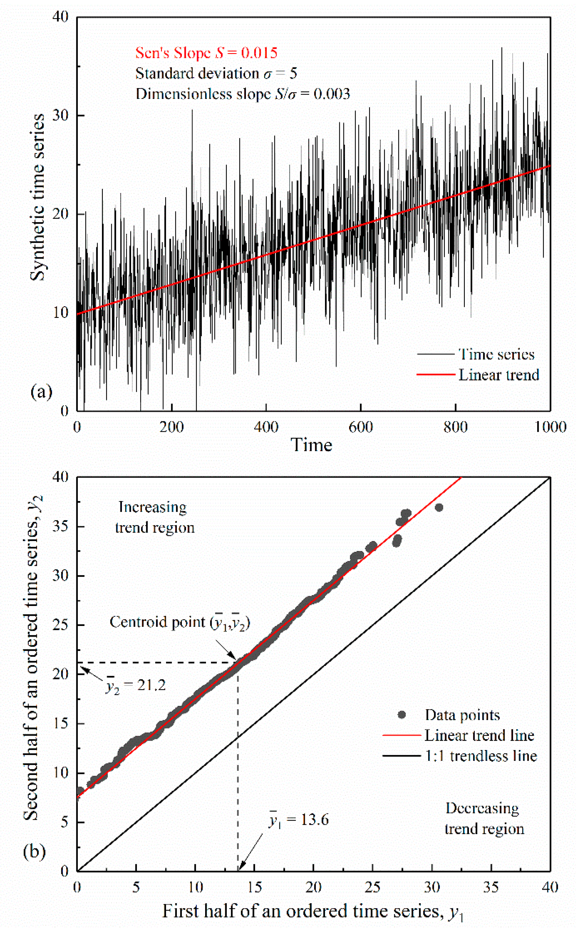
Sen’s method of trend detection proposes an innovative trend plot for the visual inspection of possible trends, including a quantitative assessment of trend slope and its statistical significance. In the preparation of the trend plot (Figure 1), the first step is to divide the given hydrometeorological time series into two equal halves and separately sort them in ascending order. The former half series is then placed on the horizontal axis and the latter half on the vertical axis of the Cartesian coordinate system. Finally, the scatter graph is rendered with the same scale on both axes and a 1:1 (45°) straight line is drawn. A monotonic upward (downward) trend clearly shows up when the scatter points wholly fall above (below) the 1:1 straight line. Nonmonotonic sub-trends are identified if the scatter points partially appear in the upper and lower triangular areas of the 1:1 straight line. If all the scatter points collect around the 1:1 straight line, the time series is nearly free of trend.

A linear trend, as a special pattern of monotonic trend, is widely employed to approximate a gradual change of a hydrometeorological time series having a constant change rate. It appears along a straight line parallel to the 1:1 line in the trend plot. The vertical distance between this “linear trend line” and the 1:1 line indicates the magnitude of the trend slope. There are alternative ways to determine the slope of the linear trend. The simplest way is to find the arithmetic average of the two half sub-series, which is the centroid of the linear trend line. The slope estimate of the linear trend $S$ is then formulated as:

$$S=\frac{2\left({\overline{y}}_2-{\overline{y}}_1\right)}{n}$$

(1)

where ${\overline{y}}_1$ and ${\overline{y}}_2$ are the means of the first and second half, respectively, and $n$ is the total series length.

Figure 1 illustrates the application of the trend plot for a synthetic time series, which was generated according to a Normally distributed white noise process with mean $\mu =10$, standard deviation $\sigma =5$, and length $n=1000$. A linear trend component with slope $S=0.015$ was superimposed onto the simulated series. In the corresponding trend plot (Figure 1b), most data points fall on the linear trend line. Equation (1) yields $S=0.0152$, which is very close to the embedded slope.

2.2. Sen’s Trend Test

A trend significance test is constructed by considering the statistical confidence interval of the slope estimator $S$. If the trend slope estimator $S$ is sufficiently far from zero, then we can deduce an existence of trends. Trend significance can be assessed by performing hypothesis tests on the slope estimator. The null hypothesis $H_0$ of the trend test is that the process underlying the observed series is trendless if $S$ remains below a confidence limit at a pre-assigned significance level. Alternatively, $H_0$ is rejected and the detected trend is statistically significant. Under the null hypothesis, with the basic assumption that the data are independent and identically distributed, Sen [11] provided the mean and variance of the slope estimator as:

$$E\left(S\right)=\frac{2}{n}\left[E\left({\overline{y}}_2\right)-E\left({\overline{y}}_1\right)\right]=0$$

(2)

$$V_0\left(S\right)=\frac{8}{n^2}{\sigma }_{{\overline{y}}_1}{\sigma }_{{\overline{y}}_2}\left(1-{\rho }_{{\overline{y}}_1{\overline{y}}_2}\right)=\frac{8}{n^2}\frac{{\sigma }^2}{n}\left(1-{\rho }_{{\overline{y}}_1{\overline{y}}_2}\right)$$

(3)

where $E\left({\overline{y}}_1\right)$ and $E\left({\overline{y}}_2\right)$ are the expectations of the mean estimator of the first and second half-time series, respectively, ${\sigma }_{{\overline{y}}_1}$ and ${\sigma }_{{\overline{y}}_2}$ are the standard deviations, and ${\rho }_{{\overline{y}}_1{\overline{y}}_2}$ is the cross correlation, $\sigma$ is the standard deviation of the entire time series.

Since all the odd-order moments of the slope estimator are equal to zero, the slope estimator approximately obeys the Normal distribution with a zero mean. For assessing the significance of the trend slope, the standardized $S$ statistic $Z_S=S/\sqrt{V_0\left(S\right)}$ is compared with the standard Normal variates $Z_{\alpha /2}$ and $Z_{1-\alpha /2}$ at a desired significance level $\alpha$, where $Z_{\alpha /2}$ and $Z_{1-\alpha /2}$ are the $\alpha /2$ and $1-\alpha /2$ quantiles of the standard Normal distribution $N\left(0,1\right)$. Significant upward (downward) trends are identified if $Z_S>Z_{1-\alpha /2}$ ($Z_S<Z_{\alpha /2}$).

Herein, we discuss the problems about the form of trend slope variance $V_0\left(S\right)$ derived by Sen [11]. In the case of the null hypothesis of no trend, the two half sub-series represent one identical population, which implies $E\left({\overline{y}}_1\right)=E\left({\overline{y}}_2\right)$ and hence $E\left(S\right)=0$. Likewise, ${\sigma }_{{\overline{y}}_1}={\sigma }_{{\overline{y}}_2}=\sqrt{2}\sigma /\sqrt{n}$ which is the standard deviation of the mean estimator of a sub-series with length $n/2$. However, Sen [11] took the form of ${\sigma }_{{\overline{y}}_1}$ and ${\sigma }_{{\overline{y}}_2}$ as $\sigma /\sqrt{n}$ by mistake. Additionally, this classical relationship ${\sigma }_{{\overline{y}}_1}={\sigma }_{{\overline{y}}_2}=\sqrt{2}\sigma /\sqrt{n}$ is only valid for independent and identically distributed data. Sen [11] did not mention the use of assumption of independence explicitly but introduced it in the derivation of the trend test statistic unconsciously.

Another mistake is related to the fact that independent data are characterized by zero cross correlation among any two different time points, and therefore ${\rho }_{{\overline{y}}_1{\overline{y}}_2}=0$. The computation of cross correlation between the two sorted half-time series, as suggested by Sen [11], is theoretically unnecessary. After correcting the two mistakes that have been explained, the variance of the slope estimator has the following expression:

$$V_0\left(S\right)=\frac{16{\sigma }^2}{n^3}$$

(4)

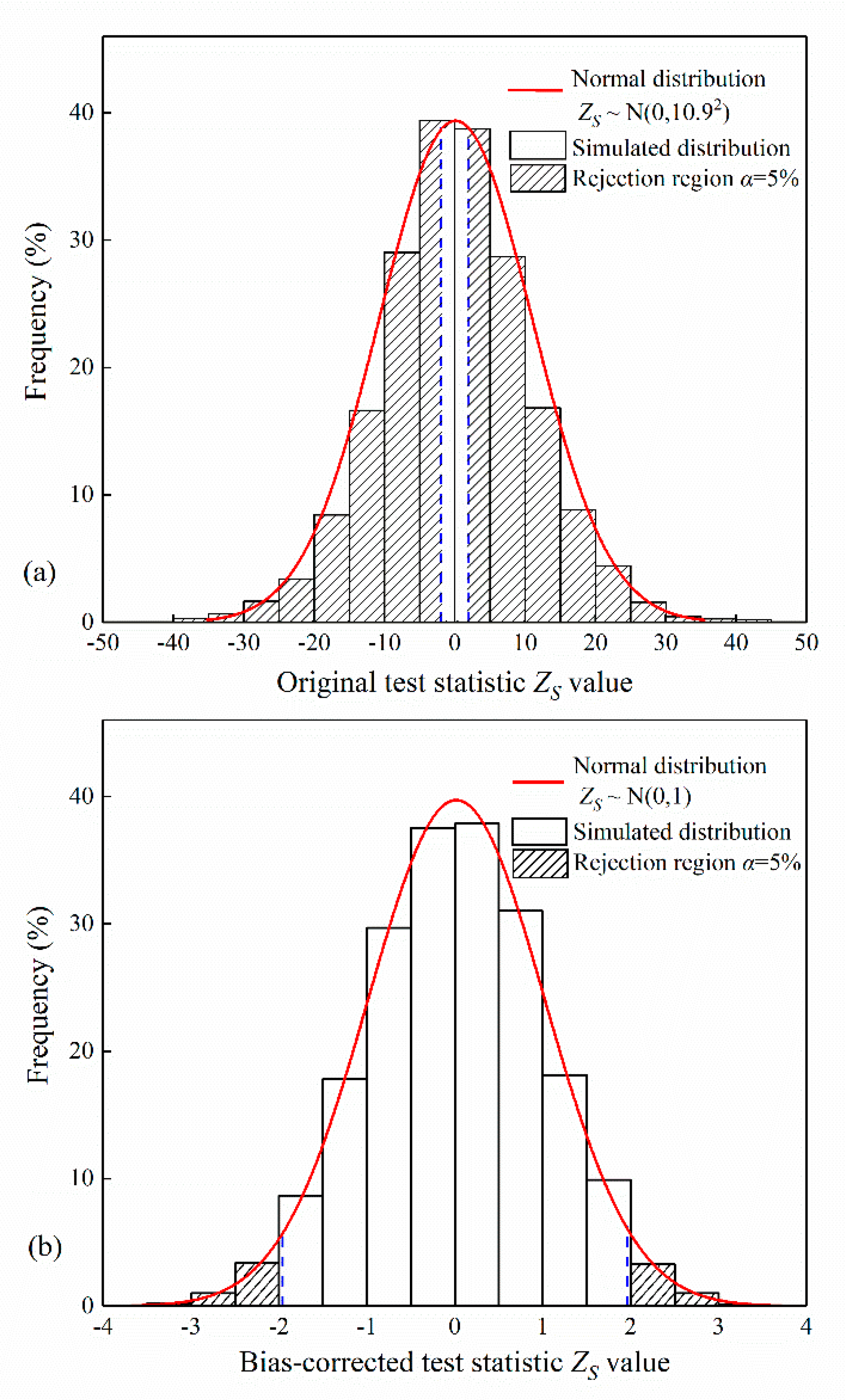
Figure 2 depicts the distribution histograms of the test statistic $Z_S$, using the original variance (Equation (3)) and the bias-corrected variance (Equation (4)), respectively, from 10,000 synthetic trendless independent data of length 100, with a Normal probability density function. The Normal distribution gives a satisfactory approximation to the distribution of $Z_S$. However, when using the original variance (Equation (3)), the distribution of $Z_S$ is too wide to preserve an expectable rejection ratio that should be equal to the significance level, as illuminated by Figure 2a. Such a high rejection ratio will result in many false indications of significant trends and lead to a spurious statement that the Sen’s trend test is much more powerful than other tests. After bias correction, the upper and lower tails of $Z_S$ still align with the Normal curve and further provide a proper rejection ratio (see Figure 2b). In the following analysis, the usefulness of the original Sen’s trend test was evaluated using the bias-corrected variance in Equation (4).

3. The Influence of Persistence on the Original Sen’s Trend Test

3.1. Persistence in Hydrometeorological Data

The original Sen’s trend test is tailored to independent data as mentioned above. Hydrometeorological data, on the other hand, are often time dependent and characterized by nonzero autocorrelation beyond the first lag. Two stochastic models that have been widely applied to describe natural processes were considered here to illustrate the effect of persistence on the original Sen’s trend test. The first model is the lag-one autoregressive model, namely AR(1), which is characterized by an exponentially decaying autocorrelation function. The autocorrelation of an aggregated AR(1) process drops down to zero for large time scales; hence, AR(1) is commonly used to simulate short-term persistent processes. The autocorrelation function of an aggregated AR(1) process is given by (e.g., [28]):

$${\rho }_j^{\left(k\right)}=\{\begin{array}{l}\begin{array}{cc}\frac{\rho {\left(1-{\rho }^k\right)}^2}{k\left(1-{\rho }^2\right)-2\rho \left(1-{\rho }^k\right)};& \left|j\right|=1\end{array}\\ \begin{array}{ccc}{\rho }_1^{\left(k\right)}{\rho }^{k\left|j-1\right|};& & \left|j\right|>1\end{array}\end{array}$$

(5)

where, $\rho$ is the lag-one autocorrelation coefficient at the basic time scale (e.g., one year), $k$ is the time scale of interest (e.g., 5 or 10 years), and $j$ denotes the time lag. Taking an annual series ($k=1$) as an example, the autocorrelation becomes a quite simple and familiar expression:

$${\rho }_j=\{\begin{array}{l}\begin{array}{cc}\rho ;& \left|j\right|=1\end{array}\\ \begin{array}{cc}{\rho }^{\left|j\right|},& \left|j\right|>1\end{array}\end{array}$$

(6)

Likewise, the variances of an aggregated AR(1) process are also related to the time scale of aggregation (i.e., $k$). The variance of the process at scale $k$ is given by:

$${\left({\sigma }^2\right)}^{\left(k\right)}={\sigma }^2\frac{k\left(1-{\rho }^2\right)-2\rho \left(1-{\rho }^k\right)}{{\left(1-\rho \right)}^2}$$

(7)

where ${\sigma }^2$ is used to abbreviate the variance of the process at the basic time scale $k=1$, i.e., (${\sigma }^2\equiv {\left({\sigma }^2\right)}^{\left(1\right)}$). Also $\rho$ denotes the lag-one correlation coefficient at $k=1$.

For a large value of $k$, Koutsoyiannis [28] simplified the expression of Equation (7) as:

$${\left({\sigma }^2\right)}^{\left(k\right)}=k\frac{\left(1+\rho \right)}{\left(1-\rho \right)}{\sigma }^2$$

(8)

The second model is Fractional Gaussian Noise (FGN), also known as the simple scaling stochastic process [28,29,30,31,32], which has a slowly-decaying autocorrelation function and is classified as a long-term persistent model. The FGN model is often more consistent with hydrometeorological reality than the classical AR(1) model, primarily because of its capability to reproduce natural random fluctuations on multiple time scales [33]. The autocorrelation and variance functions of an aggregated FGN process are given by:

$${\rho }_j^{\left(k\right)}=\frac{1}{2}\left[{\left|j+1\right|}^{2H}-2{\left|j\right|}^{2H}+{\left|j-1\right|}^{2H}\right]$$

(9)

$${\left({\sigma }^2\right)}^{\left(k\right)}=k^{2H}{\sigma }^2$$

(10)

where $H$ is the so-called “Hurst coefficient,” ranging from 0 to 1.0. A stochastic process with $H$ greater than, smaller than, or equal to 0.5, corresponds to the case of persistent, anti-persistent, or independent data.

A closer look at the two autocorrelation functions, Equations (5) and (9), reveals that the FGN autocorrelation holds a distinct property of scale invariance. For a specific time lag, the autocorrelation only depends on the Hurst coefficient and is constant for all time scales. This property implies a graphical means to differentiate between the AR(1) and FGN processes by plotting the lag-one autocorrelation coefficients of the aggregated processes versus time scales. This method of discrimination will be adopted as the first step in the practical application of the new Sen’s trend test.

For ease of interpretation of the simulation results between these two persistent models in the rest of the paper, all simulated data have the same lag-one autocorrelation coefficient $\rho$ at the basic time scale. The parameter $H$ of the FGN model was computed in terms of $\rho$ by setting $k=1$ and $j=1$ into Equation (9) and solving for $H$ to obtain the following:

$$H=\frac{1}{2}\left[1+\frac{\ln \left(1+\rho \right)}{\ln \left(2\right)}\right]$$

(11)

3.2. Inflation of Trend Slope Variance and Type I Error

The immediate reaction of the original trend test against persistence is to increase the variance of the slope estimator. The ratio of $V\left(S\right)/V_0\left(S\right)$ between the slope variance for persistent and independent data, referred to as the variance inflation factor [34], is widely used to indicate how much the variance has been inflated. The empirical values of $V\left(S\right)$ are estimated from synthetic persistent data here and the theoretical formula for calculating $V\left(S\right)$, denoted by $V_C\left(S\right)$, is derived in the next section. A total of 500 sets, each with 500 representations of the AR(1) and FGN time series, were generated, and subsequently $V\left(S\right)$ was estimated using these simulated time series. The theoretical values of $V_0\left(S\right)$ were computed using Equation (4). In this study, the synthetic FGN data were simulated using the function “simFGN0” in the R package “longmemo.” The generated time series have Gaussian marginal distribution, which often approximates annual and over-annual hydrometeorological processes. Based on the present study, more comprehensive analyses using novel methods for the simulation of processes characterized by non-Gaussian marginal distributions, can assist in understanding the influence of marginal distribution on Sen’s trend test [35,36].

Table 1. Variance inflation factor of Sen’s slope $V\left(S\right)/V_0\left(S\right)$ calculated for different persistent data sets, given lag-one autocorrelation coefficient $\rho$ and series length $n$.

n	$\mathbf{\rho }$
	0	0.1	0.2	0.3	0.4	0.5	0.6	0.7	0.8	0.9
AR(1) data
30	1.00	1.21	1.44	1.74	2.11	2.61	3.24	4.15	5.19	5.69
50	1.00	1.21	1.46	1.79	2.20	2.77	3.54	4.73	6.63	9.21
100	1.00	1.21	1.48	1.82	2.26	2.89	3.77	5.18	7.80	13.61
150	1.00	1.22	1.49	1.83	2.29	2.92	3.83	5.36	8.16	15.45
200	1.00	1.22	1.49	1.84	2.31	2.94	3.89	5.44	8.38	16.31
FGN data
30	1.00	1.31	1.64	1.95	2.24	2.43	2.52	2.39	1.99	1.23
50	1.00	1.41	1.87	2.36	2.85	3.28	3.55	3.53	3.07	1.97
100	1.00	1.54	2.24	3.06	4.02	4.91	5.69	6.03	5.55	3.74
150	1.00	1.63	2.51	3.57	4.90	6.25	7.47	8.21	7.77	5.45
200	1.00	1.70	2.71	3.98	5.62	7.37	9.09	10.20	9.93	7.09

gives the variance inflation factor for AR(1) and FGN data with different series lengths $n$ and lag-one autocorrelations $\rho$. The inflation factors are all larger than unity and generally grow in pace with the increases of $n$ and $\rho$ for both types of persistent data, as expected. However, the behaviors of the two persistent data types display some differences. For example, the inflation factor of the FGN data increases with $\rho$, but reaches a plateau and then decreases above a given value of $n$. For a given value of $\rho$, the FGN data are more likely to provide larger inflation factors than the AR(1) data, except at very high values of autocorrelation or in short series, where the situation is reversed.

As a result of slope variance inflation, the use of the original Sen’s trend test on persistent data yields a much larger test statistic than for independent data, and thus indicates a significant trend when in fact no trend exists. This type of misidentification is the so-called Type I error of trend tests. The inflationary effect of data persistence on Type I error is clearly shown in Figure 3, based on 10,000 simulations. In the case of independent data when $\rho =0$, Type I errors are equal to the chosen 5% significance level. Otherwise, Type I errors increase with $\rho$ for AR(1) data, and increase with both $n$ and $\rho$ for FGN data.

It is true that in hydrometeorological observations without considering the paleohydrological and paleoclimatic reconstructions, the level of persistence is not as high as in synthetic simulations, and the series lengths of annual observations are commonly less than 100. However, Type I errors are still inflated in many real observations. For example, the analysis of the global instrumental dataset (of length around 100 years) suggests that there are notable indications of long-term persistence in annual rainfall and runoff [37,38]. The global mean values of $H$ are estimated close to 0.58 and 0.65 for annual rainfall and runoff, respectively. By setting and $H=0.65$ in Equation (9), the equivalent values of $\rho$ are 0.12 and 0.23. The use of the original Sen’s trend test on FGN data of length $n=100$, with $\rho =0.12$ and $\rho =0.23$, yields Type I errors of around 13% and 21% at the 5% significance level (2.6 and 4.2 times the nominal rate) from Figure 3b, which is unacceptable. As such, the adaptation of the original Sen’s trend test to persistent data is necessary from both the theoretical and practical points of view.

4. Variance Corrected Sen’s Trend Test

4.1. Theoretical Basis for Correcting Slope Variance

The original Sen’s trend test is built on the basic assumption of serial independence. Under the alternative assumption of serial dependence, the original Sen’s trend test misrepresents the significance of trends because of the inflated variance of the slope estimator. In this section, the slope variance expression is re-derived, accounting for short-term and long-term persistence by the use of variance functions of the aggregated AR(1) and FGN processes.

Revisiting the original expression of slope variance, Equation (3), the standard deviations ${\sigma }_{{\overline{y}}_1}$ and ${\sigma }_{{\overline{y}}_2}$ are no longer equal to $\sqrt{2}\sigma /\sqrt{n}$, and the cross correlation ${\rho }_{{\overline{y}}_1{\overline{y}}_2}$ is no longer equal to zero in persistent data. The cross correlation between the two mean estimators in the stochastic processes is given as follows:

$${\rho }_{{\overline{y}}_1{\overline{y}}_2}=\frac{E\left({\overline{y}}_1{\overline{y}}_2\right)-E\left({\overline{y}}_1\right)E\left({\overline{y}}_2\right)}{{\sigma }_{{\overline{y}}_1}{\sigma }_{{\overline{y}}_2}}$$

(12)

Substituting this expression into Equation (3) and considering stochastically that $E\left({\overline{y}}_1\right)=E\left({\overline{y}}_2\right)$ and ${\sigma }_{{\overline{y}}_1}={\sigma }_{{\overline{y}}_2}$, Equation (3) takes the following form:

$$V_C\left(S\right)=\frac{8}{n^2}\left[{\sigma }_{{\overline{y}}_1}^2+E^2\left({\overline{y}}_1\right)-E\left({\overline{y}}_1{\overline{y}}_2\right)\right]$$

(13)

After unfolding the expectation value $E\left({\overline{y}}_1{\overline{y}}_2\right)$ using basic statistical and algebraic manipulations, one obtains:

$$V_C\left(S\right)=\frac{8}{n^2}\left[{\sigma }_{{\overline{y}}_1}^2-\frac{4}{n^2}{\sigma }^2\cdot R\right]$$

(14)

where $R$ is a symbol denoting the summation of autocorrelation coefficients, given by $R={\displaystyle \sum _{i=1}^{n/2}{\displaystyle \sum _{j=n/2+1}^n{\rho }_{\left(j-i\right)}}}$. The symbol ${\rho }_{\left(j-i\right)}$ is the $\left(j-i\right)th$ lag autocorrelation coefficient at the basic time scale. Its value is computed according to the autocorrelation function of the specified persistent model, i.e., Equation (6) for the AR(1) model or Equation (9) for the FGN model.

Notice that ${\sigma }_{{\overline{y}}_1}^2$ in Equation (14) is the variance of the mean estimator of a dependent time series with length $n/2$. It has the form of ${\sigma }_{{\overline{y}}_1}^2=k^{-2}{\left({\sigma }^2\right)}^{\left(k\right)}$, where the time scale $k$ is equal to $n/2$. The specific form of the variances of the aggregated processes ${\left({\sigma }^2\right)}^{\left(k\right)}$ depends on the choice of persistent model, i.e., Equation (8) if the data align with the AR(1) model or Equation (10) if aligned with the FGN model.

For the short-term persistent model of AR(1), the slope variance goes to its final form as:

$$V_C\left(S\right)=\frac{16}{n^3}{\sigma }^2\left[\frac{1+\rho }{1-\rho }-\frac{2}{n}\cdot R\right]$$

(15)

For the long-term persistent model of FGN, the final form of the slope variance goes to:

$$V_C\left(S\right)=\frac{16}{n^3}{\sigma }^2\left[{\left(\frac{n}{2}\right)}^{2H-1}-\frac{2}{n}\cdot R\right]$$

(16)

The expressions in the square brackets in Equations (15) and (16) are the theoretical formulas for correcting the original slope variance of the AR(1) and FGN processes, respectively. The values reduce to one when data are absolutely uncorrelated, in which case $H=0.5$, $\rho =0$, and $R=0$. Equation (14) is a general expression for any legitimate theoretical persistent structure. If one has another type of persistent model with known autocorrelation and variance functions, it is straightforward to employ Equation (14) to estimate $V_C\left(S\right)$.

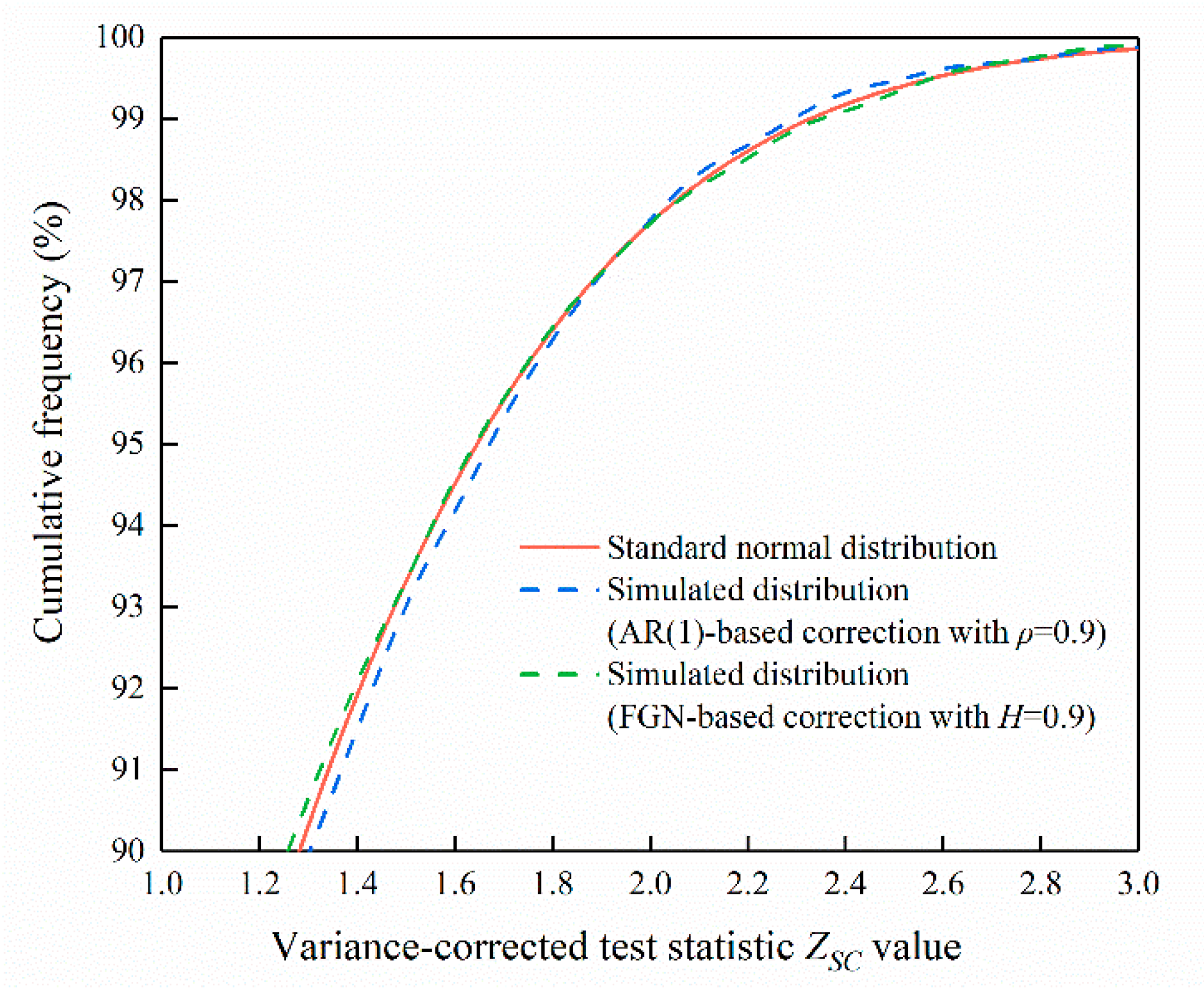
The distribution of the resulting standardized test statistic $Z_{SC}=S/\sqrt{V_C\left(S\right)}$, using the corrected slope variance, was empirically investigated. Figure 4 shows the upper tail of the simulated cumulative distribution of $Z_{SC}$, using 10,000 synthetic AR(1) and FGN data with length $n=100$. Both of the parameters $\rho$ and $H$ were set to 0.9 to represent strong persistent cases. It is clear from Figure 4 that the tail of the standard Normal curve is in good agreement with the tails of $Z_{SC}$ for persistent data. This agreement can be found in cases with lower levels of persistence. Thus, the use of the Normal distribution is still a reasonable approximation to assess the significance of trends in the presence of persistence.

4.2. Practical Procedure of the Method

Using the corrected slope variance described above, an innovative variance-corrected Sen’s trend test can be performed on persistent data. The practical procedure of the method is outlined as follows:

Step 1:

Persistent model specification. The empirical lag-one autocorrelation coefficients of the aggregated time series are plotted versus the time scales. If the lag-one autocorrelations are almost constant or decay slowly for large time scales, the time series is regarded as a representation of an FGN process. Otherwise, the lag-one autocorrelations will drop down to zero after a few time scales; in this case, the time series is classified as an AR(1) process.

Step 2:

Persistent parameter estimation. For the AR(1) data, the empirical lag-one autocorrelation coefficient is estimated from the detrended series, and subsequently bias-corrected as recommended by Hamed [39]: $\rho =\left(n\widehat{\rho }+2\right)/\left(n-4\right)$. For the FGN data, the Hurst coefficient $H$ is estimated via the maximum likelihood method, which has been proven to be robust and to present low bias, as compared to several other methods [40].

Step 3:

Slope variance correction. The corrected slope variance $V_C\left(S\right)$ is calculated using Equation (15) for AR(1) data or Equation (16) for FGN data, according to the results of the persistent model specification.

Step 4:

Trend significance assessment. The variance-corrected test statistic $Z_{SC}$ is compared with the quantiles of the standard Normal distribution at a desired significance level, and the trend significance is quantified.

5. Monte-Carlo Simulation

5.1. Simulation Design

To evaluate the applicability of the proposed method to persistent data, a set of Monte-Carlo simulation experiments were performed. The simulations applied a commonly assumed structure to describe hydrometeorological data, which is a combination of a stationary time series and a linear trend, written by:

$$x_t=A_t+St$$

(17)

where $A_t$ is stationary data exhibiting short-term or long-term persistence, generated by the AR(1) or FGN model, and $S$ is the slope of the linear trend with respect to time $t$.

Type I errors and the power of the test were estimated using the two-sided rejection ratio, given by:

$$\mathrm{Rejection}\mathrm{Ratio}=N_{rej}/N=\left\{\mathrm{Type}\mathrm{I}\mathrm{error},S=0;\mathrm{Power},S\ne 0\right\}$$

(18)

where $N$ is the total number of simulated series (10,000), and $N_{rej}$ is the number of series that the null hypothesis of no trends is rejected by the test. The significance level is assigned at 5% in this study.

The simulations first generated a trendless series with various combinations of series length $n\in \left[30,40,\dots ,200\right]$ and lag-one autocorrelations $\rho \in \left[0,0.1,\dots ,0.9\right]$ to investigate how effectively the procedure of slope variance correction can alleviate Type I error inflation. After correction, the updated slope variance $V_C\left(S\right)$ replaced the original $V_0\left(S\right)$ as the denominator of the variance inflation factor, written as $V\left(S\right)/V_C\left(S\right)$. An effective slope variance correction needs to produce an inflation factor within ±20% from unity, i.e., 0.8–1.2, as suggested by Hamed [39]. According to simulations derived from the standard Normal distribution, which is the approximation of a trend test statistic distribution, the ±20% inflation in variance will result in actual Type I errors of 3.3–6.7% at the 5% level. This margin was determined because perfect correction cannot be achieved unless we can acquire the full knowledge of persistent data, including both the persistent model type and parameter, which is unrealistic in practice.

To highlight the effectiveness of slope variance correction in response to model misspecifications and parameter estimation errors, we discuss simulation results under three special cases. The first case assumes that the real persistent model and its parameter are known before correcting the slope variance. In the second case, the slope variance was corrected using the estimated value of a persistent parameter, where the real persistent model was well-specified. For the last case, attention focuses on the slope variance correction with the wrong choice of persistent model, even though its parameter is correctly identified.

The simulations also generated nonstationary series characterized by an upward linear trend to investigate the power of trend detection under varying levels of data persistence. The dimensionless slope of the linear trend $S/\sigma$ ranges from 0 to 0.05. Power comparisons between Sen’s trend test before and after slope variance correction, as well as the conventional Mann–Kendall test for uncorrelated data, were performed.

5.2. Slope Variance Correction and its Effectiveness on Mitigating Type I Error Inflation

The term “variance correction” means the conversion of the variance of the test statistic under the serial independence assumption into a variance that is appropriate to persistent data. Perfect correction can yield a variance inflation factor of unity, whereby Type I errors will be exactly equal to the significance level. Otherwise, large inflation factors (>1.2) result in unacceptably high Type I errors, namely “under-correction,” while small inflation factors (<0.8) result in too few Type I errors, which is known as “over-correction.”

Table 2. Variance inflation factor of Sen’s slope $V\left(S\right)/V_C\left(S\right)$ after variance correction for AR(1) data. The underlined values denote that the slope variances are “over-corrected” (<0.8) or “under-corrected” (>1.2).

n	$\mathbf{\rho }$
	0	0.1	0.2	0.3	0.4	0.5	0.6	0.7	0.8	0.9
Case I: AR(1)-based correction with a known real value of $\rho$
30	1.00	1.01	1.00	1.00	1.00	1.00	1.00	1.01	1.00	1.00
50	1.00	1.00	1.00	1.00	1.00	1.00	1.00	1.00	1.00	1.00
100	1.00	1.00	1.00	1.00	1.00	1.00	1.00	1.00	1.00	1.00
150	1.00	1.00	1.00	1.00	1.00	1.00	0.99	1.00	1.00	1.00
200	1.00	1.00	1.00	1.00	1.00	1.00	1.00	1.00	1.00	1.00
Case II: AR(1)-based correction with an estimated value of $\rho$
30	0.91	0.91	0.89	0.88	0.89	0.90	0.97	1.22	1.76	2.89
50	0.95	0.94	0.92	0.92	0.90	0.90	0.91	0.95	1.15	2.17
100	0.97	0.96	0.96	0.96	0.95	0.95	0.93	0.91	0.89	1.19
150	0.99	0.98	0.98	0.97	0.97	0.96	0.95	0.94	0.91	0.97
200	0.99	0.99	0.99	0.98	0.98	0.96	0.97	0.96	0.93	0.91
Case III: FGN-based correction with a known real value of Hurst coefficient $H$
30	1.00	0.92	0.88	0.89	0.95	1.07	1.29	1.74	2.61	4.63
50	1.00	0.86	0.78	0.76	0.77	0.84	1.00	1.34	2.16	4.67
100	1.00	0.79	0.66	0.59	0.56	0.59	0.66	0.86	1.41	3.64
150	1.00	0.75	0.60	0.51	0.47	0.47	0.51	0.66	1.05	2.84
200	1.00	0.72	0.55	0.46	0.41	0.40	0.43	0.53	0.84	2.29

and

Table 3. Variance inflation factor of Sen’s slope $V\left(S\right)/V_C\left(S\right)$ after variance correction for FGN data.

n	$\mathbf{\rho }$
	0	0.1	0.2	0.3	0.4	0.5	0.6	0.7	0.8	0.9
Case I: FGN-based correction with a known real value of Hurst coefficient $H$
30	1.00	1.00	1.00	1.00	1.00	1.00	1.00	1.00	1.00	1.00
50	1.00	1.00	1.00	1.00	1.00	1.00	1.00	1.00	1.00	1.00
100	1.00	1.00	1.00	1.00	1.00	1.00	1.00	1.01	1.01	1.00
150	1.00	1.00	1.00	1.00	1.00	1.00	1.00	1.00	1.00	1.00
200	1.00	1.00	1.00	1.00	1.00	1.00	1.00	1.00	1.00	1.00
Case II: FGN-based correction with an estimated value of $H$
30	0.91	1.08	1.24	1.32	1.41	1.49	1.55	1.67	1.75	1.89
50	0.90	1.08	1.16	1.24	1.26	1.32	1.37	1.47	1.56	1.67
100	0.89	1.06	1.11	1.13	1.15	1.15	1.21	1.29	1.37	1.47
150	0.89	1.05	1.09	1.10	1.11	1.13	1.16	1.20	1.26	1.38
200	0.89	1.05	1.07	1.08	1.08	1.10	1.12	1.16	1.21	1.30
Case III: AR(1)-based correction with a known real value of $\rho$
30	1.00	1.09	1.14	1.12	1.06	0.94	0.77	0.58	0.38	0.22
50	1.00	1.17	1.28	1.33	1.29	1.19	1.00	0.74	0.46	0.21
100	1.00	1.27	1.51	1.68	1.77	1.71	1.51	1.16	0.71	0.27
150	1.00	1.34	1.68	1.95	2.14	2.15	1.94	1.53	0.95	0.35
200	1.00	1.39	1.81	2.17	2.44	2.51	2.34	1.87	1.18	0.44

provide the inflation factors after variance correction for AR(1) and FGN data, respectively. The inflation factors are greatly reduced for almost all combinations of $n$ and $\rho$ compared to the original values, as shown in Table 1. The reduction of inflation factors depends on the accuracy of the persistent model specification and parameter estimation. To be specific, nearly perfect correction can be achieved in an ideal case (Case I), where the persistent model and its parameter are exactly known beforehand. In a more practical case (Case II), where the persistent parameters $\rho$ or $H$ are estimated from data, the slope variance is under-corrected for high values of autocorrelation, and the situation occurs with larger autocorrelation as the series length $n$ increases. Case III only produces a narrow band of effective variance correction because of persistent model misspecification. Correcting the slope variance of AR(1) data with an FGN model results in under-correction for high values of autocorrelation and over-correction for a long series. The situation reverses for FGN data, particularly when the slope variance is corrected using an AR(1) model.

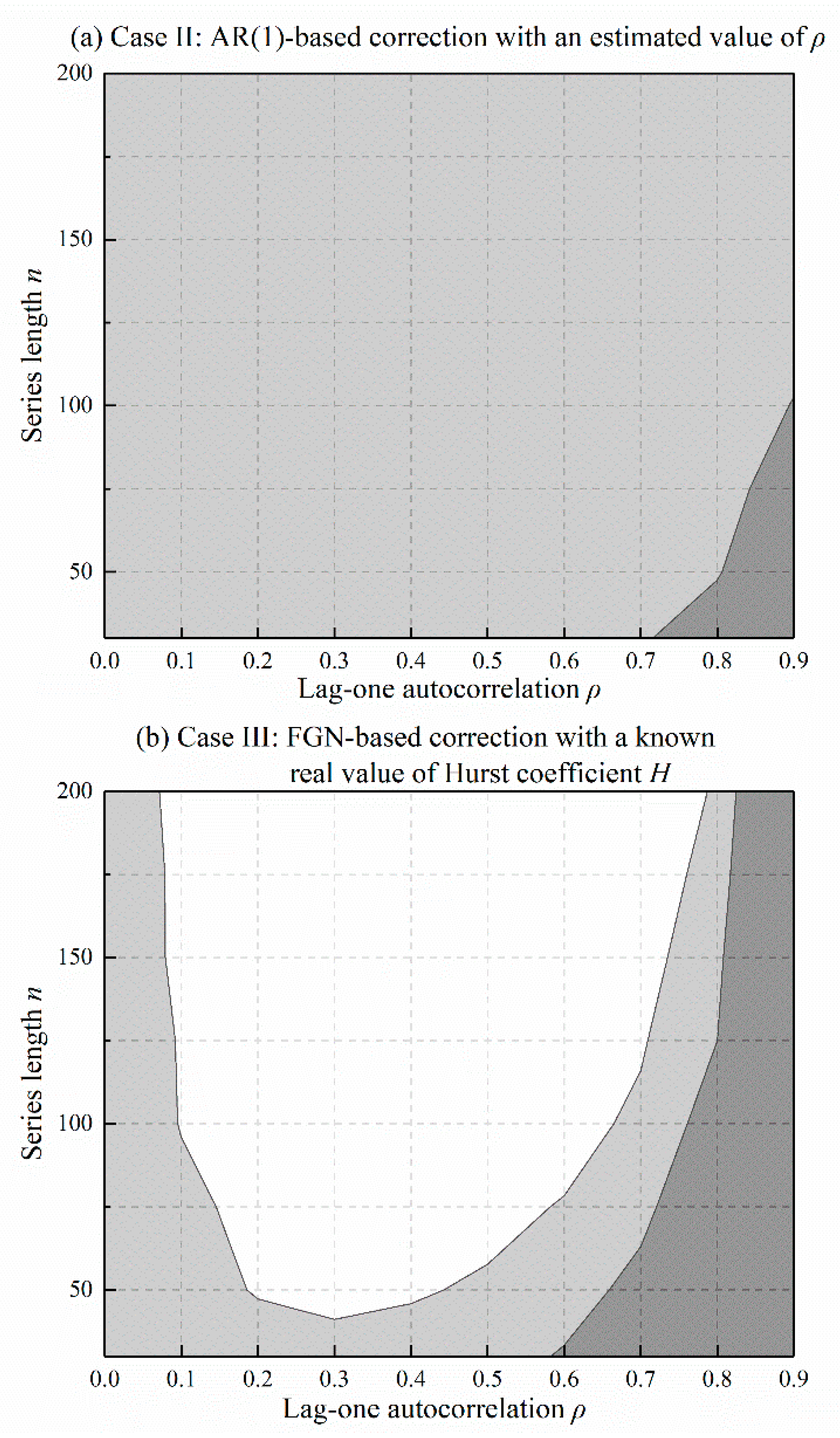
Figure 5 and Figure 6 depict the results of Table 2 and Table 3 using area plots, in which the range of effective slope variance correction is painted in light grey, and the over- and under- correction regions are painted in white and dark grey. In Case II (Figure 4a and Figure 5a), there is a clear trend of increasing acceptable area as the series length increases. In Case III (Figure 4b and Figure 5b), however, longer series do not produce wider acceptable areas. A long series tends to accentuate the discrepancy between the different models, as the data disobeys the hypothetical persistent model. As a result, the corrected test will inflate or deflate Type I errors beyond the acceptable margin of the significance level. To alleviate this weakness, the investigation of the persistent model must be performed initially, as suggested in the practical procedure. Some previous trend studies regarding data pre-whitening have also drawn attention to this serious issue [39,41]. Here, simulation results reinforce the standpoint that model specification is important for trend detection in real persistent hydrometeorological data, especially for long time series.

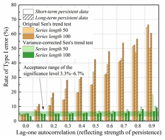
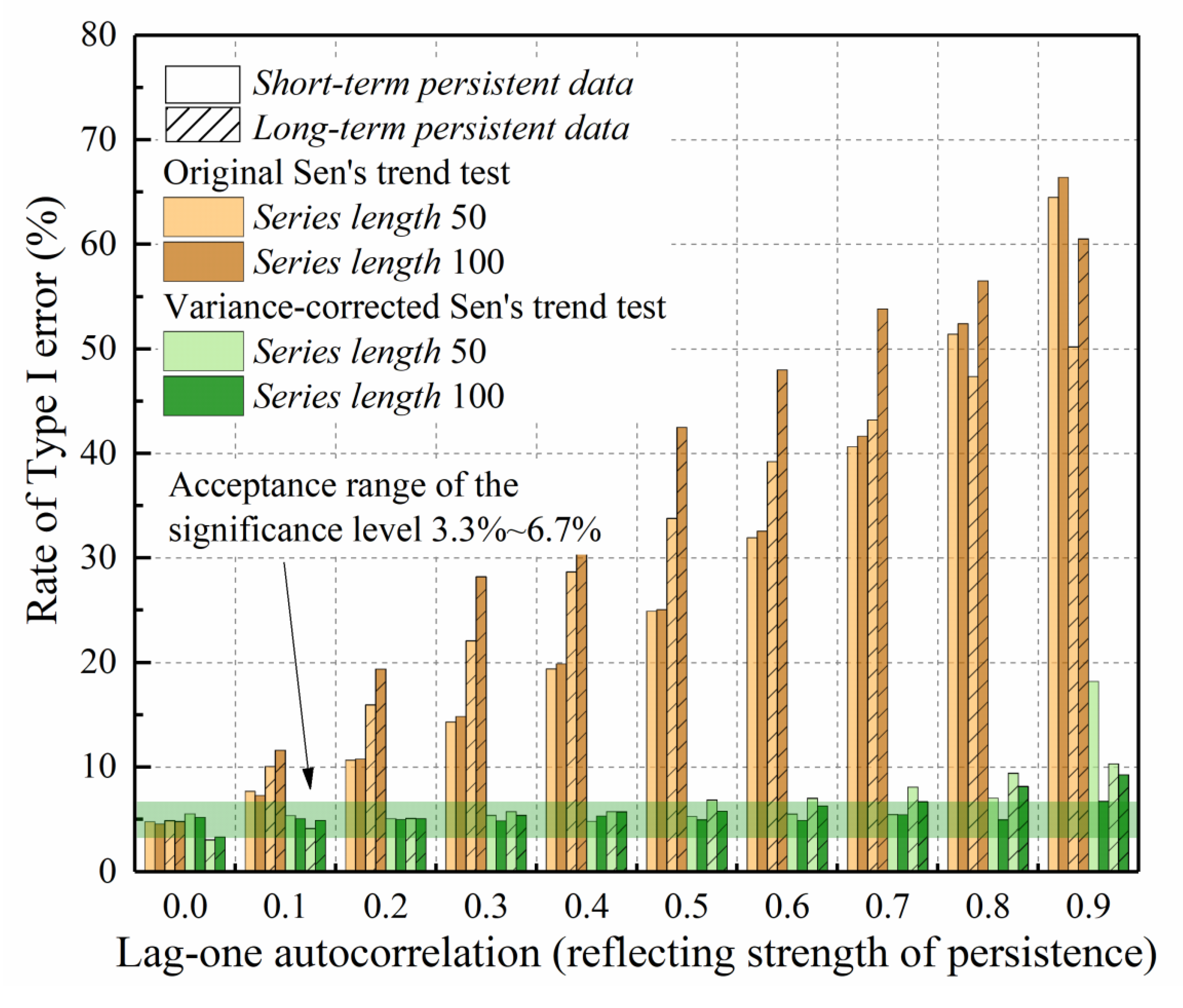
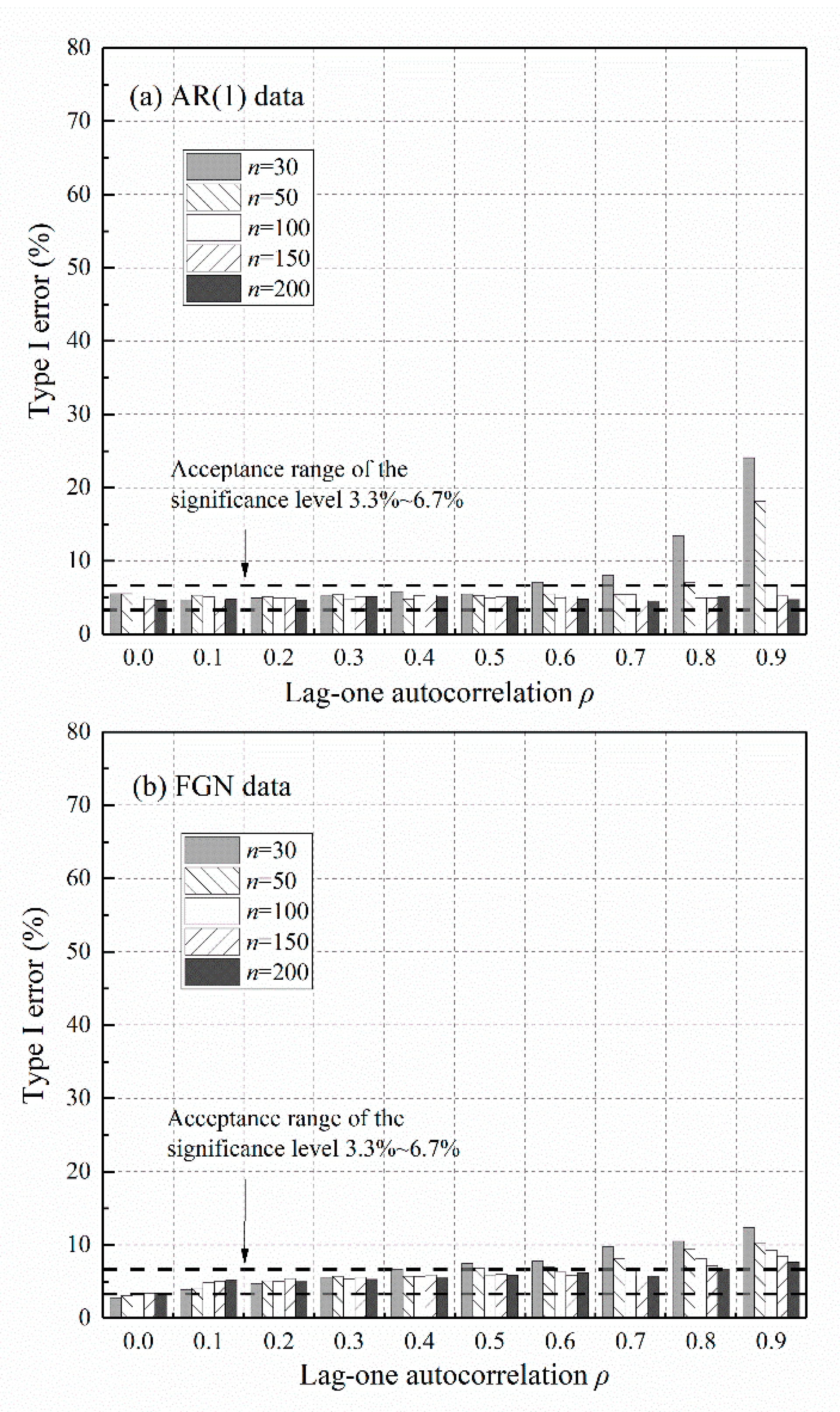
Figure 7 gives Type I errors associated with Sen’s trend test using the correct persistent model. The inflated Type I errors are mostly restored to the acceptance range of the significance level, as opposed to those of the original test given by Figure 3. Considering a series with length $n=100$ for instance, the new test apparently reduces Type I errors of the original test from the range (5–66%) to (5.2–6.7%) for AR(1) data, and from (5–61%) to (3.3–9.3%) for FGN data. Given that persistence in hydrometeorological records such as annual rainfall and runoff are usually moderate, $H\le 0.80$ or equivalently $\rho \le 0.52$, refer to global estimation results of $H$ [37,38]. Thus, the new test requires at least around 50 observations of AR(1) data or 100 observations of FGN data to guarantee acceptable Type I errors. Numerous observations yield better results only if the underlying persistent structure is well specified.

5.3. Power of Trend Detection

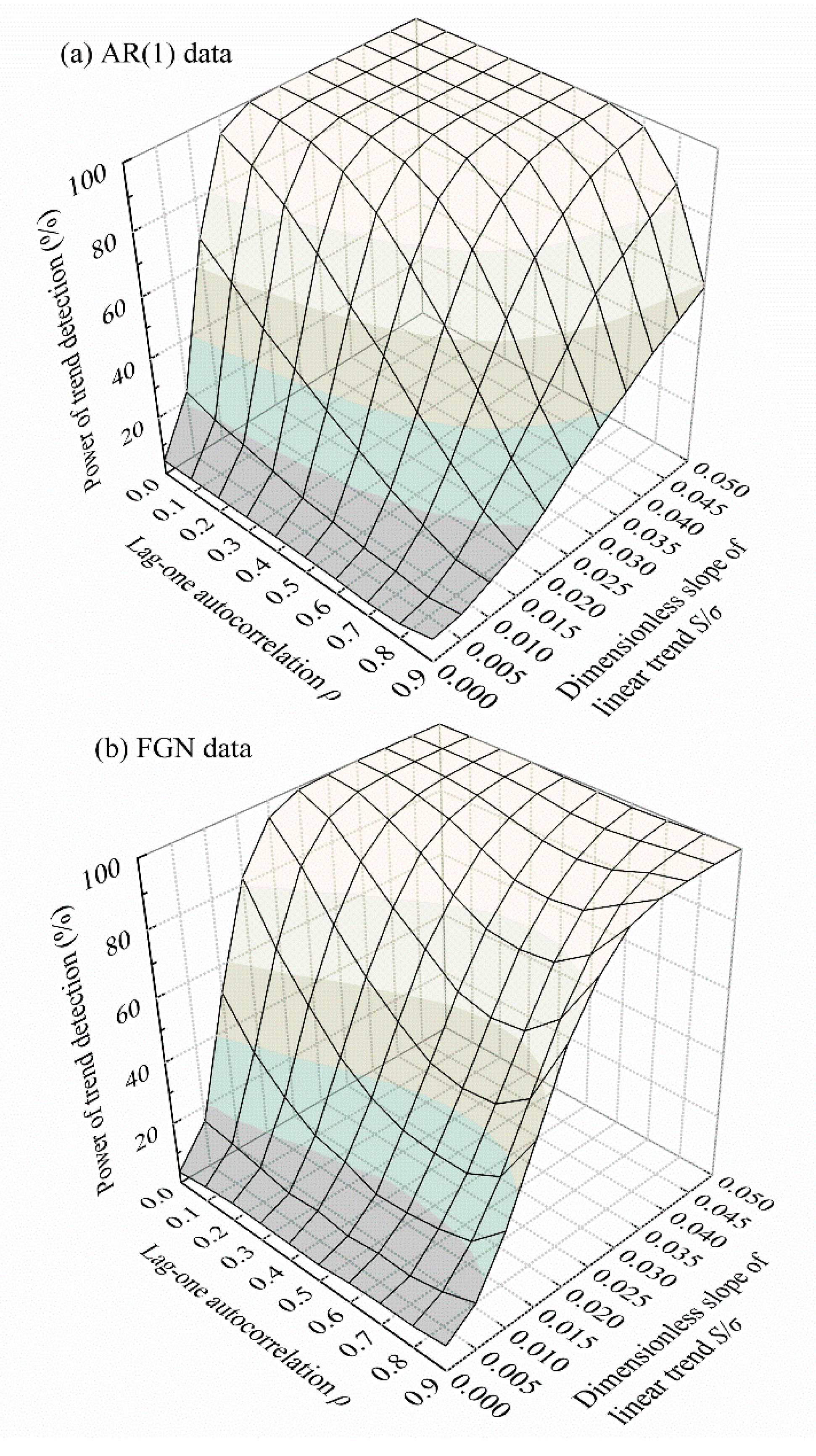
A test is powerful if it can detect weak trends and also maintain an acceptable Type I error. Herein, power curves are presented only in cases where the underlying persistent models are correctly specified, so that the inflated Type I errors can be restored to their normal states. The relationship among power, lag-one autocorrelation (reflecting strength of persistence), and the dimensionless slope of the linear trend for synthetic series with length 100 is depicted in Figure 8. A series length of 100 was chosen simply for illustrative purposes. An analogous pattern of power curves emerges for other series lengths.

The power of the new test is an increasing function of the dimensionless slope of the linear trend, irrespective of data persistence. In general, strong trends in data with weak variation are more likely to be detected than weak trends in highly variable data. In terms of the relationship with data persistence, the power is a monotonic decreasing function of the lag-one autocorrelation for AR(1) data. For FGN data, the power decreases to a minimum at around $\rho =0.6$ and then rises again. Generally, the test is less powerful in detecting a trend in persistent data than in uncorrelated data. This weakness is the so-called power loss. In fact, power loss occurs because of the effect of persistence rather than the procedure of variance correction. Persistence inflates the variance of the trend slope and reduces the value of the test statistic numerically when the null hypothesis is false, thus weakening the ability of the test to detect a real trend from persistent data compared to the case when the same trend exists in uncorrelated data. The power losses depend on the extent of variance inflation. For FGN data, power restoration occurred when $\rho >0.6$, since at that time the inflated variance gradually recovered spontaneously (see Table 1).

Without slope variance correction, the test may prevent power loss at the expense of producing a high Type I error rate, which is far beyond the reported significance level. However, this undermines the fundamental basis for the statistical trend test, which operates by controlling Type I errors within a known significance level, signifying users’ confidence toward detected trends.

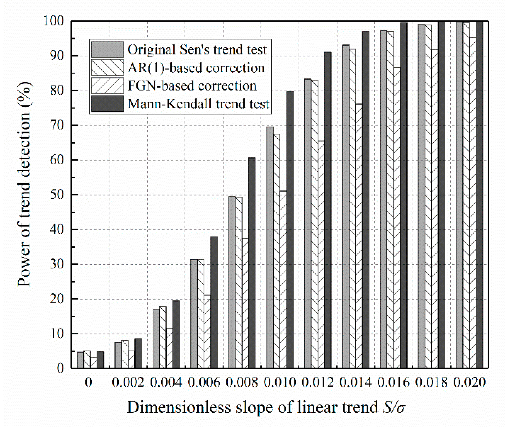
Sen’s trend test with the help of slope variance correction is built for persistent data. When the data are independent of time, will this manipulation reduce the power? The answer is given in Figure 9. The power of the test based on AR(1) correction is comparable to that of the original. However, the test based on FGN correction becomes less powerful, because of the sampling errors introduced by the Hurst coefficient estimation. This finding reasserts the importance of careful choice of a persistent model before performing variance correction. Revisiting the first step of the practical procedure, independent data can be classified as a special case of an AR(1) process. Thus, the adoption of AR(1)-based correction would not cause an apparent loss of power.

Figure 9 also reveals that Sen’s trend test is less powerful than the Mann–Kendall test for uncorrelated data with weak trends. However, the power of Sen’s trend test achieves that of the Mann–Kendall test as the slope of the trend increases. This argues against the statement made by earlier comparison studies that Sen’s trend test can identify many significant trends ignored by the Mann–Kendall test [19,42]. The discrepancy mainly arises from the incorrect slope variance, Equation (3), given by Sen [11]. In Section 2.2, it was demonstrated that this slope variance is substantially biased even for independent data. The expression should be replaced by a bias-corrected expression, Equation (4), so that the Type I error rate can return to its normal state. However, the power will be slightly lower than the Mann–Kendall test.

6. Application to Real-World Data

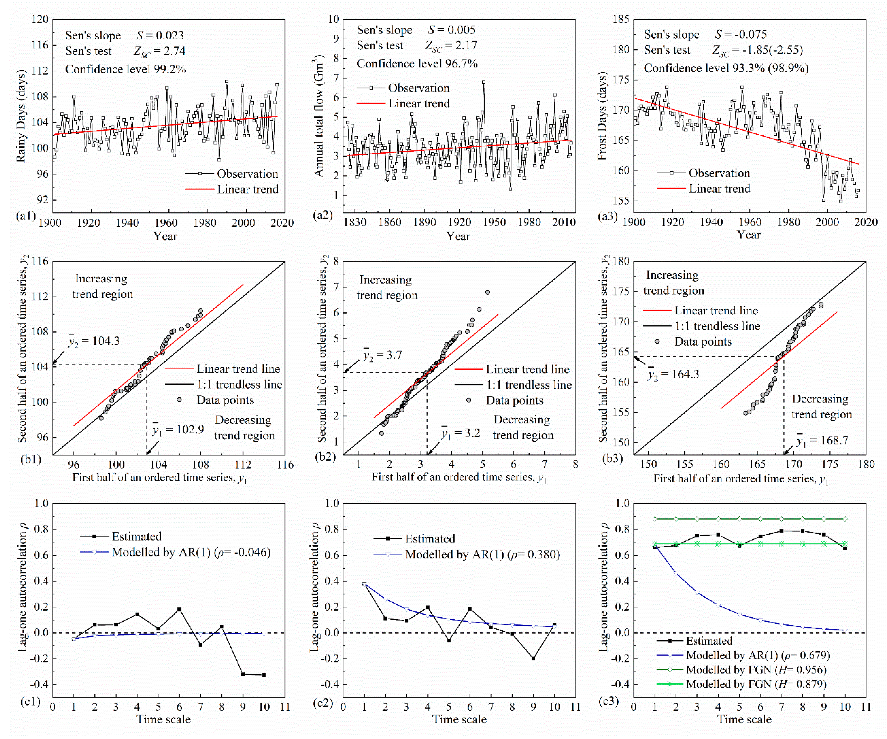
Hydrometeorological variables carries different persistence characteristics, for example independence, short-term, and long-term persistence. To demonstrate the applicability of the new method on series with different degree of persistence, three real-world records were selected for illustration, including rainy days, frost days, and streamflow. The annual series of rainy days, and frost days of China were obtained from the CRU CY 4.01 dataset (1901–2016), produced by the Climate Research Unit at the University of East Anglia [43]. The annual total flow (1824–2016) from Main River at Wuerzburg in Germany were kindly provided by the Global Runoff Data Centre in Koblenz, Germany (http://grdc.bafg.de).

The time series plot and its corresponding 1:1 trend plot are presented in Figure 10a,b. In the time series plots, increasing trends are recognizable in rainy days and annual total flow, and decreasing trends in frost days for the entire record. The 1:1 trend plots provide detailed information about sub-trends. Regarding the rainy days, the trend slopes at higher values are generally stronger than that for the lower value cases. The annual total flow series shares a similar behavior. The increasing trend is dominated by high values. In addition, the low cluster is almost trend-free, whereas an apparent reduction occurs at the extremely low values. In the series of frost days, downward trends are prevalent throughout high, medium, and low clusters and the trends are dominant in the low cluster.

The persistence features of the three series were further examined by plotting the empirical lag-one autocorrelation of the aggregated series versus time scale, as depicted in Figure 10c. The trajectories of the theoretical autocorrelations of AR(1) and FGN models are also depicted in the same figure. The maximum scale of aggregation was set to ten, assuring that each aggregated series contains at least ten values. The rainy days exhibit low autocorrelations, which fluctuate around zero initially and become negative for large scales. The series is generally independent of time, and therefore we can regard the series as a representation of AR(1) data. The autocorrelations of annual total flow fluctuate around the value modelled by AR(1). Annual total flow is thus very likely to be AR(1) data. The long-term persistence of the frost days is clear in this example. Autocorrelation appears to be constant. Thus, the FGN model is a better approximation of the underlying process.

Table 4. Results of Sen’s trend test before and after slope variance correction.

Variables	Statistical Features		Data Persistence		Slope Variance		Test Statistic 1
	Mean $\mathbf{\mu }$	$\mathbf{Slope}\mathit{S}/\mathbf{\sigma }$	Model	Parameter	$\mathbf{Original}{\mathit{V}}_0\left(\mathit{S}\right)$	$\mathbf{Corrected}{\mathit{V}}_{\mathit{C}}\left(\mathit{S}\right)$	$\mathbf{Original}{\mathit{Z}}_{\mathit{S}}$	$\mathbf{Corrected}{\mathit{Z}}_{\mathit{S}\mathit{C}}$
Rainy days	103 days	0.008	AR(1)	$\rho =-0.046$	7.9 × 10−5	7.2 × 10−5	2.62 ++	2.74 ++
Annual total flow	3.44 Gm3	0.005	AR(1)	$\rho =0.380$	2.1 × 10−6	4.5 × 10−6	3.22 ++	2.17 +
Frost days	166 days	−0.017	FGN	$H=0.956$ (0.879)b	0.2 × 10−3	0.2 × 10−2 (0.9 × 10−3)	−5.18 ++	−1.85 (−2.55 +)

¹ Significant trends at the $5\%$ ($\left|Z\right|>1.96$) level are indicated by “⁺”, at the $1\%$ ($\left|Z\right|>2.576$) level by “⁺⁺”; ² Values in parentheses are the Hurst coefficients estimated from the detrended series and the corresponding slope variance and trend test statistic.

gives the trend detection results when applying the original and variance-corrected Sen’s trend test. The second and third columns show the basic statistical features of the series. The specified persistent model and its parameter are provided in the next two columns. In the frost days, the high value of the Hurst coefficient is in doubt because the existence of a real trend may result in overestimation. As such, the Hurst coefficient was also estimated from the detrended series (in parentheses) for comparison. The last four columns indicate the original and corrected slope variances and their corresponding trend test statistics. The new method only slightly alters the trend test statistic of rainy days, which is nearly independent of time. As for the persistent series, the new method effectively reduces the inflated statistic values. The confidence level (one minus significance level) of increasing annual total flow and decreasing frost days drops from 99% to 95%, when the effect of persistence is taken into account. The new method even rejects significant trend of frost days, when we corrected the slope variance using the higher estimate of the Hurst coefficient.

This result indicates a possibility that the statistical evidences of trends within many hydrometeorological processes are overestimated because of the ignorance of the intrinsic characteristic of persistence. Admitting persistence in the new Sen’s trend test helps to avoid exaggerating trend significance and overuse of deterministic trends. In practical applications, properly accounting for deterministic t rends and persistent behavior are inherently linked with understanding and modelling hydrometeorological processes. On the one hand, the persistent process implies that there is nontrivial dependence between the present state and the previous states, and the handling of dependence in prediction model can be made through reasoning future state conditional on the known past information. Dependence improves one-step-ahead predictability in comparison to purely random process. On the other hand, the persistent process exhibits much wide range of natural variability at large time scales. Many statistical characteristics become time-related. For example, local means may vary in time and fluctuate irregularly around the global mean. This enhanced fluctuation reduce predictability of the process over long time horizon. The detected trend would initiate an investigation on the causative effects through deductive reasoning and data validation. The trend if at all valid can enrich our knowledge of the changes in external forces and in internal conditions of the hydrometeorological systems.

In the current application, increasing trend of annual rainy days was detected in China, which is a manifestation of precipitation regime changes. Decreasing frost days is an evidence of global warming over mainland China. But the statistical significance of trend markedly reduced when the long-term persistence is considered. Similar reductions in the significance of rising temperature are also evidenced by other studies [44,45]. We argue that the future evolution of temperature-like processes would be much more uncertain than we perceive. Annual total flow from Main River in Germany exhibits both the short-term persistence and the increasing trend. This feature reveals that the Main River was generally enriched, yet had a propensity of enduring consecutive years of natural excursions from the mean. This information has evident implication for the designing, operation, and management of hydro projects.

7. Conclusions

This study adapts the recently proposed Sen’s trend test to persistent data via a variance correction approach. Two expressions for the variance of the trend test statistic were newly derived under the assumption of persistence. One variance is tailored to short-term persistent data, characterized by the AR(1) model. The other expression is designed for long-term persistent data and is represented by the FGN model. The computation of these new variances is convenient, as they only require one additional parameter, i.e., the lag-one autocorrelation coefficient or Hurst coefficient. We also fixed the original variance for independent data, thereby correcting its negative bias.

An innovative variance-corrected Sen’s trend test was developed with the aid of newly derived variances. Simulation results verified the effectiveness of the new test on alleviating the side effect of persistence. By correcting the variance with the most approximate persistent model of the data, the rate of committing Type I errors remains within an acceptable range of the nominal significance level. The power of trend detection monotonically increases for higher trend slopes. The power losses depend on how much the persistence inflates the variance of the trend test statistic. The more seriously inflated the variance, the less powerful the test. A stepwise procedure was recommended for performing the new test on real hydrometeorological observations. Case studies explained in detail how to differentiate independent, short-term persistent, and long-term persistent data, so as to invoke the corresponding variance prudently.

The actual advantage of the Sen’s trend detection method is to deduce the overall trend and hidden sub-trends in various categories simultaneously on a furnished 1:1 trend plot. The flexible categorization of observations provides detailed information about the trend characteristics for each cluster. However, in the context of trend significance analysis, Sen’s trend test does not perform better than the conventional Mann–Kendall test. The purported novelty of Sen’s trend test, i.e., it is free of any restrictive assumptions, is not supported by the current study. This finding renders some published trends based on the original Sen’s trend test problematic and may therefore need to be reassessed. The proposed new Sen’s trend test attaches its test statistic to the distinctive persistent feature of hydrometeorological data. Sen’s trend plot with the help of variance-corrected Sen’s trend test yields more reliable statistical evidence of the changes occurring and sheds light on the future evolution of hydrological and climatic processes.

References

- IPCC. Summary for Policymakers. In Global Warming of 1.5 °C; An IPCC special report on the impacts of global warming of 1.5 °C above pre-industrial levels and related global greenhouse gas emission pathways, in the context of strengthening the global response to the threat of climate change, sustainable development, and efforts to eradicate poverty; 2018; in press. [Google Scholar]
- Jimenez Cisneros, B.E.; Oki, T.; Arnell, N.W.; Benito, G.; Cogley, J.G.; Doll, P.; Jiang, T.; Mwakalila, S.S. Freshwater Resources. In Climate Change 2014: Impacts, Adaptation, and Vulnerability. Part A: Global and Sectoral Aspects; Contribution of working group II to the Fifth Assessment Report of the Intergovernmental Panel on Climate Change; Cambridge University Press: Cambridge, UK; New York, NY, USA, 2014. [Google Scholar]
- Durocher, M.; Requena, A.I.; Burn, D.H.; Pellerin, J. Analysis of trends in annual streamflow to the Arctic Ocean. Hydrol. Process. 2019, 33, 1143–1151. [Google Scholar] [CrossRef]
- Arora, R.; Tockner, K.; Venohr, M. Changing river temperatures in northern Germany: Trends and drivers of change. Hydrol. Process. 2016, 30, 3084–3096. [Google Scholar] [CrossRef]
- Gao, T.; Wang, H. Trends in precipitation extremes over the Yellow River basin in north China: Changing properties and causes. Hydrol. Process. 2017, 31, 2412–2428. [Google Scholar] [CrossRef]
- Hodgkins, G.A.; Dudley, R.W.; Archfield, S.A.; Renard, B. Effects of climate, regulation, and urbanization on historical flood trends in the United States. J. Hydrol. 2019, 573, 697–709. [Google Scholar] [CrossRef]
- Yeste, P.; Dorador, J.; Martin-Rosales, W.; Molero, E.; Esteban-Parra, M.J.; Rueda, F.J. Climate-driven trends in the streamflow records of a reference hydrologic network in southern Spain. J. Hydrol. 2018, 566, 55–72. [Google Scholar] [CrossRef]
- Garbrecht, J.; Fernandez, G.P. Visualization of trends and fluctuations in climatic records. Water Resour. Bull. 1994, 30, 297–306. [Google Scholar] [CrossRef]
- Basarin, B.; Lukic, T.; Pavic, D.; Wilby, R.L. Trends and multi-annual variability of water temperatures in the river Danube, Serbia. Hydrol. Process. 2016, 30, 3315–3329. [Google Scholar] [CrossRef] [Green Version]
- Sen, Z. Innovative trend analysis methodology. J. Hydrol. Eng. 2012, 17, 1042–1046. [Google Scholar] [CrossRef]
- Sen, Z. Innovative trend significance test and applications. Theor. Appl. Climatol. 2017, 127, 939–947. [Google Scholar] [CrossRef]
- Sen, Z. Trend identification simulation and application. J. Hydrol. Eng. 2014, 19, 635–642. [Google Scholar] [CrossRef]
- Wu, H.; Qian, H. Innovative trend analysis of annual and seasonal rainfall and extreme values in Shaanxi, China, since the 1950s. Int. J. Climatol. 2017, 37, 2582–2592. [Google Scholar] [CrossRef]
- Caloiero, T.; Coscarelli, R.; Ferrari, E. Application of the innovative trend analysis method for the trend analysis of rainfall anomalies in southern Italy. Water Resour. Manag. 2018, 32, 4971–4983. [Google Scholar] [CrossRef]
- Dabanli, I.; Sen, Z.; Yelegen, M.O.; Sisman, E.; Selek, B.; Guclu, Y.S. Trend assessment by the innovative-Sen method. Water Resour. Manag. 2016, 30, 5193–5203. [Google Scholar] [CrossRef]
- Belihu, M.; Abate, B.; Tekleab, S.; Bewket, W. Hydro-meteorological trends in the Gidabo catchment of the Rift Valley Lakes basin of Ethiopia. Phys. Chem. Earth 2018, 104, 84–101. [Google Scholar] [CrossRef]
- Cui, L.F.; Wang, L.C.; Lai, Z.P.; Tian, Q.; Liu, W.; Li, J. Innovative trend analysis of annual and seasonal air temperature and rainfall in the Yangtze River basin, China during 1960–2015. J. Atmos. Sol. Terr. Phys. 2017, 164, 48–59. [Google Scholar] [CrossRef]
- Kisi, O. An innovative method for trend analysis of monthly pan evaporations. J. Hydrol. 2015, 527, 1123–1129. [Google Scholar] [CrossRef]
- Zhou, Z.G.; Wang, L.C.; Lin, A.W.; Zhang, M.; Niu, Z.G. Innovative trend analysis of solar radiation in China during 1962–2015. Renew. Energy 2018, 119, 675–689. [Google Scholar] [CrossRef]
- Kisi, O.; Ay, M. Comparison of Mann–Kendall and innovative trend method for water quality parameters of the Kizilirmak River, Turkey. J. Hydrol. 2014, 513, 362–375. [Google Scholar] [CrossRef]
- Deng, S.L.; Chen, T.; Yang, N.; Qu, L.; Li, M.C.; Chen, D. Spatial and temporal distribution of rainfall and drought characteristics across the Pearl River basin. Sci. Total Environ. 2018, 619, 28–41. [Google Scholar] [CrossRef]
- Tosunoglu, F.; Kisi, O. Trend analysis of maximum hydrologic drought variables using Mann–Kendall and Sen’s innovative trend method. River Res. Appl. 2017, 33, 597–610. [Google Scholar] [CrossRef]
- O’Connell, P.E.; Koutsoyiannis, D.; Lins, H.F.; Markonis, Y.; Montanari, A.; Cohn, T. The scientific legacy of Harold Edwin Hurst (1880–1978). Hydrol. Sci. J. 2016, 61, 1571–1590. [Google Scholar] [CrossRef]
- Sen, Z.K. Hydrological trend analysis with innovative and over-whitening procedures. Hydrol. Sci. J. 2017, 62, 294–305. [Google Scholar] [CrossRef]
- Burger, G. On trend detection. Hydrol. Process. 2017, 31, 4039–4042. [Google Scholar] [CrossRef]
- Hamed, K.H. Trend detection in hydrologic data: The Mann–Kendall trend test under the scaling hypothesis. J. Hydrol. 2008, 349, 350–363. [Google Scholar] [CrossRef]
- Wang, W.; Chen, Y.; Becker, S.; Liu, B. Linear trend detection in serially dependent hydrometeorological data based on a variance correction Spearman Rho method. Water 2015, 7, 7045–7065. [Google Scholar] [CrossRef]
- Koutsoyiannis, D. The Hurst phenomenon and Fractional Gaussian Noise made easy. Hydrol. Sci. J. 2002, 47, 573–595. [Google Scholar] [CrossRef]
- Hurst, H.E. Long-term storage capacity of reservoirs. Trans. Am. Soc. Civ. Eng. 1951, 116, 770–808. [Google Scholar]
- Mandelbrot, B.B.; Wallis, J.R. Some long-run properties of geophysical records. Water Resour. Res. 1969, 5, 321–340. [Google Scholar] [CrossRef] [Green Version]
- Koutsoyiannis, D. Climate change, the Hurst phenomenon, and hydrological statistics. Hydrol. Sci. J. 2003, 48, 3–24. [Google Scholar] [CrossRef]
- Koutsoyiannis, D. Nonstationarity versus scaling in hydrology. J. Hydrol. 2006, 324, 239–254. [Google Scholar] [CrossRef] [Green Version]
- Koutsoyiannis, D. Hydrology and change. Hydrol. Sci. J. 2013, 58, 1177–1197. [Google Scholar] [CrossRef]
- Matalas, N.C.; Sankarasubramanian, A. Effect of persistence on trend detection via regression. Water Resour. Res. 2003, 39, 1342. [Google Scholar] [CrossRef]
- Dimitriadis, P.; Koutsoyiannis, D. Stochastic synthesis approximating any process dependence and distribution. Stoch. Environ. Res. Risk Assess. 2018, 32, 1493–1515. [Google Scholar] [CrossRef]
- Tsoukalas, I.; Makropoulos, C.; Koutsoyiannis, D. Simulation of stochastic processes exhibiting any-range dependence and arbitrary marginal distributions. Water Resour. Res. 2018, 54, 9484–9513. [Google Scholar] [CrossRef]
- Iliopoulou, T.; Papalexiou, S.M.; Markonis, Y.; Koutsoyiannis, D. Revisiting long-range dependence in annual precipitation. J. Hydrol. 2018, 556, 891–900. [Google Scholar] [CrossRef]
- Markonis, Y.; Moustakis, Y.; Nasika, C.; Sychova, P.; Dimitriadis, P.; Hanel, M.; Maca, P.; Papalexiou, M. Global estimation of long-term persistence in annual river runoff. Adv. Water Resour. 2018, 113, 1–12. [Google Scholar] [CrossRef]
- Hamed, K.H. Enhancing the effectiveness of prewhitening in trend analysis of hydrologic data. J. Hydrol. 2009, 368, 143–155. [Google Scholar] [CrossRef]
- Tyralis, H.; Koutsoyiannis, D. Simultaneous estimation of the parameters of the Hurst-Kolmogorov stochastic process. Stoch. Environ. Res. Risk Assess. 2011, 25, 21–33. [Google Scholar] [CrossRef]
- Serinaldi, F.; Kilsby, C. The importance of prewhitening in change point analysis under persistence. Stoch. Environ. Res. Risk Assess. 2016, 30, 763–777. [Google Scholar] [CrossRef]
- Li, J.; Wu, W.; Ye, X.; Jiang, H.; Gan, R.; Wu, H.; He, J.; Jiang, Y. Innovative trend analysis of main agriculture natural hazards in China during 1989–2014. Nat. Hazards 2018, 95, 677–720. [Google Scholar] [CrossRef]
- Harris, I.; Jones, P.D.; Osborn, T.J.; Lister, D.H. Updated high-resolution grids of monthly climatic observations—The CRU TS3.10 dataset. Int. J. Climatol. 2014, 34, 623–642. [Google Scholar] [CrossRef]
- Cohn, T.A.; Lins, H.F. Nature’s style: Naturally trendy. Geophys. Res. Lett. 2005, 32, L23402. [Google Scholar] [CrossRef]
- Ludescher, J.; Bunde, A.; Franzke, C.L.E.; Schellnhuber, H.J. Long-term persistence enhances uncertainty about anthropogenic warming of Antarctica. Clim. Dyn. 2016, 46, 263–271. [Google Scholar] [CrossRef]
Figure 1.
Illustration of linear trend identification with Sen’s method: (a) Time series and trend; (b) Sen’s trend plot.
Figure 2.
Comparison between the simulated distribution of the test statistic for stationary independent data of length and the corresponding Normal approximation: (a) original test statistic (Sen, 2017a); (b) bias-corrected test statistic.
Figure 3.
The effect of data persistence on Type I errors of the original Sen’s trend test: (a) AR(1) data; (b) Fractional Gaussian Noise (FGN) data.
Figure 4.
The upper tail of the simulated cumulative distribution of the test statistic after variance correction for AR(1) and FGN data as compared to the standard Normal distribution.
Figure 5.
Effectiveness of variance correction for AR(1) data. Light gray shading indicates acceptable region. White and dark grey shading indicate over-and under-correction, respectively.
Figure 6.
Effectiveness of variance correction for FGN data.
Figure 7.
Type I errors of the variance-corrected Sen’s trend test using a well-specified persistent model: (a) AR(1) data; (b) FGN data. The persistent parameters and are estimated from the data.
Figure 8.
Power of the variance-corrected Sen’s trend test with various combinations of data persistence and a dimensionless slope of linear trend (series length: ) using a well-specified persistent model: (a) AR(1) data; (b) FGN data. The persistent parameters and are estimated from the data.
Figure 9.
Power of the innovative variance-corrected Sen’s trend test compared to that of the original test and the Mann–Kendall test, for the case of uncorrelated data (series length: ).
Figure 10.
Time series of annual rainy days and frost days of China (a1,a3), and annual total flow from Main River at Wuerzburg in Germany (a2). Trend test results given in (a1–a3) are obtained from variance-corrected Sen’s trend test. Sen’s trend plots for the data sets in a1–3 (b1–b3). Lag-one autocorrelations of the aggregated series versus time scales as for a1–3 (c1–c3).