Design Equation for Stirring Fluid by a Stream Pump in a Circulating Tank


Faculty of Civil and Environmental Engineering, Gdansk University of Technology,80-233 Gdańsk, Poland
*
Author to whom correspondence should be addressed.
Water 2019, 11(10), 2114; https://doi.org/10.3390/w11102114
Submission received: 13 August 2019
/
Revised: 30 September 2019
/
Accepted: 9 October 2019
/
Published: 12 October 2019
(This article belongs to the Section Hydraulics and Hydrodynamics)
Abstract
:A circulating tank is a very useful theoretical scheme for many fluid-flow objects in several branches of engineering. The motion of the fluid in such objects can be induced in different ways. A stream pump provides an especially interesting possibility; however, the quantitative description of such devices shows some shortcomings. Such a device is analogous to a jet pump, thus has similar advantages (simplicity of construction, lack of movable elements, insensibility to pollutants) and disadvantages (low efficiency). On the one hand, from the technical viewpoint, one can make use of technical instructions presented in handbooks and offered by producers, and on the other hand by performing calculations using CFD tools. In this situation, it is self-evident that some intermediary method of design, i.e., formally simple, but physically convincing, would be welcome both by theoreticians and by engineers. Such a method is proposed in this paper and takes the form of an algebraic formula, combining the discharge of the stream pump and the discharge of the circulation induced by this stream. This expression, based on the balance between the power of the stream and the power of dissipation, has been experimentally verified with a positive result.
1. Introduction
The stirring (or agitation) of fluid-containing systems consists of so many aspects and variants that its complete description would probably be impossible. The more so, because human invention still brings new solutions and ideas. A returnable flow must be recognized as a necessary condition of the considered process. It can appear in various geometrical scales—from very small scale, locally (e.g., in air bubble aeration systems), to large scale, defined by chamber dimensions (circulation) [1].
A very important and interesting category of stirring objects can be found in biologically active structures. An activated sludge reactor can serve as a classic example of this category, especially the modern kind of these types of chambers, which give the possibility of wastewater denitrification and dephosphatation [2].
Breeding pools in seal sanctuaries or similar marine facilities can act as the next example. The water which fills these basins contains many harmful components (remains of food, animal excrement, hair of periodically molting seals…), which must be kept in suspension to be eliminated by a stream of flowing water, refreshing the basin contents.
These stirring needs can be fulfilled using different technical solutions. Here, the application of stream pumps seems especially attractive [3,4]. The discharge and orientation (direction of the stream) can be flexibly controlled, creating the required velocity field in the basin.
The problem is that the qualitative theory of the operation of stream pumps is relatively well described for their classic form, when they work as jet pumps, which operate on the basis of the Venturi effect (drop of pressure in a nozzle throat), well recognized and described in the bibliography [5,6]. In the situation considered here, when we only want to induce the circulation of a liquid in a chamber, the literature of the problem is very poor. Hence, the subject of this text is the formulation of a technically acceptable design equation for this application of stream pumps.
The main premise of the paper is the formal simplicity of the final result, supported by its practically positive physical accuracy. This is a very important statement, as in each case, anybody interested in such a device design, will reach for CFD methods [7,8]. But in everyday technical (and even scientific) practice, it is very useful to have at one’s disposal some simplified methods which can be applied, at least for making preliminary calculations, but also to support the process of numerical simulation.
2. Theoretical Considerations
2.1. General Concept of the Proposed Mathematical Model
Let us stress that we are looking for a mathematically simple and, simultaneously, physically sensible expression. Therefore, the simple and credible law of nature is needed. The balance of the power introduced into the chamber by the stream pump (Pin) and the power dissipated by the circulating liquid (Pdis) provides a very interesting possibility. In a steady state, usually considered as a conclusive situation, both these powers are equal:
This equality has been effectively applied in many particular forms—for aerated grit chambers [9], for air lift pumps [10], for vortex grit separators [11], or vortex flow regulators and storm overflows [12]. The theoretical rudiments of this concept for turbulent flow conditions are described in the paper [13]. In the theory of mixing, the power of dissipation is willingly expressed by the velocity gradient [14], more or less precisely [15], and then combined with the other physical variables (especially with the mixing time), using empirical relations. These relations are presented in scientific and technical handbooks (e.g., [16,17]) or in the form of technical instructions, suggested by the producers of the devices under consideration.
In this paper, a particular case of stirring flow has been considered, namely the circular flow of a liquid (especially water or wastewater) in an open channel, forming a closed loop. When the pump works, the liquid filling the channel is sucked in by the inlet (discharge QS) and then—injected back to the channel through the outlet. Liquid introduced in this way forms a submerged stream the kinetic energy of which is passed to the ambient liquid, inducing the circulation (discharge QR) [18].
2.2. Assumptions and Simplifications
It is evident that the chance of formulating a prospective relation exists only for geometrically simple and regularsystems. For complex objects, built-up in three dimensions, which are described by partial differential equations, one cannot hope for anappropriate algebraic notation. This means that some simplifying assumptions are necessary.
Therefore, in the paper only one-dimensional fluid-flow structures will be considered, when the mean velocity can be used as a kinematic parameter: νS for the nozzle outlet:
and νR – tangent to the wall component of the liquid circulation:
If we want to obtain a technically suitable relation between QS and QR, this restriction is obvious. It can be easily accepted for the circulation in a chamber, but creates more doubt when a submerged jet is considered. It is well known [18] that the diameter of the jet increases, which means that there exists a transversal component of motion, which can also generate a crosswise flow in a channel. Alas, an algebraic description of the energy dissipation intensity would not be possible. Fortunately, the classical 1D model of a submerged stream works well in technical problems, thus Equation (2) has been accepted in this paper. Nonetheless, one should be aware that such an underestimation of the energy loss will probably cause an overestimation of the calculated discharge QR.
The next simplification raises the assumption that the only factor which creates the circulation is the jet energy (discharge QS), whereas in the neighborhood of the pump inlet a second stream will be formed (effect of pump suction), which can also influence the circulation. However, according to the theory of submerged jets, this rear stream is much wider, even 2–3 times, than the frontal one. One can easily observe this effect by use of a vacuum cleaner and the smoke from incense burning without a flame. As it is shown below (Equation (4)), the energy of a stream decreases with the fourth power of its diameter. Assuming that the rear stream is two times wider than the first one, its energy would be 16 times lower. This means that this factor can be neglected in the energy balance.
Analyzing the energy balance, one should remember that the total power of dissipation Pdis results from the liquid circulation losses Pdiss and the direct energy dissipation inside the submerged stream Pdisj. The first factor regards the whole channel, whereas the second is a local one (as it is known from the jets theory [18], such structure very quickly loses its dynamic distinction) and must be described by the differential equations of the theory of turbulence. These equations are formally complex, so description of Pdisj by the mathematically simple algebraic expressions (what is a basic postulate of this paper) would not be possible. In this situation the jest dissipation power Pdisj was neglected. Permissibility of this simplification was evaluated empirically. In the other words it was assumed, that if the theoretical relation QR(QS) is accepted (at least from the technical point of view), the omission of Pdisj will be reasonable.
All these assumptions and simplifications lower the accuracy of the proposed method and define its limitations. However, the expected equation must have some good technical qualities so even a coarse evaluation can be of avail.
2.3. Determination of the Induced Power
The power delivered by the stream pump into the liquid which fills the chamber can be expressed by the well-known technical expression:
where: QS, QR—discharges of the stream pump and the channel, respectively, vS—mean velocity in the pump outlet, dS—diameter of the pipe outlet.
2.4. Determination of the Dissipation Power
To obtain a desired (i.e., mathematically simple) form of the design equation, the power of dissipation must be expressed by technically justified values (discharge of the channel QR, mean velocity in the channel vR, channel geometry: Length L, width B, depth H, radii of the bend curvatures, if necessary), making use of classical hydraulic methods. Such an attitude is very often applied, especially in practically oriented investigations of fluid-flow systems, like pipes (e.g., [19]) or open channels (e.g., [20]).
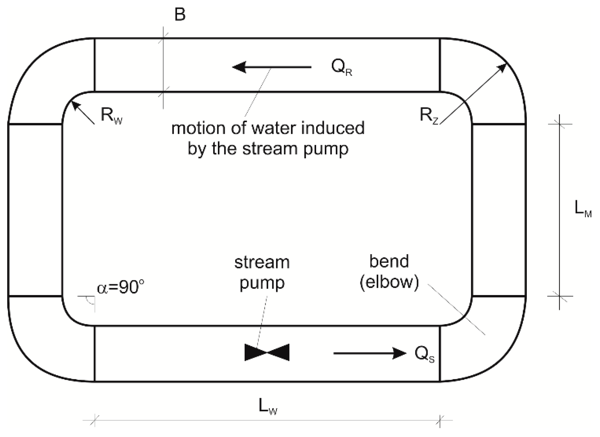
The structures under consideration (i.e., circulating tanks) usually have regular shapes, thus, remaining at quite a high level of generality, we can accept the calculation scheme as shown in Figure 1.
In order to calculate (with technical precision) the intensity of the energy dissipation during the circulation (according to the assumed 1D model of the flow), one has to fit the coefficients of hydraulic loss for each particular hydraulic element of the channel. In each situation, one has to take into account the individual features of the system, so further considerations will have an exemplary, but still quite general, character.
As a source of information about these coefficients, a classic handbook [21] was used. The calculation scheme shown in Figure 1 consists of four bends (elbows 90°) and four straight pipe segments. Moreover, one should take into account here the presence of the body and supporting holder of the stream pump, which, being the propulsion of circulation, also prove some hydraulic resistance.
The coefficient of hydraulic loss caused by one bend can be calculated from the following formula (reference velocity for this coefficient: vR, Equation (3) [21]:
where: R0—radius of the bend, RH—hydraulic radius:
F0—channel cross-section, WP—channel wetted perimeter, λ—Nikuradse hydraulic loss coefficient, α—angle of the bend (in this case α = 90°). The bend radius is equal to (Figure 1):
The energy loss coefficient for the four straight segments is given by the well-known Darcy–Weisbach formula (reference velocity: Equation (3)):
As regards the coefficient of hydraulic loss caused by the stream pump, one has at one’s disposal some further possibilities, depending on the individual shape of the device. A review of the already mentioned handbook [19] leads to the conclusion that this object can be treated as a single square beam, and the main parameter of its resistance is the proportion between the total (i.e., including the support and conduits) frontal surface of the pump Fsand the channel cross-section F0. If so, the minor loss coefficient for the stream pump equals [21]; reference velocity: Equation (3):
Hence, the summary head of the mechanical energy loss in the channel is related to the mean velocity of the liquid, and equals:
The mean velocity of the circulation was expressed by Equation (3). The effective loss coefficient is equal to:
This means that the total power of dissipation in the chamber amounts to:
2.5. Proposed Design Equation
According to Equation (1), we can compare Equation (4) and Equation (12), which yields the final relation between the discharge in the circulation chamber QR and the discharge of the stream pump QS, inducing the motion in this chamber:
3. Experimental Verification
3.1. Laboratory Stand
In order to obtain an experimental verification of the proposed formula (Equation (13)), some laboratory investigations of the discussed object have been carried out.
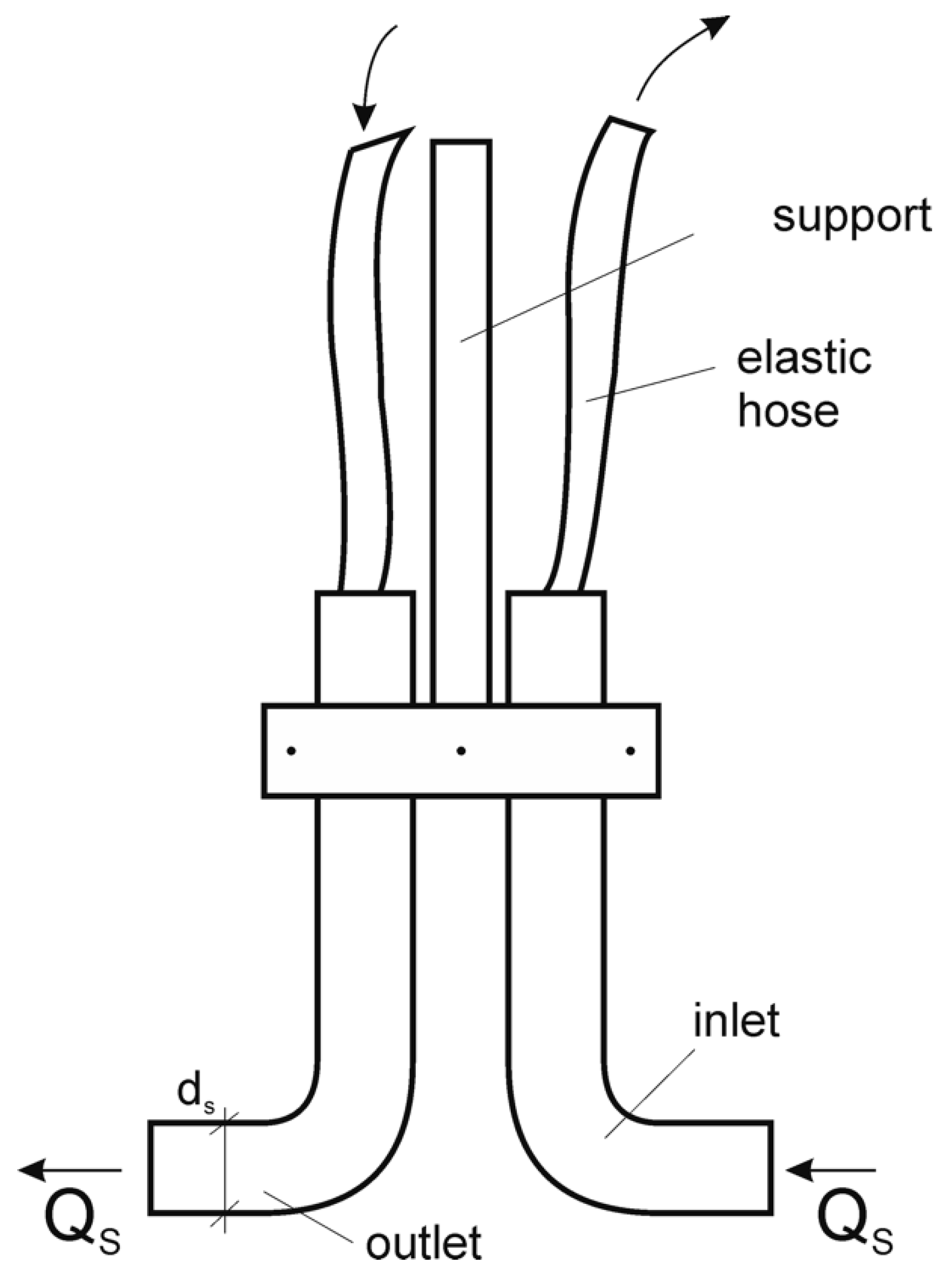
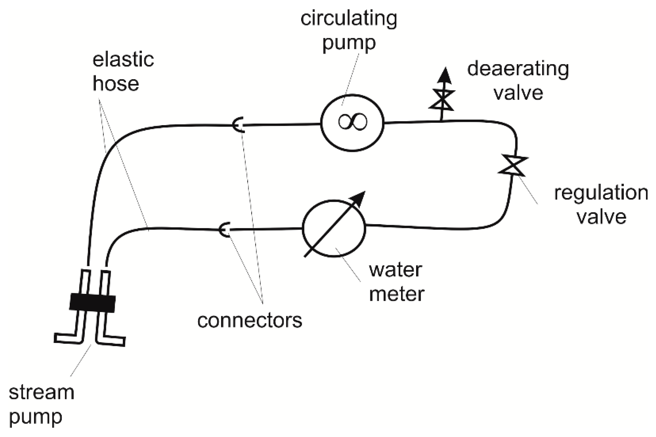
The stream pumps under consideration were made of the standard stainless-steel fittings usually used in pneumatic installations, according to the scheme shown in Figure 2. The inlet and outlet elbows were joined together with a typical connection clip and equipped with a simple support, joining the pump with the chamber wall. The inlet and the outlet were connected (through the elastic hose) with the drive unit, containing a circulating pump (25 POr 60C, Grundfoss), a vane-wheel water meter (Metron JS 1,5) serving the pump discharge QS determination and two valves—for regulation and deaeration (Figure 3). In each investigated case, the time tV of flow of V = 10 liters of water was recorded (from 100 to 200 seconds, depending on the actual pump setting). The time tV was measured manually, making use of a laboratory electronical stop watch. The volume V was read from the water meter counter. The accuracy of this measurement was equal to 5% (as the precision of the used device, determined according to European standards MID, equals 2% for the highest flows and 5% for the lowest; in the presented case the minimal acceptable water discharge was equal 0.03 m3/h, maximal acceptable discharge—3–12 m3/h and minimal measured discharge was equal to 0.23 m3/h).The actual value QS was measured two times for each pump setting, after the flow stabilization—at the outset and the end of each run and averaged. The discharge was calculated as follows:
It is worth noting that in practical applications, both the inlet and outlet could be combined together with the other elements. However, such a device would obviously have bigger dimensions, and in addition—the conductors delivering the electric current should be thoroughly protected (especially important in breeding basins for sea mammals).
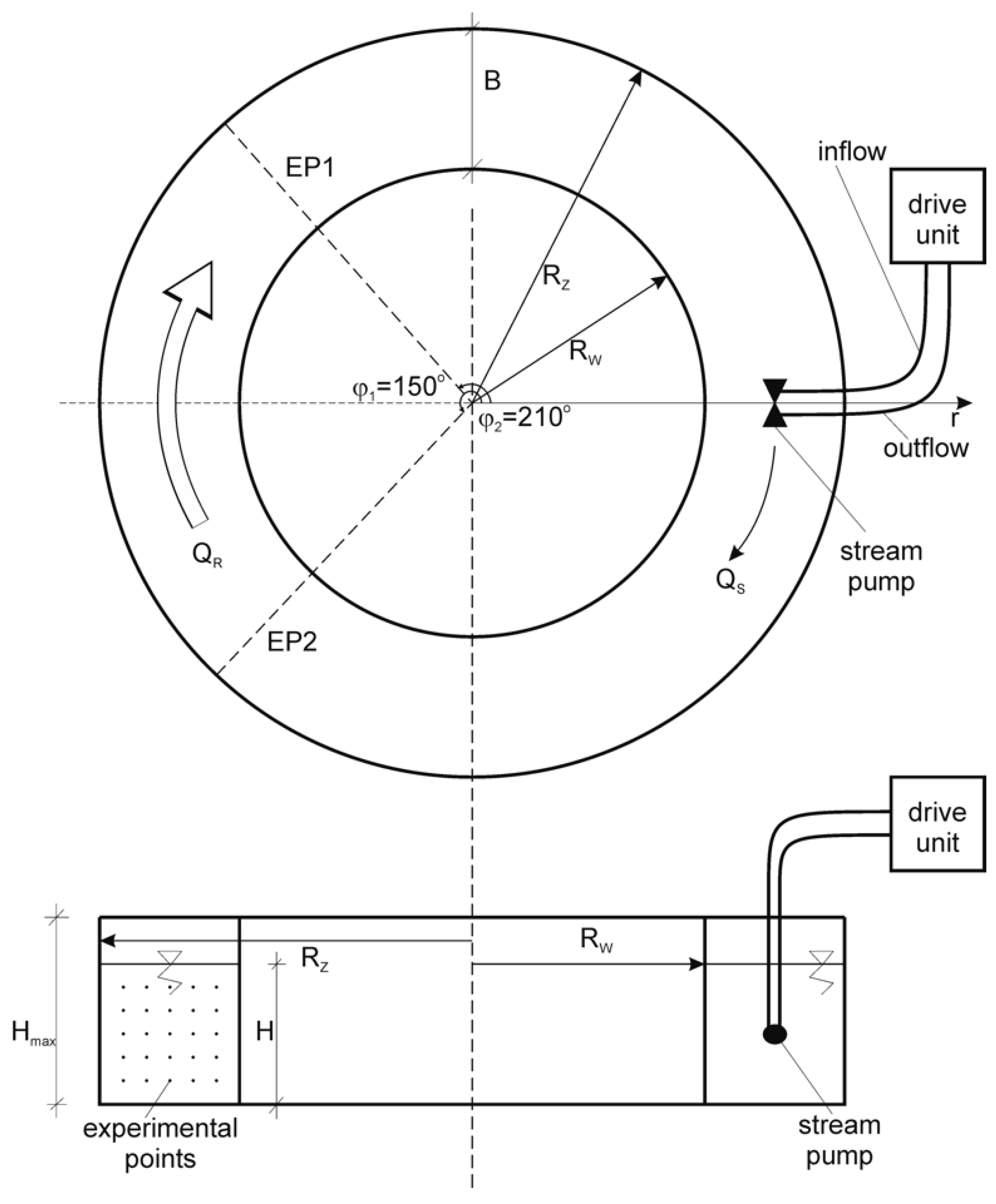
When it comes to the chamber, where the circulation must be induced, one has to consider a large number of different solutions. Taking into account that we are going to formulate a formally simple (although justified from the physical point of view) design formula, combining the discharge of the pump QS, the discharge of the circulation QR and the device geometry, a search was carried out for a very regular form of the channel—i.e., a circular chamber, which was made of a stainless steel sheet. Its main dimensions equal RZ = 0.4 m, RW = 0.2 m, Hmax = 0.3 m (Figure 4).
During the assembling of the stand, special attention was paid to the proper orientation of the nozzle, as the jet should be tangent to the wall. For this purpose, a small dose (5 ml) of a dye (water solution of Rhodamine WT) was introduced into the stream pump. The colored jet was observed and the direction of the nozzle was corrected.
As it was already mentioned, the measurements were performed when the flow was stabilized in time. When the pump was switched on, the laboratory stand was observed and the local velocity was measured in the central point of the section EP1, making use of a velocity meter. The time of the flow stabilization was determined experimentally. It was stated that it lasted 1 hour from setting the pump.
The local tangential velocity of the circulating liquid uφ was measured in two sections (for φ1 = 150° and φ2 = 210°) in 16 regularly distributed points in each section (Figure 4), making use of a 16 MHz MicroADV (acoustic Doppler velocimeter)produced by Sontek.Basic characteristics of the ADV sensor: Measurement frequency 0.1–50 Hz, range of velocity measured 0.001 m/s–2.5 m/s, minimum measuring error 0.0025m/s, resolution 0.0001 m/s, measurement cell 0.09 cm3, measurement point distance 0.05 m [22]. Measurements were made with 1 Hz frequency samplingfor 1 minutes in every point. Minimumvalue of correlation ratio above 80% and signal-to-noise ratio (SNR) above 18 dBresult high accuracy. In the above-mentioned conditionsthe manufacturer declares measuring error Δ = 1% of measured value (but not less than 0.0025 m/s) [22]. Using one instrument ADV, the local velocity was measured n each point (with relative measurement uncertainty ±Δ), one after another, for the sector EP1 in the first place and afterwards—EP2.The chamber discharge was calculated by the numerical integration of the measured velocity distribution, according to the classical relation:
3.2. Measurement Results
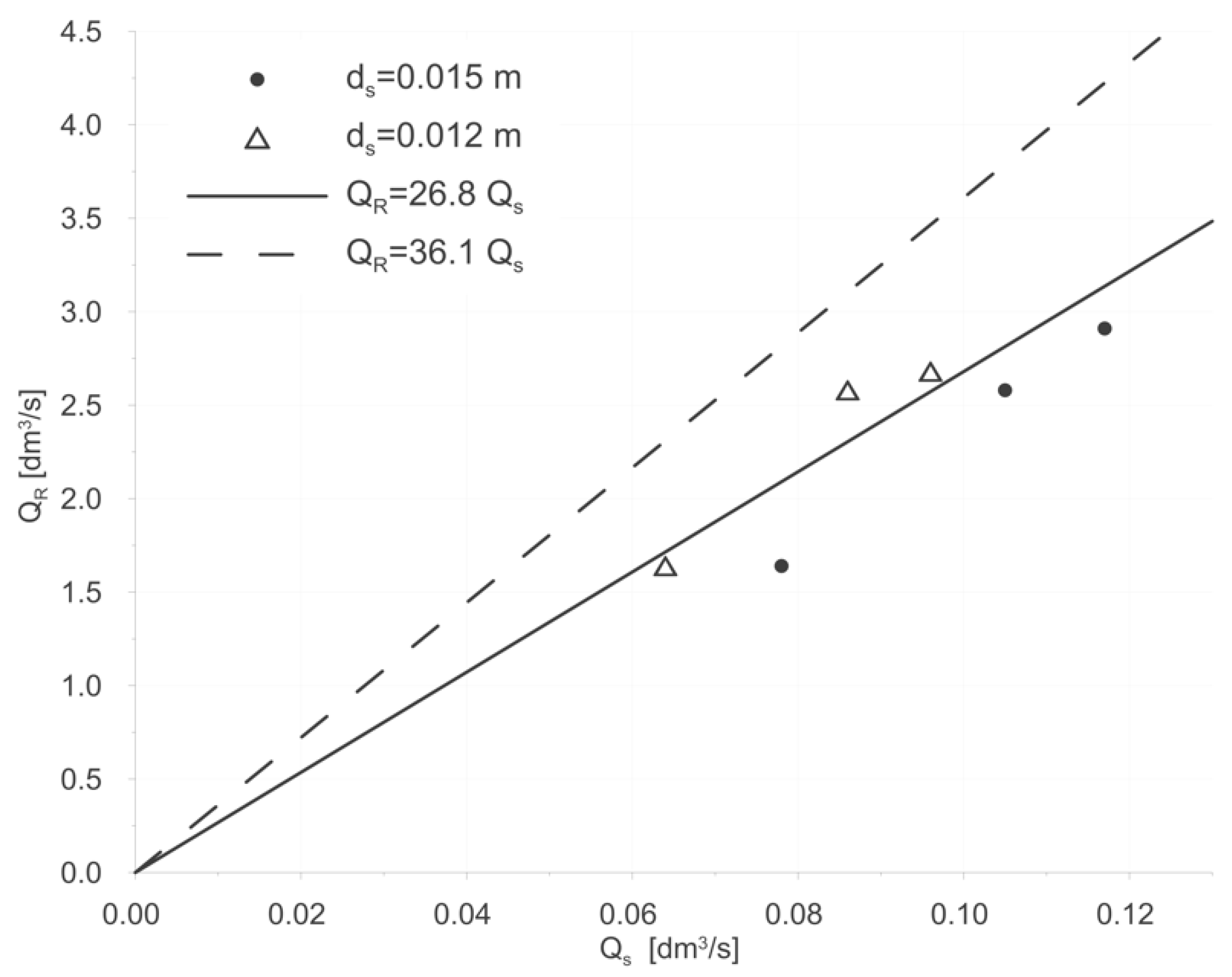
The measurements were performed in the manner described above, for two versions of the stream pump—dSA = 0.015 m and dSB = 0.012 m, for some different depths of the channel. An example of these results (for H = 0.215 m) is presented below:
and shown in Figure 4 as two sets of experimental points, for both pumps.
dSA = 0.015 m: QS = 7.8 × 10⁻⁵ m3/s — QR = 1.85 × 10⁻³ m3/s;
QS = 1.05 × 10⁻⁴ m3/s — QR = 2.58 × 10⁻³ m3/s;
QS = 1.17 × 10⁻⁴ m3/s — QR = 2.91 × 10⁻³ m3/s;
dSB = 0.012m: QS = 6.4 × 10⁻⁵ m3/s — QR = 1.64 × 10⁻³ m3/s;
QS = 8.6 × 10⁻⁵ m3/s — QR = 2.30 × 10⁻³ m3/s;
QS = 9.6 × 10⁻⁵ m3/s — QR = 2.68 × 10⁻³ m3/s,
QS = 1.05 × 10⁻⁴ m3/s — QR = 2.58 × 10⁻³ m3/s;
QS = 1.17 × 10⁻⁴ m3/s — QR = 2.91 × 10⁻³ m3/s;
dSB = 0.012m: QS = 6.4 × 10⁻⁵ m3/s — QR = 1.64 × 10⁻³ m3/s;
QS = 8.6 × 10⁻⁵ m3/s — QR = 2.30 × 10⁻³ m3/s;
QS = 9.6 × 10⁻⁵ m3/s — QR = 2.68 × 10⁻³ m3/s,
3.3. Verification of the Proposed Equation
For the presented case, i.e., the cylindrical chamber shown in Figure 4, we have B = RZ − RW = 0.2 m and H = 0.215 m. According to the procedure described above, we can calculate the geometrical parameters of the object: F0 = 0.043 m2, WP = 0.63 m, RH = 0.068 m (Equation (6)), R0 = 0.3 m (Equation (7)), LW = LM = 0, α = 90°.
Hence, the coefficient of the minor loss for a single bend—ζb = 0.286 (Equation (5)—it was assumed, that λ = 0.05), coefficient ζl = 0 (Equation (8)) and the coefficient of loss caused by the stream pump—ζs = 0.967 (Equation (10), assuming that the pump covers about 15% of the channel cross-section, i.e., Fz/F0 = 0.15). One should remember about the energy loss caused by the ADV velocity meter. It was assumed that the body of this device is analogical to the pump body, and twice the value of ζs, so finally, the effective coefficient of energy loss was equal to:
and now we can formulate the relation between QR and QS. According to Equation (11) we have:
Diagrams of these functions are shown in Figure 5, together with two sets of experimental points.
According to the simple theoretical model proposed in this paper, the relation QR(QS) is a linear function. This result has been confirmed by the experiments, both qualitatively and (what is much more important)—quantitatively. The difference between the calculations and measurements is close to 9.3% (for dS = 0.015 m) and 25% (for dS = 0.012 m), with a mean value of 17%. However, the model proposed above does not pretend to be a precise theory. From the definition, this suggestion must be a method for the technical evaluation of the discharge in a circulating tank (Figure 6), induced by a stream pump. From this point of view, one should appraise this concept positively.
4. Conclusions
A circulating tank is an important hydraulic scheme which appears in many different technical objects. A fluid drive, and especially—stream pumps, can be considered as advantageous sources of circulation energy. In the bibliography, there lack simple relations combining the discharge of circulation with the discharge of the stream pump inducing this motion. For this reason, it would be very purposeful to develop a mathematically simple (although physically justified) method, describing the considered question.
Such a method has been proposed in this paper. It is based on the balance of the energy introduced into the tank, and the energy dissipated during the circular motion, and takes the attractive form of an algebraic relation (Equation (13)). This is worth saying that the formal simplicity and algebraic character determines the novelty of the presented method of calculations and hence— the proposed relation (Equation (13)). This relation has been positively verified empirically. One has to admit that at about 17%, the accuracy of this tool is not very high, but as an evaluation of the real course of this phenomenon, it is fully acceptable. The proposed formula gives an overestimated evaluation of the relation QR(QS), which is a consequence of the introduced simplifications. This approach can be applied in each technical situation, where one has to do with a circulating flow. Some possible kinds of problems were mentioned in the introduction. Especially interesting object looks to be the Carrousel system of the activated sludge reactors, serving for biological waste water treatment. This solution is very attractive and becomes more and more popular of late decades. The waste water circulation in such reactors can be induced by the stream pumps and the proposed formula can be used for the rough (but very quick) and preliminary calculation of the pump setting and the object regulation.
The research presented in this paper gives opportunity of an interesting and useful continuation. In the first order a fluid flow circulative object (when the reverse motion described above is superimposed with an outer stream, forced by the inlet channel energy), which represents an important hydraulic scheme of some waste water treatment reactors (Carrousel type), will be investigated. The velocity field in such chamber will be calculated by means of CFD methods, verified empirically and then the detention time distribution will be investigated, especially—measured during the tracer investigations, using a fluorometric method (Rhodamine WT, fluorometers Cyclops 7 and Trilogy by Turner Design, USA). On the base of these results some practical conclusions, regarding the design and operation of such devices, will be drawn.
Author Contributions
Conceptualization: J.S.; methodology: J.S. and P.Z.; software: P.Z. and P.W.; validation: P.Z.; formal analysis: P.Z.; investigation: P.Z. and P.W.; resources: P.W.; data curation: P.Z. and P.W.; Writing—Original draft preparation: J.S.; Writing—Review and editing: J.S. and P.W.; visualization: P.W.; supervision: J.S.; project administration: P.Z.; funding acquisition: J.S.
Funding
This research was funded by the EU project “Innovative resources and effective methods of safety improvement and durability of buildings and transport infrastructure in sustainable development”. The APC was funded by the European Fund of Regional Development.
Conflicts of Interest
The authors declare no conflict of interest.
References
- Shah, M. Course Material Process Engineering: Agitation Mixing. Available online: http://www.dduanchor.org/site/wp-content/uploads/2014/11/Process-Engineering-Agitation-Mixing.pdf (accessed on 13 August 2019).
- Demirel, E.; Aral, M.M. Unified Analysis of Multi-Chamber Contact Tanks and Mixing Efficiency Based on Vorticity Field. Part I: Hydrodynamic Analysis. Water 2016, 8, 495. [Google Scholar] [CrossRef]
- Maruyama, T.; Ban, Y.; Mizushina, T. Jet mixing of fluids in tanks. J. Chem. Eng. Jpn. 1982, 15, 342–348. [Google Scholar] [CrossRef]
- Matej, K.; Pawliczka, I.; Sawicki, J.M.; Wielgat, P.; Zima, P. Whirling System of Water Exchange in Breeding Pools. Arch. Hydro-Eng. Environ. Mech. 2016, 63, 253–263. [Google Scholar] [CrossRef] [Green Version]
- Higgins, H.W. Water Jet Air Pump Theory and Performance; Pennsylvania State University: State College, PA, USA, 1964. [Google Scholar]
- Wilman, J.T. Jet Pumps; European Atomic Energy Community—EURATOM Reactor Centrum Nederland—RCN: Brussels, Belgium, 1966. [Google Scholar]
- Zima, P.; Makinia, J.; Swinarski, M.; Czerwionka, K. Effects of different hydraulic models on predicting longitudinal profiles of reactive pollutants in activated sludge reactors. Water Sci. Technol. J. Int. Assoc. Water Pollut. Res. 2008, 58, 555–561. [Google Scholar] [CrossRef] [PubMed]
- Zima, P.; Makinia, J.; Swinarski, M.; Czerwionka, K. Combining computational fluid dynamics with a biokinetic model for predicting ammonia and phosphate behavior in aeration tanks. Water Environ. Res. Res. Publ. Water Environ. Fed. 2009, 81, 2353–2362. [Google Scholar] [CrossRef] [PubMed]
- Sawicki, J.M. Aerated Grit Chambers Hydraulic Design Equation. J. Environ. Eng. 2004, 130, 1050–1058. [Google Scholar] [CrossRef] [Green Version]
- Sawicki, J.M.; Pawłowska, A. Energy balance for air lift pumps. Arch. Hydro-Eng. Environ. Mech. 1999, 46, 63–72. [Google Scholar]
- Gronowska-Szneler, M.A.; Sawicki, J.M. Simple design criteria and efficiency of hydrodynamic vortex separators. Water Sci. Technol. J. Int. Assoc. Water Pollut. Res. 2014, 70, 457–463. [Google Scholar] [CrossRef] [PubMed]
- Mielczarek, S.; Sawicki, J.M. Dimensioning of vortex storm overflows. Water Sci. Technol. J. Int. Assoc. Water Pollut. Res. 2018, 78, 259–265. [Google Scholar] [CrossRef] [PubMed]
- Artichowicz, W.; Sawicki, J.M. Determination of Mechanical Energy Loss in Steady Flow by Means of Dissipation Power. Arch. Hydro-Eng. Environ. Mech. 2017, 64, 73–85. [Google Scholar] [CrossRef] [Green Version]
- Slattery, J.C. Advanced Transport Phenomena; Cambridge University Press: Cambridge, UK, 1999; ISBN 978-1-316-58390-6. [Google Scholar]
- Luo, C. Distribution of Velocities and Velocity Gradients in Mixing and Flocculation Vessels: Comparison between LDV Data and CFD Predictions. Ph. D. Thesis, New Jersey Institute of Technology, Newark, NJ, USA, 1997. [Google Scholar]
- Kasat, G.R.; Pandit, A.B. Mixing Time Studies in Multiple Impeller Agitated Reactors. Can. J. Chem. Eng. 2004, 82, 892–903. [Google Scholar] [CrossRef]
- Dickley, S.D. Minimize Blending Time. Available online: https://www.chemicalprocessing.com/articles/2009/120/ (accessed on 12 August 2019).
- Abramovich, G.N.; Schindel, L. The Theory of Turbulent Jets; MIT-Press: Cambridge, UK, 2003; ISBN 978-0-262-01008-5. [Google Scholar]
- Qiao, Q.S.; Choi, K.W.; Chan, S.N.; Lee Joseph, H.W. Internal Hydraulics of a Chlorine Jet Diffuser. J. Hydraul. Eng. 2017, 143, 06017022. [Google Scholar] [CrossRef]
- Das, B.S.; Khatua, K.K. Flow Resistance in a Compound Channel with Diverging and Converging Floodplains. J. Hydraul. Eng. 2018, 144, 04018051. [Google Scholar] [CrossRef]
- Idelchik, I.E.; Ginevskiĭ, A.S. Handbook of Hydraulic Resistance, 4th ed.; rev. and augmented.; Begell House: Redding, CT, USA, 2007; ISBN 978-1-56700-251-5. [Google Scholar]
- SonTek/YSI, Inc. ADVField/Hydra Acoustic Doppler Velocimeter (Field) Technical Documentation; SonTec: San Diego, CA, USA, 2001. [Google Scholar]
Figure 1.
Generalized shape of a circulating tank.

Figure 2.
Sketch of a stream pump.

Figure 3.
Sketch of a drive unit.

Figure 4.
Measuring stand.

Figure 5.
Sketch of the investigated circulating tank: plan view and axial cross-section.

Figure 6.
Comparison of calculated and measured results.

© 2019 by the authors. Licensee MDPI, Basel, Switzerland. This article is an open access article distributed under the terms and conditions of the Creative Commons Attribution (CC BY) license (http://creativecommons.org/licenses/by/4.0/).
Share and Cite
MDPI and ACS Style
Sawicki, J.; Wielgat, P.; Zima, P. Design Equation for Stirring Fluid by a Stream Pump in a Circulating Tank. Water 2019, 11, 2114. https://doi.org/10.3390/w11102114
AMA Style
Sawicki J, Wielgat P, Zima P. Design Equation for Stirring Fluid by a Stream Pump in a Circulating Tank. Water. 2019; 11(10):2114. https://doi.org/10.3390/w11102114
Chicago/Turabian StyleSawicki, Jerzy, Paweł Wielgat, and Piotr Zima. 2019. "Design Equation for Stirring Fluid by a Stream Pump in a Circulating Tank" Water 11, no. 10: 2114. https://doi.org/10.3390/w11102114
Note that from the first issue of 2016, this journal uses article numbers instead of page numbers. See further details here.