Spatiotemporal Variations of Extreme Precipitation and Study on Chaotic Characteristics in the Xijiang River Basin, China
by
Xingchen Ding
1,2, 
Weihong Liao
3,4,*,
Hao Wang
3,4, 
Xiaohui Lei
3,4,
Wei Zhang
5 and
Zhilei Yu
3,4,6 1
College of Resource and Civil Engineering, Northeastern University, Shenyang 110819, China
2
Science and Technology Innovation Center of Smart Water and Resource Environment, Northeastern University, Shenyang 110819, China
3
State Key Laboratory of Simulation and Regulation of Water Cycle in River Basin, China Institute of Water Resources and Hydropower Research, Beijing 100038, China
4
Department of Water Resources, IWHR, Beijing 100038, China
5
State Key Laboratory of Water Resources and Hydropower Engineering Science, Wuhan University, Wuhan 430072, China
6
Department of Hydraulic Engineering, Tsinghua University (THU), Beijing 100084, China
*
Author to whom correspondence should be addressed.
Water 2019, 11(10), 2106; https://doi.org/10.3390/w11102106
Submission received: 13 September 2019
/
Revised: 4 October 2019
/
Accepted: 6 October 2019
/
Published: 10 October 2019
(This article belongs to the Section Hydrology)
Abstract
:Climate change leads to the increase of frequency and intensity for extreme precipitation events, potentially threatening the development of our society. It is of great significance to study the spatiotemporal variation of precipitation for understanding cycle process of water and its response to global warming. This paper selects the Xijiang River basin, which locates on a low latitude and coastland, as the research area. The spatiotemporal distribution and homogeneity of precipitation are analyzed, and the spatial trend is studied using 12 extreme precipitation indices. Finally, chaotic characteristics are evaluated for daily precipitation. The results showed that the precipitation in the basin tended to be unevenly distributed. On wet days, precipitation in the middle and the west was more and more uniform. The proportion of tiny rain was the largest, between 33.5% and 41.3%. The proportion of violent rain was the smallest, between 0.1% and 4.7%. Duan had the highest frequency for violent rain, and the probability of disasters caused by extreme precipitation near the station was the highest. The simple daily intensity index (SDII) showed a significant increase in the middle and the northeast. PRCPTOT (annual total wet-day precipitation) showed a decreasing trend in the northwest. The average rates of variation for R95PTOT (precipitation on very wet days) and R99PTOT (precipitation on extremely wet days) were −0.01 mm/year and 0.06 mm/year, respectively. There might be a risk of drought on the west of the basin in the future. Precipitation in other locations was still relatively abundant. Daily precipitation showed high dimension and high chaotic characteristics. The MED (minimum embedding dimension) was between 11 and 30, and the MLE (largest Lyapunov exponent) was between 0.037 and 0.144.
1. Introduction
The impact of extreme weather and climate change on economy, human life, ecosystem, industry, agriculture and the environment has become a major problem worldwide [1,2]. The IPCC (Intergovernmental Panel on Climate Change) pointed out that many extreme events are changing with human influence in a number of regions, including a decrease in cold temperature extremes, an increase in warm temperature extremes, an increase in extreme high sea levels and an increase in the number of heavy precipitation events [3]. Precipitation is considered to be the most important climatic element, which affects river runoff, crop yield, as well as soil moisture [4]. The anomaly of rainfall intensity, quantity and time has great potential to cause natural disasters, such as drought, floods and landslides [5,6,7]. For example, during August 18–20, 2018, violent rain had occurred in Weifang City, China. The average rainfall was 174.7 mm, and caused a disaster were more than 900 villages were submerged. Therefore, understanding spatiotemporal patterns of precipitation is key to cognition of the complicated changes in the hydro-climatic system and the prediction of heavy precipitation [6,7,8,9,10]. At present, some research has been carried out on the characteristics of spatiotemporal distribution for the extreme precipitation index from local area to global scale. In most regions, the proportion of annual extreme precipitation is increasing. Extreme precipitation is significantly affected by topography and other factors, which show obvious differences in different regions and spatial scales [4,9,11,12,13,14,15]. However, there are few studies specifically for the analysis of extreme precipitation in southern China. The southern region of China is located in the low latitudes of the northern hemisphere, which is the first rush zone of the northern hemisphere affected by the atmospheric circulation in the southern hemisphere [16]. Therefore, it is very important to understand the spatiotemporal distribution of extreme precipitation under this special climatic condition.
The variations of meteorological and hydrological elements are complicated. They exhibit multi-temporal scales, randomness, mutability and non-linearity. We cannot present them by exact mathematical functions. Therefore, it is difficult to predict it, especially in the medium and long terms. There is a new forecasting method called chaos theory, and its production can be roughly divided into three stages: (1) Henri Poincare’s research on the three-body motion of the solar system; (2) Lorenz found a certain equation that can derive chaotic solutions; (3) and Ilya Prigogine put forward "from chaos to order" [17,18,19,20,21]. Chaotic motion is generated by a deterministic system, which is sensitive to initial conditions. It is a movement that is never repetitive and cyclical. Dhanya et al. [22] found that daily precipitation had low dimensional Chaotic characteristics with the dimension varying from five to seven in the Malaprabha basin. Sivakumar et al. [23] found that the rainfall and runoff time series had chaotic characteristics with dimensions of 6.4 and 5.5 respectively. Jothiprakash [24] found that the average rainfall of Koyna in Maharashtra showed chaotic behavior. If the time series contains deterministic components, then chaos theory can be applied to predict precipitation for a certain length. The premise of the chaotic prediction for precipitation is to reconstruct the phase space and identify the chaotic characteristics of time series.
The analysis of extreme precipitation and the identification of chaotic characteristics are less studied in coastal regions. Coastal areas have humid climates, heavy rainfall, complex and varied monsoon winds, and are often affected by typhoons [25,26,27]. Therefore, we took the Xijiang River Basin near the South China Sea as the study area. The objectives of this study were as follows: (1) Analyze the spatiotemporal distribution and uniformity of precipitation, especially in wet events; (2) analyze the trend of annual precipitation and precipitation days for meteorological stations in the range of different precipitation intensities; (3) analyze the spatial patterns and trend changes of 12 extreme precipitation indices; and (4) analyze and prove the chaotic characteristics of daily precipitation.
2. Study Area and Data Series
2.1. Study Area
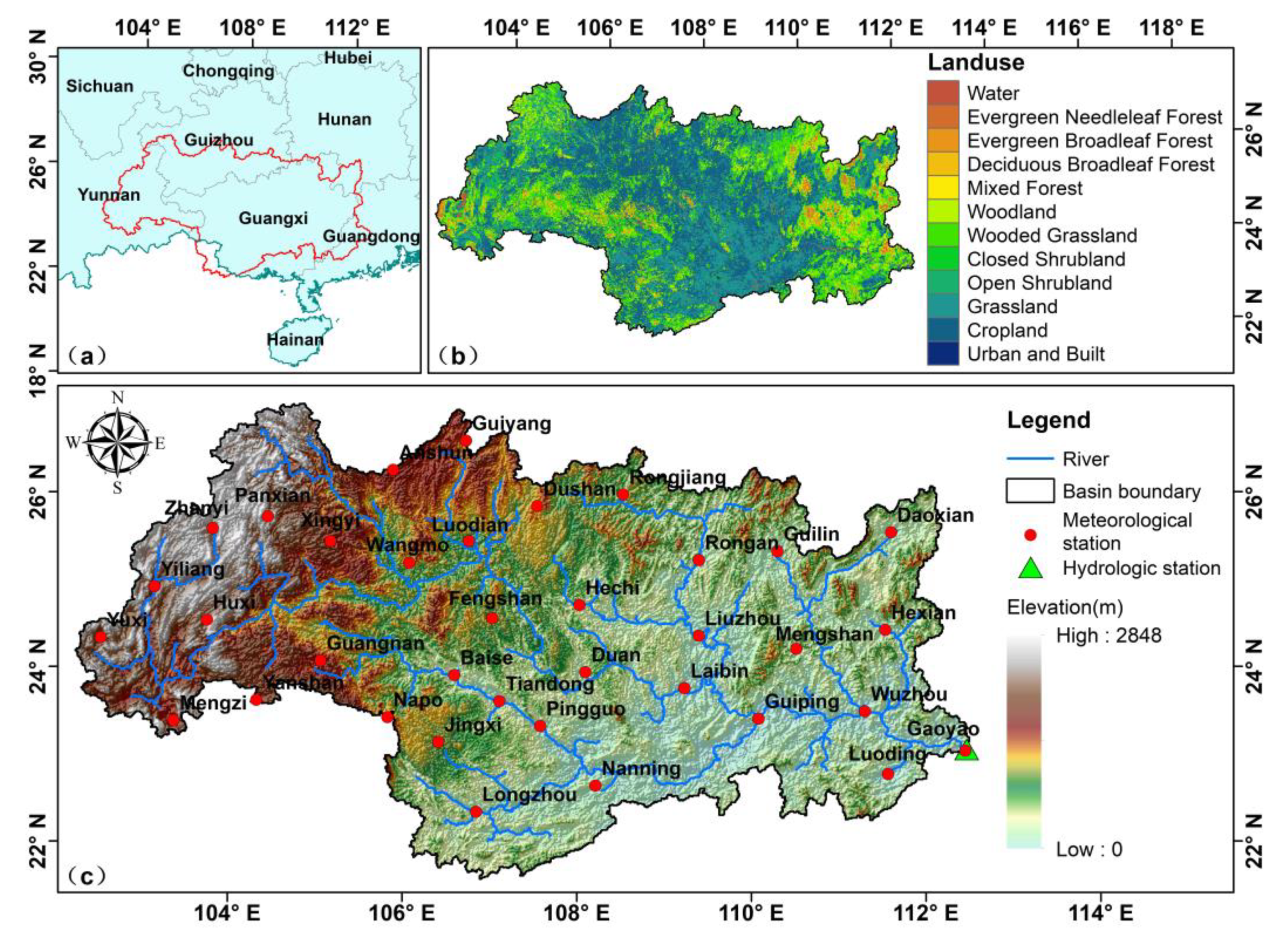
The Xijiang River Basin in southern China is located at 102°14’ E–114°50’ E, 21°31’ N–26°49’ N. It is the largest tributary of the Pearl River, accounting for 77.8% of total drainage area and 63.9% of the annual discharge of the entire Pearl (Figure 1c) [28,29]. It flows from upriver Yunnan Province through Guizhou Province, Guangxi Zhuang Autonomous Region (GZAR) and Guangdong Province (Figure 1a) [30]. The hydrological station of Gaoyao is the basin outlet. The total area of the basin extracted by ArcSWAT software is 368,451 km2. Twelve types of landuse were extracted from UMD land cover classification with a spatial resolution of one km (Figure 1b) [5]. They were water 0.61%, woodland 8.77%, wooded grassland 25.03%, grassland 23.35%, cropland 37.59%, urban and built 0.05%, respectively. The types of soil mainly included latosolic soil, red soil, and lime soil [31]. The basin belongs to a sub-tropical to tropical monsoon climate region [32]. Xijiang River has sufficient water resources with an average flow of 2.3 × 10¹¹ m3 year−1, only behind the Yangtze River in China [33]. It is the main source of water for agriculture, industrial water and 86 counties with a population of 300 million [28,34]. Historical records show that the largest flood of Xijiang River basin occurred at Wuzhou Station, which lasted about 30–40 days with an average peak flow of 57.8 billion m3/month [30]. Yujiang, Hongshuihe, Liujiang, Guijiang, Qianjiang, and Xunjiang are the main tributaries of the Xijiang River [35]. The precipitation of Xijiang River Basin is temporally variable, about 72% to 88% of precipitation takes place in the wet season from April to September [36,37]. In the cold season, its snow generally occurs in the mountainous regions of headwater of the west and the north [38]. The results of statistical calculation for 36 meteorological stations showed that mean annual precipitation is between 855.2 mm and 1908.9 mm. The maximum annual precipitation was 2807 mm, which happened at Guilin Station in 2002 and the minimum was 509.3 mm, which occurred at Mengzi Station in 1980. The annual average in precipitation, wind speed, temperature and relative humidity are 1346 mm, 1.8 m/s, 18.9 °C, and 77%, respectively. Spatially, the annual average precipitation decreases from coastal areas in the east to mountainous areas in the west [39]. In season, the precipitation of winter gets wetter and summer gets drier. Xijiang River Basin has a long history of development and is one of the most prosperous regions in China. With the increase of population, development of its industry and urbanization is rapid, and regional GDP (Gross Domestic Product) is 55.45% of the Guangxi total [40,41].
2.2. Data Series
In this study, daily precipitation from 1 January, 1960 to 31 December, 2008 was collected from 36 national standard meteorological stations in the Xijiang River Basin (Figure 1c and Table 1). The data were provided by National Meteorological Information Centre online database of the China Meteorological Administration (http://data.cma.cn/). Data from some stations were missing. We used an interpolation method called inverse distance weighted (IDW) to complement these missing data [42]. IDW is widely used in the geometric interpolation of precipitation, and it is demonstrated to be reliable and reasonable for the interpolation of precipitation [43,44,45,46,47]. IDW is mainly based on the following two assumptions: (1) The unsampled point is much more influenced by the nearby sampling point than those farther away, (2) the contribution of the sampled point to the unsampled point is proportional to the exponential power of the reciprocal of the distance between them. In this study, we also used IDW to interpolate daily precipitation with point-scale into raster data with spatial resolution of 0.25°, which was used for analysis of extreme precipitation in Xijiang River basin between 1960 and 2008. The raster precipitation is referred to as RPDI.
3. Research Methodology
In this study, the Mann–Kendall test (M-K) used to determine the variation trend of precipitation, which can indicate the increasing or decreasing trend of the detected time series in daily, monthly, seasonal, or annual time scales [48,49]. The advantage of this method is that the sample does not need to follow a certain distribution and is not interfered by a few abnormal values [11]. It is widely used to evaluate statistically significant trends in hydro-meteorological time series [6]. Moreover, it is a non-parametric test method recommended and widely used by the World Meteorological Organization (WMO) [50]. The magnitude of this trend change is calculated by Sen’s slope estimator (SSE) [12,51]. The concentration index (CI) and Lorenz asymmetry coefficient (LAC) were used to analyze the distribution and change of precipitation [6,12]. In recent years, the CI and LAC have been widely used to describe the uniformity of the annual and long-term distribution of meteorological elements in the fields of meteorology and hydrology [6,7,12,50,52]. The twelve extreme climate indices recommended by the Expert Team on Climate Change Detection and Indices (ETCCDI) were used to analyze the change for trend of daily extreme precipitation (Table 2) [11,13]. In Table 2, RR denotes daily precipitation and PRCP denotes precipitation. Wet days are defined as RR ≥ 1 mm, and dry days are defined as RR < 1 mm. Tan et al., [53] found that variations of precipitation intensity at different spatial locations within a basin have a significant impact on surface runoff and flood simulation. Thus, the probability density function (PDF) and the cumulative distribution function (CDF) were applied to analyze the frequent change of daily precipitation in the range of different precipitation intensity. The range of daily precipitation intensity was based on the classification standard of WMO [43,54]: 0 < P < 1 mm (tiny rain), 1 mm ≤ P < 2 mm (light rain), 2 mm ≤ P < 5 mm (low moderate rain), 5 mm ≤ P < 10 mm (high moderate rain), 10 mm ≤ P < 20 mm (low heavy rain), 20 mm ≤ P < 50 mm (high heavy rain), P ≥ 50 mm (violent rain). The season was divided as follows: Spring (March–May), Summer (June–August), Autumn (September–November), Winter (January–February, December). The maximum Lyapunov exponent (MLE) was used to qualitatively and quantitatively identify whether the system has chaotic characteristics [55]. In the process of constructing the chaotic system for daily precipitation: The delay time (τ) and the minimum embedding dimension (MED) were the most important parameters for calculating the Lyapunov exponent. The τ was calculated by the method called thee autocorrelation function (ACF) [56]. The MED was calculated by the method called Cao [57]. The MLE was calculated by the method called Wolf [55].
3.1. Mann–Kendall Trend Test
(1) H0:The time series are stable, independent and random, that is no trend;
(2) H1:The time series has an increasing or decreasing trend.
Under the assumption of H0, the text statistic S is defined as:
where sgn is a sign function, .
In Equation (1), when n ≥ 10, the statistic S follows a normal distribution. The standard Z is obtained after standardized calculation of S. It can be used as a test of significance. The standard Z is calculated according to the following equation:
when the time series has the same elements:
when the time series don’t have the same elements:
where n is the number of elements in the time series; m is the number of tied groups; ti is the number of elements in the ith group.
The Z is compared with the standard normal distribution table with two-tailed confidence levels (α = 0.01, α = 0.05, α = 0.1 and α = 0.2), when , the hypothesis H0 is accepted. Otherwise, the hypothesis H1 is accepted. At the 0.01, 0.05, 0.1, 0.2 significance levels, respectively equals to 2.576, 1.960, 1.645, 1.282 [6,11].
3.2. Concentration Index and Lorenz Asymmetry Coefficient
(1) The precipitation was sorted in an ascending order between 1960 and 2008, and a new time series was constructed;
(2) According to the size of the elements in , the appropriate i that was called classification interval was selected, the number of elements and the total amount of elements in each i were calculated. In this study, the classification interval i of the daily precipitation was determined to be one;
(3) The cumulative percentage of and were calculated based on the results of step (2);
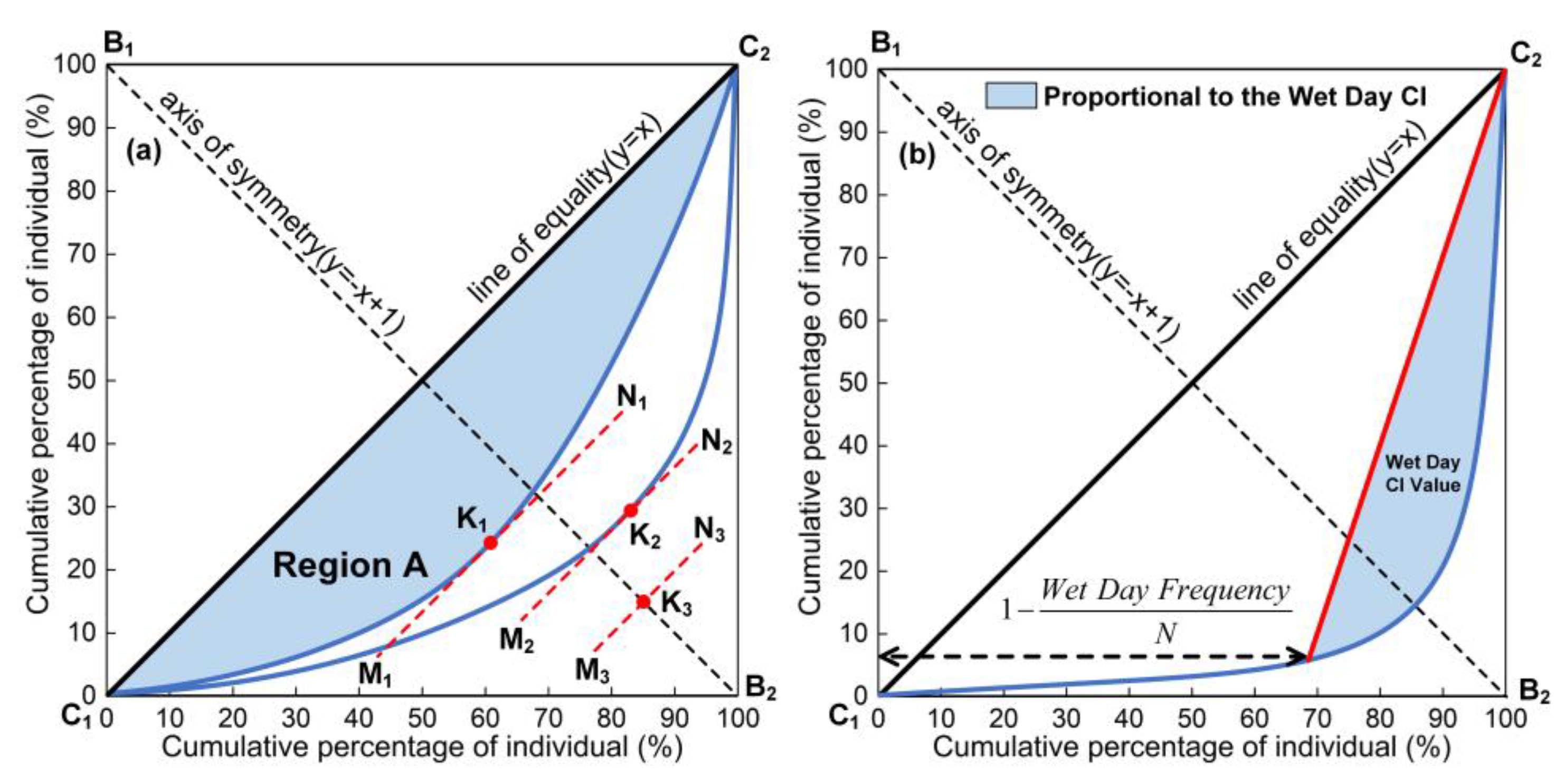
(4) Following step (3), cumulative percentages of precipitation days (X%) and cumulative percentages of precipitation amount (Y%) corresponding to each classification interval were fitted by an exponential curve (Equation (5)). The fitting curve Y was called the fitted Lorenz curve or the concentration curve (Figure 2).
(5) The was taken as an example for illustration. The area of region A surrounded by line of equality C1C2 and was calculated as follows:
The concentration index was calculated as follows
If annual precipitation were classified, the ACI was also calculated. If long-term precipitation from 1960 to 2008 were classified, the LCI was calculated. The CI has been widely used as a measure of inequality in precipitation distribution. A high CI indicates that homogeneity of precipitation distribution was very poor. We also studied the distribution of precipitation in wet days. The CI of the wet-day precipitation was defined as the area between the red line and the blue curve (the slash shadow region) (Figure 2b) [12,59]. When we compared the homogeneity of different data, they may have had the same CI [7]. In this case, the CI was not able to distinguish the differences between these concentration curves. In order to solve this deficiency, Damgaard et al. [60,61] proposed another index to describe the concentration curve called Lorenz asymmetry coefficient (LAC). For the time series ,the LAC was calculated according to the following equations:
where n is the number of elements in the ; is the average value of all elements; m is the number of elements less than ; is the qth element. When LAC < 1, the pointcut of the tangent line parallel to C1C2 on the concentration curve was below B1B2 (K1 in Figure 2) and illustrated that high concentration of precipitation occurred in a large number of low rainfall events. When LAC >1, the pointcut was above B1B2 (K2 in Figure 2) and illustrated that high concentration of precipitation occurred in a small number of very large rainfall events. The method was used to reveal the causes of precipitation with inhomogeneity distribution.
3.3. Reconstruction Parameter of Phase Space
Reconstructed phase space is the basis of analysis for chaotic time series. The calculation of the Lyapunov exponent is based on the vector in the reconstructed phase space. The delay time (τ) and embedding dimension (m) are the most important parameters in the reconstruction of phase space. The choice of the optimum τ is essential for geometrical and numerical analysis of reconstruction for the phase space [19]. The τ is the average length of memory of the system. In this study, for a scalar time series , the τ was calculated by ACF [21,56]. The formula is as follows:
where C(t) is the autocorrelation coefficient, t is the delay time, μ and σ is the mean and standard deviation of the time series, respectively. Observing the curve of the ACF, the delay time (τ) was equal to the corresponding t value when ACF dropped through the null point firstly.
(1) For a scalar time series , the delay time vectors can be reconstructed as follows:
where m is the embedding dimension; τ is the delay time is the ith reconstructed vector with embedding dimension m.
(2) Similar to the idea of the false neighbor method (FNN) [62], Cao [57] proposed the method of the averaged false nearest neighbors (AFN), AFN defines a quantity:
where ‖·‖ is measurement of Euclidian distance and is calculated by using the maximum norm; ; ; Fi(m+1) is the ith reconstructed vector with embedding dimension m+1; ; is the nearest neighbor of in the m-dimensional reconstructed phase space in the sense of distance ‖·‖.
(3) The mean value of a (i,m) is as follows:
To investigate the variation from m to m+1, we define:
If the time series has chaotic characteristics or comes from an attractor, E1(m) stops changing when m is greater than some .Then is the minimum embedding dimension. Otherwise, E1(m) will not attain a saturated value. Since available samples are limited, random time series may happen that the E1(m) stops changing at some m. Therefore, we defined E2(m), which is used to distinguish whether a set of data is deterministic or random [57,62].
For random data, E2(m) will be equal to one for any m in this case. However, for deterministic data, E2(m) cannot be a constant for any m or must exist some m such that E2(m) ≠ 1. Therefore, if a time series has deterministic data, it must satisfy both conditions of E1(m) and E2(m). Only deterministic data have chaotic characteristics.
3.4. The Maximum Lyapunov Exponent (MLE)
Both the saturated correlation dimension (SCD) and MLE can be used to judge the existence of chaos and intensity of chaotic characteristics for dynamical systems [55,63]. For the method of SCD, it is difficult to find a consistent region or scaling region of LogC(r)/Log(r) and there are some errors that the correlation exponent are calculated by the least square method [19]. Therefore, we used MLE that is calculated by the method called Wolf to quantitatively determine whether the system had chaotic characteristics in this study [55]. If MLE < 0, it indicates that the time series is no chaotic characteristic. If MLE = 0, it indicates that the time series is in a critical state. If MLE > 0 or larger, it indicates that the chaotic characteristics is larger. In this study, the MLE was computed from the following equations [55]:
(1) The (in the Section 3.3) was also called a phase point on the phase space. We regarded as the initial phase point or vector. For the , the range of evolutive time t was from 0 to M (M = N−(m−1)τ−1). Then we calculated the maximum (dmax), minimum (dmin) and average (davg) distance between any two phase points in . The distance between the evolutionary phase point and the current phase point was defined as follows:
where is the threshold of distance; k, k1, k2 is assigned as 0.02, 0.5, 2; the and is the maximum and minimum limit of the distance between the evolutionary point of the searching and current point.
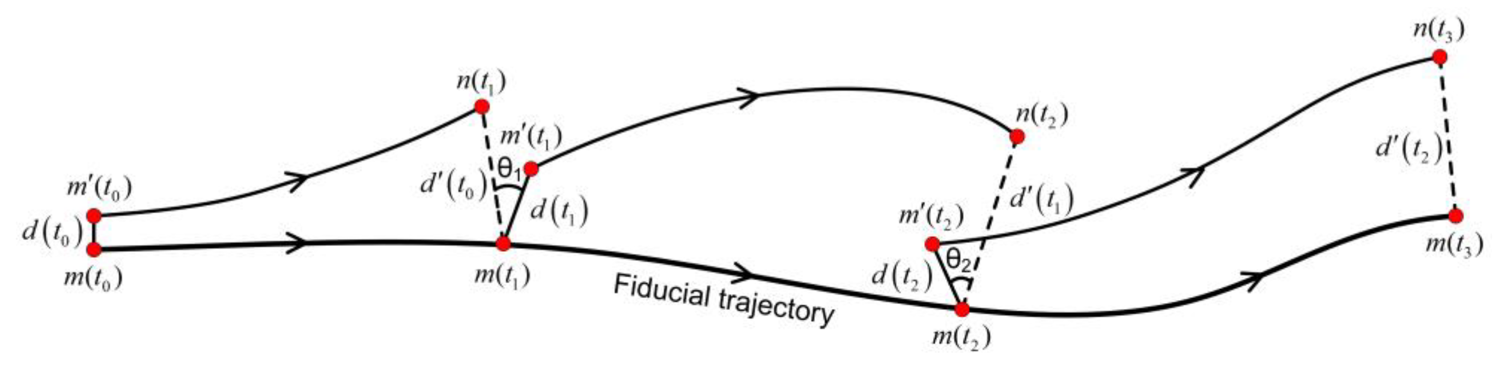
(2) In Figure 3, the initial phase point is taken as the fiducial point, is the phase point with the minimum distance from · is the initial nearest distance and . P is the position difference between the evolutionary phase point and the current phase point. If the current phase point is i, the evolutionary phase point will be limited to a brief separation and it can only be searched in the phase point of . In this study, P was taken as the average period of the time series calculated by the fast Fourier transform (FFT). The evolution step of time (t) was taken as 1.Firstly, was evolved to along the fiducial trajectory and was evolved to . Then we needed to find a new point which satisfies two conditions: The distance from point was small and the angle was as small as possible. If no point satisfied the above conditions, the search range of the distance was increased to find a new point again. The calculation method of the angle was as follows:
The initial minimum threshold of was 45°, which will decrease with the increase of evolution time.
(3) Step (2) was calculated repeatedly until the end of evolution time. The MLE was calculated as follows:
4. Results
4.1. Spatiotemporal Variations of Precipitation in the Xijiang River Basin between 1960 and 2008
4.1.1. Temporary Distribution of Precipitation in Monthly and Seasonal Scales
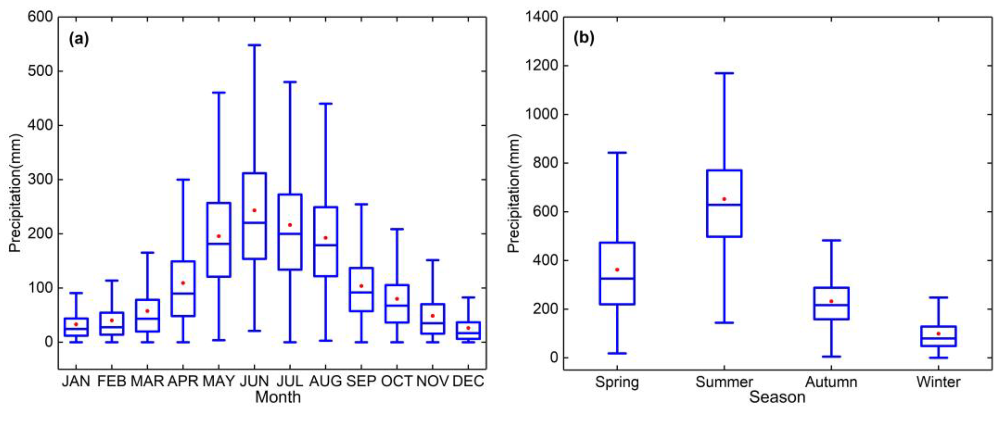
Figure 4 showed that the mean and median distribution of monthly precipitation was similar to the normal distribution and had symmetry. The maximum of the average value was located in June of summer, which was 243.4 mm, and the median was 220.3 mm. The minimum value of the average was located in December of winter, which was 26.2 mm and the median was 16.8 mm. The maximum difference of precipitation between the upper and lower third quartile occurred in June, which was 527.4 mm. When the daily precipitation was greater than or equal to 0.1 mm, we think that there was precipitation occurring. The larger monthly precipitation occurred in May, June, July and August. The days of their average annual precipitation was 17, 18, 18 and 18, respectively. The average monthly precipitation was the largest in June. For quarterly precipitation, the median and mean of summer were the largest, which was 628.8 mm and 652.4 mm respectively. The median and mean of the winter were the least, which was 80 mm and 99.2 mm respectively.
4.1.2. Inhomogeneity of Spatial Distribution for Monthly Precipitation
Table 3 shows that R2 (Coefficient of Determination) was close to 1 and RMSE (Root Mean Squared Error) was low, which shows that the concentration curve can express the trend of Lorenz Curve. The |Z| of stations were lower. The range of variation was between –0.688 and 1.617, and had no significant change at the significance level of 0.05. SSE and Z had the same symbols, which show the same trend of change. SSE was also lower, the range of change was between –1.24% and 2.3%, which indicated that change of the monthly precipitation was relatively stable, there were no significant trends of increase or decrease. LCI was between 0.407 and 0.528. The largest LCI occurred at Baise station, but its LAC was not the maximum. The maximum value of LAC occurred at Rongan station, which was 0.936. LAC was between 0.79 and 0.936, which is less than 1. They were located in the south and north of the middle of the basin, respectively. The results indicate that inhomogeneity of monthly precipitation is caused by in a large number of low rainfall events.
4.1.3. Inhomogeneity of Spatial Distribution for Daily Precipitation
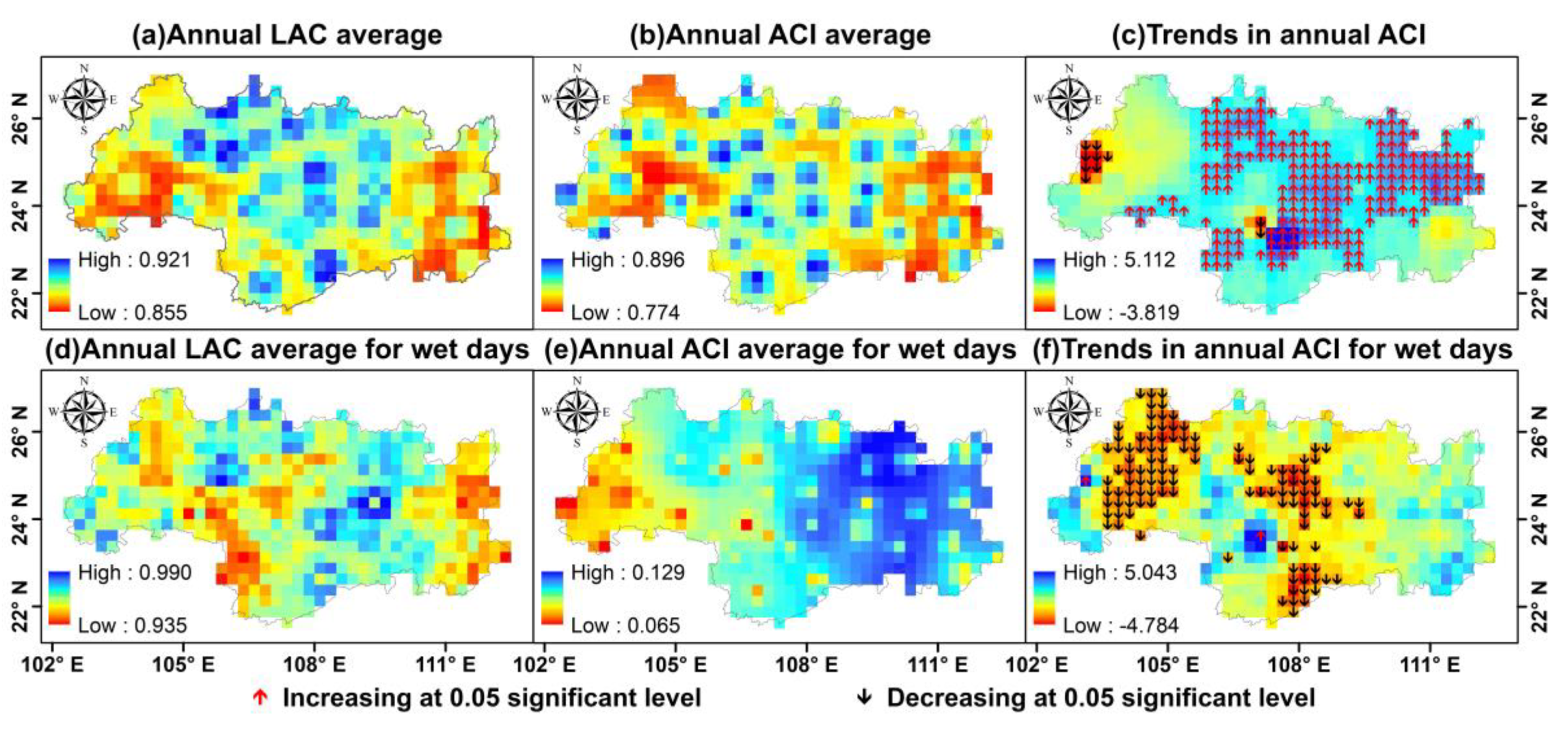
Figure 5 shows the change of LAC and ACI for annual daily precipitation in the Xijiang River Basin. We used RPDI to calculate the average values of ACI, LAC and the trend of ACI at the 0.05 significance level between 1960 and 2008, respectively. The CI was highly sensitive to precipitation of wet days. Thus, we also analyzed the uniformity of precipitation in wet days. The LAC was between 0.855 and 0.921, LAC and ACI were smaller in the west and east of the basin, ACI was between 0.744 and 0.896, indicating that the distribution of daily precipitation was very uneven and precipitation was mainly concentrated in a large number of low rainfall events. The trend of ACI was mostly positive, with positive and negative values accounting for 92.2% and 7.6% respectively, which indicates that precipitation becomes more and more uneven. The proportion of grids with significant increase and decrease was 41% and 1.9%, respectively. The middle and north of the basin showed a significant increase, and a few number of grids in the west showed a significant decrease. In the wet days, LAC was close to 1 and ACI was close to 0, which showed that the distribution of precipitation was uniform. ACI was larger in the east and smaller in the west. ACI showed a significant decreasing trend at most of the grids in the middle and west, indicating that the precipitation distribution was becoming more uniform. The proportion of positive and negative trends were 7.4% and 92.4%, respectively. The proportion of rasters with significant decrease was 22%.
4.1.4. Characteristics and Trend in Frequency and Cumulative Distribution of Daily Precipitation
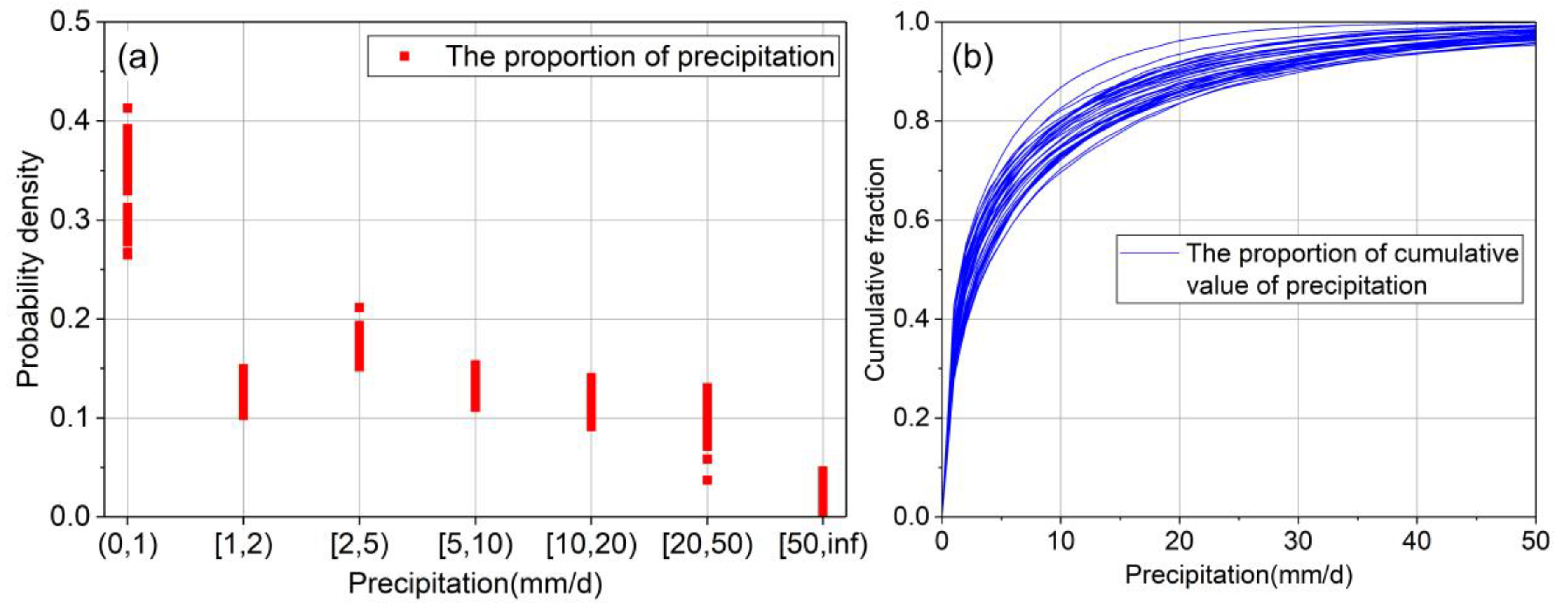
In terms of flood disaster and risk management, more than a certain level of flood can cause damage to life and property, destruction of infrastructure, serious losses of industry and agriculture, and so on. Intensity and duration of precipitation are important indicators of flood occurrence. Figure 6 shows the following: (1) The proportion of precipitation in different intervals of precipitation intensity for meteorological stations; and the (2) cumulative distribution function of precipitation less than 50 mm/d. The largest proportion was tiny rain, between 33.5% and 41.3%. Its maximum and minimum occurred at Yanshan and Guiping, respectively. The minimum proportion was violent rain, between 0.1% and 4.7%. Its maximum and minimum occur at Duan and Yanshan, respectively. The proportion of high heavy rain at Yanshan station was also the minimum, which was 3.7%. The mean proportion of precipitation for each precipitation intensity interval was 33.5%, 12.4%, 17.5%, 13.2%, 11.5%, 9.4%, and 2.5%, respectively. Duan has the highest frequency for violent rain, and the probability of disasters caused by extreme precipitation near the station is the highest. Therefore, it is necessary to improve the forecasting ability of this region for extreme weather. The cumulative distribution function showed different rates of change. At 10 mm/d, 20 mm/d and 50 mm/d, the range of change for cumulative values was [69.7%, 86.8%], [83.6%, 96.2%] and [95.4%, 99.9%], respectively. When the precipitation was more than 50 mm/d, the cumulative value was close to 1. The curve with the fastest change with cumulative fraction occurred at Yanshan; the proportion of its tiny rain was the largest.
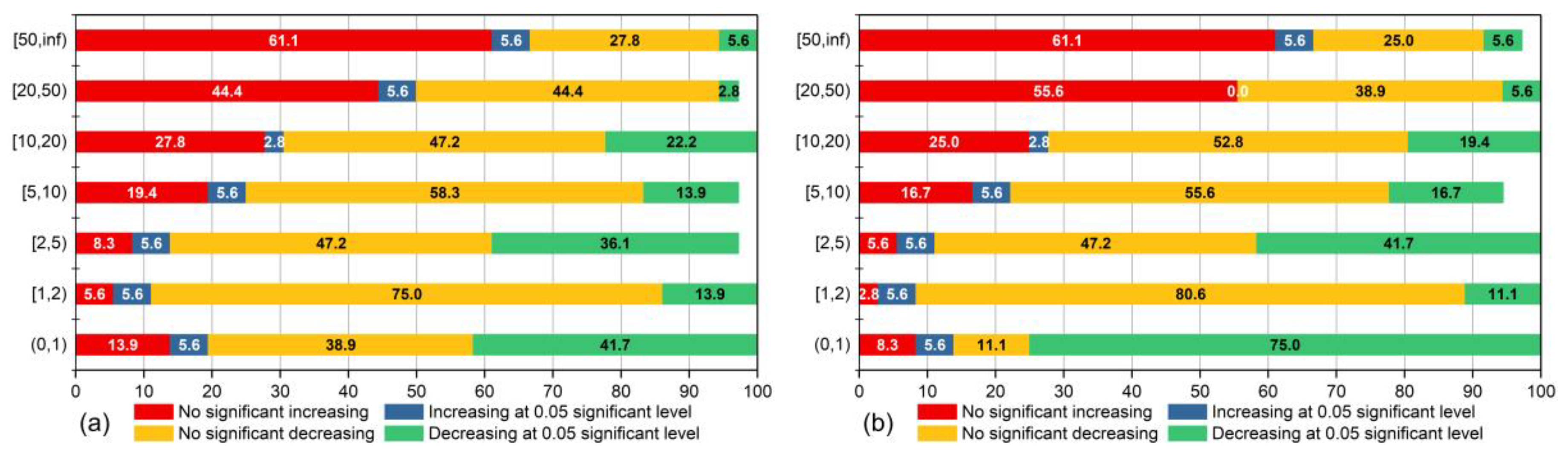
Figure 7 shows that the trend of precipitation and precipitation events for station in seven classification intervals at a 0.05 significant level. Figure 7a indicates that between light rain and violent rain, as the interval increased, the proportion of stations with "no significant increasing" increased also. Except for low heavy rain, the proportion of other intervals with "increasing at 0.05 significant level" was 5.6%. Nearly half of the station for tiny rain were decreasing, the proportion was 41.7%. The proportion of increase or decrease for violent rain was 5.6%. The precipitation days of high heavy rain do not exist for significant stations.
4.1.5. Spatial Variation of Extreme Precipitation Events
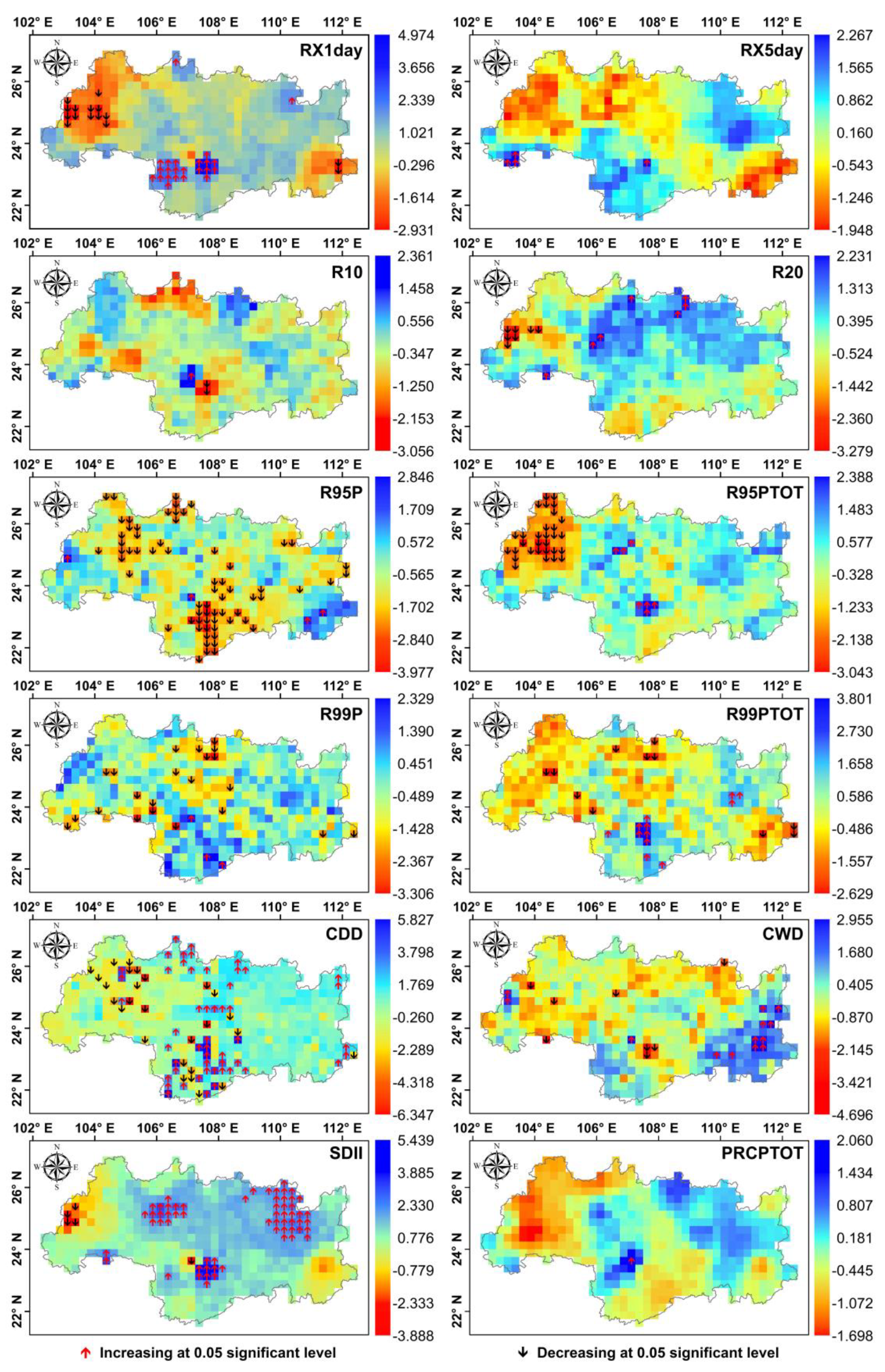
Figure 8 shows the trend of the extreme precipitation index in the Xijiang River Basin. Max one-day precipitation amount (RX1day) and max 5-day precipitation amount (RX5day) show a decreasing trend in the northwest and southeast of the basin. RX1day shows a significant decrease in some areas of the northwest, while RX5day does not show a significant decrease. This RX1day had a significant increase in the south. The rate of change for RX1day and RX5day was [−0.67 mm/year, 1.20 mm/year] and [−0.62 mm/year, 1.12 mm/year], respectively. The rates of change for the number of precipitation >= 10 mm days (R10) and the number of precipitation >= 20 mm days (R20) were stable, and there was a significant change in a few number of grids. The rates of change for R10 and R20 were [−0.25 days/year, 0.19 days/year] and [−0.14 days/year, 0.11 days/year], respectively. R20 shows an increasing trend in the northeast. R95P and R99P showed a decreasing trend in most of the grids. The rate of change for R95P was [−0.08 mm/year, 0.06 mm/year], and the rate of change for R99P was 0 mm/year. R95P shows a significant decrease in the south and northwest of the basin. The negative rates of change for R95P and R99P accounted for 76.9% and 62%, respectively. Precipitation on very wet days (R95PTOT) and precipitation on extremely wet days (R99PTOT) showed a decreasing trend in the northwest of the basin, and some grids of R95PTOT showed a significant decreasing trend. The rates for these were [−2.08mm/year, 1.94 mm/year] and [−1.71 mm/year, 1.76mm/year], respectively. In the middle and northwest of the basin, consecutive dry days (CDD) showed a significant increase or decrease in different degrees. In the southeast, consecutive wet days (CWD) of some grids showed a significant increase. The rates of change for CDD and CWD were [−0.52 days/year, 0.45 days/year] and [−0.23 days/year, 0.14 days/year], respectively. Some grids of the simple daily intensity index (SDII) showed a significant increase in the middle and northeast, the rate of change was [−0.07 mm/year, 0.03 mm/year]. The PRCPTOT showed a decreasing trend in the northwest, and its rate of change was [−3.04, 4.04]. In conclusion, although the CDD showed significant increases at some grids, others also showed significant decreases. The extreme precipitation index related to precipitation and precipitation frequency showed a decreasing trend in different degrees. Therefore, there may be a risk of drought in the west of the basin in the future, and precipitation in other locations is still relatively abundant.
4.2. Study on Its Chaotic Characteristics of Precipitation in the Xijiang River Basin between 1989 and 2008
The chaotic identification and characteristic of dynamic systems for meteorology need to be established in the reconstructed phase space. Therefore, the reconstructed phase space is the basis for chaotic analysis and research of all meteorological elements. If τ is large, the number of vectors in the reconstructed phase space will be reduced and the adjacent orbits will be deviated. All relevant information for reconstructed phase space is lost. If τ is too small, the phase orbit of the reconstructed dynamical system will be squeezed in the diagonal line, and the dynamical characteristics of the system will not be fully displayed. If m is too large, the calculation time of will be increased, the length of data will be reduced, and the points in the phase space will be too sparse. If m is too small, the number of attractors needed for the research system will not be accommodated [19,22,64,65,66,67]. The length of time series should be reasonable. When the Lyapunov exponent is calculated by G-P method, m is determined by the slope of logC(r)-logr curve with the steady change. If the length of the data is small, the slope of the steady change will become difficult to determine [18,67]. In this study, the Wolf method was used by us to calculate the MLE [55]. For this, the sample must meet the following conditions: (1) The number of phase points need to provide enough number of replacement points on the fiducial trajectory; (2) the number of trajectories of data need probe stretching (but not folding) within the attractor; (3) the number of data points per orbit that allow for proper attractor reconstruction with evolution coordinates [55] (Figure 3). The length of the time series was chosen from 1989 to 2008, which not only meets the requirement of the Wolf method, but also improves the reliability of the results and reduces the time of calculation. MED and MLB were calculated by the server, which takes about seven days approximately.
4.2.1. Determination of Delay Time
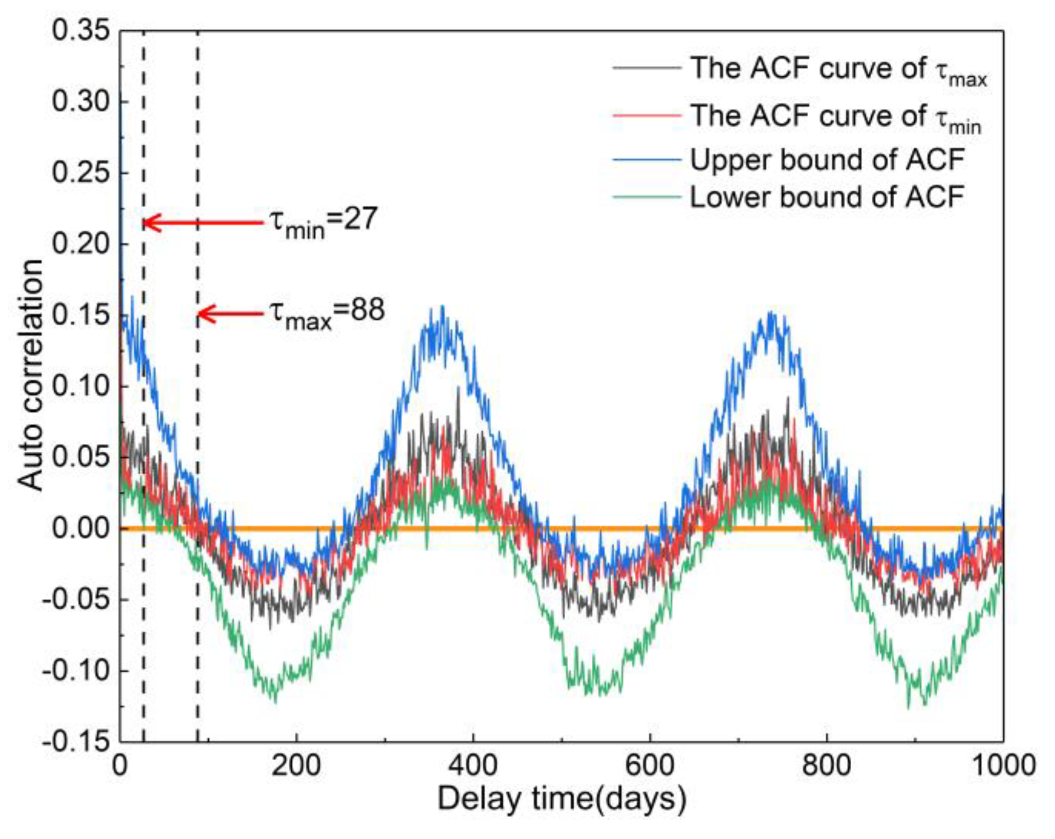
Figure 9 shows the ACF curve of daily precipitation for meteorological stations in the Xijiang River Basin. The maximum length of τ was set to 1000. The period of this curve is about 365. The τ is the corresponding time when the ACF curve firstly passes the null point. The maximum of τ occurred at Mengzi station, which was 88. The minimum of τ occurred at Daoxian Station, which was 77. The average value of τ was 70. The autocorrelation coefficient near the null point varied greatly, and its value was between −0.1264 and 0.3065.
4.2.2. Determination of Minimum Embedding Dimension
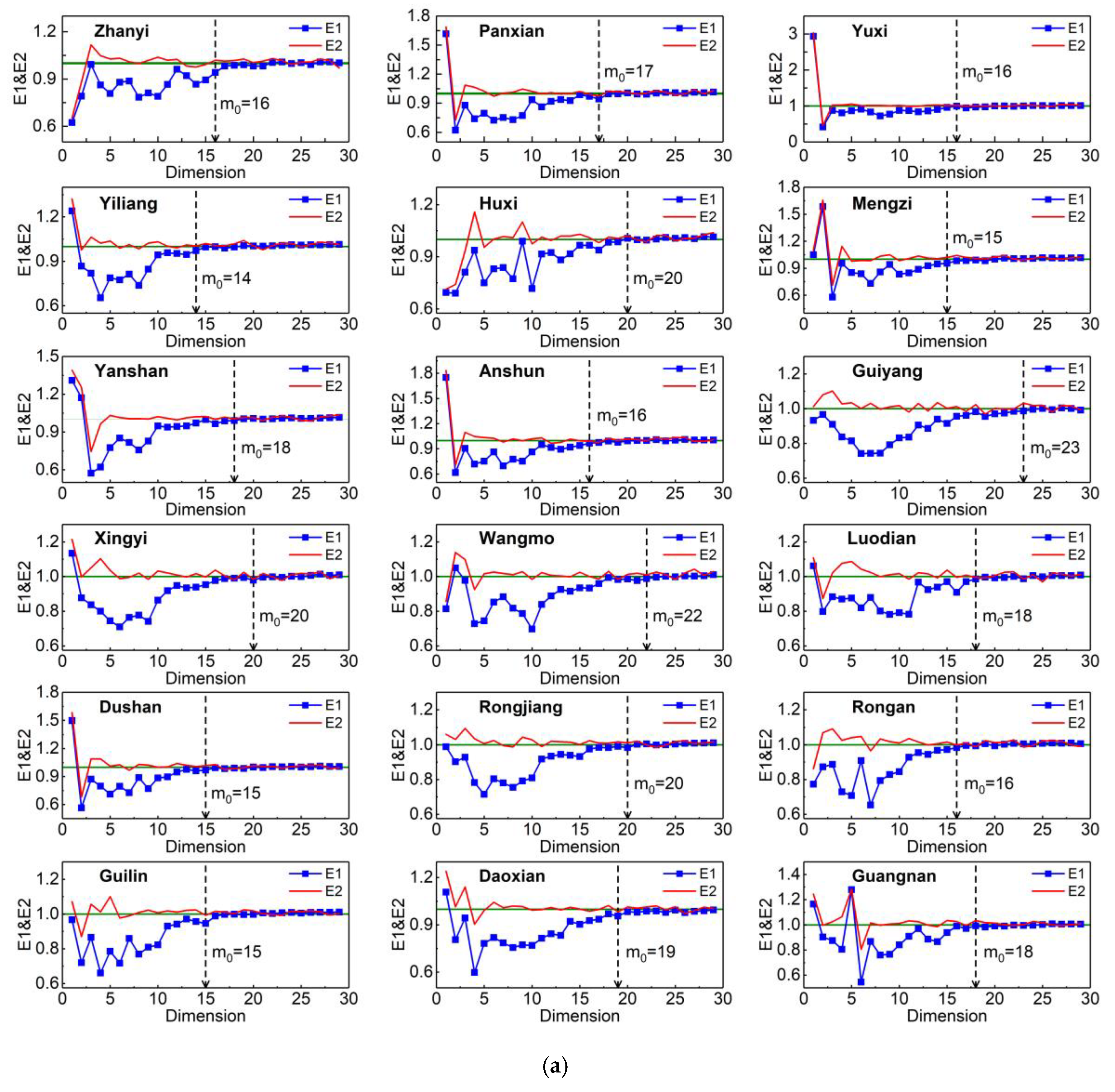
In this study, the MED was computed by the Cao method [57]. This method was chosen mainly for the following reasons: (1) The Cao has no empirical parameter and does not strongly depends on the length of sample; and (2) for particular data, it may have the same effect as deterministic data. Cao is able to distinguish between deterministic data and random data. Figure 10 shows the variation curves of E1 and E2 for meteorological stations. For the calculation length of m, the Pingguo station was set to 40, and the other stations were set to 30. Because it is difficult to determine the critical point () of the stable change of E1 and E2 curves for Pingguo when was set to 30, we increased to 40. Figure 10a,b show that there are some m values such that E2 was not equal to 1. Therefore, the type of the data for all meteorological stations was deterministic. Initially, the E1 curve changed significantly when m was small. With increasing of m, the E1 value increased gradually. Finally, the trend became stable when , was the minimum embedding dimension. The result of MED was between 11 and 30, with an average value of 19.
4.2.3. Identification and Spatial Variation of Chaos Characteristics
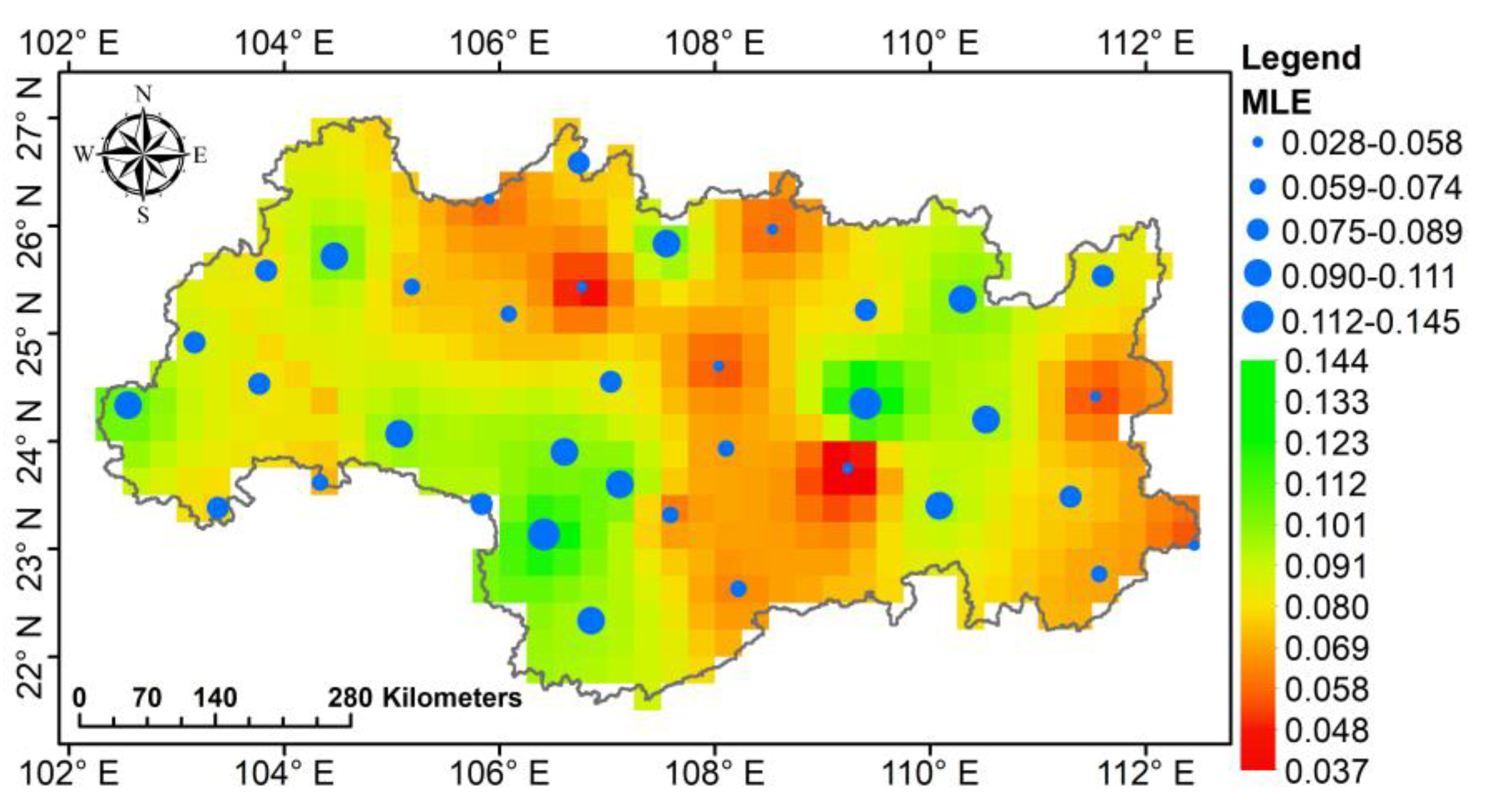
Figure 11 shows the MLE of meteorological stations and spatial distribution of MLE obtained by IDW. The MLE of all stations was greater than zero, and daily precipitation of Xijiang River Basin was proved to be chaotic. There were deterministic components in this time series. The maximum and minimum of chaotic intensity occurred in Liuzhou and Laibin stations, and MLEs were 0.144 and 0.028, respectively. Compared with others, their elevation and annual precipitation average were both smaller (Table 1). The average value of MLE was 0.0816, and the MLE was smaller in the middle and east of the basin.
5. Discussion
5.1. Variation Analysis of Conventional Precipitation and Extreme Precipitation
In this study, we analyzed the homogeneity and trend of monthly precipitation over the long period on a point scale, and homogeneity and trend of annual daily precipitation for all days and wet days over the short period on a spatial scale between 1960 and 2008. Finally, the spatial variation of the extreme precipitation index was analyzed. Interestingly, Figure 4 and Caloiero et al., [68] shows the opposite trend for seasonal and monthly precipitation. Due to the influence of the geographical location and its mountainous features, the climatic feature of Calabria was highly opposite. had a good fitting effect on data points, R2 was close to one (Table 3). The fitted exponential curve used in this study can completely represent the variation of the Lorenz curve. This fitting effect also occured in the study of Shi et al., [6] and Zheng et al., [7]. The maximum LCI occurred at Baise Station, but its LAC was not the maximum. The maximum of LAC occurred at Rongan Station, which was different from the result of Shi et al., [6], the maximum of which for LCI and LAC occurred at the same station. Figure 5 shows that the precipitation of all days and wet days was concentrated in a large number of low rainfall events. There were great differences with variation of their homogeneity. The proportions of wet days and all days which tended to be evenly distributed was 92.4% and 7.6%, respectively. In many studies, the threshold of judging extreme precipitation for ETCCDI was based on the method of traditional percentile [1,2,4,11,12,14,69,70]. This method assumes that precipitation is subject to a uniform distribution, but actually it is not so, and its regularity is poor. Therefore, we refer to the method of Luo et al., [71] when calculating the threshold. In the case that considering the actual probability distribution of precipitation, this data was transformed into a standard normal distribution and then restored. The rationality and accuracy of calculation for the threshold were improved. Many studies show that there is a significant increase with extreme precipitation from April to September in China, especially in the northwest and southeast [2]. Wang et al., [72] indicated that extreme precipitation shows significantly variation in the western and southern region of china. Sun et al., [12] indicated that annual precipitation of the Loess Plateau shows a non-significant negative trend over the last fifty years. Halimatou et al., [13] indicated that evidence for increases in the frequency of both heavy rains and severe droughts in many regions of the world, it shows a wide range of regional differences. Croitoru et al., [4] indicated that more extreme precipitation events have occurred over large areas of land especially in the midland high-latitude regions. Zhang et al., [73] indicated that extreme precipitation events have increased in western and southeast China since 1950. Zhao et al., [74] indicated that extreme precipitation events are also increasing and show apparent spatial differences in China. Zheng et al., [7] indicated that annual and seasonal rainfall show no significant changes in the Pearl River Basin. Zhang et al., [75] indicated that uneven distribution of precipitation occurs in the flood and drought stages of the basin. Wu et al., [76] indicated that extreme precipitation has a significant increase in the Tarim River Basin. Results of the above research indicated that the extreme precipitation shows different changes for frequency, intensity and distribution in many regions of the world. Table 4 shows that comparison of trends in extreme precipitation indices from this and other studies. In our research, the R99PTOT increases at an average rate of 0.06 mm/year, while the R95PTOT decreases at a rate of −0.01 mm/year, which indicating an increase in precipitation between R95PTOT and R99PTOT. Meanwhile, the extreme precipitation of Xijiang River Basin has the same trend as China, northwest China and Georgia. R95P decreases with −0.006days/year, which has the opposite trend compared with China and the world. The Xijiang is the largest tributary of the Pearl River. In addition to CWD and R95P, other indices have the same trend as Pearl River Basin. In the spatial analysis of extreme precipitation, many studies do not interpolate the precipitation of stations, but interpolate the index. This method is not accurate. It ignores the complex spatial variability of precipitation with the change of time. Therefore, the results of interpolation for indices at different locations are quite different from those of real ones.
5.2. Vertification of Chaotic Characteristics for Daily Precipitation Time Series Near the Coastal Areas
The study shows that there are different degrees of chaos at the stations and spatial scales across the Xijiang River Basin (Figure 11). Compared with MED of Dhanya et al., [21], Dhanya et al., [22], Sivakumar et al., [23] and Jayawardena et al., [65], our research has a very high value, which is between 11 and 33. Compared with Mohammad et al., [77], the MED and MLE is both larger. The MLE is between 0.037 and 0.144, while MLE of Mohammad is only between 6 × 10⁻⁵ and 4 × 10⁻⁴. In a word, the precipitation shows high dimension and high chaos characteristics.
6. Conclusions
This paper studies the spatiotemporal variation and chaotic characteristics of precipitation across the Xijiang River Basin. The main conclusions of this study are as follows:
- (1)
- LAC and ACI are smaller in the west and east of the basin. Precipitation tends to be unevenly distributed with time, which is mainly concentrated in a large number of low rainfall events on wet days, precipitation of the middle and west is more and more uniform.
- (2)
- Duan station has the highest frequency for Violent rain, and the probability of disasters caused by extreme precipitation near the station is the highest. Seventy five percent of the stations for tiny rain days show "decreasing at 0.05 significant level". The curve with the fastest change with cumulative fraction occurs at Yanshan.
- (3)
- There may be a risk of drought on the west of the basin in the future, and precipitation in other locations is still relatively abundant. The average rates of variation for RX1_day, RX5_day, SD_II, R10, R20, CDD, CWD, R95P, R99P, R95PTOT, R99PTOT, PRCPTOT are 0.093 mm/year, 0.035 mm/year, 0.013 mm/year, −0.016 days/year, 0.009 days/year, 0.029 days/year, 0.001 days/year, −0.006 days/year, 0 days/year, −0.01 mm/year, 0.063 mm/year, −0.308 mm/year, respectively.
- (4)
- This daily precipitation has been proved to have high dimension and high chaotic characteristics. The MLE is smaller in the middle and east of the basin. The maximum and minimum of chaotic intensity occur in Liuzhou and Laibin station, and MLE are 0.144 and 0.028, respectively.
Author Contributions
X.D. completed the statistical analysis and wrote the paper; W.L., H.W. and X.L. provided the writing ideas and supervised the study; W.Z. and Z.Y. was responsible for study designing and modifying the language.
Funding
This research was supported by National Key R & D Program of China (2017YFB0203104), the National Natural Science Fund (51709273) and Science and Technology Innovation Project for Water Conservancy in Guangdong Province (2017-06).
Conflicts of Interest
The authors declare that there are no conflicts of interests regarding the publication of this paper.
References
- Santos, M.; Fragoso, M.; Santos, J.A. Regionalization and susceptibility assessment to daily precipitation extremes in mainland Portugal. Appl. Geogr. 2017, 86, 128–138. [Google Scholar] [CrossRef]
- Gao, L.; Huang, J.; Chen, X.; Chen, Y.; Liu, M. Contributions of natural climate changes and human activities to the trend of extreme precipitation. Atmos. Res. 2018, 205, 60–69. [Google Scholar] [CrossRef]
- Ipcc, C.W.T. Climate Change 2007: Mitigation. Contribution of Working Group III to the Fourth Assessment Report of the Intergovernmental Panel on Climate Change. Comput. Geom. 2007, 18, 95–123. [Google Scholar]
- Croitoru, A.E.; Chiotoroiu, B.C.; Ivanova Todorova, V.; Toricǎ, V. Changes in precipitation extremes on the Black Sea Western Coast. Glob. Planet. Chang. 2013, 102, 10–19. [Google Scholar] [CrossRef]
- Hansen, M.C.; Defries, R.S.; Townshend, J.R.G.; Sohlberg, R. Global land cover classification at 1km spatial resolution using a classification tree approach. Int. J. Remote Sens. 2000, 21, 1331–1364. [Google Scholar] [CrossRef]
- Shi, W.; Yu, X.; Liao, W.; Wang, Y.; Jia, B. Spatial and temporal variability of daily precipitation concentration in the Lancang River basin, China. J. Hydrol. 2013, 495, 197–207. [Google Scholar] [CrossRef]
- Zheng, Y.; He, Y.; Chen, X. Spatiotemporal pattern of precipitation concentration and its possible causes in the Pearl River basin, China. J. Clean. Prod. 2017, 161, 1020–1031. [Google Scholar] [CrossRef]
- Some’e, B.S.; Ezani, A.; Tabari, H. Spatiotemporal trends and change point of precipitation in Iran. Atmos. Res. 2012, 113, 1–12. [Google Scholar]
- Gao, T.; Wang, H.J.; Zhou, T. Changes of extreme precipitation and nonlinear influence of climate variables over monsoon region in China. Atmos. Res. 2017, 197, 379–389. [Google Scholar] [CrossRef]
- Sharma, C.S.; Panda, S.N.; Pradhan, R.P.; Singh, A.; Kawamura, A. Precipitation and temperature changes in eastern India by multiple trend detection methods. Atmos. Res. 2016, 180, 211–225. [Google Scholar] [CrossRef]
- Tang, X.; Miao, C.; Xi, Y.; Duan, Q.; Lei, X.; Li, H. Analysis of precipitation characteristics on the loess plateau between 1965 and 2014, based on high-density gauge observations. Atmos. Res. 2018, 213, 264–274. [Google Scholar] [CrossRef]
- Sun, Q.; Miao, C.; Duan, Q.; Wang, Y. Temperature and precipitation changes over the Loess Plateau between 1961 and 2011, based on high-density gauge observations. Glob. Planet. Chang. 2015, 132, 1–10. [Google Scholar] [CrossRef]
- Halimatou, A.T.; Kalifa, T.; Kyei-Baffour, N. Assessment of changing trends of daily precipitation and temperature extremes in Bamako and Ségou in Mali from 1961–2014. Weather Clim. Extrem. 2017, 18, 8–16. [Google Scholar] [CrossRef]
- Khoi, D.N.; Trang, H.T. Analysis of Changes in Precipitation and Extremes Events in Ho Chi Minh City, Vietnam. Procedia Eng. 2016, 142, 229–235. [Google Scholar] [CrossRef] [Green Version]
- Jakob, D.; Walland, D. Variability and long-term change in Australian temperature and precipitation extremes. Weather Clim. Extrem. 2016, 14, 36–55. [Google Scholar] [CrossRef] [Green Version]
- Huang, G.; Wen, G.H. Spatial and temporal variations of light rain events over China and the mid-high latitudes of the Northern Hemisphere. Sci. Bull. 2013, 58, 1402–1411. [Google Scholar] [CrossRef] [Green Version]
- Rohwer, R. Order out of Chaos: Man’s New Dialogue with Nature. Phys. Bull. 1986, 37, 11. [Google Scholar] [CrossRef]
- Sivakumar, B. Chaos theory in hydrology: Important issues and interpretations. J. Hydrol. 2000, 227, 1–20. [Google Scholar] [CrossRef]
- Ng, W.W.; Panu, U.S.; Lennox, W.C. Chaos based Analytical techniques for daily extreme hydrological observations. J. Hydrol. 2007, 342, 17–41. [Google Scholar] [CrossRef]
- Ghorbani, M.A.; Khatibi, R.; Mehr, A.D.; Asadi, H. Chaos-based multigene genetic programming: A new hybrid strategy for river flow forecasting. J. Hydrol. 2018, 562, 455–467. [Google Scholar] [CrossRef]
- Dhanya, C.T.; Kumar, D.N. Nonlinear ensemble prediction of chaotic daily rainfall. Adv. Water Resour. 2010, 33, 327–347. [Google Scholar] [CrossRef]
- Dhanya, C.T.; Kumar, D.N. Multivariate nonlinear ensemble prediction of daily chaotic rainfall with climate inputs. J. Hydrol. 2011, 403, 292–306. [Google Scholar] [CrossRef]
- Sivakumar, B.; Berndtsson, R.; Olsson, J.; Jinno, K. Evidence of chaos in the rainfall-runoff process. Hydrol. Sci. J. 2001, 46, 131–145. [Google Scholar] [CrossRef]
- Jothiprakash, V. Chaotic analysis of daily rainfall series in Koyna reservoir catchment area, India. Stoch. Environ. Res. Risk Assess. 2013, 27, 1371–1381. [Google Scholar] [CrossRef]
- Li, Y.; Fang, K.; Cao, C.; Li, D.; Gan, Z. A tree-ring chronology spanning the past 210 years in the coastal area of Southeast China and its relationship with climate change. Clim. Res. 2016, 67, 209–220. [Google Scholar] [CrossRef]
- Sadatzki, H.; Sarnthein, M.; Andersen, N. Changes in monsoon-driven upwelling in the South China Sea over glacial Terminations I and II: A multi-proxy record. Int. J. Earth Sci. 2016, 105, 1273–1285. [Google Scholar] [CrossRef]
- Fischer, T.; Gemmer, M.; Liu, L.; Su, B. Change-points in climate extremes in the Zhujiang River Basin, South China, 1961–2007. Clim. Chang. 2012, 110, 783–799. [Google Scholar] [CrossRef]
- Li, C.; Li, S.-L.; Yue, F.-J.; Liu, J.; Zhong, J.; Yan, Z.-F.; Zhang, R.-C.; Wang, Z.-J.; Xu, S. Identification of sources and transformations of nitrate in the Xijiang River using nitrate isotopes and Bayesian model. Sci. Total Environ. 2019, 646, 801–810. [Google Scholar] [CrossRef]
- Sun, H.; Han, J.; Li, D.; Zhang, S.; Lu, X. Chemical weathering inferred from riverine water chemistry in the lower Xijiang basin, South China. Sci. Total Environ. 2010, 408, 4749–4760. [Google Scholar] [CrossRef]
- Niu, J.; Sivakumar, B.; Chen, J. Impacts of increased CO2 on the hydrologic response over the Xijiang (West River) basin, South China. J. Hydrol. 2013, 505, 218–227. [Google Scholar] [CrossRef]
- Xu, Z.; Liu, C.-Q. Water geochemistry of the Xijiang basin rivers, South China: Chemical weathering and CO2 consumption. Appl. Geochem. 2010, 25, 1603–1614. [Google Scholar] [CrossRef]
- Niu, J.; Chen, J.; Sun, L. Exploration of drought evolution using numerical simulations over the Xijiang (West River) basin in South China. J. Hydrol. 2015, 526, 68–77. [Google Scholar] [CrossRef]
- Lin, Q.; Wu, Z.; Singh, V.P.; Sadeghi, S.H.R.; He, H.; Lu, G. Correlation between hydrological drought, climatic factors, reservoir operation, and vegetation cover in the Xijiang Basin, South China. J. Hydrol. 2017, 549, 512–524. [Google Scholar] [CrossRef]
- Liu, Y.; Peng, P.; Li, X.; Zhang, S.; Ren, M. Polychlorinated dibenzo-p-dioxins and dibenzofurans (PCDD/Fs) in water and suspended particulate matter from the Xijiang River, China. J. Hazard. Mater. 2008, 152, 40–47. [Google Scholar] [CrossRef] [PubMed]
- Lei, X.; Zhang, J.; Wang, H.; Wang, M.; Khu, S.-T.; Li, Z.; Tan, Q. Deriving mixed reservoir operating rules for flood control based on weighted non-dominated sorting genetic algorithm II. J. Hydrol. 2018, 564, 967–983. [Google Scholar] [CrossRef]
- Yao, G.; Gao, Q.; Wang, Z.; Huang, X.; He, T.; Zhang, Y.; Jiao, S.; Ding, J. Dynamics Of CO2 partial pressure and CO2 outgassing in the lower reaches of the Xijiang River, a subtropical monsoon river in China. Sci. Total Environ. 2007, 376, 255–266. [Google Scholar] [CrossRef]
- Zhang, G.; Bai, J.; Xiao, R.; Zhao, Q.; Jia, J.; Cui, B.; Liu, X. Heavy metal fractions and ecological risk assessment in sediments from urban, rural and reclamation-affected rivers of the Pearl River Estuary, China. Chemosphere 2017, 184, 278–288. [Google Scholar] [CrossRef]
- Yuan, F.; Zhao, C.; Jiang, Y.; Ren, L.; Shan, H.; Zhang, L.; Zhu, Y.; Chen, T.; Jiang, S.; Yang, X.; et al. Evaluation on uncertainty sources in projecting hydrological changes over the Xijiang River basin in South China. J. Hydrol. 2017, 554, 434–450. [Google Scholar] [CrossRef]
- Liu, B.; Chen, J.; Chen, X.; Lian, Y.; Wu, L. Uncertainty in determining extreme precipitation thresholds. J. Hydrol. 2013, 503, 233–245. [Google Scholar] [CrossRef]
- Liu, Z.; Zhao, M.; Sun, H.; Yang, R.; Chen, B.; Yang, M.; Zeng, Q.; Zeng, H. “Old” carbon entering the South China Sea from the carbonate-rich Pearl River Basin: Coupled action of carbonate weathering and aquatic photosynthesis. Appl. Geochem. 2017, 78, 96–104. [Google Scholar] [CrossRef]
- Dang, L.; Xu, Y.; Tang, Q. The pattern of available construction land along the Xijiang River in Guangxi, China. Land Use Policy 2015, 42, 102–112. [Google Scholar] [CrossRef]
- Bartier, P.M.; Keller, C.P. Multivariate interpolation to incorporate thematic surface data using inverse distance weighting (IDW). Comput. Geosci. 1996, 22, 795–799. [Google Scholar] [CrossRef]
- Tuo, Y.; Duan, Z.; Disse, M.; Chiogna, G. Evaluation of precipitation input for SWAT modeling in Alpine catchment: A case study in the Adige river basin (Italy). Sci. Total Environ. 2016, 573, 66–82. [Google Scholar] [CrossRef] [PubMed] [Green Version]
- Garcia, M.; Peters-Lidard, C.D.; Goodrich, D.C. Spatial interpolation of precipitation in a dense gauge network for monsoon storm events in the southwestern United States. Water Resour. Res. 2008, 44, 781–782. [Google Scholar] [CrossRef]
- Liu, X.D.; Yin, Z.Y. Spatial and temporal variation of summer precipitation over the eastern Tibetan Plateau and the North Atlantic oscillation. J. Clim. 2001, 14, 2896–2909. [Google Scholar] [CrossRef]
- Nalder, I.A.; Wein, R.W. Spatial interpolation of climatic Normals: Test of a new method in the Canadian boreal forest. Agric. For. Meteorol. 1998, 92, 211–225. [Google Scholar] [CrossRef]
- Tong, K.; Su, F.; Yang, D.; Hao, Z. Evaluation of satellite precipitation retrievals and their potential utilities in hydrologic modeling over the Tibetan Plateau. J. Hydrol. 2014, 519, 423–437. [Google Scholar] [CrossRef]
- Pakalidou, N.; Karacosta, P. Study of very long-period extreme precipitation records in Thessaloniki, Greece. Atmos. Res. 2018, 208, 106–115. [Google Scholar] [CrossRef] [Green Version]
- Mann, H.B. Nonparametric test against trend. Econometrica 1945, 13, 245–259. [Google Scholar] [CrossRef]
- Deng, S.; Li, M.; Sun, H.; Chen, Y.; Qu, L.; Zhang, X. Exploring temporal and spatial variability of precipitation of Weizhou Island, South China Sea. J. Hydrol. Reg. Stud. 2017, 9, 183–198. [Google Scholar] [CrossRef]
- Sen, P.K. Estimates of the Regression Coefficient Based on Kendall’s Tau. J. Am. Stat. Assoc. 1968, 63, 1379–1389. [Google Scholar] [CrossRef]
- Sanguesa, C.; Pizarro, R.; Ibanez, A.; Pino, J.; Rivera, D.; Garcia-Chevesich, P.; Ingram, B. Spatial and Temporal Analysis of Rainfall Concentration Using the Gini Index and PCI. Water 2018, 10, 112. [Google Scholar] [CrossRef]
- Tan, M.L.; Ibrahim, A.L.; Duan, Z.; Cracknell, A.P.; Chaplot, V. Evaluation of Six High-Resolution Satellite and Ground-Based Precipitation Products over Malaysia. Remote Sens. 2015, 7, 1504–1528. [Google Scholar] [CrossRef] [Green Version]
- Duan, Z.; Liu, J.; Tuo, Y.; Chiogna, G.; Disse, M. Evaluation of eight high spatial resolution gridded precipitation products in Adige Basin (Italy) at multiple temporal and spatial scales. Sci. Total Environ. 2016, 573, 1536–1553. [Google Scholar] [CrossRef] [PubMed] [Green Version]
- Wolf, A.; Swift, J.B.; Swinney, H.L.; Vastano, J.A. Determining Lyapunov exponents from a time series. Phys. D Nonlinear Phenom. 1985, 16, 285–317. [Google Scholar] [CrossRef] [Green Version]
- Yang, X.-H.; Mei, Y.; She, D.-X.; Li, J.-Q. Chaotic Bayesian optimal prediction method and its application in hydrological time series. Comput. Math. Appl. 2011, 61, 1975–1978. [Google Scholar] [CrossRef] [Green Version]
- Cao, L.Y. Practical method for determining the minimum embedding dimension of a scalar time series. Phys. D 1997, 110, 43–50. [Google Scholar] [CrossRef]
- Douglas, E.M.; Vogel, R.M.; Kroll, C.N. Trends in floods and low flows in the United States: Impact of spatial correlation. J. Hydrol. 2000, 240, 90–105. [Google Scholar] [CrossRef]
- Rajah, K.; O’Leary, T.; Turner, A.; Petrakis, G.; Westra, S. Changes to the temporal distribution of daily precipitation. Geophys. Res. Lett. 2015, 41, 8887–8894. [Google Scholar] [CrossRef]
- Masaki, Y.; Hanasaki, N.; Takahashi, K.; Hijioka, Y. Global-scale analysis on future changes in flow regimes using Gini and Lorenz asymmetry coefficients. Water Resour. Res. 2014, 50, 4054–4078. [Google Scholar] [CrossRef]
- Damgaard, C.; Weiner, J. Describing inequality in plant size or fecundity. Ecology 2000, 81, 1139–1142. [Google Scholar] [CrossRef]
- Kedra, M. Deterministic chaotic dynamics of Raba River flow (Polish Carpathian Mountains). J. Hydrol. 2014, 509, 474–503. [Google Scholar] [CrossRef]
- Grassbeger, P.; Procaccia, I. Characterization of strange attractors. Phys. Rev. Lett. 1983, 50, 346. [Google Scholar] [CrossRef]
- Havstad, J.W.; Ehlers, C.L. Attractor dimension of nonstationary dynamical systems from small data sets. Phys. Rev. A 1989, 39, 845–853. [Google Scholar] [CrossRef] [PubMed]
- Jayawardena, A.W.; Lai, F. Analysis and prediction of chaos in rainfall and stream flow time series. J. Hydrol. 1994, 153, 23–52. [Google Scholar] [CrossRef]
- Schreiber, T.; Kantz, H. Observing and Predicting Chaotic Signals: Is 2% Noise Too Much? Springer: Berlin/Heidelberg, Germany, 1996; ISBN 978-3-642-80254-6. [Google Scholar]
- Procaccia, I. Measuring the strangeness of strange attractors. Phys. D Nonlinear Phenom. 1983, 9, 189–208. [Google Scholar]
- Caloiero, T.; Coscarelli, R.; Ferrari, E.; Sirangelo, B. Trends in the daily precipitation categories of Calabria (southern Italy). Procedia Eng. 2016, 162, 32–38. [Google Scholar] [CrossRef]
- Manton, M.J.; Della-Marta, P.M.; Haylock, M.R.; Hennessy, K.J.; Nicholls, N.; Chambers, L.E.; Collins, D.A.; Daw, G.; Finet, A.; Gunawan, D. Trends in extreme daily rainfall and temperature in Southeast Asia and the South Pacific: 1961–1998. Int. J. Climatol. 2010, 21, 269–284. [Google Scholar] [CrossRef]
- Mei, C.; Liu, J.; Chen, M.-T.; Wang, H.; Li, M.; Yu, Y. Multi-decadal spatial and temporal changes of extreme precipitation patterns in northern China (Jing-Jin-Ji district, 19602013–). Quat. Int. 2018, 476, 1–13. [Google Scholar] [CrossRef]
- Luo, M.; Xiong, S.; Liang, Y.; Bureau, Y.M.; Bureau, C.M. Comparative study of calculated threshold values in regional extreme precipitation. J. Meteorol. Sci. 2013, 33, 549–554. [Google Scholar]
- Wang, X.; Hou, X.; Wang, Y. Spatiotemporal variations and regional differences of extreme precipitation events in the Coastal area of China from 1961 to 2014. Atmos. Res. 2017, 197, 94–104. [Google Scholar] [CrossRef]
- Zhang, Q.; Li, J.; Singh, V.P.; Xu, C.-Y. Copula-based spatio-temporal patterns of precipitation extremes in China. Int. J. Climatol. 2013, 33, 1140–1152. [Google Scholar] [CrossRef]
- Zhao, Y.; Zou, X.; Cao, L.; Xu, X. Changes in precipitation extremes over the Pearl River Basin, southern China, during 1960–2012. Quat. Int. 2014, 333, 26–39. [Google Scholar] [CrossRef]
- Zhang, Q.; Gu, X.; Singh, V.P.; Xiao, M.; Xu, C.-Y. Flood frequency under the influence of trends in the Pearl River basin, China: Changing patterns, causes and implications. Hydrol. Process. 2015, 29, 1406–1417. [Google Scholar] [CrossRef]
- Wu, X.; Wang, Z.; Zhou, X.; Lai, C.; Lin, W.; Chen, X. Observed changes in precipitation extremes across 11 basins in China during 1961–2013. Int. J. Climatol. 2016, 36, 2866–2885. [Google Scholar] [CrossRef]
- Zounemat-Kermani, M.; Kisi, O. Time series analysis on marine wind-wave characteristics using chaos theory. Ocean Eng. 2015, 100, 46–53. [Google Scholar] [CrossRef]
- Sun, W.; Mu, X.; Song, X.; Wu, D.; Cheng, A.; Qiu, B. Changes in extreme temperature and precipitation events in the Loess Plateau (China) during 1960–2013 under global warming. Atmos. Res. 2016, 168, 33–48. [Google Scholar] [CrossRef]
- Wang, B.; Zhang, M.; Wei, J.; Wang, S.; Li, S.; Ma, Q.; Li, X.; Pan, S. Changes in extreme events of temperature and precipitation over Xinjiang, northwest China, during 1960–2009. Quat. Int. 2013, 298, 141–151. [Google Scholar] [CrossRef]
- Wang, B.; Zhang, M.; Wei, J.; Wang, S.; Li, X.; Li, S.; Zhao, A.; Li, X.; Fan, J. Changes in extreme precipitation over Northeast China, 1960–2011. Quat. Int. 2013, 298, 177–186. [Google Scholar] [CrossRef]
- Song, X.; Song, S.; Sun, W.; Mu, X.; Wang, S.; Li, J.; Li, Y. Recent changes in extreme precipitation and drought over the Songhua River Basin, China, during 1960–2013. Atmos. Res. 2015, 157, 137–152. [Google Scholar] [CrossRef]
- Li, Y.-G.; He, D.; Hu, J.-M.; Cao, J. Variability of extreme precipitation over Yunnan Province, China 1960–2012. Int. J. Climatol. 2015, 35, 245–258. [Google Scholar] [CrossRef]
- Keggenhoff, I.; Elizbarashvili, M.; Amiri-Farahani, A.; King, L. Trends in daily temperature and precipitation extremes over Georgia, 1971–2010. Weather Clim. Extrem. 2014, 4, 75–85. [Google Scholar] [CrossRef]
- Omondi, P.A.; Awange, J.L.; Forootan, E.; Ogallo, L.A.; Barakiza, R.; Girmaw, G.B.; Fesseha, I.; Kululetera, V.; Kilembe, C.; Mbati, M.M.; et al. Changes in temperature and precipitation extremes over the Greater Horn of Africa region from 1961 to 2010. Int. J. Climatol. 2014, 34, 1262–1277. [Google Scholar] [CrossRef]
Figure 1.
Distribution map of the study area of Xijiang River Basin. (a) China’s provinces in the Xijiang River Basin; (b) distribution map of landuse; (c) distribution map of meteorological stations, hydrologic stations and elevation.
Figure 1.
Distribution map of the study area of Xijiang River Basin. (a) China’s provinces in the Xijiang River Basin; (b) distribution map of landuse; (c) distribution map of meteorological stations, hydrologic stations and elevation.

Figure 2.
(a) Concentration curve of precipitation distribution. There are three types: One symmetric curve () and two asymmetric curves ( and ); (b) concentration curve of precipitation in wet days (PRCP ≥ 1 mm) [6,59].

Figure 3.
Schematic of evolution and replacement procedure of neighbor points when calculating the largest Lyapunov exponent by Wolf.
Figure 3.
Schematic of evolution and replacement procedure of neighbor points when calculating the largest Lyapunov exponent by Wolf.

Figure 4.
Boxplots of the precipitation for 36 meteorological stations in 1960–2008. (a) Monthly precipitation distribution; (b) seasonal precipitation distribution. Red dots represent the mean of precipitation.
Figure 4.
Boxplots of the precipitation for 36 meteorological stations in 1960–2008. (a) Monthly precipitation distribution; (b) seasonal precipitation distribution. Red dots represent the mean of precipitation.

Figure 5.
The average values and trends of ACI and LAC for annual all days and wet days in 1960–2008.
Figure 5.
The average values and trends of ACI and LAC for annual all days and wet days in 1960–2008.

Figure 6.
Statistical function of precipitation for 36 meteorological stations in the Xijiang River Basin between 1960 and 2008. (a) Probability density function; (b) cumulative distribution function. Square dots filled with red represent probability density.
Figure 6.
Statistical function of precipitation for 36 meteorological stations in the Xijiang River Basin between 1960 and 2008. (a) Probability density function; (b) cumulative distribution function. Square dots filled with red represent probability density.

Figure 7.
Results of the Mann–Kendall trend test of daily precipitation classification for 36 meteorological stations. (a) The annual precipitation falling within each classification interval. (b) The total numbers of daily precipitation events falling within each classification interval every year. The X axis represents that percentages of meteorological stations with the same trend of change (increasing or decreasing, significant increasing or decreasing at a 0.05 level).

Figure 8.
Spatial variability of trends for the extreme precipitation indices in the Xijiang River Basin between 1960 and 2008. At a 0.05 level, the upward red or downward black arrow indicates that this trend is increasing or decreasing significantly, respectively.
Figure 8.
Spatial variability of trends for the extreme precipitation indices in the Xijiang River Basin between 1960 and 2008. At a 0.05 level, the upward red or downward black arrow indicates that this trend is increasing or decreasing significantly, respectively.

Figure 9.
Autocorrelation function plot (lag length up to 1000 days) of daily precipitation for 36 meteorological stations.
Figure 9.
Autocorrelation function plot (lag length up to 1000 days) of daily precipitation for 36 meteorological stations.

Figure 10.
(a) E1 and E2 curves of 36 meteorological stations in the Xijiang River Basin calculated by the Cao method. is the critical point of steady change. (b) E1 and E2 curves of 36 meteorological stations in the Xijiang River Basin calculated by Cao method. is the minimum embedding dimension.
Figure 10.
(a) E1 and E2 curves of 36 meteorological stations in the Xijiang River Basin calculated by the Cao method. is the critical point of steady change. (b) E1 and E2 curves of 36 meteorological stations in the Xijiang River Basin calculated by Cao method. is the minimum embedding dimension.


Figure 11.
Spatial distribution of the largest Lyapunov exponent across Xijiang River Basin between 1989 and 2008.
Figure 11.
Spatial distribution of the largest Lyapunov exponent across Xijiang River Basin between 1989 and 2008.


Table 1.
Information on the meteorological stations which were collected in this study.
| Station Code | Name | Longitude (°) | Latitude (°) | Elevation (m) | Annual Precipitation Average (1960–2008) (mm) | Durations with Missing Data |
|---|---|---|---|---|---|---|
| 56786 | Zhanyi | 103.83 | 25.58 | 1898.7 | 995.9 | Nm |
| 56793 | Panxian | 104.47 | 25.72 | 1800 | 1390.6 | Nm |
| 56875 | Yuxi | 102.55 | 24.33 | 1716.9 | 916.9 | Nm |
| 56880 | Yiliang | 103.17 | 24.92 | 1532.1 | 929.4 | 1968.01.01–1968.04.30 1991.06.01–2006.12.31 |
| 56886 | Huxi | 103.77 | 24.53 | 1704.3 | 923.8 | Nm |
| 56985 | Mengzi | 103.38 | 23.38 | 1300.7 | 855.2 | Nm |
| 56991 | Yanshan | 104.33 | 23.62 | 1561.1 | 1359.4 | 1960.01.01–2001.12.31 |
| 57806 | Anshun | 105.90 | 26.25 | 1431.1 | 1307.2 | Nm |
| 57816 | Guiyang | 106.73 | 26.58 | 1223.8 | 1287.3 | Nm |
| 57902 | Xingyi | 105.18 | 25.43 | 1378.5 | 1651.3 | Nm |
| 57906 | Wangmo | 106.08 | 25.18 | 566.8 | 1012.8 | 1960.06.28 |
| 57916 | Luodian | 106.77 | 25.43 | 440.3 | 1343.1 | Nm |
| 57922 | Dushan | 107.55 | 25.83 | 1013.3 | 1115.7 | Nm |
| 57932 | Rongjiang | 108.53 | 25.97 | 285.7 | 1347.6 | Nm |
| 57947 | Rongan | 109.40 | 25.22 | 121.3 | 1246.4 | 1968.02.01–1968.02.29 |
| 57957 | Guilin | 110.30 | 25.32 | 164.4 | 1151.7 | Nm |
| 57965 | Daoxian | 111.60 | 25.53 | 192.2 | 1327.3 | Nm |
| 59007 | Guangnan | 105.07 | 24.07 | 1249.6 | 1199.3 | 1967.08.01–1968.12.31 |
| 59021 | Fengshan | 107.03 | 24.55 | 484.6 | 1908.9 | 1968.02.01–1968.03.31 |
| 59023 | Hechi | 108.03 | 24.70 | 211 | 1883.3 | Nm |
| 59037 | Duan | 108.10 | 23.93 | 170.8 | 1514.2 | Nm |
| 59046 | Liuzhou | 109.40 | 24.35 | 96.8 | 1040.5 | Nm |
| 59058 | Mengshan | 110.52 | 24.20 | 145.7 | 1529.6 | Nm |
| 59065 | Hexian | 111.53 | 24.42 | 108.8 | 1496.2 | Nm |
| 59209 | Napo | 105.83 | 23.42 | 794.1 | 1724.4 | Nm |
| 59211 | Baise | 106.60 | 23.90 | 173.5 | 1453.0 | Nm |
| 59218 | Jingxi | 106.42 | 23.13 | 739.9 | 1740.9 | 1968.01.28–1968.02.01 |
| 59224 | Tiandong | 107.12 | 23.60 | 111.2 | 1548.5 | 1988.01.01–2006.12.31 |
| 59228 | Pingguo | 107.58 | 23.32 | 108.8 | 1389.4 | 1960.01.01–1987.12.31 |
| 59242 | Laibin | 109.23 | 23.75 | 84.9 | 1097.9 | Nm |
| 59254 | Guiping | 110.08 | 23.40 | 42.5 | 1635.2 | Nm |
| 59265 | Wuzhou | 111.30 | 23.48 | 114.8 | 1256.9 | Nm |
| 59278 | Gaoyao | 112.45 | 23.03 | 41 | 1340.6 | Nm |
| 59417 | Longzhou | 106.85 | 22.33 | 128.8 | 1352.1 | Nm |
| 59431 | Nanning | 108.22 | 22.63 | 121.6 | 1710.6 | Nm |
| 59462 | Luoding | 111.57 | 22.77 | 53.3 | 1473.9 | Nm |
“Nm” indicates that daily precipitation of the meteorological station is no missing during the period of study.
Table 2.
List of twelve extreme precipitation indices used in this study.
| Index Name | Description | Definition | Unit |
|---|---|---|---|
| RX1day | Max 1-day precipitation amount | Annual maximum 1-day precipitation | mm |
| RX5day | Max 5-day precipitation amount | Annual maximum consecutive 5-day precipitation | mm |
| SDII | Simple daily intensity index | Annual total precipitation divided by the number of wet days in the year | mm/day |
| R10 | Number of precipitation >= 10 mm days | Annual count of days when daily precipitation (RR) >= 10 mm | days |
| R20 | Number of precipitation >= 20 mm days | Annual count of days when RR >= 20 mm | days |
| CDD | Consecutive dry days | Maximum number of consecutive days with RR < 1 mm | days |
| CWD | Consecutive wet days | Maximum number of consecutive days with RR >= 1 mm | days |
| R95P | Very wet days | Number of days when RR > 95th percentile of precipitation on wet days | days |
| R99P | Extremely wet days | Number of days when RR > 99th percentile of precipitation on wet days | days |
| R95PTOT | Precipitation in very wet days | Annual total precipitation (PRCP) when RR > 95th percentile in wet days | mm |
| R99PTOT | Precipitation in extremely wet days | Annual total PRCP when RR > 99th percentile in wet days | mm |
| PRCPTOT | Annual total wet-day precipitation | Annual total PRCP in wet days | mm |
Table 3.
Values for coefficient of determination (R2), root-mean-square error (RMSE), Z, Sen’s slope estimator (SSE), LCI and Lorenz asymmetry coefficient (LAC) statistics of monthly precipitation for 36 meteorological stations across Xijiang River basin (1960–2008).
Table 3.
Values for coefficient of determination (R2), root-mean-square error (RMSE), Z, Sen’s slope estimator (SSE), LCI and Lorenz asymmetry coefficient (LAC) statistics of monthly precipitation for 36 meteorological stations across Xijiang River basin (1960–2008).
| Station Name | R2 | RMSE | Z | SSE | LCI | LAC | Station Name | R2 | RMSE | Z | SSE | LCI | LAC |
|---|---|---|---|---|---|---|---|---|---|---|---|---|---|
| Zhanyi | 0.9998 | 0.0056 | −0.066 | −0.07% | 0.515 | 0.813 | Fengshan | 0.9994 | 0.0079 | 0.639 | 1.03% | 0.522 | 0.827 |
| Panxian | 0.9996 | 0.0069 | 0.025 | 0.02% | 0.518 | 0.801 | Hechi | 0.9995 | 0.0070 | −0.175 | −0.30% | 0.488 | 0.897 |
| Yuxi | 0.9996 | 0.0075 | 0.434 | 0.42% | 0.515 | 0.830 | Duan | 0.9993 | 0.0084 | −0.379 | −0.75% | 0.513 | 0.898 |
| Yiliang | 0.9996 | 0.0074 | 0.903 | 0.87% | 0.513 | 0.808 | Liuzhou | 0.9992 | 0.0093 | −0.061 | −0.13% | 0.475 | 0.892 |
| Huxi | 0.9997 | 0.0060 | −0.656 | −0.63% | 0.510 | 0.833 | Mengshan | 0.9993 | 0.0085 | −0.290 | −0.64% | 0.461 | 0.892 |
| Mengzi | 0.9997 | 0.0067 | 0.426 | 0.41% | 0.497 | 0.849 | Hexian | 0.9995 | 0.0073 | −0.312 | −0.60% | 0.438 | 0.873 |
| Yanshan | 0.9996 | 0.0079 | −0.268 | −0.30% | 0.474 | 0.812 | Napo | 0.9998 | 0.0056 | −0.324 | −0.45% | 0.520 | 0.822 |
| Anshun | 0.9999 | 0.0029 | −0.619 | −0.79% | 0.510 | 0.866 | Baise | 0.9998 | 0.0043 | 0.129 | 0.15% | 0.528 | 0.864 |
| Guiyang | 0.9997 | 0.0054 | −0.406 | −0.49% | 0.480 | 0.860 | Jingxi | 0.9998 | 0.0045 | 0.574 | 1.06% | 0.509 | 0.822 |
| Xingyi | 0.9997 | 0.0054 | −0.362 | −0.50% | 0.505 | 0.859 | Tiandong | 0.9999 | 0.0031 | 1.617 | 2.30% | 0.497 | 0.838 |
| Wangmo | 0.9999 | 0.0038 | 0.199 | 0.29% | 0.518 | 0.848 | Pingguo | 0.9999 | 0.0039 | −0.477 | −0.76% | 0.477 | 0.852 |
| Luodian | 0.9998 | 0.0051 | 0.057 | 0.06% | 0.519 | 0.859 | Laibin | 0.9991 | 0.0096 | −0.381 | −0.62% | 0.487 | 0.889 |
| Dushan | 0.9998 | 0.0047 | −0.224 | −0.36% | 0.452 | 0.862 | Guiping | 0.9995 | 0.0072 | −0.271 | −0.58% | 0.450 | 0.884 |
| Rongjiang | 0.9991 | 0.0102 | 0.677 | 0.98% | 0.458 | 0.916 | Wuzhou | 0.9997 | 0.0062 | −0.490 | −0.88% | 0.467 | 0.878 |
| Rongan | 0.9984 | 0.0129 | −0.543 | −1.24% | 0.487 | 0.936 | Gaoyao | 0.9994 | 0.0098 | −0.164 | −0.31% | 0.474 | 0.790 |
| Guilin | 0.9993 | 0.0084 | −0.163 | −0.37% | 0.467 | 0.921 | Longzhou | 0.9997 | 0.0063 | −0.263 | −0.39% | 0.488 | 0.834 |
| Daoxian | 0.9997 | 0.0067 | −0.265 | −0.53% | 0.407 | 0.855 | Nanning | 0.9997 | 0.0055 | −0.688 | −1.09% | 0.490 | 0.857 |
| Guangnan | 0.9998 | 0.0053 | −0.548 | −0.63% | 0.503 | 0.811 | Luoding | 0.9996 | 0.0077 | −0.174 | −0.31% | 0.456 | 0.836 |
Table 4.
(a) Trends of extreme precipitation indices from this study and other works. (b) Trends of extreme precipitation indices from this study and other works.
(a)
| Index | This Study | China | ||||
|---|---|---|---|---|---|---|
| National | Northwest (Loess Plateau) | Southern (Pearl River Basin) | Northern (jing-jin-ji District) | |||
| Time period | 1960–2008 | 1961–2003 | 1961–2011 | 1960–2012 | 1960–2013 | |
| RX1_day | 0.093 | ━ | −0.011 | 0.110 | −0.195 | |
| RX5_day | 0.035 | 0.190 | 0.002 | 0.080 | −0.478 | |
| SD_II | 0.013 | 0.006 | 0.007 | 0.020 | −0.010 | |
| R10 | −0.016 | ━ | 0.000 | −0.040 | −0.032 | |
| R20 | 0.009 | ━ | 0.000 | 0.005 | −0.030 | |
| CDD | 0.029 | −0.122 | 0.377 | 0.110 | −0.116 | |
| CWD | 0.001 | ━ | 0.000 | −0.020 | −0.026 | |
| R95P | −0.006 | 0.406 | −0.064 | 0.530 | −0.979 | |
| R99P | 0.000 | ━ | 0.000 | 0.390 | −0.418 | |
| R95PTOT | −0.010 | ━ | −0.032 | ━ | ━ | |
| R99PTOT | 0.063 | ━ | −0.032 | ━ | ━ | |
| PRCPTOT | −0.308 | 0.321 | ━ | −0.720 | −1.069 | |
| Data source | Sun [78] | Sun [12] | Zhao [74] | Mei [70] | ||
(b)
| Index | China | Others | |||||
|---|---|---|---|---|---|---|---|
| Northwest China (Xinjiang) | Northeast China | Northeast China (Songhuajiang) | Southwest (Yunnan) | Global | Global | Georgia | |
| Time period | 1960–2009 | 1960–2011 | 1960–2013 | 1960–2012 | 1971–2005 | 1951–2003 | 1971–2010 |
| RX1_day | 0.079 | −0.045 | 0.000 | 0.040 | 0.026 | ━ | 0.060 |
| RX5_day | 0.085 | −0.193 | 0.000 | −0.012 | 0.073 | 0.055 | 0.200 |
| SD_II | ━ | −0.004 | −0.020 | 0.008 | 0.005 | 0.005 | 0.010 |
| R10 | ━ | −0.026 | 0.000 | −0.038 | 0.003 | ━ | −0.010 |
| R20 | ━ | −0.016 | 0.000 | 0(R25) | 0.006 | ━ | 0.030 |
| CDD | ━ | 0.125 | 0.220 | 0.107 | −0.119 | −0.055 | 0.010 |
| CWD | ━ | −0.007 | 0.000 | −0.037 | −0.007 | ━ | 0.000 |
| R95P | 0.900 | −0.680 | 1.370 | 0.378 | 0.468 | 0.407 | ━ |
| R99P | ━ | −0.217 | 1.280 | 0.230 | 0.338 | ━ | ━ |
| R95PTOT | 0.630 | ━ | ━ | ━ | ━ | ━ | 0.750 |
| R99PTOT | 0.330 | ━ | ━ | ━ | ━ | ━ | 0.630 |
| PRCPTOT | ━ | −0.832 | 1.650 | −0.931 | 0.591 | 1.059 | 0.790 |
| Data source | Wang [79] | Wang [80] | Song [81] | Li [82] | Keggenhoff [83] | Omondi [84] | Sun [78] |
© 2019 by the authors. Licensee MDPI, Basel, Switzerland. This article is an open access article distributed under the terms and conditions of the Creative Commons Attribution (CC BY) license (http://creativecommons.org/licenses/by/4.0/).
Share and Cite
MDPI and ACS Style
Ding, X.; Liao, W.; Wang, H.; Lei, X.; Zhang, W.; Yu, Z. Spatiotemporal Variations of Extreme Precipitation and Study on Chaotic Characteristics in the Xijiang River Basin, China. Water 2019, 11, 2106. https://doi.org/10.3390/w11102106
AMA Style
Ding X, Liao W, Wang H, Lei X, Zhang W, Yu Z. Spatiotemporal Variations of Extreme Precipitation and Study on Chaotic Characteristics in the Xijiang River Basin, China. Water. 2019; 11(10):2106. https://doi.org/10.3390/w11102106
Chicago/Turabian StyleDing, Xingchen, Weihong Liao, Hao Wang, Xiaohui Lei, Wei Zhang, and Zhilei Yu. 2019. "Spatiotemporal Variations of Extreme Precipitation and Study on Chaotic Characteristics in the Xijiang River Basin, China" Water 11, no. 10: 2106. https://doi.org/10.3390/w11102106
Note that from the first issue of 2016, this journal uses article numbers instead of page numbers. See further details here.