An Operational Forecasting System for Flash Floods in Mountainous Areas in Taiwan

Abstract

Flash floods are different from common floods because they occur rapidly over short time scales, and they are considered to be one of the most devastating natural hazards worldwide. Mountainous areas with high population densities are particularly threatened by flash floods because steep slopes generate high flow velocities. Therefore, there is a great need to develop an operational forecasting system (OFS) for better flash flood prediction and warning in mountainous regions. This study developed an OFS through the integration of meteorological, hydrological, and hydrodynamic models. Airborne light detection and ranging (LiDAR) data were used to generate a digital elevation model (DEM). The OFS employs high-density and high-accuracy airborne LiDAR DEM data to simulate rapid water level rises and flooding as the result of intense rainfall within relatively small watersheds. The water levels and flood extent derived from the OFS are in agreement with the measured and surveyed data. The OFS has been adopted by the National Science and Technology Center for Disaster Reduction (NCDR) for forecasting flash floods every six hours in a mountainous floodplain in Taiwan. The 1D and 2D visualization of the OFS is performed via the National Center for Atmospheric Research Command Language (NCL).

1. Introduction

Rapid increases in riverine water levels (i.e., flash floods) can cause heavy casualties, especially in mountainous areas. Unlike most fluvial floods, floods that occur in mountainous watersheds are often flashy [1,2]. Accordingly, in contrast to common fluvial floods, the lead time for the early warning of flash floods in mountainous areas is generally very limited. The occurrences of flash floods are becoming increasingly frequent due to climate change and human actions [3], and flash floods in mountainous regions are more devastating than those in urban areas. In particular, when flash flood events occur in a small spatial scale watershed with a short time scale for the rapid production of surface runoff (e.g. intense rainfall or rainfall on highly saturated soils) in mountainous terrain. Although many potential factors contribute to a flash flood, the main factor associated with riverine flash floods identified by Matsuda et al. [4], based on data on flash flood disasters in Japan over 10 years, was local and/or intensive rainfall over several hours.

Torrential rainfall can increase river flows and river stages in mountainous areas during a thunderstorm or the passage of a typhoon. Mountainous watersheds often respond rapidly to intense rainfall rates because they have steep slopes and quasicircular morphologies [5,6]. Additionally, mountainous watersheds are highly prone to extreme rainfall events, both in terms of total volume and intensity. The peak flow and water level in mountainous rivers reach their maxima within a few hours and thus allow very little or even no advance warning for the prevention of flood damage.

The deployment, installation, and maintenance of rainfall, water level, and discharge gauging and monitoring networks in alpine areas are difficult and time-consuming. Threshold runoff is the amount of excess rainfall that can cause flooding at the outlet of the watershed, thus it has been a simple indicator for flash flood warning in the past 20 years [7]. Nowadays, forecasting flash floods in different regions by integrating numerical models is a potentially more effective solution and has been widely adopted. Integration of individual numerical predictive models into an operational forecasting system (OFS) is a challenging task; however, once completed, comprehensive information on flash floods can be obtained in advance. Georgakakos [8] presented a prototype hydrometeorological model of real-time, site-specific, flash flood prediction for the Tug Fork catchment in Virginia and the North Fork Big Thompson River in Colorado. Akbar et al. [9] presented a multiscale integrated simulation technique for coastal storm surge and inundation emergency preparedness. Georgakakos et al. [10] integrated the global, the mesoscale weather forecast model, and a basin hydrological model to evaluate the reservoir inflow in Northern California. Modrick and Konstantine [11] applied an integrated modeling approach in mountainous small basins of Southern California to examine changes in flash flood occurrence under a particular future climate change scenario. Leandro and Martins [12] proposed a methodology for linking 2D overland flow models with the storm sewer model to simulate the pluvial flood in urban areas. Barthélémy et al. [13] developed an operational flood forecasting system involving 1D/2D coupled hydraulic model and data assimilation for a confluence on the Adour River in France. Shin et al. [14] performed a series of comprehensive flood simulations through integrated flood analysis considering the effects of inundation flooding, river flooding, and coastal flooding.

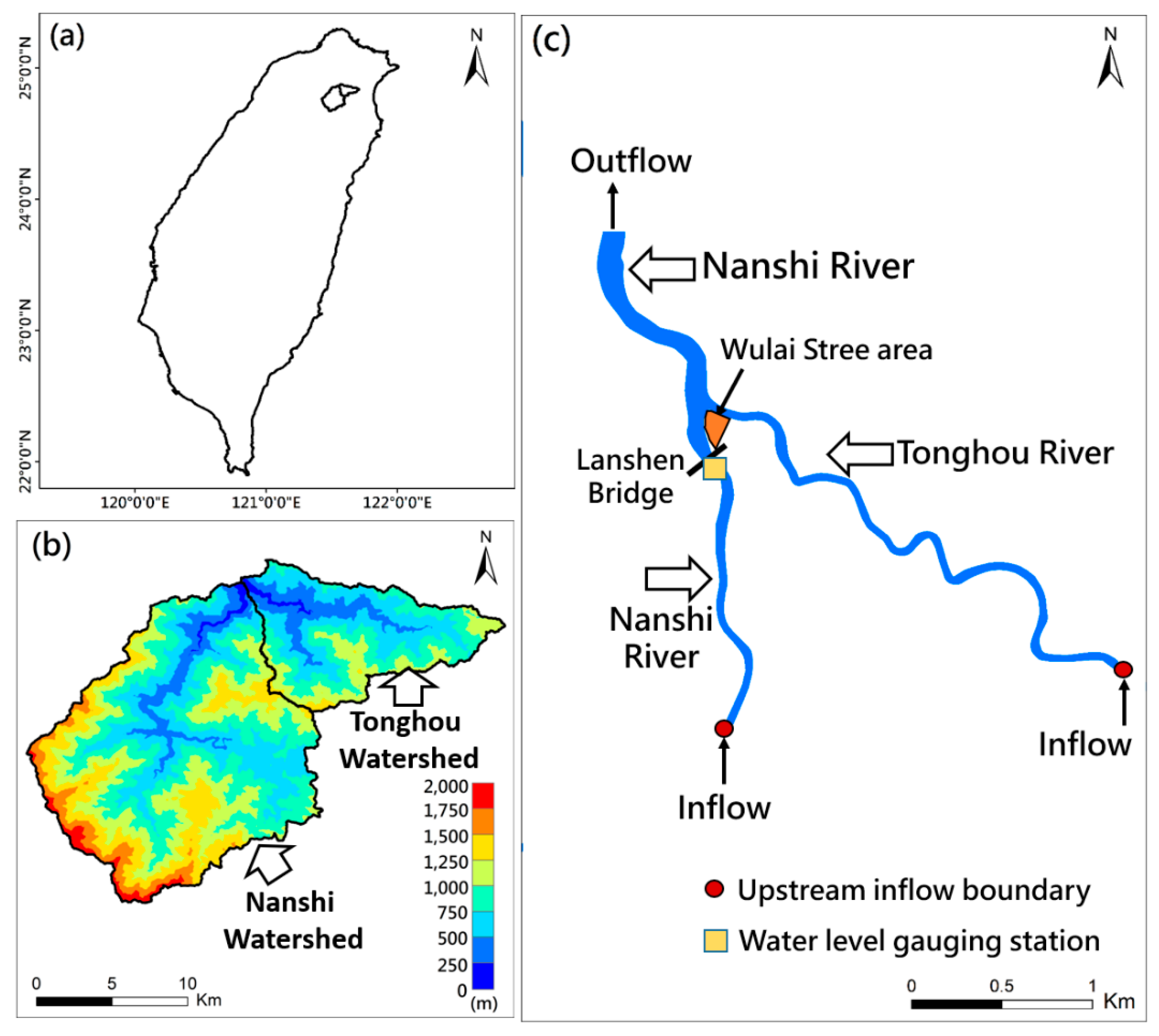
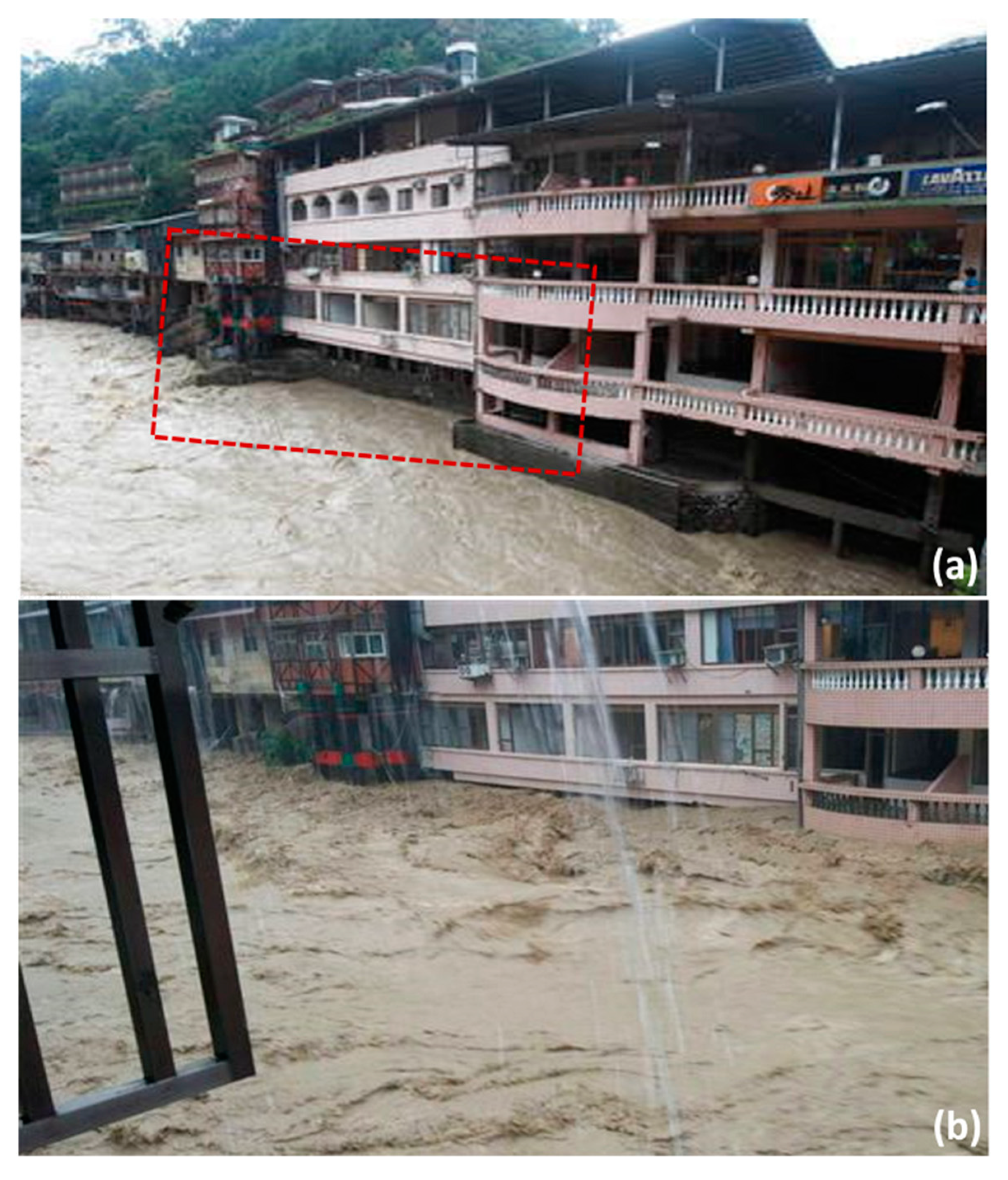
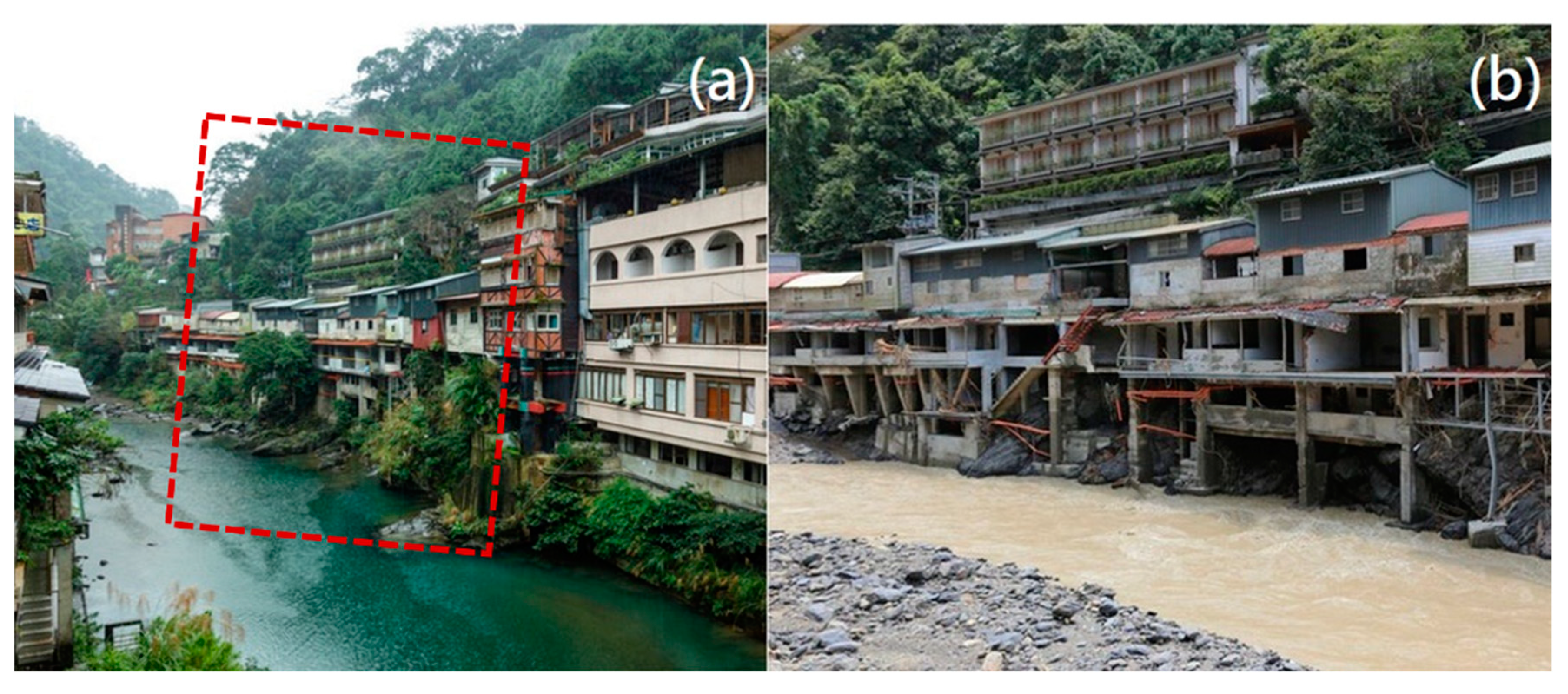
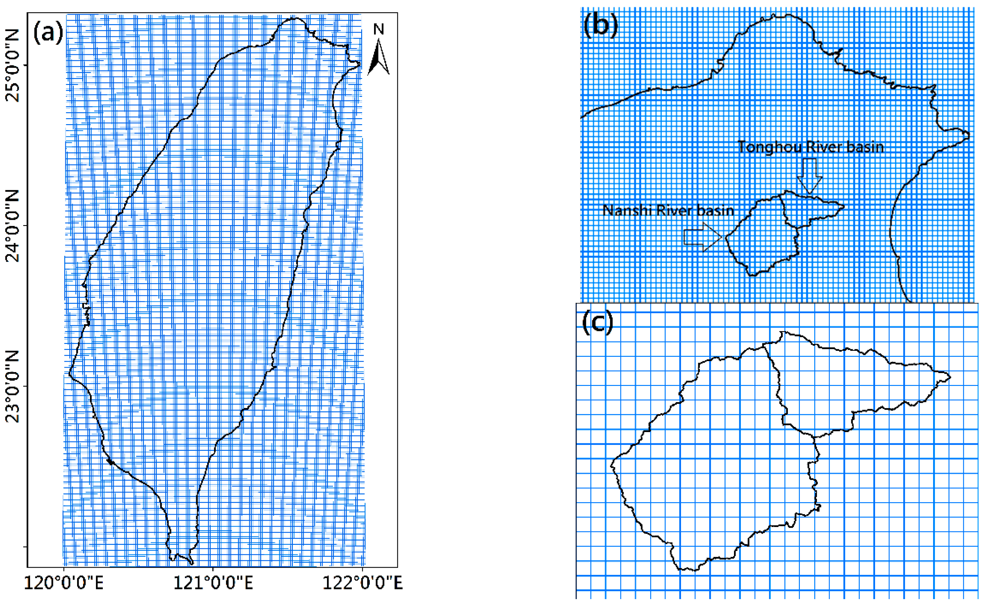
Mountainous areas account for approximately 70% of the total area in Taiwan; thus, mountainous river floodplains are prone to flash floods. The Wulai Street area is a famous scenic spot in the mountainous region of northern Taiwan (Figure 1a,b) and is located between the Nanshi and Tonghou watersheds (i.e., near the junction of the Nanshi and Tonghou Rivers) (Figure 1b,c). The small Nanshi and Tonghou watersheds only cover areas of 227 and 88 km², respectively, and have elevations ranging between 100 and 2000 m (Figure 1b). Flash flood events are expected to occur in such mountainous geographies. The Wulai Street area experienced severe flash floods induced by Typhoon Soudelor in August 2015. Torrents of water rushed down the mountain and submerged the buildings along the Tonghou River, and the flooding height was more than one floor (compare Figure 2a with Figure 2b) during Typhoon Soudelor (2015). The building exteriors were completely destroyed by the flash flood (compare Figure 3a with Figure 3b). Consequently, the development of an OFS is necessary for early warning, mitigation, and management of the disasters caused by flash floods in this mountainous area.

The aim of the present study was to develop an operational forecasting system for flash floods in mountainous areas in Taiwan by integrating numerical meteorological, hydrological, and hydrodynamic models and a visualization computer program. The details of the materials and methods are described in Section 2 and the results of the model validation and multi-model integration schemes are presented in Section 3. In Section 4, a discussion of the present study is given, which is followed by a summary and conclusions in Section 5.

2. Materials and Methods

2.1. Airborne Light Detection and Ranging (LiDAR) Data

A large amount of bathymetric and topographic data are the most fundamental requirement for river stage and flood simulation [17,18,19,20,21]; thus, airborne light detection and ranging (LiDAR) data have been increasingly applied in recent decades. Airborne LiDAR data can be employed for monitoring changes in landscape configurations, creating building structures, and constructing 3D models of urban areas. Airborne LiDAR has now become a popular tool for collecting accurate and dense topographic data due to its high resolution in both the horizontal and vertical directions and the efficiency (in terms of time and resources) of the measurement system. Airborne LiDAR data are typically blended with terrestrial surveys of riverbanks and riverbeds (e.g., measurements of riverine cross sections) to construct digital elevation models (DEMs) of river channels and floodplains. In this case, artificial terrestrial surveys are necessary because traditional lasers (red wavelength) cannot penetrate the water surface into the water body. However, on-site measurements are labor-intensive and dangerous, and surveyors cannot reach high mountains with rugged terrain. In the present study, a water-penetrating airborne LiDAR system (green wavelength) was adopted to measure the topographies in mountainous areas where rivers are prone to flash flooding; hence, extensive and accurate data on riverbeds, riverbanks, and river floodplains were readily acquired.

2.2. Atmospheric Model

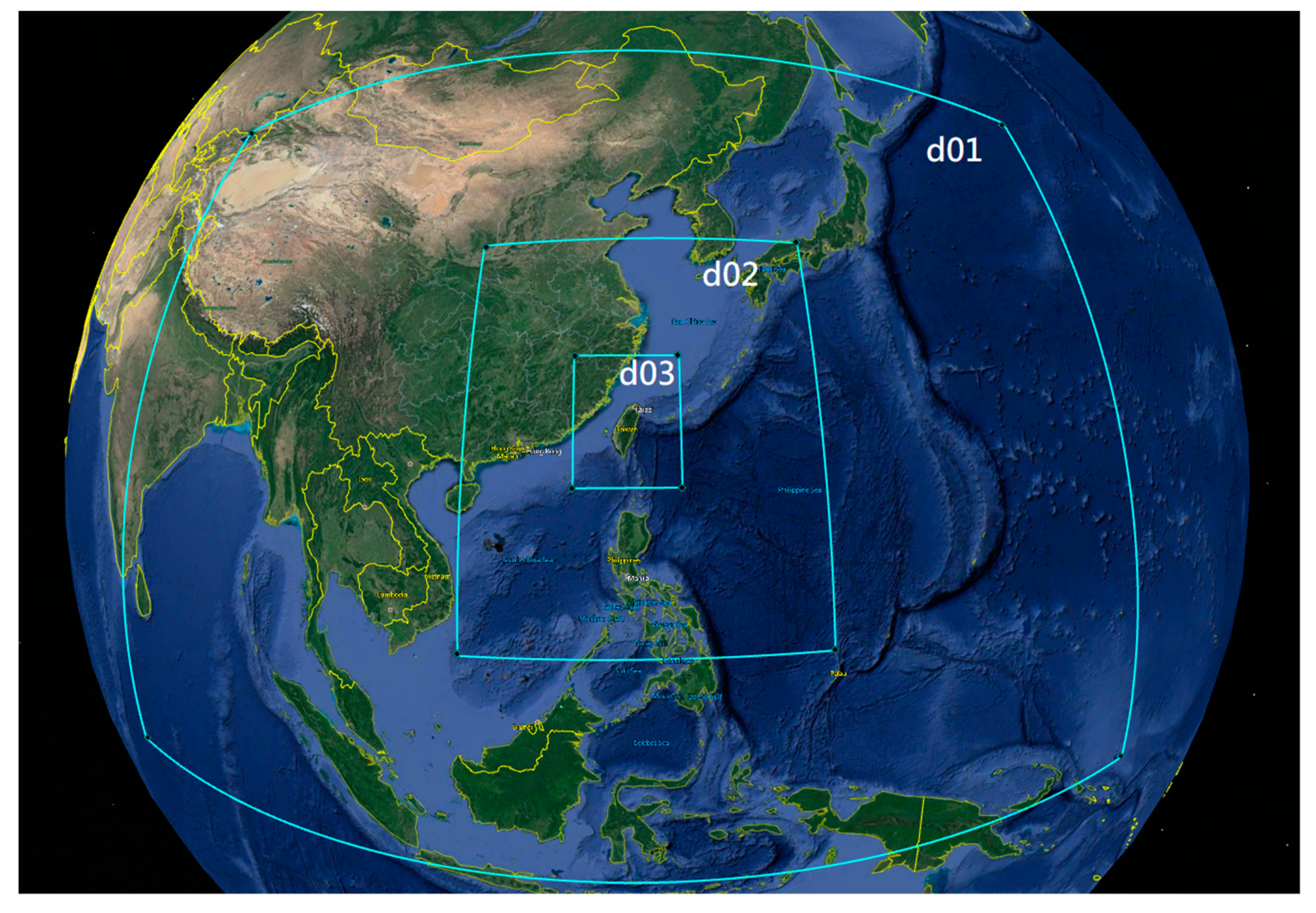
Reliable rainfall estimation is necessary to provide the meteorological conditions for the hydrological and hydrodynamic modeling of a watershed, especially for torrential rain. However, predicting extremely heavy rainfall in a short timescale is difficult and remains a challenge for numerical models; this is particularly true for mountainous terrain [22,23,24]. The weather research and forecasting (WRF) model [25] is an atmospheric model designed for both research and numerical weather prediction and is officially supported by the National Center for Atmospheric Research (NCAR). The WRF model has become the most widely used atmospheric model in the world and has been widely adopted for forecasting severe meteorological events such as heavy rainfall [26,27], typhoons or tropical cyclones [28,29], and thunderstorms [30,31]. Furthermore, WRF can focus on regional domains with resolutions beyond what most users can attain using global models [32]. The WRF model with three nested domains was employed to produce the rainfall forecast for the rainfall–runoff hydrological model in the present study because of the several advantages above-mentioned. Figure 4 shows the coverage of the three individual domains in the WRF model. The parent domain (d01) lies between −5.35°N–42.93°N and 77.91° E–159.99°E with a grid spacing of 45 km; the first nested domain (d02) covers 9.13°N–35.39°N and 109.65°E–134.41°E with a grid spacing of 15 km, and the second nested domain (d03) covers 20.02°N–28.29°N and 117.29°E–124.64°E with a grid spacing of 5 km.

The regional WRF model is currently an operational weather forecasting model at the National Science and Technology Center for Disaster Reduction (NCDR) of Taiwan. The predictions of the rainfall series from the WRF model at NCDR has been employed as inputs to estimate the runoff for several watersheds, then the estimated runoffs serve as inflows for predicting the water levels of the main rivers in Taiwan. The water level forecasts were in agreement with the measured data [33]. Hence, the rainfall data series from the WRF model at NCDR is believed to be reliable for the early warning of flash floods in mountainous areas in Taiwan.

2.3. Hydrological Model

Accurate predictions of runoff in a watershed are essential for flash flood mitigation and warning. The rainfall–runoff estimation techniques can be approximately classified as non-physically based and physically based models. For instance, artificial neural networks (ANNs) and support vector machines (SVMs) are well-known non-physically based models for streamflow and reservoir inflow forecasts [34,35,36,37]. Although the usage of ANNs and SVMs is quite simple, the key data-driven feature of these approaches makes them inadequate for forecasting runoff in mountainous areas with sparse observations. The hydrological characteristics of watersheds can be accounted for by using a physically based model. Additionally, only a small amount of measurement data are required for model validation. For example, Blazkova and Beven [38] used a simple semi-distributed model, namely TOPMODEL, to predict runoff and estimate flood frequency for a dam site in a large catchment in the Czech Republic. Therefore, a physically based rainfall–runoff hydrological model, the Clark unit hydrograph model (CUHM) [39], was utilized to generate the inflow time series (i.e., the upstream boundary conditions) for the Nanshi and Tonghou Rivers. The Clark unit hydrograph is essentially a synthetic unit hydrograph and is very effective in predicting rainfall runoff in a watershed with a complex shape and geomorphology and a large ratio of length to width [40,41]. Furthermore, the CUHM satisfies two evaluation conditions: (1) the hydrological model is able to forecast river flow operationally with at least 24 hours lead time every 6-hours per day; (2) the hydrological model is able to reproduce the hourly river discharges for the validation of the hydrodynamic model; and (3) the hydrological model is able to work on the Linux operating system. The input for the CUHM is precipitation data averaged over a watershed.

2.4. Hydrodynamic Model

One-dimensional and quasi-two-dimensional hydrodynamic models are widely used for flood inundation mapping [42]. Therefore, a derivative product, the SCHISM (semi-implicit cross-scale hydroscience integrated system model developed by Zhang et al. [43]), built from the original SELFE (semi-implicit Eulerian-Lagrangian finite element model developed by Zhang and Baptisa [44]), was employed to simulate and predict the river stages and water levels for the river channels and floodplains of the Nanshi and Tonghou watersheds. The SCHISM is a new cross-scale unstructured-grid model with many enhancements and upgrades such as a new implicit transport solver, a new horizontal viscosity formulation for generic unstructured grids, a new higher-order scheme for momentum advection, and the addition of quad elements [43]. The SCHISM and SELFE have been successfully applied to simulate the water levels (river stages) for a meandering river in southwestern Taiwan [45], to predict the inundation extent for a coastal and estuarine area due to storm surge and sea-level rise [46,47] in the southwestern and southern coasts of Taiwan, and the Superstorm Sandy-induced inundation in New York City [48] as well as to assess the potential for tidal power generation in the coastal waters of a small island [49]. The SCHISM-3D (a three-dimensional version of the SCHISM) with the barotropic mode (the water density gradient is ignored) was implemented in the present study; moreover, the SCHISM-2D (a two-dimensional version of the SCHISM) was used for comparison with the SCHISM-3D to evaluate model performance and efficiency.

The standard Navier–Stokes equations with hydrostatic and Boussinesq approximations in the Cartesian coordinate system are given as follows:

$$\frac{\partial u}{\partial z}+\frac{\partial v}{\partial z}+\frac{\partial w}{\partial z}=0$$

(1)

$$\frac{\partial \eta }{\partial t}+\frac{\partial }{\partial x}{\displaystyle {\int }_{-h}^{\eta }udz+}\frac{\partial }{\partial y}{\displaystyle {\int }_{-h}^{\eta }vdz=0}$$

(2)

$$\frac{Du}{Dt}=-g\frac{\partial \eta }{\partial x}+\frac{\partial }{\partial z}\left(\nu \frac{\partial u}{\partial z}\right)$$

(3)

$$\frac{Dv}{Dt}=-g\frac{\partial \eta }{\partial y}+\frac{\partial }{\partial z}\left(\nu \frac{\partial v}{\partial z}\right)$$

(4)

where $u(x,y,z,t)$ and $v(x,y,z,t)$ are the horizontal velocities in the x and y directions, respectively; $w(x,y,z,t)$ is the vertical velocity; $t$ is the time; $\eta (x,y,t)$ is the free-surface elevation; $h(x,y)$ is the bathymetric depth; g is the acceleration due to gravity; and $\nu$ is the vertical eddy viscosity.

The no-slip condition at the river bottom is replaced by a balance between the bottom frictional stress and the internal Reynolds stress as follows:

$$\nu \frac{\partial u}{\partial z}={\tau }_{bx},\mathrm{at}z=-h$$

(5)

$$\nu \frac{\partial v}{\partial z}={\tau }_{by},\mathrm{at}z=-h$$

(6)

The bottom stresses, ${\tau }_{bx}$ and ${\tau }_{by}$, are described using a quadratic drag law as follows:

$${\tau }_{bx}=\rho C_b\sqrt{u^2+v^2}u$$

(7)

$${\tau }_{by}=\rho C_b\sqrt{u^2+v^2}v$$

(8)

where $\rho$ is the density of water and $C_b$ is the bottom drag coefficient. $C_b$ can be parameterized as follows:

$$C_b=g{n}^2/H^{1/3}$$

(9)

where $n$ is the Manning coefficient and $H=\eta +h$.

As the Reynolds stress is constant inside the boundary layer, Equations (7) and (8) are applied at the top of the bottom cell as follows:

$$\nu \frac{\partial u}{\partial z}={\tau }_b,\mathrm{at}z=-h+{\delta }_b$$

(10)

$$\nu \frac{\partial v}{\partial z}={\tau }_b,\mathrm{at}z=-h+{\delta }_b$$

(11)

where ${\delta }_b$ is the thickness of the bottom computational cell.

In the SCHISM-2D, all three-dimensional variables of the SCHISM-3D (Equations (1)–(4)) become depth averaged. The SCHISM-2D assumes that the velocity is uniform in the vertical direction with one layer with the Manning formulation for the bottom drag (Equation (9)), therefore, a simple relation between the horizontal velocity and the free-surface elevation can be utilized to represent the momentum equations for the 2D model [50]. The governing equations in the two-dimensional form are as follows:

$$\frac{\partial \eta }{\partial t}+\frac{\partial uH}{\partial x}+\frac{\partial vH}{\partial y}=0$$

(12)

$$\frac{Du}{Dt}=-g\frac{\partial \eta }{\partial x}-\frac{{\tau }_{bx}}{\rho H}$$

(13)

$$\frac{Dv}{Dt}=-g\frac{\partial \eta }{\partial y}-\frac{{\tau }_{by}}{\rho H}$$

(14)

It should be noted that the bottom shear stresses in the SCHISM-3D are different from those in the SCHISM-2D because they depend on the depth-averaged velocity in the 2D model, but the bottom velocity in the 3D model.

2.5. Configuration of the SCHISM (Semi-implicit Cross-scale Hydroscience Integrated System Model) Model

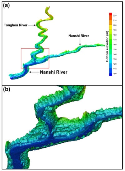
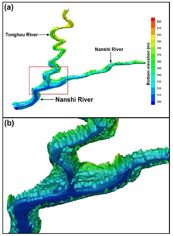
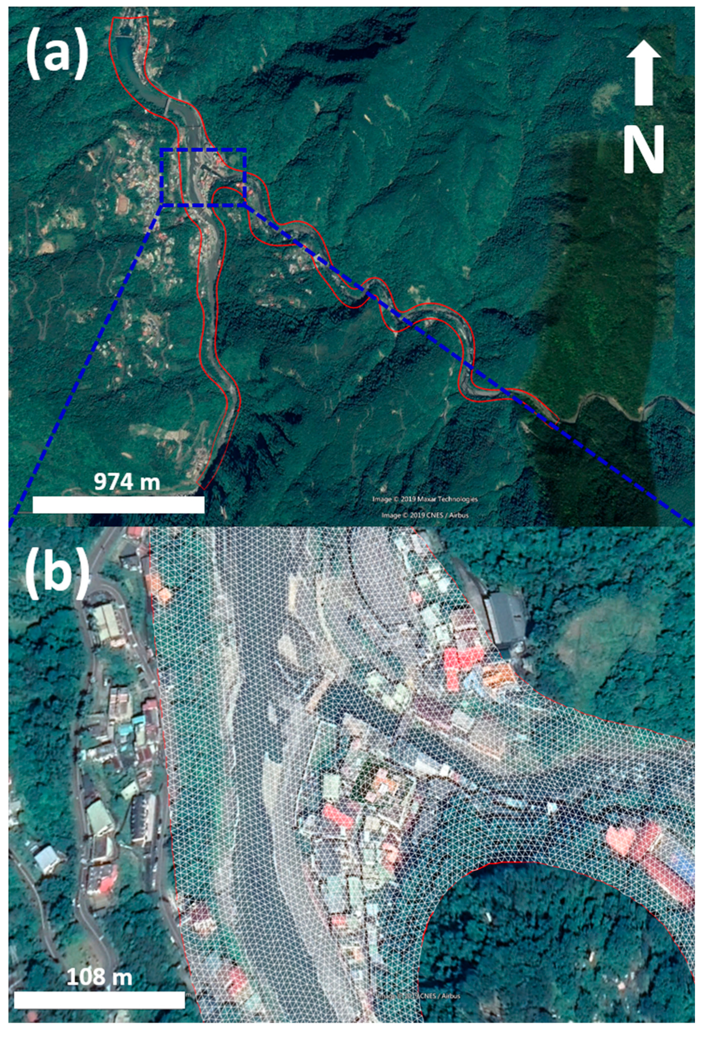
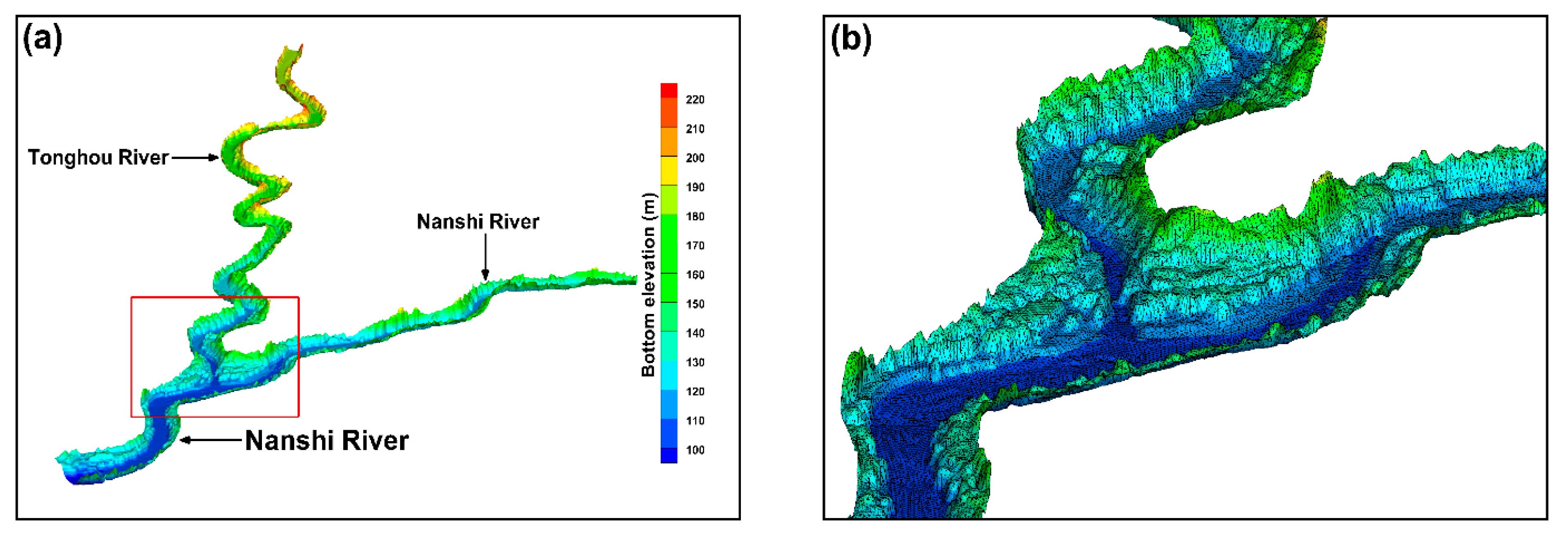
A computational domain including the main channel and floodplain of the Nanshi and Tonghou Rivers was developed for the SCHISM (inside of the red line shown in Figure 5a). This coverage is sufficiently wide for simulating riverine flash floods triggered by extreme rainfall events in mountainous areas. The SCHISM simulation domain consisted of 67,738 triangular elements and 35,144 nodes. Coarse meshes with 10-m resolutions were distributed in the upstream and downstream open boundaries beyond the flooding region, and fine meshes with 5-m resolutions were arranged along the river channels and flood-prone areas (i.e., the Wulai Street area) (Figure 5b). Although the simulation accuracy may be slightly improved using a higher-resolution mesh, the computing demand such as computer resources and execution time would be increased. The mesh resolution determined in the present study was thought to be sufficiently fine to represent the hydrodynamics of the river and floodplain. The gridded DEM data with a 1-m resolution for the SCHISM were constructed from airborne LiDAR as mentioned in Section 2.1. The gridded DEM data were interpolated to each node to represent the bottom elevations of the river channels and floodplain in the SCHISM after the unstructured grids were created. Figure 6 demonstrates a three-dimensional view of the topographies in the SCHISM (Figure 6a) and an enlargement of the junction of the Nanshi and Tonghou Rivers with high-resolution triangular meshes (Figure 6b). The great detail of the terrains can be further enhanced if high-resolution airborne LiDAR DEM data are utilized in the hydrodynamic model. The computational domain was divided into six layers in the vertical direction for the SCHISM-3D, but only into two layers for the SCHISM-2D. Two inflow boundaries were located in the upstream portions of the Nanshi and Tonghou Rivers, while an outflow boundary was assigned to the downstream portion of the Nanshi River (as shown in Figure 1c). Based on the type of river bottom material and numerical stability, a Manning coefficient (n in Equation (9)) of 0.025 and a time step of 2 s were set in the hydrodynamic model following model validation of the water levels for the Lansheng Bridge on the Nanshi River.

2.6. Gridded Rainfall Data

The Central Weather Bureau (CWB) and the Water Resource Agency (WRA) of Taiwan and the National Oceanic and Atmospheric Administration (NOAA)/National Severe Storms Laboratory (NSSL) of the United States have been involved in research and development to improve the monitoring and prediction of flash floods, debris flows, and severe storms in Taiwan. A system of quantitative precipitation estimation and segregation using multiple sensors (QPESUMS) was developed through this international collaboration. The QPESUMS system includes quantitative precipitation estimation (QPE, [51]) and quantitative precipitation forecast (QPF) products and provides high spatial (1.25 km by 1.25 km) and temporal (10-minute) resolution, gridded rainfall data by integrating the observations from weather radars, rain gauges, satellites, and numerical weather prediction model analyses. Figure 7 illustrates the distribution of the rainfall data grids from the QPESUMS for all of Taiwan (Figure 7a), northern Taiwan (Figure 7b), and the Nanshi and Tonghou watersheds (Figure 7c).

3. Results

3.1. Model Validation

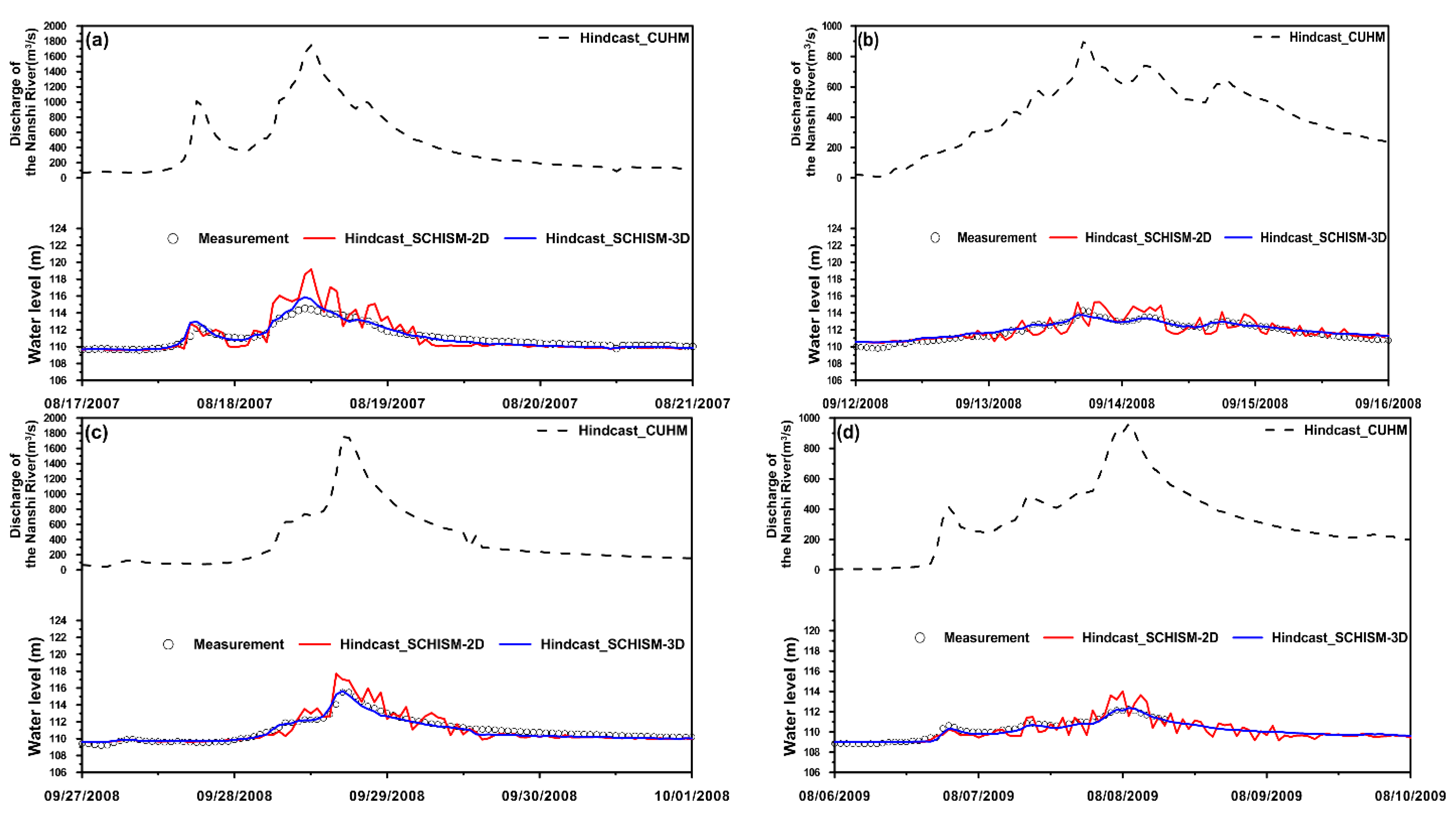
The model validation was conducted by comparing the hindcasted and measured water levels only for the Lansheng Bridge on the Nanshi River because rain gauging and discharge gauging stations are lacking in this region. The grids within or partially overlapping the Nanshi and Tonghou watersheds of the QPESUMS (as mentioned in Section 2.6 and shown in Figure 7c) serve as rainfall data inputs for the rainfall–runoff model (the CUHM as mentioned in Section 2.3) to calculate the upstream river discharge of the Nanshi and Tonghou Rivers. Four events with high water level variations at the Lansheng Bridge in 2007, 2008, and 2009 were hindcasted. The water level measurements at the Lansheng Bridge were provided by the WRA of Taiwan. The comparison of the modeled and observed water level time series and the inflow estimated by the CUHM are shown in Figure 8 (Figure 8a represents August 17–20, 2007; Figure 8b represents September 12–15, 2008; Figure 8c represents September 27–30, 2008; and Figure 8d represents August. 6–9, 2009). The highest water level measurement among these four events was approximately 116 m, with a discharge hindcast approaching 1800 m³s⁻¹, on September 28, 2008 (Figure 8c), while the lowest measurement was approximately 113 m, with a discharge hindcast approaching 900 m³s⁻¹, on August 8 and September 14, 2009 (Figure 8b,d). By adopting the SCHISM-3D, the hindcasting water level time series faithfully agree with the observations (blue lines in Figure 8). Although the same boundary conditions were imposed, the SCHISM-2D (red lines in Figure 8) produced unstable and wavelike water levels. This phenomenon was particularly significant at higher water levels.

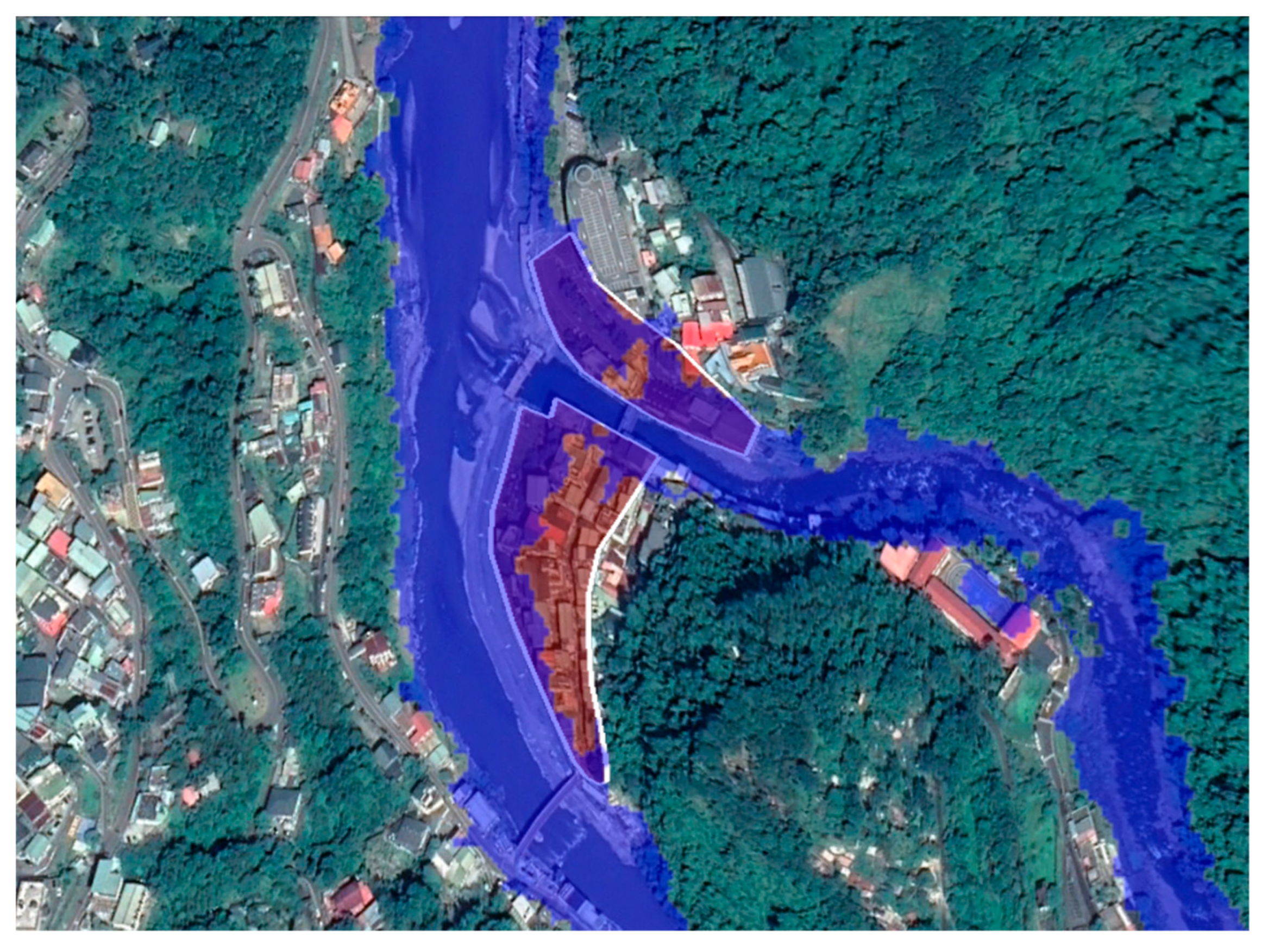
The Wulai Street area (as shown in Figure 5b) was once swamped by a Typhoon Soudelor-induced mountain flash flood in 2015. At that time, the water level gauge deployed at the Lansheng Bridge was washed away by the high flow in the Nanshi River. However, the WRA of Taiwan surveyed the flood areas in the regions along the Nanshi and Tonghou Rivers. The gridded rainfall data from August 7–12, 2015 were extracted for the CUHM to generate the discharge time series. Figure 9 demonstrates the hindcasted maximum water level distribution in the computational domain (Figure 9a) and the water level time series at the Lansheng Bridge (Figure 9b). The hindcasted water level rose rapidly within several hours. The highest water level exceeded the levee height (121.5 m) and reached 125 m at the Lansheng Bridge. The surveyed and hindcasted flood extents at the junction of the Nanshi and Tonghou Rivers are compared in Figure 10. Almost all of the Wulai Street area and the floodplains near the junction were flooded according to the site surveys (the areas inside the white line in Figure 10). The hindcasted flood extents were underestimated far from the riversides because the effects of rainfall on the flooding were excluded in the hydrodynamic model.

3.2. Implementation of an Operational Forecasting System (OFS) for Flash Floods in Mountainous Areas

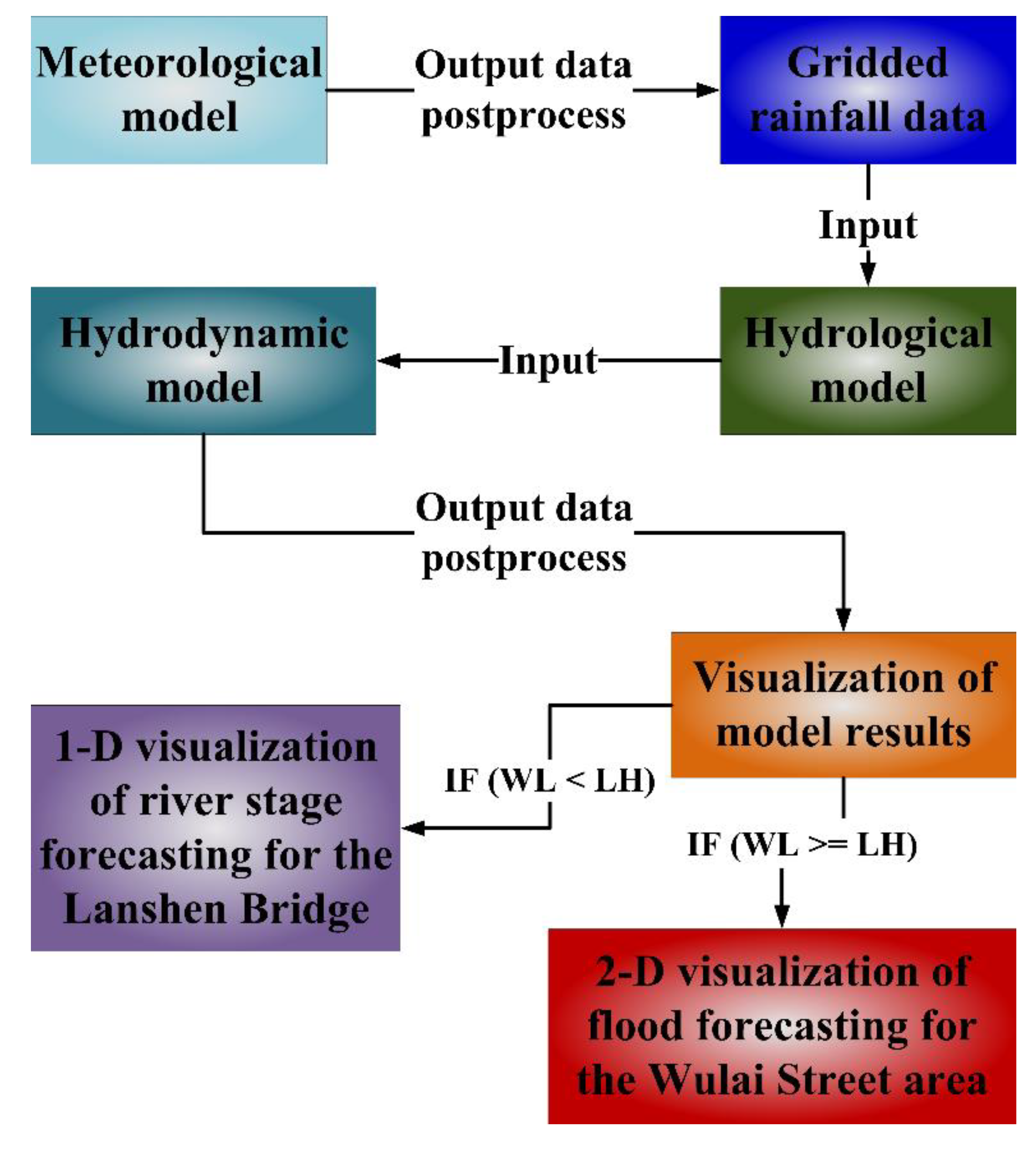
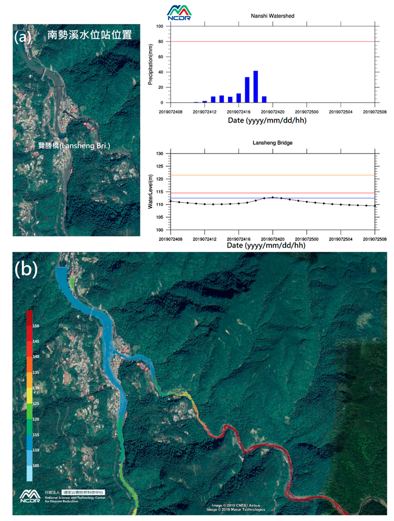
The weather forecast model (WRF), the rainfall–runoff hydrological model (CUHM), and the hydrodynamic model (SCHISM) were integrated to construct an OFS for mountain flash floods in the Wulai Street area. Rainfall forecasts produced by the WRF model are a primary element of the OFS. The original 5-km spatial resolution rainfall data in the second nested domain (d03) of the WRF model are interpolated on the square meshes with a spatial resolution of 1.25 km. In order to compare the rainfall predictions with observations, the coverage and spatial resolution were identical to the QPESUMS (as shown in Figure 7a) through the interpolation. The spatially averaged rainfall time series derived from the rainfall grids within or partially overlapping the Nanshi and Tonghou watersheds were applied to create the discharges for the SCHISM-3D. Finally, the water level time series for the Nanshi and Tonghou Rivers and for the riverine floodplains can be forecasted by the SCHISM-3D. Figure 11 elucidates a framework and flowchart of the OFS for flash floods in mountainous areas developed in the present study. The NCAR Command Language (NCL, as described in Appendix A) accounts for the visualization of water level forecasts in the OFS. This integrated scheme is fully automated through shell scripts on the Linux operating system. The OFS predicts water level variations over the next 24 hours. In this system, 1D visualization is carried out when the predicted water level is lower than the levee height at the Lansheng Bridge, whereas 2D visualization is performed if the predicted water level is higher than the levee height at the Lansheng Bridge. The 1D visualization of the OFS is shown in Figure 12a. The levee height (yellow line), alert level 1 (dark red line), and alert level 2 (blue line) were plotted with the forecasted water level time series for early warning. A snapshot of the 2D visualization for the OFS was superimposed on Google Earth and is shown in Figure 12b. The colored areas in Figure 12b indicate the hourly spatial distribution of the OFS predicted water levels. The entire process of the OFS for predicting the water levels in the next 24 hours can be completed within 45 minutes.

4. Discussion

The water level hindcasts appear unstable and wavelike using the SCHISM-2D, but appear smooth when employing the SCHISM-3D (as shown in Figure 8a–d). From the physical point of view, some inherent differences exist between the 2D and 3D models. For the 2D model, the bottom shear stress directly translates into mitigating the depth-averaged velocity and consequently increases the river stage [52]. In the 2D model, the horizontal velocity is depth-averaged (uniform in the vertical direction) and vertical shear is absent [50]. However, the bottom shear stress balances the vertical shear and only directly affects the horizontal velocity near the bottom cell in the 3D model. Additionally, a restriction to make a positive-define matrix is imposed on the numerical formula to solve free-surface elevation issues in the SCHISM-3D and consequently enhances the numerical stability for large friction in the shallow area (more detail can be found in [42]). This approach avoids unstable free-surface elevations occurring in the SCHISM-3D even if high flow conditions are present. A similar finding was also obtained in [45]. The 3D model undoubtedly has better performance in simulating the water level than the 2D model, although the 3D model is more computationally time-consuming than the 2D model. For example, on a high-performance computer with 64 cores, a single 24-hour requires 10.8 minutes of computing time using the SCHISM-3D but only 4 minutes is needed for the SCHISM-2D.

A small mountainous river usually experiences severe scouring, erosion, and/or sediment deposition during or after a torrential rainfall event (e.g., a typhoon) because a large volume of bedload is carried down the mountainsides to the river [53]. To ensure the accuracy of water level forecasts, a topographic survey of the study area utilizing airborne LiDAR should be conducted after the occurrence of an extreme rainfall event.

The ensemble forecast provides a more reliable rainfall forecast than a single deterministic prediction [54]. Thus, the ensemble rainfall prediction system could provide useful probability information and minimize uncertainty for runoff and water level forecasting and could be considered in the OFS in the future. Inclusion of the rainfall effect on the flooding simulation would improve the OFS for flash floods in mountainous areas. Moreover, further investigation on selecting the most appropriate model scheme for representing the real processes and detecting the dominant runoff generation mechanisms are expected to be improvements in flood prediction [55].

A triply nested WRF model with the highest resolution of 5-km implemented in the present study was a compromise between limited computer resources and execution time of the OFS (enough lead time for effective response is prioritized), even though it is sufficient to provide rainfall data for the OFS. The horizontal grid spacing less than ~5 km in a numerical weather prediction model (e.g., the WRF model) allows the explicit resolution of the dynamic and thermodynamic processes related to key terrain features that would significantly impact precipitation [56]. Therefore, a WRF model with a higher resolution (e.g., 3-km or 4-km) domain 3 (d03) should be constructed for predicting a flash-flood heavy rainfall event if more computing resources were acquired.

Dimitriadis et al. [40] investigated the uncertainty induced in several aspects of hydraulic modeling by applying the three models (HEC-RAS, LISFLOOD-FP, and FLO-2d) on a benchmark test with a mixed rectangular–triangular channel cross section. They found that the uncertainty in flood propagation mainly originates from the channel and floodplain friction as well as the inflow discharge. Owing to a lack of land cover/land use data, a Manning coefficient of 0.025 was set in the SCHISM-3D through the model validation of the water levels in the present study. To minimize the uncertainty caused by hydrodynamic/hydraulic modeling, the land cover/land use of the Nanshi and Tonghou watersheds should be surveyed in the future.

The OFS developed in the present study started being used at the National Science and Technology Center for Disaster Reduction (NCDR) in August 2019. To date, no extreme rainfall or typhoon events have occurred in the Wulai mountainous area; therefore, the water level predictions from the OFS have yet to be verified. However, the OFS will be continuously monitored and will be compared with the observed water level if any extreme rainfall or typhoon event occurs in the mountainous Wulai area. From an economical point of view, the possible application of the OFS to cover the whole mountainous area in Taiwan would be further evaluated as long as more gridded DEM data and high-performance computers were provided.

5. Summary and Conclusions

This study presents a multi-model integrated simulation scheme to construct an operational forecasting system (OFS) for flash flood emergency preparedness in two small mountainous watersheds in Taiwan. The OFS is composed of three numerical models and a visualization program. In the framework of the OFS, the gridded rainfall data in the watersheds are first forecasted by the Weather Research and Forecasting (WRF) model. The Clark unit hydrograph model (CUHM) acquires the gridded rainfall data from the WRF model and generates the river discharge time series as the upstream boundary conditions for the semi-implicit cross-scale hydroscience integrated system model (SCHISM). Then, the water levels and possible flood extents in the computational domain are predicted by the SCHISM. Finally, the NCAR Command Language (NCL) can efficiently generate a high-quality model image, thereby providing a visualization of the OFS results. This simulation scheme is appropriate for both forecasting and hindcasting, depending on the rainfall data being forecasted or hindcasted. The hindcasting water level time series of the Lansheng Bridge and the Typhoon Soudelor (2015)-induced flood extents were compared with the available measurements and surveys. In general, the results were comparable to the observed data, except for the underestimation of the flood extent due to the effect of rainfall on the flood, which is currently not included in the OFS. The gridded rainfall data from the WRF model were obtainable every six hours; hence, the OFS should be launched at the same time interval to secure reliable and feasible predictions. All components of the OFS are open-source software and available on the website. The OFS for the flash flood in the mountainous Nanshi and Tonghou watersheds is currently being used as an operational warning system at the National Science and Technology Center for Disaster Reduction (NCDR) of Taiwan. The forecasts can be browsed through the website of the NCDR WATCH (Weather Analysis and Taiwan Climate Hybrid monitor system, [57]). More operational forecasting systems for water-related hazards induced by severe weather conditions will continue to be developed in the near future.

References

- Borga, M.; Gaume, E.; Creutin, J.D.; Marchi, L. Surveying flash flood response: Gauging the ungauged extremes. Hydrol. Process. 2008, 22, 3883–3885. [Google Scholar] [CrossRef]
- Borga, M.; Stoffel, M.; Marchi, L.; Marra, F.; Jakob, M. Hydrogeomorphic response to extreme rainfall in headwater systems: Flash floods and debris flows. J. Hydrol. 2014, 518, 194–205. [Google Scholar] [CrossRef]
- Acosta-Coll, M.; Ballester-Merelo, F.; Martinez-Peiró, F.; De la Hoz-Franco, E. Real-Time Early Warning System Design for Pluvial Flash Floods—A Review. Sensor 2018, 18, 2255. [Google Scholar] [CrossRef] [PubMed]
- Matsuda, J.; Yamakoshi, T.; Tamura, K. Studies on alleviation of death accidents by flash floods. J. Hydrosci. Hydraul. Eng. 2010, 53, 487–492. [Google Scholar]
- Ruiz-Villanueva, V.; Díez-Herrero, A.; Stoffel, M.; Bollschweiler, M.; Bodoque, J.M.; Ballesteros, J.A. Dendrogeomorphic analysis of flash floods in a small ungauged mountain catchment (Central Spain). Geomorphology 2010, 118, 383–392. [Google Scholar] [CrossRef]
- Youssef, A.M.; Pradhan, B.; Hassan, A.M. Flash flood risk estimation along the St. Katherine road, southern Sinai, Egypt using GIS based morphometry and satellite imagery. Environ. Earth Sci. 2011, 62, 611–623. [Google Scholar] [CrossRef]
- Carpenter, T.M.; Sperfslage, J.A.; Georgakakos, K.P.; Sweeney, T.; Fread, D.L. National threshold runoff estimation utilizing GIS in support of operational flash flood warning systems. J. Hydrol. 1999, 224, 21–41. [Google Scholar] [CrossRef]
- Georgakakos, K.P. Real-Time Flash Flood Prediction. J. Geophys. Res. 1987, 92, 9615–9629. [Google Scholar] [CrossRef]
- Akbar, M.; Aliabadi, S.; Patel, R.; Watts, M. A fully automated and integrated multi-scale forecasting scheme for emergency preparedness. Environ. Model. Softw. 2013, 39, 24–38. [Google Scholar] [CrossRef]
- Georgakakos, K.P.; Graham, N.E.; Modrick, T.M.; Murphy, M.J., Jr.; Shamir, E.; Spencer, C.R.; Sperfslage, J.A. Evaluation of real-time hydrometeorological ensemble prediction on hydrologic scales in Northern California. J. Hydrol. 2014, 519, 2978–3000. [Google Scholar] [CrossRef]
- Modrick, M.T.; Georgakakos, K.P. The character and causes of flash flood occurrence changes in mountainous small basins of Southern California under projected climatic change. J. Hydrol. Reg. Stud. 2015, 3, 312–336. [Google Scholar] [CrossRef] [Green Version]
- Leandro, J.; Martins, R. A methodology for linking 2D overland flow models with the sewer network model SWMM 5.1 based on dynamic link libraries. Water Sci. Technol. 2016, 73, 3017–3026. [Google Scholar] [CrossRef] [PubMed]
- Barthélémy, S.; Ricci, S.; Morel, T.; Goutal, N.; Le Pape, E.; Zaoui, F. On operational flood forecasting system involving 1D/2D coupled hydraulic model and data assimilation. J. Hydrol. 2016, 534, 478–492. [Google Scholar] [CrossRef]
- Shin, E.T.; Shin, J.; Rhee, D.S.; Kim, H.J.; Song, C.G. Integrated Inundation Modeling of Flooded Water in Coastal Cities. Appl. Sci. 2019, 9, 1313. [Google Scholar] [CrossRef]
- SET News Channel. Available online: https://www.setn.com/ (accessed on 15 September 2019).
- The News Lens. Available online: https://www.thenewslens.com/article/22437 (accessed on 15 September 2019).
- Horritt, M.S.; Bates, P.D. Effects of spatial resolution on a raster based model of flood flow. J. Hydrol. 2001, 253, 239–249. [Google Scholar] [CrossRef]
- Casas, A.; Benito, G.; Thorndycraft, V.; Rico, M. The topographic data source of digital terrain models as a key element in the accuracy of hydraulic flood modelling. Earth Surf. Process. Landf. 2006, 31, 444–456. [Google Scholar] [CrossRef]
- Horritt, M.S.; Bates, P.D.; Mattinson, M.J. Effects of mesh resolution and topographic representation in 2D finite volume models of shallow water fluvial flow. J. Hydrol. 2006, 329, 306–314. [Google Scholar] [CrossRef]
- Cook, A.; Merwade, V. Effect of topographic data, geometric configuration and modeling approach on flood inundation mapping. J. Hydrol. 2009, 377, 131–142. [Google Scholar] [CrossRef]
- Caviedes-Voullieme, D.; Morales-Hernandez, M.; Lopez-Marijuan, I.; García-Navarro, P. Reconstruction of 2D river beds by appropriate interpolation of 1D cross-sectional information for flood simulation. Environ. Model. Softw. 2014, 61, 206–228. [Google Scholar] [CrossRef]
- Das, S.; Ashrit, R.; Iyengar, G.R.; Mohandas, S.; Gupta, M.D.; George, J.P.; Rajagopal, E.; Dutta, S.K. Skills of different mesoscale models over Indian region during monsoon season: Forecast errors. J. Earth Syst. Sci. 2008, 117, 603–620. [Google Scholar] [CrossRef] [Green Version]
- Li, L.; Gochis, D.J.; Sobolowski, S.; Mesquita, M.D. Evaluating the present annual water budget of a Himalayan headwater river basin using a high-resolution atmosphere-hydrology model. J. Geophys. Res. Atmos. 2017, 122, 4786–4807. [Google Scholar] [CrossRef]
- Chawla, I.; Osuri, K.K.; Mujumdar, P.P.; Niyogi, D. Assessment of the Weather Research and Forecasting (WRF) model for simulation of extreme rainfall events in the upper Ganga Basin. Hydrol. Earth Syst. Sci. 2018, 22, 1095–1117. [Google Scholar] [CrossRef] [Green Version]
- Skamarock, W.C.; Klemp, J.B.; Dudhia, J.; Gill, D.O.; Barker, D.M.; Duda, M.G.; Huang, X.Y.; Wang, W.; Powers, J.G. A Description of the Advanced Research WRF Version 3. NCAR Technical Note, NCAR/TN-475+STR; Mesoscale and Microscale Meteorology Division, National Center for Atmospheric Research: Boulder, CO, USA, 2008. [Google Scholar]
- Routray, A.; Mohanty, U.; Niyogi, D.; Rizvi, S.; Osuri, K.K. Simulation of heavy rainfall events over Indian monsoon region using WRF-3DVAR data assimilation system. Meteorol. Atmos. Phys. 2010, 106, 107–125. [Google Scholar] [CrossRef]
- Mohanty, U.; Routray, A.; Osuri, K.K.; Prasad, S.K. A study on simulation of heavy rainfall events over Indian region with ARW-3DVAR modeling system. Pure Appl. Geophys. 2012, 169, 381–399. [Google Scholar] [CrossRef]
- Routray, A.; Mohanty, U.; Osuri, K.K.; Kar, S.; Niyogi, D. Impact of satellite radiance data on simulations of Bay of Bengal tropical cyclones using the WRF-3DVAR modeling system. IEEE Trans. Geosci. Remote Sens. 2016, 54, 2285–2303. [Google Scholar] [CrossRef]
- Osuri, K.K.; Nadimpalli, R.; Mohanty, U.C.; Niyogi, D. Prediction of rapid intensification of tropical cyclone Phailin over the Bay of Bengal using the HWRF modelling system. Q. J. R. Meteorol. Soc. 2017, 143, 678–690. [Google Scholar] [CrossRef]
- Madala, S.; Satyanarayana, A.; Rao, T.N. Performance evaluation of PBL and cumulus parameterization schemes of WRF ARW model in simulating severe thunderstorm events over Gadanki MST radar facility–case study. Atmos. Res. 2014, 139, 1–17. [Google Scholar] [CrossRef]
- Osuri, K.; Nadimpalli, R.; Mohanty, U.; Chen, F.; Rajeevan, M.; Niyogi, D. Improved prediction of severe thunderstorms over the Indian Monsoon region using high-resolution soil moisture and temperature initialization. Sci. Rep. 2017, 7, 41377. [Google Scholar] [Green Version]
- Powers, J.G.; Klemp, J.B.; Skamarock, W.C.; Davis, C.A.; Dudhia, J.; Gill, D.O.; Coen, J.L.; Gochis, D.J. The Weather Research and Forecasting Model: Overview, system efforts, and future directions. Bull. Am. Meteorol. Soc. 2017, 98, 1717–1737. [Google Scholar] [CrossRef]
- Chen, W.B.; Jang, J.H.; Chang, C.H. Predicting River Stages Using an Operational Forecasting System; National Science and Technology Center for Disaster Reduction: New Taipei City, Taiwan, 2017. (In Chinese) [Google Scholar]
- Wu, M.C.; Lin, G.F.; Lin, H.Y. Improving the forecasts of extreme streamflow by support vector regression with the data extracted by self organizing map. Hydrol. Process. 2014, 28, 386–397. [Google Scholar] [CrossRef]
- Lin, G.F.; Chen, G.R.; Huang, P.Y. Effective typhoon characteristics and their effects on hourly reservoir inflow forecasting. Adv. Water Resour. 2010, 33, 887–898. [Google Scholar] [CrossRef]
- Lin, G.F.; Wu, M.C. An RBF network with a two-step learning algorithm for developing a reservoir inflow forecasting model. J. Hydrol. 2011, 405, 439–450. [Google Scholar] [CrossRef]
- Lin, G.F.; Chou, Y.C.; Wu, M.C. Typhoon flood forecasting using integrated two stage support vector machine approach. J. Hydrol. 2014, 486, 334–342. [Google Scholar] [CrossRef]
- Blazkova, S.; Beven, K. Flood frequency estimation by continuous simulation of subcatchment rainfalls and discharges with the aim of improving dam safety assessment in a large basin in the Czech Republic. J. Hydrol. 2004, 292, 153–172. [Google Scholar] [CrossRef]
- Clark, C.O. Storage and the unit hydrograph. Trans. Am. Soc. Civ. Eng. 1945, 110, 1419–1488. [Google Scholar]
- Sabol, G.V. Clark unit hydrograph and R-parameter estimation. J. Hydraul. Eng. ASCE 1988, 114, 103–111. [Google Scholar] [CrossRef]
- Ahmad, M.M.; Ghumman, A.R.; Ahmad, S. Estimation of Clark’s Instantaneous Unit Hydrograph Parameters and Development of Direct Surface Runoff Hydrograph. Water Resour. Manag. 2009, 23, 2417–2435. [Google Scholar] [CrossRef]
- Dimitriadis, P.; Tegos, A.; Oikonomou, A.; Pagana, V.; Koukouvinos, A.; Mamassis, N.; Koutsoyiannis, D.; Efstratiadis, A. Comparative evaluation of 1D and quasi-2D hydraulic models based on benchmark and real-world applications for uncertainty assessment in flood mapping. J. Hydrol. 2016, 534, 478–492. [Google Scholar] [CrossRef]
- Zhang, Y.; Ye, F.; Stanev, E.V.; Grashorn, S. Seamless cross-scale modeling with SCHISM. Ocean Model. 2016, 102, 64–81. [Google Scholar] [CrossRef] [Green Version]
- Zhang, Y.; Baptisa, A.M. SELFE: A semi-implicit Eulerian-Lagrangian finite-element model for cross-scale ocean circulation. Ocean Model. 2008, 21, 71–96. [Google Scholar] [CrossRef]
- Chen, W.B.; Liu, W.C. Modeling the Influence of River Cross-Section Data on a River Stage Using a Two-Dimensional/Three-Dimensional Hydrodynamic Model. Water 2017, 9, 203. [Google Scholar] [CrossRef]
- Chen, W.B.; Liu, W.C. Modeling Flood Inundation Induced by River Flow and Storm. Water 2014, 6, 3182–3199. [Google Scholar] [CrossRef]
- Chen, W.B.; Liu, W.C. Assessment of storm surge inundation and potential hazard maps for the southern coast of Taiwan. Nat. Hazards 2016, 82, 591–616. [Google Scholar] [CrossRef]
- Wang, H.V.; Loftis, J.D.; Liu, Z.; Forrest, D.; Zhang, J. The storm surge and sub-grid inundation modeling in New York City during hurricane Sandy. J. Mar. Sci. Eng. 2014, 2, 226–246. [Google Scholar] [CrossRef]
- Chen, W.B.; Chen, H.; Lin, L.Y.; Yu, Y.C. Tidal Current Power Resource and Influence of Sea-Level Rise in the Coastal Waters of Kinmen Island, Taiwan. Energies 2017, 10, 652. [Google Scholar] [CrossRef]
- Zhang, Y.J.; Witter, R.C.; Priest, G.R. Tsunami-tide interaction in 1964 Prince William Sound tsunami. Ocean. Model. 2011, 40, 246–259. [Google Scholar] [CrossRef]
- Zhang, J.; Howard, K.; Chang, P.L.; Chiu, P.T.K.; Chen, C.R.; Langston, C.; Xia, W.W.; Kaney, B.; Lin, P.F. High-Resolution QPE System for Taiwan, Data Assimilation for Atmospheric, Oceanic, and Hydrologic Applications; Park, S.K., Xu, L., Eds.; Springer: Berlin, Germany, 2009; pp. 147–162. [Google Scholar]
- Kim, T.B.; Choi, S. Depth-averaged modeling of vegetated open-channel flows using finite element method. In Proceedings of the 16th IAHR-APD Congress and 3rd Symposium of IAHR-ISHS, Chapter in Advances in Water Resources and Hydraulic Engineering; Springer: Berlin/Heidelberg, Germany, 2008; pp. 411–416. [Google Scholar]
- Matsuda, I. River Morphology and Channel Processes. In Fresh Surface Water; Dooge, J.C.I., Ed.; In Encyclopedia of Life Support Systems (EOLSS), Developed under the Auspices of the UNESCO; Eolss Publishers: Oxford, UK, 2004. [Google Scholar]
- Hsiao, L.T.; Yang, M.J.; Lee, C.S.; Kuo, H.C.; Shih, D.S.; Tsai, C.C.; Wang, C.J.; Chang, L.Y.; Chen, Y.C.; Feng, L.; et al. Ensemble forecasting of typhoon rainfall and floods over a mountainous watershed in Taiwan. J. Hydrol. 2013, 506, 55–68. [Google Scholar] [CrossRef] [Green Version]
- Iacobellis, V.; Fiorentino, M.; Gioia, A.; Manfreda, S. Best fit and selection of theoretical flood frequency distributions based on different runoff generation mechanisms. Water 2010, 2, 239–256. [Google Scholar] [CrossRef]
- Hong, S.Y.; Lee, J.W. Assessment of the WRF model in reproducing a flash flood heavy rainfall event over Korea. Atmos. Res. 2009, 93, 818–831. [Google Scholar] [CrossRef]
- Weather Analysis and Taiwan Climate Hybrid monitor system (WATCH). Available online: https://watch.ncdr.nat.gov.tw/watch_wlfst (accessed on 15 September 2019).
- Brown, J.R.; Earnshaw, R.; Jern, M.; Vince, J. Visualization: Using Computer Graphics to Explore Data and Present Information; John Wiley & Sons: New York, NY, USA, 1995. [Google Scholar]
Figure 1.
Locations of the study area: (a) country, (b) watersheds, and (c) rivers.
Figure 2.
The initial stage (a) and the later stage (b) of the mountain flash flood along the Tonghou River induced by Typhoon Soudelor (2015) (Photo source: [15]).
Figure 3.
The exteriors of buildings along the Tonghou River (a) before and (b) after the mountain flash flood induced by Typhoon Soudelor (2015) (Photo source: [16]).
Figure 4.
The extents in the WRF model for Domain 1 (d01) with a grid spacing of approximately 45 km, Domain 2 (d02) with a grid spacing of approximately 15 km, and Domain 3 (d03) with a grid spacing of approximately 5 km.
Figure 5.
The computational domain of the hydrodynamic model (a) and an enlargement of the Wulai Street area with the high-resolution unstructured grids of the hydrodynamic model (b).
Figure 6.
3D view of the bottom elevations of the hydrodynamic model (a) and an enlargement of the junction of the Nanshi and Tonghou Rivers with high-resolution triangular meshes (b).
Figure 7.
The 1.25 km by 1.25 km rainfall data grids (blue meshes) of quantitative precipitation estimation and segregation using multiple sensors (QPESUMS) and interpolated from the WRF model for (a) all of Taiwan, (b) an enlargement of northern Taiwan, and (c) an enlargement of the Nanshi and Tonghou watersheds.
Figure 8.
Comparison of the modeled and observed water levels at the Lansheng Bridge during the different high-flow events: (a) represents August 17–20, 2007; (b) represents September 12–15, 2008; (c) represents September 27–30, 2008; and (d) represents August 6–9, 2009. The upper panels in each figure are the inflow derived from the CUHM (Clark Unit Hydrograph Model).
Figure 9.
Hindcasting of the highest water level distribution (a) and river stage time series at the Lansheng Bridge (b) during Typhoon Soudelor (2015).
Figure 10.
Comparison of the hindcast (blue coverage) and survey (inside the white lines) for the Typhoon Soudelor (2015)-induced flood extent at the junction of the Nanshi and Tonghou Rivers.
Figure 11.
A framework of the operational forecasting system (OFS) for a mountain flash flood (WL and LH represent the water level and the levee height at the Lansheng Bridge, respectively).
Figure 12.
1D (a) and 2D (b) visualization of the operational forecasting system (OFS) for a mountain flash flood. In (a), the left panel is the mountain flash flood warning area and the location of the Lansheng Bridge, the upper-right panel represents the hourly rainfall averaged over the Nanshi watershed, and the lower-right panel shows the predicted water level time series of the Lansheng Bridge for the next 24 hours. The colored area in (b) indicates the spatial distribution of the predicted water levels.
© 2019 by the authors. Licensee MDPI, Basel, Switzerland. This article is an open access article distributed under the terms and conditions of the Creative Commons Attribution (CC BY) license (http://creativecommons.org/licenses/by/4.0/).
Share and Cite
MDPI and ACS Style
Chen, Y.-M.; Liu, C.-H.; Shih, H.-J.; Chang, C.-H.; Chen, W.-B.; Yu, Y.-C.; Su, W.-R.; Lin, L.-Y. An Operational Forecasting System for Flash Floods in Mountainous Areas in Taiwan. Water 2019, 11, 2100. https://doi.org/10.3390/w11102100
AMA Style
Chen Y-M, Liu C-H, Shih H-J, Chang C-H, Chen W-B, Yu Y-C, Su W-R, Lin L-Y. An Operational Forecasting System for Flash Floods in Mountainous Areas in Taiwan. Water. 2019; 11(10):2100. https://doi.org/10.3390/w11102100
Chicago/Turabian StyleChen, Yung-Ming, Che-Hsin Liu, Hung-Ju Shih, Chih-Hsin Chang, Wei-Bo Chen, Yi-Chiang Yu, Wen-Ray Su, and Lee-Yaw Lin. 2019. "An Operational Forecasting System for Flash Floods in Mountainous Areas in Taiwan" Water 11, no. 10: 2100. https://doi.org/10.3390/w11102100
Note that from the first issue of 2016, this journal uses article numbers instead of page numbers. See further details here.