Changes of Annual Precipitation and Probability Distributions for Different Climate Types of the World


1
Civil Engineering Department, Indian Institute of Technology, Roorkee 247667, India
2
Adjunct Faculty, Department of Civil and Environmental Engineering, University of Missouri, Columbia, MO 65211, USA
*
Author to whom correspondence should be addressed.
Water 2019, 11(10), 2092; https://doi.org/10.3390/w11102092
Submission received: 6 July 2019
/
Revised: 11 August 2019
/
Accepted: 16 August 2019
/
Published: 8 October 2019
(This article belongs to the Special Issue Urban Water Accounting)
Abstract
:Analysis of Spatio-temporal changes in precipitation (Pre) on the land surface of the earth was the focus of this study. Thiel-Sen median slopes and Modified Mann-Kendall (MMK) test were utilized to draw inferences. Majority of the regions were identified to show an increasing trend of annual precipitation except some of the low to mid-latitude regions in Northern hemisphere. The trends of wet-day frequency (Wet) were found in agreement with precipitation for most of the regions, but the inverse relationship was found for the subtropical regions of Northern hemisphere. These changes were examined for the world climate types based on Koppen-Gieger climate classes. Also, it was tried to find the probability distribution, which best describes the annual precipitation pattern in different climate types of the world among 21 commonly assumed probability distributions.
1. Introduction
Global warming is found to be responsible for the change in long term climate, which is termed as climate change. Many observed changes in climatic variables are found to be unprecedented before mid of 20th Century [1]. Climate change is found to be affecting the atmosphere, oceans, snow, and ice cover. Precipitation patterns across the globe have changed due to global warming [2,3]. Mishra et al. [4] reported the increase of heatwaves and a decrease in cold waves in the urban areas of the world. Warming of permafrost was also reported by Biskaborn et al. [5], which might further amplify global warming. Gudmundsson et al. [6] reported the significant changes in the mean and extreme values of streamflow across the globe.
Trend estimation is the primary exercise to understand the changes in climate. Trend estimation involves the computation of two characteristics of the time series, i.e., (i) trend direction and magnitude and (ii) significance of the trend. Sen slope estimate [7] has been widely used in climate studies to estimate the direction and magnitude as it is robust and insensitive to the outliers [8,9,10]. However, this method cannot be used to find the significance of the trends. So, Mann-Kendall (MK) test [11,12] is widely used for this purpose. The presence of serial correlation cannot be ruled out in the observed hydrometeorological data, but most of the researchers computed the significance of trend without considering the autocorrelation structure of the data [13,14,15,16,17]. Studies have found that the presence of positive serial correlation affects the ability of the MK test to correctly assess the significance of the trend [18]. The pre-whitening process has been used in different studies to remove the autocorrelation [19,20,21]. Bayazit et al. [22] argued that pre-whitening procedures are only useful when there is little to no trend. The pre-whitening results in the loss of some amount of existing trend [23]. MMK (Modified Mann-Kendall) test [24] is widely used to detect the significance of the trend in the presence of serial autocorrelation as this test considers the effect of serial correlation [25,26,27]. MMK and Sen Slope methods were adopted to find the significance of trends in this study.
The precipitation patterns are also not untouched by global warming. The world faced a high number of extreme weather conditions, including rare events of rainfall in the last decade [28]. The studies have found that the majority of lands may get stronger precipitation extremes than weaker [29]. Model simulations also suggest a net increase in global precipitation but the distribution may not be uniform [30]. Feng et al. [31] used high-resolution simulated data to study the global changes in the amount, intensity, and frequency of precipitation. They found an increase in precipitation except for latitude 15–40° N. The frequency of light and heavy precipitation was found to be increasing. Effect of climate change on precipitation has been studied largely on the regional scale than global scale [2,32,33]. Majority of these studies focused on finding the changes in climate extremes [25,34,35,36]. Raghvendra et al. [35] reported the increase in number and intensity of thunderstorm in the Congo Basin, Central Africa; however, the net rainfall was found to be decreased. Thomas and Nigam [37] reported the expansion of Sahara desert, South Africa, and warming trends of Southern regions than Northern regions. Choudhary et al. [36] detected a rapid decrease in monsoon rainfall in the wettest place on the earth, North-East India, in the last four decades. The changes in annual total precipitation directly affect the water budget of the regions and are crucial for maintaining adequate water resources. So, we limited our study to find the long-term changes in annual precipitation over the landmass of the earth.
Wet-day frequency is also an important parameter to assess the changes in precipitation patterns in the regions. It is defined by the number of rainy days at a particular location. This is a good parameter indicating the length of wet or dry spells. Change in the frequency of extreme events have been particularly reported in several studies [6,38,39]; however, the wet spells of moderate-intensity are equally crucial to maintain the water budget of the region. So, in this study, it was tried to find the relationship of changes in precipitation with a change in the number of wet days to estimate the patterns of extreme as well as moderate events and to check the probability of flooding or droughts in different parts of the world.
As global warming is not affecting every region of the world uniformly, in this study, it was tried to find the changes in precipitation patterns in different climate types of the world. Koppen-Geiger world map of climate type [40] is a widely adopted climate map to study different climate types [41,42,43]. The world climate is divided into five major climate types, i.e., Tropical, Arid, Temperate, Cold, and Polar, represented by A, B, C, D, and E letter, respectively, based on long monthly record (1901–2000) of temperature and precipitation. This classification is based on the combined effect of precipitation, temperature, seasonal variations, and extreme weather conditions. Kottek et al. [44] updated the Koppen climate type world map using gridded climate data from mid of 20th century. Peel et al. [45] used long term precipitation and temperature data set to update Koppen climate types. Beck et al. [46] also presented an updated climate type world map for the present day (1980–2016) and projected future (2071–2100). As it was required to identify the long term changes in different climate types of the world, the climate type map updated by Peel et al. [45] was considered in this study.
The trends show the behavior of the time series in the time domain, but global warming is not only affecting the precipitation patterns in the time domain but also in the frequency domain. In this study, it was tried to find the changes in the frequencies of the precipitation patterns in different locations using different probability distributions. The knowledge of correct probability distribution resembling the rainfall patterns is of the matter of eminent significance as the wrong estimation of design rainfall may lead to either lower/higher estimation, which in turn may cause the failure of hydraulic structures or an unnecessary increase in the cost. A good review of previous studies by Ye et al. [47] indicated that majority of the studies related to finding best-fit probability distribution were focused on daily time scale or extreme events [48,49,50]. The widely adopted probability distribution to represent the daily extreme rainfall patterns are Normal, Exponential, Log-Normal, Pearson, Log-Pearson (III), Weibull, Pareto, Generalized Gamma, Generalized Extreme Value (GEV), Logistic, Generalized Logistic, Wakebay, and Kappa. Only a few of the available studies are focused on finding global patterns of the best-fit probability distribution for precipitation. A review of available studies focusing on fitting probability distribution to daily extreme precipitations can be found in available literature [51,52,53]. It has been communicated that GEV III (Freshet distribution) can be best assumed to fit the daily extreme precipitation. However, it is known that the assumed best-fit probability distribution at different scale cannot be adopted to represent the frequency of precipitation at the annual scale. A study focused on finding a probability distribution function (PDF), which may represent global patterns of annual total precipitation, could not be found. The annual behavior of precipitation patterns is important to plan the water resources for the future. Extreme events do not generally affect the annual amount of rainfall, so even if the frequency of extreme events is found to be changing, the water availability for the year can be managed if the changes in annual precipitation are known. So, in this study, we tried to find the probability distribution, which can best define the annual precipitation across the globe. Here, 21 types of widely used probability distributions, which are assumed to be describing rainfall patterns by different researchers, were used in this study.
The objective of this study was to find the global-scale variations in annual precipitation (Pre) corresponding to changes in wet-day frequency (Wet) using high-resolution observed data. Changes in Pre with Wet might be useful to find the frequency of high or low precipitation events for a particular region. Changes in precipitation have not been analyzed for different climatic regions of the world earlier. We tried to find the relationship with increase/decrease in intensity of rainfall with the climate type of the region. Finally, the frequency distribution of annual precipitation patterns was also found out by fitting different PDFs.
2. Materials and Methods
2.1. Study Area and Data
This study covered the entire landmass of the world, excluding Antarctica. Global high resolution gridded (0.5° longitude and 0.5° latitude) Pre and Wet data for years 1901 to 2016 provided by Climatic research unit (CRU) of East Anglia [54] were used in this study.
CRU provides monthly total values for these variables, which are derived from station data provided by the World Meteorological Organization (WMO) in collaboration with the US National Oceanographic and Atmospheric Administration (NOAA). Pre is the primary variable of the CRU dataset and is solely based on observed station data [55]. The half-degree grid cells were defined where at least one station data was available within 450 km from the center of the grid. Less interpolation was required for precipitation because of higher station density. Wet is the second variable of CRU dataset and is derived from Pre using the empirical formula given by New et al. [56]. Wet varies from zero to maximum number days in a month, as it counts the number of wet days in a month even if the amount of precipitation is less. The CRU data have been widely used in different hydrological and climate change impact studies [57,58,59,60]. CRU data was earlier compared with similar global datasets, i.e., University of Delaware (UDEL) (data provided by the NOAA/OAR/ESRL PSD, Boulder, Colorado, USA, from their Web site at https://www.esrl.noaa.gov/psd/) and Global Precipitation Climatology Center (GPCC) [61] and were found consistent.
2.2. Data Preparation and Methodology
The analysis of annual precipitation patterns of 116 years (1901–2016) for more than 57,000 locations (grid points) across the globe has been done. Several quality checks have already been adopted during data preparation by CRU, assuring good quality of data. However, it was observed that some of the grid points (even though having monthly data) of the same annual series were repeated for several years. The grid points, having such erroneous data, were not considered in this study. Monthly total ‘Pre’ and ‘Wet’ were converted to annual totals and used for further analysis. As previously discussed, autocorrelation highly influences the trend component, so the presence of autocorrelation was checked in the data.
Autocorrelation may be defined as cross-correlation of the time series with itself at defined time lag. The time lag by ‘k’ times represents the correlation of the series with the series , where ‘N’ is the total number of data points in the time series. Autocorrelation (r) at lag k for the time series is given by
here, is the autocorrelation at lag k, is the covariance at lag k,
and are mean and variance, respectively.
Autocorrelation is said to be significant if it is out of the range of , where k is the value of standard normal variate at a defined significance level, and N is sample size [62]. A significance level of 5% is adopted to check the significance of autocorrelation in this study.
The trends were estimated using non-parametric Sen’s Slope estimate. It is the most popular nonparametric technique for the estimation of a linear trend as it is robust and insensitive to outliers [63]. The parameter is computed as:
where Xi and Xk are data at j and k times in time series .
The values of are arranged in ascending order, and median of the slopes or Sen’s slope (β) is computed as
The positive or negative sign of β indicates rising and falling trend, respectively, and its value defines the magnitude of the trend. However, the significance of the trend cannot be directly known by this method. So, the MK test [11,12] is generally used to estimate the significance of the trend. The significance of trend is calculated using standard normal test static ‘Zc’, which is compared with standard normal deviate ‘Zs’ at defined significance level ‘α’. The null hypothesis H0 of no trend is rejected if .
where S is the MK test static.
here, N is the size of the series, and are data at j and k times in time series . is the signum function which is 1, 0, −1 when , respectively.
The variance of S is calculated as
here, m is the number of tied groups, and is the number of ties of extent i. It has been found that the presence of serial correlational significantly affects the MK test static [24]. They proposed Modified MMK test, which is suitable for autocorrelated data. They proposed to apply a correction factor to the variance of S
here, is the effective number of observations to be accounted for autocorrelation. The correction factor is computed as
The probability distribution functions (PDF) considered in this study are described in Appendix A. Many statistical methods are available to find the parameters of probability distribution fitted to time series, i.e., least square method (LS), method of moments (Mo), maximum likelihood method (ML), generalized spacing estimator (GS), percentile estimator (PE), method of L-moments (LMo), etc. [64,65,66]. Distributions and their parameter estimation methods used in this study are given in Table 1. Four methods, i.e., LS, ML, Mo, and LMo, were used to estimate the parameters of probability distributions. These methods are discussed in detail in Appendix B. Goodness of fit tests, i.e., Chi-Square (CS), Anderson–Darling (AD), and Kolmogorov–Smirnov (KS), were used to fit the probability distributions and are described in Appendix C.
All statistics and test values were produced from software EasyFit (available at http://www.mathwave.com/easyfit-distribution-fitting.html). EsayFit software was also used to apply Goodness of fit tests.
3. Results
3.1. Serial Correlation
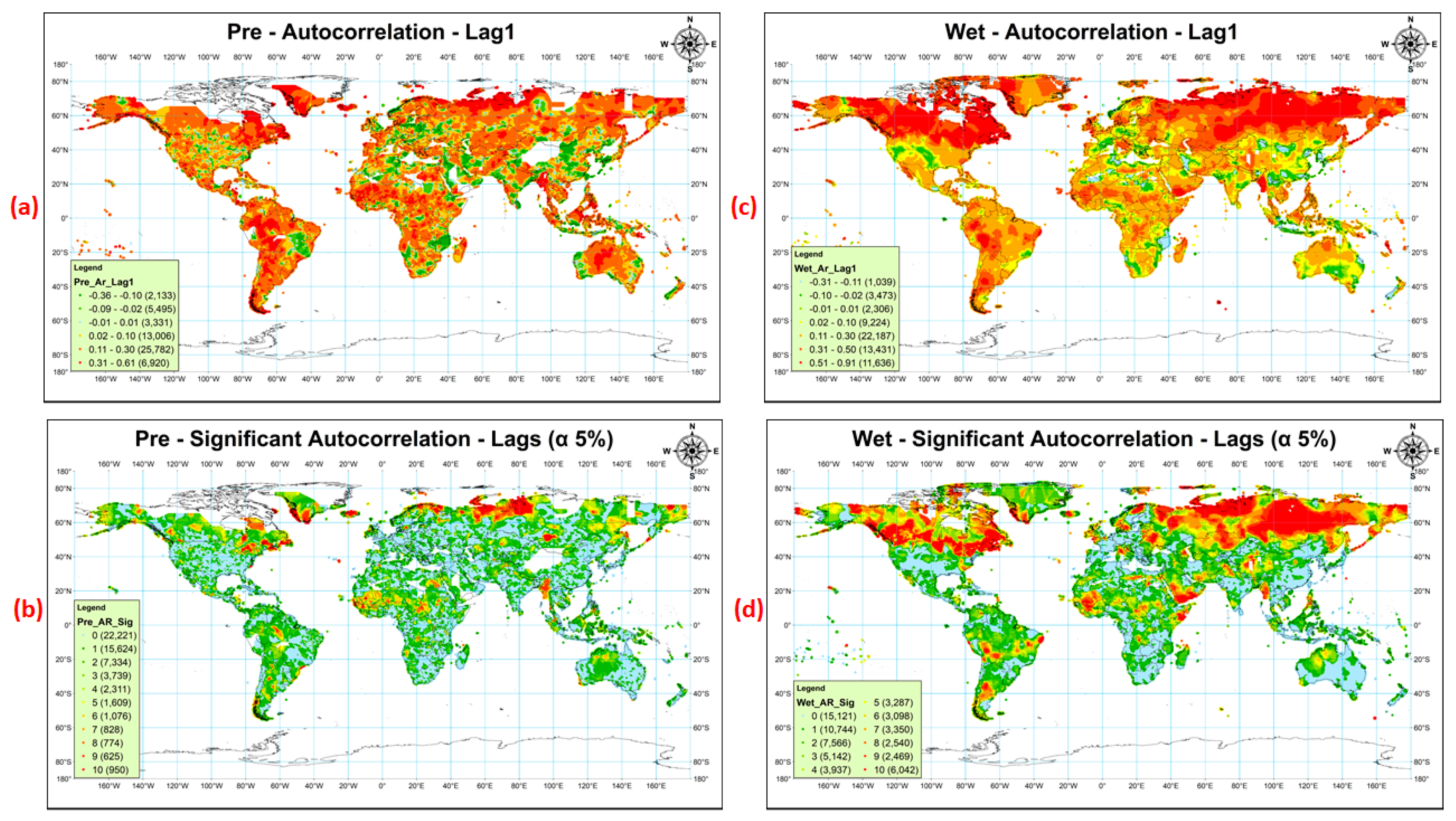
The lag1 autocorrelation, the significant autocorrelations up to lag10 at 5% significant level for Pre and Wet are shown in Figure 1a–d. Only a few of the regions showed significant negative autocorrelation. More than 60% of locations showed significant positive autocorrelation for precipitation, and out of them, almost 70% were found to be significantly autocorrelated up to lag2. Much more regions (>75%) indicated significant serial correlation for Wet data. Far Northern regions showed a higher order of serial correlation than the rest of the world.
So, it can be observed that the majority of the regions are not free from serial correlation. The autocorrelation indicates the persistence in the time series, so the positive serial correlation indicates that the precipitation is following the patterns of previous years in the succeeding years, that is, if the annual precipitation is decreasing, there is a higher probability of it to be decreasing in coming years as well and vice-versa [67,68]. However, this statement cannot be fully justified by observing only serial correlation, so the trends magnitude, direction, and significance were computed.
3.2. Trends
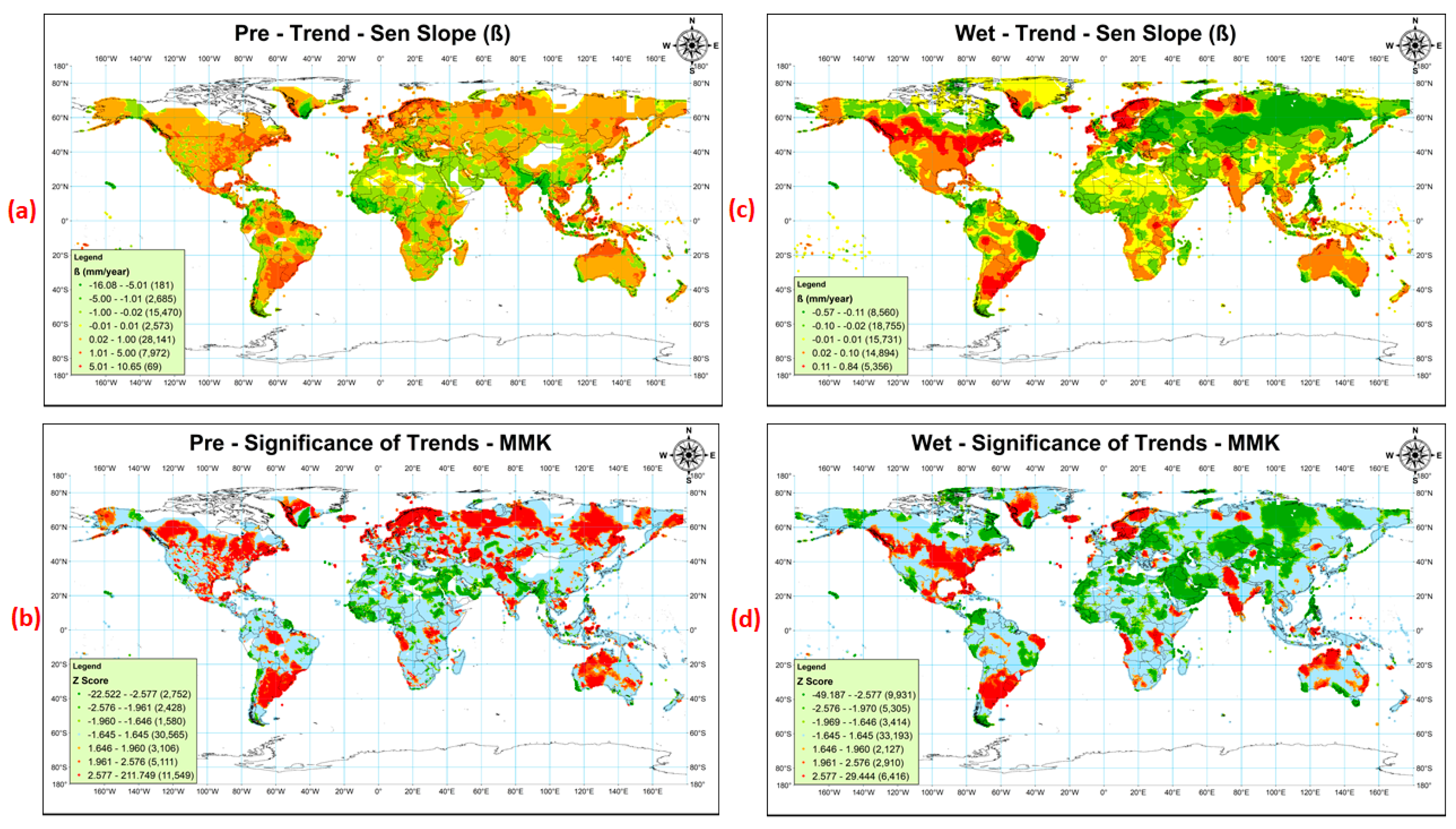
Instead of computing least-square-linear trend using simple linear regression, median slopes were calculated using Sen Slope method as the later one is robust to outliers. As it was found that the data was serially correlated and thus simple MK test could not be used to estimate the significance of the trends, so the MMK test was used which considers the autocorrelation effect on the significance of trends. The median slope ‘ß’ and Z score ‘Zc’ of the MMK test are shown in Figure 2a–d. The value of |Zc| more than or equal to 2.576, 1.96, and 1.645 indicated the significance level of trends at 1%, 5%, and 10%, respectively.
More than 46% of Pre data showed significant increasing or decreasing trends at 5% significance level, out of which high increasing trend of ~5–11 mm/year was found for ~68% regions. Significant decreasing trend, ~5–16mm/year, was detected for ~13% of entire Pre data. So, Pre was found to be increasing for the majority of the regions. Westra et al. [15] and Chou et al. [69] also indicated a significant increase in annual precipitation for more than two-thirds of the world stations.
Significant decreasing trends of Pre were found in the majority of the regions of world largest deserts, i.e., Sahara at Africa, Arabian at the Middle East, Thar at South Asia, Peruvian and Patagonian at South America, and Great Basin at North America. It might indicate a further decrease in the precipitation in the regions, which already were receiving less precipitation. Similar results for the world arid regions were found in the previous studies [70,71]. The regions of comparatively higher Pre, such as Northern and North-Eastern states of India—Bhutan and Myanmar, were found to be receiving lesser Pre, indicating a change in climate in these regions. However, on the contrary, the Pre was found to be significantly increased in the Great Sandy Simpson desert at Australia. Colder regions of the worlds like Russia, Europe, Central Asia, North America, and some Southern regions of South America were found to be experiencing significantly higher precipitation than past [72]. These results are similar to the model results, which identified the effect of anthropogenic activities on the increase in global mean precipitation at the regions near high latitudes and decrease in sub-tropical latitudes [73,74].
Increase or decrease in Pre alone cannot signify the extreme events until trends of the number of wet days are not closely analyzed with trends of precipitation. It was tried to find the relationship between the trends of Pre and Wet. The trends of Wet (ßWet) and the significance of these trends using MMK test are shown in Figure 2c,d, respectively. The significant trends of Wet were more or less similar to the Pre trends for the majority of the regions. The decreasing trend of Wet was found mostly in the regions of Africa, Asia, Russia, and Europe, and increasing trends were detected in some regions of North and South America, Australia, some parts of Europe, and some regions of South Asia. Lucero et al. [75] also found increasing wet days in Argentina (South America), but no change was detected in daily rainfall. However, opposite trends of Wet with Pre were found in the regions of North and East Asia. The Pre was found to be increasing, while the frequency of wet days was detected to be decreasing. This suggests the increase in high magnitude precipitation spells and decrease in the wet season.
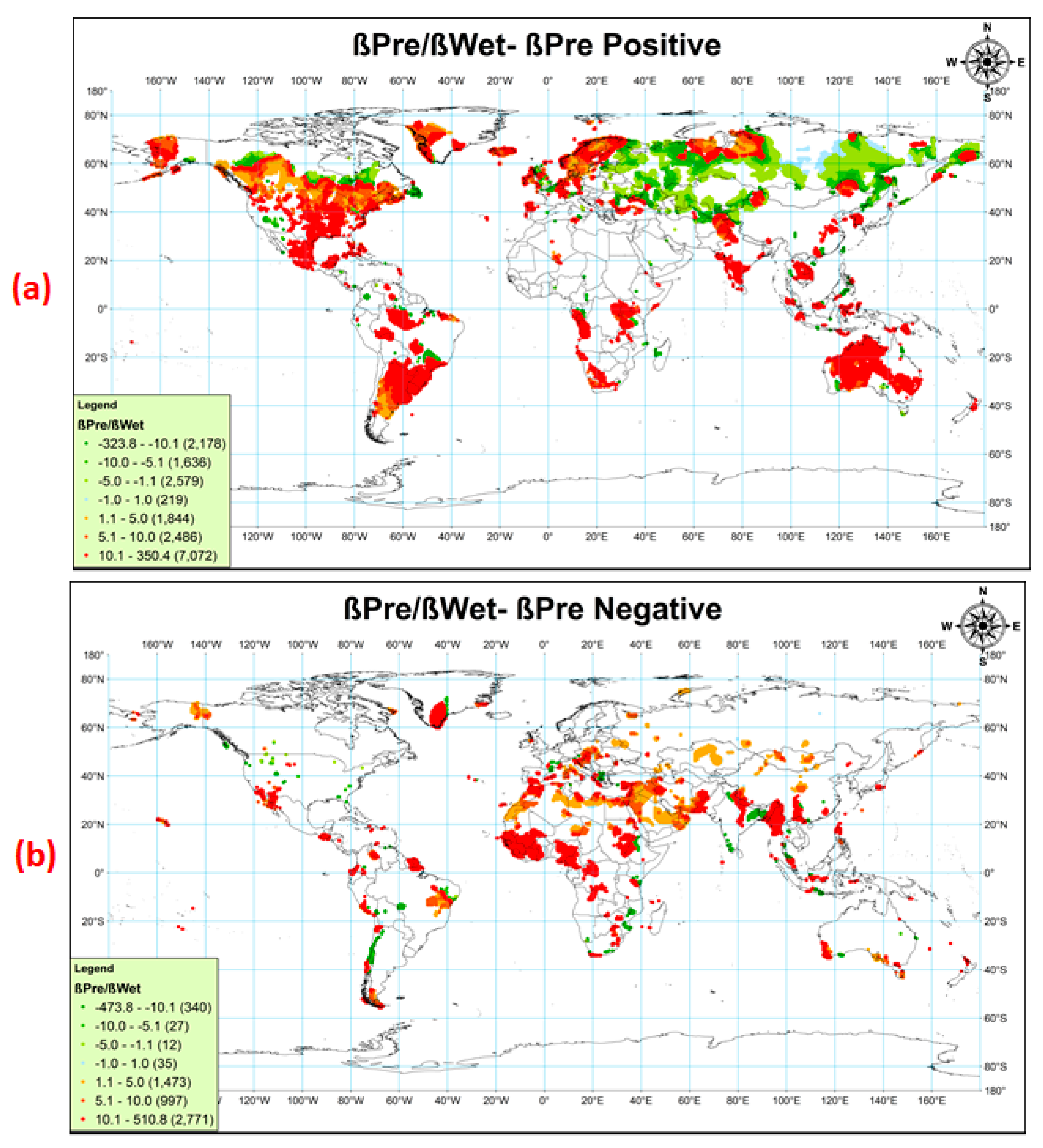
The ratio of the trend of Pre to the trend of Wet shows the change in Pre with a unit change in Wet. Different possible combinations of Pre and Wet were made to analyze the results. These combinations were divided into two major sets, (i) Pre increasing and (ii) Pre decreasing. These major sets were further divided into four possible cases based on the magnitude and sign of ßPre/ßWet.
Case-1 −1 ≤ ßPre/ßWet ≤ 0
Case-2 0 ≤ ßPre/ßWet ≤ 1
Case-3 ßPre/ßWet < −1
Case-4 ßPre/ßWet > 1
Case-1 and 2 indicate that the magnitude of ßPre is lower than the magnitude of ßWet. As the trends of Wet were between −0.57 to 0.84 days/years, the trend of Pre lower than ßWet was found to be insignificant for most of the regions at 10% significance level, so these cases were not presented and discussed in this article. The variation of a trend in Pre with trends of Wet is shown in Figure 3a,b.
3.2.1. Pre Increasing (ßPre > 0)
The ratio of trends, i.e., ßPre/ßWet, is shown in Figure 3a. Case-3 and 4 are presented by shades of green and red color, respectively. The regions with dark green color represent a higher rate of increase in Pre and moderate rate of decrease in Wet, suggesting an increase in the high-intensity precipitation events. The regions with the high increasing trend with moderate or low increasing Wet are shown by dark red color, indicating moderate to the high intensity of precipitation events. Most of the regions of Russia, Central Asia, and Southern Canada were found to be experiencing a higher intensity of Pre events and longer duration of the dry season.
3.2.2. Pre Decreasing (ßPre < 0)
The ratio of trends, ßPre/ßWet, for the regions, which indicated a decrease in Pre at significance level ≤10%, is shown in Figure 3b. Regions showing a high decrease in precipitation with low to moderate increase in wet-day frequency are shown by dark green color. These regions indicate a slightly higher number of wet spells with low intensity of rainfall. The regions represented by dark red color denotes a high decrease in precipitation with low to moderate decrease in the number of wet days, indicating drier season and wet season with lesser precipitation. These climatic conditions may impose drought-like situations. Some regions of South-East Asia, i.e., Myanmar, North India, Afghanistan, East and Central Africa, and some coastal regions of Australia, North and South America were found to be receiving a much lesser amount of precipitation with lesser number of wet spells.
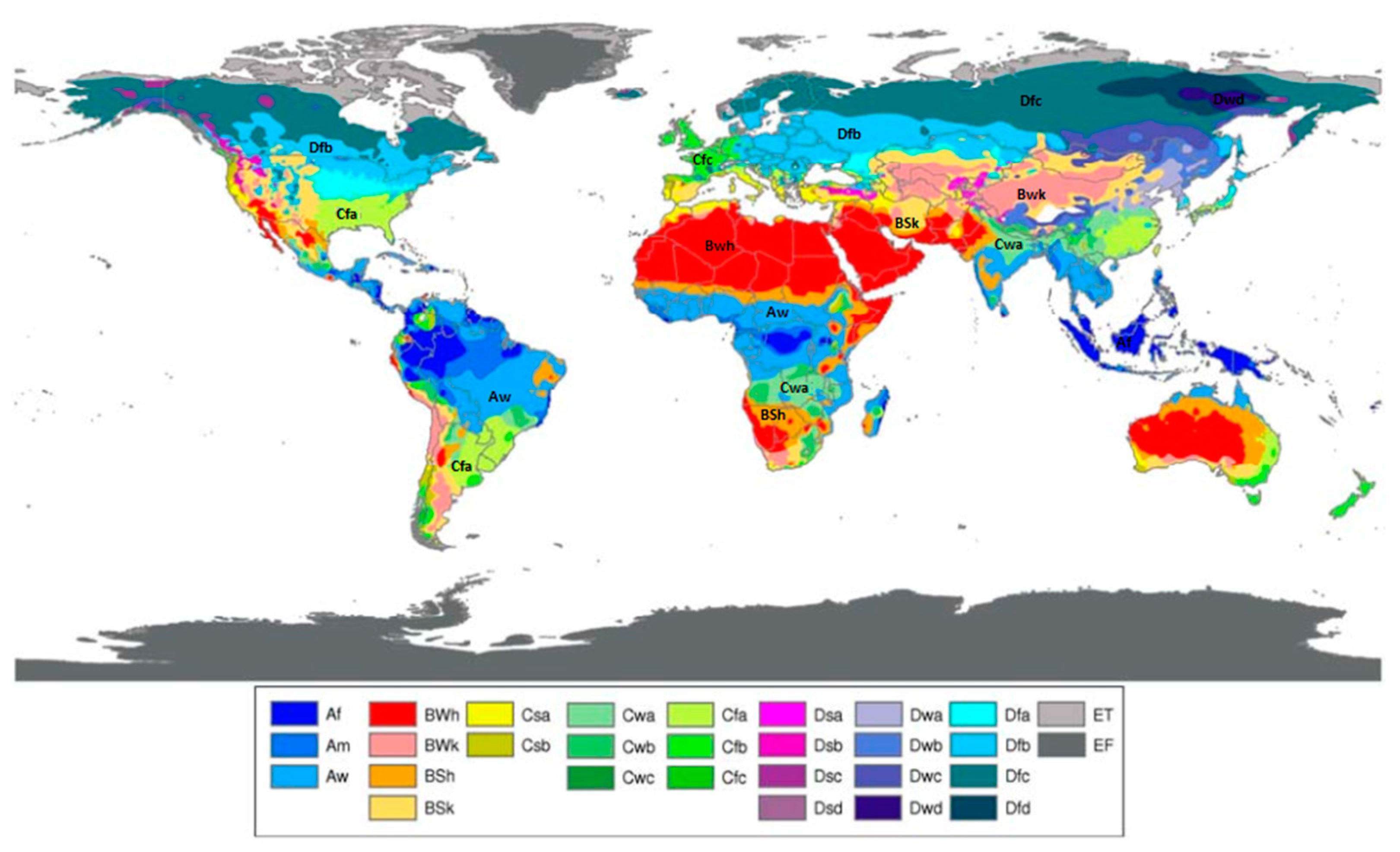
It was also tried to find the relationship between Pre trends in different climates of the world. Different climate types of the world [45] are shown in Figure 4.
The falling trend of Pre for climate class ‘BWh’ (represents Arid ‘B’, desert ‘W’, and hot climate ‘h’ type) at 10% significance level was detected except for Australia where an increase in Pre was detected. This climate type represents the deserts having much lesser Pre, so the regions of North Africa, Middle East, and South Asia have started receiving lesser precipitation, and the chances of drought events might get an increase. However, the dry regions of Australia were found to be receiving higher precipitation. The first letter ‘D’ of the climate class was defined by a cold climate with a temperature of the hottest month ≥10 °C and the temperature of the coldest month ≤0 °C. The second letter ‘f’ represent regions without dry seasons and the third letter a, b, c, d represents hot, warm, cold summer and very cold winter respectively. More than 70% of cold climate type regions without dry seasons, i.e., ‘Dfa’, ‘Dfb’, ‘Dfc’, and ‘Dfd’, showed increasing Pre trends at 1% significance level. So, the cold regions started to be receiving comparatively higher precipitation. The first letter ‘C’ of climate type represents temperate climate, which was defined by the temperature of the hottest month ≥18 °C and the temperature of the coldest month between 0 °C–18 °C. Decreasing trends in the Pre were found for temperate regions, which receives comparatively lesser rainfall than other temperate regions, i.e., climate type ‘Cwa’ (‘w’ for dry winter and ‘a’ for hot summer). Tropical climate type was represented by the first letter ‘A’ and defined by coldest month temperature ≥18 °C. Decreasing trends of Pre were found at a 5% significance level for most of the Tropical Savannah regions characterized by ‘Aw’, which receives comparatively lesser dry season rainfall.
Generally, it has been found that the regions with high magnitude of increasing trends are more prone to high-intensity precipitation spells and the regions with high magnitude of decreasing trends are highly susceptible to receive much lesser precipitation and longer dry seasons. These findings are fulfilling the criteria of rainfall intensification defined by [34], which refers to the more extreme climate of longer dry spells and more extreme rainfall.
3.3. Best-Fit Distribution
Three most popular goodness of fit (GoF) tests, i.e., AD, KS, and CS test, were applied to find the best-fit probability distributions. A significance level of 5% was adopted in this study for GoF tests. AD test is considered to be best a suitable GoF test because it gives more weights to the tails of the distribution [76]. CS test is not considered to be high power GoF test [77]. A summary of the percentage of precipitation data best fitted for a particular probability distribution is given in Table 2. Best-fit probability distributions for annual precipitation data for the landmass of the world is shown in Figure 5.
Almost entire Madagascar was found to be best fitted with Log-Logistic (LL) distribution. GEV, Generalized-Logistic (GL), and LL distributions were best fitted to more than 68% regions of the world for precipitation data. GEV distribution was mostly best fitted in regions of North America, Russia, Europe, India, and Eastern China. Most of the regions of Northern and Eastern Russia, Mongolia, Northern and Central China, Bangladesh, Indonesia, Middle East, Madagascar, Central Africa, Northern South and North America, and Northern Greenland showed more similarity with GL and LL distributions.
The best-fit distributions for different regions showed significant changes in precipitation patterns that might be divided into two groups.
3.3.1. Regions with Significant Decreases in Annual Precipitation
Pre patterns for the arid lands of North Africa showed similarity with GEV and GL distributions. The regions of the Middle East showed agreement with the GL and LL distributions. GL distribution was found to be the best fit for eastern regions of India and Myanmar. Regions of Greenland and South America showing significant decreasing trend were found to follow the frequency of GEV distribution.
3.3.2. Regions with Significant Increases in Annual Precipitation
Most of the mid to high latitude regions showed significant increasing trends in annual Pre. These regions were found to be the best fit with GEV and Generalized Gamma (GG) distributions. High latitude regions of Southern hemisphere were found to be showing similarity with GEV, GG, and LL distributions.
4. Discussion
The hydrological cycle is changing due to climate change at a global scale, and the precipitation is one of the most vulnerable hydrometeorological variable [78]. In this study, a net increase in total annual precipitation for the last century was observed in more than two-third landmasses of the world, supporting the findings of other previous studies [15,69]. However, large variations in the seasonal patterns were observed, including shifting of monsoon season [79], increase in the frequency of extreme events, i.e., floods, droughts, etc. [28,80]. The present study also indicated a decrease in moderate precipitation events and an increase in extreme precipitation with a decreasing number of rainfall events, leading to the long spell of dry summers and short spell of the high rainfall season. However, the inference of “dry become drier and wet become wetter” [73,81] could not be justified in the present study, as some arid regions showed an increase in the precipitation events (arid regions in Australia), while others showed an increase in the desert land, supporting the findings of Greve et al. [82].
As long-term prediction of rainfall data is not feasible deterministically, the assumed probability distribution functions are fitted to find the magnitude and/or frequency of precipitation [83]. The prediction of precipitation is required for efficient water-resource management and to optimize the infrastructure designs. A wide range of PDF was adopted, in this study, to find the distribution which might best describe the precipitation. GEV, LL, and GL PDFs were best fitted to more than two-thirds of the locations, indicating that these distributions might be adopted for annual rainfall predictions rather than general events. Similar studies also indicate that the GEV distribution may be the best choice for the representation of precipitation [84]. It is recommended to find the best-fit distribution among a variety of PDFs to predict the rainfall at a local scale. The findings of this study are limited to only annual total precipitation, which may differ if the temporal scale is changed, such as daily, seasonal, extreme events, etc.
5. Conclusions
The present study assessed the changes in annual Pre patterns and found the simple probability model that could best describe the annual Pre patterns in different Koppen-Giger world climate types across the globe. Based on this study, the following can be inferred:
- The relationship of the trends of Pre with Wet showed an increase in the intensity of Pre and longer duration of dry seasons for most of the cold regions in mid to high latitude regions.
- Drought-like conditions, i.e., low-intensity wet spells and long dry spells, were found to be prevailing in the arid and semi-arid regions of the world.
- The best-fit probability distribution for the regions showing significant decrease or increase (at a 5% significance level) in annual Pre indicated that GL and GEV distributions were two competent models followed by LL distribution.
- Widely considered probability distributions by different climatologists, i.e., Gamma, Log-Normal, Extreme Value and 3, and Generalized Pareto distributions, were best fitted to less than 1% (individually) of global regions, while Normal and Log-Pearson 3 distributions best fitted to 2–5% regions only. So, the authors conclude that instead of simply assuming the probability distribution for statistical analysis and forecasting long-term precipitation at any location of the world, either a wide range of PDFs should be fitted to data to find the best-fit PDF or simply the results of this study may be referred.
This study may be helpful for not only the researchers but also planners to predict the annual behavior of precipitation patterns across the globe, and this could help in designing the economic infrastructure and saving lives.
Author Contributions
In this research work, data collection, their analysis, and manuscript preparation were carried out by C.S. under the supervision of C.S.P.O. His expert advice and review helped in improving the paper.
Funding
This research received no external funding.
Acknowledgments
The authors are thankful to Climatic Research Unit (CRU) for providing the gridded precipitation and wet-day frequency data. The authors would like to thank Indian Institute of Technology, Roorkee, India for providing funding support for APC from Institute Chair-professor fund of second author C.S.P. Ojha. The authors are also thankful for the computational resources provided by the NERC, United Kingdom (Project NE/N016394/1)—“Sustaining Himalaya Water Resources in a Changing Climate (SusHi-Wat)” —as part of the UK-India Newton-Bhabha Sustainable Water Resources (SWR) thematic programme.
Conflicts of Interest
The authors declare no conflict of interest.
Appendix A. PDF of Distributions
For a time series , where n represents the number of data points in the time series
Appendix A.1. Generalized Gamma, Generalized Gamma_F, Gamma and Gamma_F
Four-Parameter Generalized Gamma distribution PDF is given by
here, k, α, β and γ are shape, shape, scale, and location parameters, respectively.
Special Cases:
- γ = 0 yields three-parameter Generalized Gamma distribution, Generalized Gamma_F
- k = 1 yields three-Parameter Gamma Distribution
- γ = 0 and k = 1 yields two-parameter Gamma distribution, Gamma_F
Appendix A.2. Generalized Extreme Value Distribution (GEV)
Appendix A.3. Gumbel Max and Gumbel Min
Gumbel Distribution is a special case of Generalized Extreme Value Distribution with parameter k = 0
Appendix A.4. Generalized Logistic Distribution (GL)
Appendix A.5. Log-Logistic and Log-Logistic_F
Appendix A.6. Normal
Appendix A.7. Lognormal and Lognormal_F
Appendix A.8. Log-Pearson Type III
Appendix A.9. Pearson-5 and Pearson-5_F
Appendix A.10. Pearson-6 and Pearson-6_F
Appendix A.11. Weibull and Weibull_F
Appendix B. Parameter Estimation Methods
Appendix B.1. Method of Least-Squares (LS)
For a time series , where n represents the number of data points in the time series, a probability distribution, whose cumulative distribution function (CDF) is given by F(θ), is being fitted. Let are the parameters of the fitted probability distribution. To estimate the values of parameters, the squared difference of theoretical and empirical CDF is minimized.
The empirical cumulative distribution function (ECDF) is defined as
here, is rank of variable, is arranged in ascending order, and N is the total number of data points in time series.
The error between theoretical and empirical CDF is given by
Minimization of the error gives the best choice of the fitted distribution parameters. Partial derivatives of the error with respect to each parameter generate different sets of equations. These equations are used to find the distribution parameters.
Appendix B.2. Maximum Likelihood Method (ML)
The principle of maximum likelihood says that for a given dataset, find the model parameter(s) in such a way that dataset is most likely. The likelihood of true model parameters (given the data set) is the same as the probability of getting the data given the true model parameter value.
here L is the likelihood of parameter , and is the product of probabilities of getting .
Equating the partial derivative of the likelihood function (with respect to each parameter ) to zero gives the model parameters values.
Maximization of likelihood function gives the best model parameter. As it is difficult to maximize the likelihood function, so maximization of log-likelihood is done.
Appendix B.3. Method of Moments (Mo)
In this method, the parameters are estimated by equating sample and theoretical moments.
is the kth theoretical moment of the distribution about the mean, k = 1, 2…
is the kth sample moment about the mean, k = 1, 2…
First, second, third, and higher-order sample moments are equated to respected higher-order theoretical moments until we get the required number of equations to estimate the parameters. Parameters values for different distributions are estimated by solving the equations [86].
Appendix B.4. Method of L-Moments (LMo)
Appendix C. Goodness of Fit Tests
The goodness of fit tests measure the closeness of fitted distribution to the data with a theoretical probability distribution. Following three goodness of fit tests are most commonly used:
Appendix C.1. Anderson–Darling Test (AD Test)
The AD test compares the observed CDF of the data with expected CDF for a particular probability distribution. This test is powerful than the KS test because it gives more weights to the tails. The AD Test statistic (A2) is
The null hypothesis (H0) for the test states that the data follow the particular distribution, and the alternate hypothesis defines that the data don’t follow the specified distribution. The null hypothesis is rejected if the test is a statistic, and A2 is greater than the critical value at a defined significance level α.
Appendix C.2. Kolmogorov–Smirnov Test (KS Test)
This test measures the largest vertical distance between empirical CDF (ECDF) of the data and the theoretical CDF of the particular distribution. For a time series, where n represents the number of data points in time series, the ECDF is given by
The KS test statistic (D) is defined as
The null hypothesis (H0) states that the data follow the specified distribution. The null hypothesis is rejected if D is greater than the critical value at a defined significance level.
Appendix C.3. Chi-Squared Test (CS Test)
This test compares the observed frequency () of the data with expected frequency () of the particular distribution at different bins. The CS test statistic is defined as
here, are CDF values of the particular probability distribution for a bin limit .
The null hypothesis (H0) states that the data follow the specified distribution. The null hypothesis is rejected if value is more extreme than the critical value of at a specified significance level. The critical value of is found from the standard tables of for specified significance levels and k − 1 degrees of freedom.
The data can be binned into groups of equal probability or equal width. The former approach is better since it handles the peak data effectively. This test is not considered a high power statistical test for goodness of fit [77].
References
- Stocker, T.; Qin, D.; Plattner, G.K.; Tignor, M.; Allen, S.; Boschung, J.; Midgley, P. Summary for Policymakers. In Climate Change 2013: The Physical Science Basis. Contribution of Working Group I to the IPCC Fifth Assessment Report of the Intergovernmental Panel on Climate Change; IPCC: Cambridge, UK; New York, NY, USA, 2013. [Google Scholar]
- Donat, M.G.; Lowry, A.L.; Alexander, L.V.; O’Gorman, P.A.; Maher, N. More extreme precipitation in the world’s dry and wet regions. Nat. Clim. Chang. 2016, 6, 508–513. [Google Scholar] [CrossRef]
- Lehmann, J.; Coumou, D.; Frieler, K. Increased record-breaking precipitation events under global warming. Clim. Chang. 2015, 132, 501–515. [Google Scholar] [CrossRef]
- Mishra, V.; Ganguly, A.R.; Nijssen, B.; Lettenmaier, D.P. Changes in observed climate extremes in global urban areas. Environ. Res. Lett. 2015, 10, 024005. [Google Scholar] [CrossRef]
- Biskaborn, B.K.; Smith, S.L.; Noetzli, J.; Matthes, H.; Vieira, G.; Streletskiy, D.A.; Schoeneich, P.; Romanovsky, V.E.; Lewkowicz, A.G.; Abramov, A.; et al. Permafrost is warming at a global scale. Nat. Commun. 2019, 10, 264. [Google Scholar] [CrossRef] [PubMed]
- Gudmundsson, L.; Leonard, M.; Do, H.X.; Westra, S.; Seneviratne, S.I. Observed Trends in Global Indicators of Mean and Extreme Streamflow. Geophys. Res. Lett. 2018, 46, 756–766. [Google Scholar] [CrossRef]
- Sen, P.K. Estimates of the Regression Coefficient Based on Kendall’s Tau. J. Am. Stat. Assoc. 1968, 57, 269–306. [Google Scholar] [CrossRef]
- Jain, S.K.; Kumar, V. Trend analysis of rainfall and temperature data for India. Curr. Sci. 2012, 102, 37–49. [Google Scholar] [CrossRef]
- Bera, S. Trend Analysis of Rainfall in Ganga Basin, India during 1901–2000. Am. J. Clim. Chang. 2017, 6, 116–131. [Google Scholar] [CrossRef]
- Duhan, D.; Pandey, A. Statistical analysis of long term spatial and temporal trends of precipitation during 1901–2002 at Madhya Pradesh, India. Atmos. Res. 2013, 122, 136–149. [Google Scholar] [CrossRef]
- Mann, H.B. Nonparametric Tests Against Trend. Econometrica 1945, 13, 245–259. [Google Scholar] [CrossRef]
- Kendall, M.G. Rank Correlation Methods, 4th ed.; Charless Griffin: London, UK, 1975; ISBN 0195208374. [Google Scholar]
- Modarres, R.; Sarhadi, A. Rainfall trends analysis of Iran in the last half of the twentieth century. J. Geophys. Res. Atmos. 2009, 114, 1–9. [Google Scholar] [CrossRef]
- Pranuthi, G.; Dubey, S.K.; Tripathi, S.K.; Chandniha, S.K. Trend and Change Point Detection of Precipitation in Urbanizing Districts of Uttarakhand in India. Indian J. Sci. Technol. 2014, 7, 1573–1582. [Google Scholar]
- Westra, S.; Alexander, L.V.; Zwiers, F.W. Global increasing trends in annual maximum daily precipitation. J. Clim. 2013, 26, 3904–3918. [Google Scholar] [CrossRef]
- Villarini, G.; Serinaldi, F.; Smith, J.A.; Krajewski, W.F. On the stationarity of annual flood peaks in the continental United States during the 20th century. Water Resour. Res. 2009, 45, 1–17. [Google Scholar] [CrossRef]
- Sharma, C.; Arora, H.; Ojha, C.S.P. Assessment of the Effect of Climate Change on Historical and Future Rainfall in Uttarakhand. In Proceedings of the Hydro-2015 International, Roorkee, India, 17–19 December 2015. [Google Scholar] [CrossRef]
- Yue, S.; Pilon, P.; Cavadias, G. Power of the Mann-Kendall and Spearman’s rho tests for detecting monotonic trends in hydrological series. J. Hydrol. 2002, 259, 254–271. [Google Scholar] [CrossRef]
- Hamilton, J.P.; Whitelaw, G.S.; Fenech, A. Mean Annual Temperature and Total Annual Precipitation Trends at Canadian Biosphere Reserves. Environ. Monit. Assess. 2001, 67, 239–275. [Google Scholar] [CrossRef]
- Burn, D.H.; Hag Elnur, M.A. Detection of hydrologic trends and variability. J. Hydrol. 2002, 255, 107–122. [Google Scholar] [CrossRef]
- Gocic, M.; Trajkovic, S. Analysis of changes in meteorological variables using Mann-Kendall and Sen’s slope estimator statistical tests in Serbia. Glob. Planet. Chang. 2013, 100, 172–182. [Google Scholar] [CrossRef]
- Bayazit, M.; Önöz, B. To prewhiten or not to prewhiten in trend analysis? Hydrol. Sci. J. 2007, 52, 611–624. [Google Scholar] [CrossRef]
- Yue, S.; Pilon, P.; Phinney, B.; Cavadias, G. The influence of autocorrelation on the ability to detect trend in hydrological series. Hydrol. Process. 2002, 16, 1807–1829. [Google Scholar] [CrossRef]
- Hamed, K.H.; Ramachandra Rao, A. A modified Mann-Kendall trend test for autocorrelated data. J. Hydrol. 1998, 204, 182–196. [Google Scholar] [CrossRef]
- Wahl, T.; Jain, S.; Bender, J.; Meyers, S.D.; Luther, M.E. Increasing risk of compound flooding from storm surge and rainfall for major US cities. Nat. Clim. Chang. 2015, 5, 1093–1097. [Google Scholar] [CrossRef]
- Sinha, D.; Syed, T.H.; Famiglietti, J.S.; Reager, J.T.; Thomas, R.C. Characterizing Drought in India Using GRACE Observations of Terrestrial Water Storage Deficit. J. Hydrometeorol. 2017, 18, 381–396. [Google Scholar] [CrossRef]
- Luo, M.; Lau, N.C. Synoptic characteristics, atmospheric controls, and long-term changes of heat waves over the Indochina Peninsula. Clim. Dyn. 2018, 51, 2707–2723. [Google Scholar] [CrossRef]
- Coumou, D.; Rahmstorf, S. A decade of weather extremes. Nat. Clim. Chang. 2012, 2, 491–496. [Google Scholar] [CrossRef]
- Sippel, S.; Zscheischler, J.; Heimann, M.; Lange, H.; Mahecha, M.D.; van Oldenborgh, G.J.; Otto, F.E.L.; Reichstein, M. Have precipitation extremes and annual totals been increasing in the world’s dry regions over the last 60 years? Hydrol. Earth Syst. Sci. 2017, 21, 441–458. [Google Scholar] [CrossRef]
- Zhang, X.; Zwiers, F.W.; Hegerl, G.C.; Lambert, F.H.; Gillett, N.P.; Solomon, S.; Stott, P.A.; Nozawa, T. Detection of human influence on twentieth-century precipitation trends. Nature 2007, 448, 461–465. [Google Scholar] [CrossRef]
- Feng, X.; Liu, C.; Xie, F.; Lu, J.; Chiu, L.S.; Tintera, G.; Chen, B. Precipitation Characteristic Changes due to Global Warming in a High-Resolution (16-km) ECMWF Simulation. Q. J. R. Meteorol. Soc. 2018, 1–15. [Google Scholar] [CrossRef]
- Choi, G.; Collins, D.; Ren, G.; Trewin, B.; Baldi, M.; Fukuda, Y.; Afzaal, M.; Pianmana, T.; Gomboluudev, P.; Huong, P.T.T.; et al. Changes in means and extreme events of temperature and precipitation in the Asia-Pacific Network region, 1955–2007. Int. J. Climatol. 2009, 29, 1906–1925. [Google Scholar] [CrossRef]
- Goyal, M.K.; Gupta, V. Identification of homogeneous rainfall regimes in northeast region of India using fuzzy cluster analysis. Water Resour. Manag. 2014, 28, 4491–4511. [Google Scholar] [CrossRef]
- Giorgi, F.; Im, E.S.; Coppola, E.; Diffenbaugh, N.S.; Gao, X.J.; Mariotti, L.; Shi, Y. Higher hydroclimatic intensity with global warming. J. Clim. 2011, 24, 5309–5324. [Google Scholar] [CrossRef]
- Raghavendra, A.; Zhou, L.; Jiang, Y.; Hua, W. Increasing extent and intensity of thunderstorms observed over the Congo Basin from 1982 to 2016. Atmos. Res. 2018, 213, 17–26. [Google Scholar] [CrossRef]
- Choudhury, B.A.; Saha, S.K.; Konwar, M.; Sujith, K.; Deshamukhya, A. Rapid Drying of Northeast India in the Last Three Decades: Climate Change or Natural Variability? J. Geophys. Res. Atmos. 2019, 124, 227–237. [Google Scholar] [CrossRef] [Green Version]
- Thomas, N.; Nigam, S. Twentieth-century climate change over Africa: Seasonal hydroclimate trends and sahara desert expansion. J. Clim. 2018, 31, 3349–3370. [Google Scholar] [CrossRef]
- Alexander, L.V.; Zhang, X.; Peterson, T.C.; Caesar, J.; Gleason, B.; Klein Tank, A.M.G.; Haylock, M.; Collins, D.; Trewin, B.; Rahimzadeh, F.; et al. Global observed changes in daily climate extremes of temperature and precipitation. J. Geophys. Res. 2006, 111, D05109. [Google Scholar] [CrossRef]
- Rajeevan, M.; Bhate, J.; Jaswal, A.K. Analysis of variability and trends of extreme rainfall events over India using 104 years of gridded daily rainfall data. Geophys. Res. Lett. 2008, 35, 1–6. [Google Scholar] [CrossRef]
- Köppen, W. The thermal zones of the Earth according to the duration of hot, moderate and cold periods and to the impact of heat on the organic world. Meteorol. Z. 2011, 20, 351–360. [Google Scholar] [CrossRef]
- Hanf, F.; Körper, J.; Spangehl, T.; Cubasch, U. Shifts of climate zones in multi-model climate change experiments using the Köppen climate classification. Meteorol. Z. 2012, 21, 111–123. [Google Scholar] [CrossRef]
- Chen, D.; Chen, H.W. Using the Köppen classification to quantify climate variation and change: An example for 1901–2010. Environ. Dev. 2013, 6, 69–79. [Google Scholar] [CrossRef]
- Gao, X.; Giorgi, F. Increased aridity in the Mediterranean region under greenhouse gas forcing estimated from high resolution simulations with a regional climate model. Glob. Planet. Chang. 2008, 62, 195–209. [Google Scholar] [CrossRef]
- Kottek, M.; Grieser, J.; Beck, C.; Rudolf, B.; Rubel, F. World Map of the Köppen-Geiger climate classification updated. Meteorol. Z. 2006, 15, 259–263. [Google Scholar] [CrossRef]
- Peel, M.C.; Finlayson, B.L.; McMahon, T.A. Updated world map of the Köppen-Geiger climate classification. Hydrol. Earth Syst. Sci. 2007, 11, 1633–1644. [Google Scholar] [CrossRef]
- Beck, H.E.; Zimmermann, N.E.; McVicar, T.R.; Vergopolan, N.; Berg, A.; Wood, E.F. Present and future köppen-geiger climate classification maps at 1-km resolution. Sci. Data 2018, 5, 180214. [Google Scholar] [CrossRef] [PubMed]
- Ye, L.; Hanson, L.S.; Ding, P.; Wang, D.; Vogel, R.M. The Probability Distribution of Daily Precipitation at the Point and Catchment Scales in the United States. Hydrol. Earth Syst. Sci. Discuss. 2018, 22, 1–28. [Google Scholar] [CrossRef]
- Blain, G.C.; Meschiatti, M.C. Using multi-parameters distributions to assess the probability of occurrence of extreme rainfall data. Rev. Bras. Eng. Agríc. Ambient. 2014, 18, 307–313. [Google Scholar] [CrossRef] [Green Version]
- Douka, M.; Karacostas, T. Statistical analyses of extreme rainfall events in Thessaloniki, Greece. Atmos. Res. 2018, 208, 60–77. [Google Scholar] [CrossRef]
- Santos, E.B.; Lucio, P.S.; Santos e Silva, C.M. Estimating return periods for daily precipitation extreme events over the Brazilian Amazon. Theor. Appl. Climatol. 2016, 126, 585–595. [Google Scholar] [CrossRef]
- Papalexiou, S.M.; Koutsoyiannis, D. A global survey on the seasonal variation of the marginal distribution of daily precipitation. Adv. Water Resour. 2016, 94, 131–145. [Google Scholar] [CrossRef]
- Papalexiou, S.M.; Koutsoyiannis, D. Battle of extreme value distributions: A global survey on extreme daily rainfall. Water Resour. Res. 2013, 49, 187–201. [Google Scholar] [CrossRef]
- Papalexiou, S.M.; Koutsoyiannis, D. Entropy based derivation of probability distributions: A case study to daily rainfall. Adv. Water Resour. 2012, 45, 51–57. [Google Scholar] [CrossRef]
- Harris, I.; Jones, P.D.; Osborn, T.J.; Lister, D.H. Updated high-resolution grids of monthly climatic observations—The CRU TS3.10 Dataset. Int. J. Climatol. 2014, 34, 623–642. [Google Scholar] [CrossRef]
- Mitchell, T.D.; Jones, P.D. An improved method of constructing a database of monthly climate observations and associated high-resolution grids. Int. J. Climatol. 2005, 25, 693–712. [Google Scholar] [CrossRef]
- New, M.; Hulme, M.; Jones, P. Representing Twentieth-Century Space–Time Climate Variability. Part II: Development of 1901–96 Monthly Grids of Terrestrial Surface Climate. J. Clim. 2000, 13, 2217–2238. [Google Scholar] [CrossRef]
- Ming, J.; Sun, J. Enhancement of the relationship between boreal summer precipitation over eastern China and Australia since the early 1980s. Int. J. Climatol. 2019, 39, 266–277. [Google Scholar] [CrossRef]
- Chen, J.; Brissette, F.P. Reliability of climate model multi-member ensembles in estimating internal precipitation and temperature variability at the multi-decadal scale. Int. J. Climatol. 2019, 39, 843–856. [Google Scholar] [CrossRef]
- Knoben, W.J.M.; Woods, R.A.; Freer, J.E. Global bimodal precipitation seasonality: A systematic overview. Int. J. Climatol. 2019, 39, 558–567. [Google Scholar] [CrossRef]
- Sharma, C.; Ojha, C.S.P. Statistical Parameters of Hydrometeorological Variables: Standard Deviation, SNR, Skewness and Kurtosis. In Advances in Water Resources Engineering and Management; Springer: Singapore, 2019; Volume I, p. 257. ISBN 9811381801. [Google Scholar]
- Udo, M.S.; Andreas, B.; Peter, F.; Meyer-Christoffer, A.; Bruno, R.; Ziese, M. GPCC Full Data Reanalysis Version 6.0 at 0.5°: Monthly Land-Surface Precipitation from Rain-Gauges Built on GTS-Based and Historic Data; Global Precipitation Climatology Centre (GPCC): Berlin, Germany, 2011. [Google Scholar] [CrossRef]
- Brockwell, P.J.; Davis, R.A. Introduction to Time Series and Forecasting; Springer: New York, NY, USA, 2002; ISBN 0387953515. [Google Scholar]
- El-Shaarawi, A.H.; Piegorsch, W.W. Encyclopedia of Environmetrics; Wiley: New York City, NY, USA, 2002; Volume 1, ISBN 0471899976. [Google Scholar]
- Greenwood, J.A.; Landwehr, J.M.; Matalas, N.C.; Wallis, J.R. Probability weighted moments: Definition and relation to parameters of several distributions expressable in inverse form. Water Resour. Res. 1979, 15, 1049–1054. [Google Scholar] [CrossRef] [Green Version]
- Hosking, J.R.M. L-Moments: Analysis and Estimation of Distributions Using Linear Combinations of Order Statistics. J. R. Stat. Soc. 1990, 52, 105–124. [Google Scholar] [CrossRef]
- Zerda, I. An experimental comparison of popular estimation methods for the Weibull, Gamma and Gompertz Distributions. Schedae Inform. 2012, 20, 67–82. [Google Scholar] [CrossRef]
- Giles, B.D.; Flocas, A.A. Air temperature variations in Greece. Part 1. Persistence, trend, and fluctuations. J. Climatol. 1984, 4, 531–539. [Google Scholar] [CrossRef]
- Mirza, M.Q.; Warrick, R.A.; Ericksen, N.J.; Kenny, G.J. Trends and persistence in precipitation in the Ganges, Brahmaputra and Meghna river basins. Hydrol. Sci. J. 1998, 43, 845–858. [Google Scholar] [CrossRef]
- Chou, C.; Lan, C.-W. Changes in the Annual Range of Precipitation under Global Warming. J. Clim. 2011, 25, 222–235. [Google Scholar] [CrossRef]
- Liu, Q.; Yang, Z.; Cui, B. Spatial and temporal variability of annual precipitation during 1961–2006 in Yellow River Basin, China. J. Hydrol. 2008, 361, 330–338. [Google Scholar] [CrossRef]
- Caloiero, T.; Coscarelli, R.; Ferrari, E.; Mancini, M. Trend detection of annual and seasonal rainfall in Calabria (Southern Italy). Int. J. Climatol. 2011, 31, 44–56. [Google Scholar] [CrossRef]
- Kiely, G.; Albertson, J.D.; Parlange, M.B. Recent trends in diurnal variation of precipitation at Valentia on the west coast of Ireland. J. Hydrol. 1998, 207, 270–279. [Google Scholar] [CrossRef] [Green Version]
- Held, I.M.; Soden, B.J. Robust responses of the hydrological cycle to global warming. J. Clim. 2006, 19, 5686–5699. [Google Scholar] [CrossRef]
- Vose, R.S.; Schmoyer, R.L.; Steurer, P.M.; Peterson, T.C.; Heim, R.; Karl, T.R.; Eischeid, J.K. The Global Historical Climatology Network: Long-Term Monthly Temperature, Precipitation, Sea Level Pressure, and Station Pressure Data (CONF-930133--2); Oak Ridge National Lab.: Oak Ridge, TN, USA, 1992.
- Lucero, O.A.; Rozas, D. Characteristics of aggregation of daily rainfall in a middle-latitudes region during a climate variability in annual rainfall amount. Atmos. Res. 2002, 61, 35–48. [Google Scholar] [CrossRef]
- Millington, N.; Das, S.; Simonovic, S.P. The Comparison of GEV, Log-Pearson Type 3 and Gumbel Distributions in the Upper Thames River Watershed under Global Climate Models; Department of Civil and Environmental Engineering, The University of Western Ontario: London, ON, Canada, 2011; Volume 77, pp. 1–54. ISBN 978-0-7714-2898-2. [Google Scholar]
- Cunnane, C. Statistical Distributions for Flood Frequency Analysis; WMO-No. 718; Operational Hydrology Report (OHR)- No. 33; American Meteorological Society: Boston, MA, USA, 1989; ISBN 978-92-63-10718-3. [Google Scholar]
- Haddeland, I.; Heinke, J.; Biemans, H.; Eisner, S.; Flörke, M.; Hanasaki, N.; Konzmann, M.; Ludwig, F.; Masaki, Y.; Schewe, J.; et al. Global water resources affected by human interventions and climate change. Proc. Natl. Acad. Sci. USA 2014, 111, 3251–3256. [Google Scholar] [CrossRef]
- Zhisheng, A.; Guoxiong, W.; Jianping, L.; Youbin, S.; Yimin, L.; Weijian, Z.; Yanjun, C.; Anmin, D.; Li, L.; Jiangyu, M.; et al. Global Monsoon Dynamics and Climate Change. Annu. Rev. Earth Planet. Sci. 2015, 43, 29–77. [Google Scholar] [CrossRef] [Green Version]
- O’Gorman, P.A. Precipitation Extremes Under Climate Change. Curr. Clim. Chang. Rep. 2015, 1, 49–59. [Google Scholar] [CrossRef] [Green Version]
- Chou, C.; Neelin, J.D.; Chen, C.-A.; Tu, J.-Y. Evaluating the “Rich-Get-Richer” Mechanism in Tropical Precipitation Change under Global Warming. J. Clim. 2009, 22, 1982–2005. [Google Scholar] [CrossRef]
- Greve, P.; Orlowsky, B.; Mueller, B.; Sheffield, J.; Reichstein, M.; Seneviratne, S.I. Global assessment of trends in wetting and drying over land. Nat. Geosci. 2014, 7, 716–721. [Google Scholar] [CrossRef]
- Papalexiou, S.M.; Koutsoyiannis, D.; Makropoulos, C. How extreme is extreme? An assessment of daily rainfall distribution tails. Hydrol. Earth Syst. Sci. 2013, 17, 851–862. [Google Scholar] [CrossRef] [Green Version]
- Ghosh, S.; Roy, M.K.; Biswas, S.C. Determination of the Best Fit Probability Distribution for Monthly Rainfall Data in Bangladesh. Am. J. Math. Stat. 2016, 6, 170–174. [Google Scholar] [CrossRef]
- Hosking, J.R.M.; Wallis, J.R. Regional Frequency Analysis—An Approach Based on L-Moments; Cambridge University Press: Cambridge, UK, 1997. [Google Scholar] [CrossRef]
- Forbes, C.; Evans, M.; Hastings, N.; Peacock, B. Statistical Distributions, 4th ed.; Wiley: New York City, NY, USA, 2010; ISBN 0470390638. [Google Scholar]
Figure 1.
Lag1 autocorrelation and significant autocorrelation up to lag10 of annual Pre (a,b) and Wet (c,d), respectively. Lag1 autocorrelation for Pre and Wet data (a,c) is divided to show the variation from lower to higher magnitude in either direction. The autocorrelation close to 0 (up to 0.01, positive or negative) is marked by cyan color. The darker shades of the green and red show an increasingly higher amount of negative and positive autocorrelation.

Figure 2.
Sen’s slope trends and its significance using MMK test for Precipitation (a,b) and Wet-day frequency (c,d). The presented trends in subplot (a,c) are divided to represent the magnitude of the trend, that is, the trends close to zero are shown by light shades of green and red (green for decreasing and red for increasing). The darker shade of the green and red color shows higher trend magnitude. The legends of subplots (b,d) are divided according to the significance level of MMK tests, i.e., α = 1, 5, and 10%, standard Z static is ±2.576, ±1.96, and ±1.645, respectively.

Figure 3.
Relative change in trends of Pre with the trend of Wet. (a) Pre trend positive, (b) Pre trend negative. The value of ßPre/ßWet close to unity (indicated by light shades of green and red color) is assumed insignificant as it suggests a lesser amount of Pre trend than Wet. As represented in Figure 2a,c the magnitude of the ßWet is much lesser than ßPre, so the ßPre/ßWet close to unity (also lesser than unity) indicates very small Pre trend.

Figure 4.
Koppen-Geiger climate type map of the landmass of the Earth [45].
Figure 4.
Koppen-Geiger climate type map of the landmass of the Earth [45].

Figure 5.
Best-fit probability distributions for annual precipitation by Anderson–Darling (AD) test. PDF: probability distribution function.
Figure 5.
Best-fit probability distributions for annual precipitation by Anderson–Darling (AD) test. PDF: probability distribution function.


Table 1.
Different Distributions and their parameter estimation methods used in this study.
| Distribution Name | Parameter Estimation Method |
|---|---|
| Gamma | ML |
| Gamma_F | Mo |
| Gen. Extreme Value | LMo |
| Gen. Gamma | ML |
| Gen. Gamma_F | ML |
| Gen. Logistic | LMo |
| Gen. Pareto | LMo |
| Gumbel Max | Mo |
| Gumbel Min | Mo |
| Log-Logistic | ML |
| Log-Logistic_F | LS |
| Log-Pearson 3 | Mo |
| Lognormal | Mo |
| Lognormal_F | Mo |
| Normal | ML |
| Pearson 5 | ML |
| Pearson 5_F | ML |
| Pearson 6 | ML |
| Pearson 6_F | ML |
| Weibull | ML |
| Weibull_F | LS |
Table 2.
Percentage distribution of best-fit probability distribution with different tests.
| Distribution | AD | KS | CS |
|---|---|---|---|
| Gamma | 1.2% | 2.3% | 2.6% |
| Gamma_F | 1.4% | 2.4% | 3.1% |
| GEV | 23.0% | 14.7% | 6.8% |
| Gen. Gamma | 6.5% | 5.6% | 4.7% |
| Gen. Gamma_F | 1.0% | 2.3% | 3.0% |
| Gen. Logistic | 27.2% | 16.3% | 10.3% |
| Gen. Pareto | 0.5% | 1.7% | 0.2% |
| Gumbel Max | 0.1% | 1.6% | 5.2% |
| Gumbel Min | 0.0% | 0.2% | 1.8% |
| Log-Logistic | 17.9% | 20.3% | 10.7% |
| Log-Logistic_F | 0.2% | 2.8% | 6.7% |
| Log-Pearson 3 | 2.9% | 2.9% | 3.0% |
| Lognormal | 2.1% | 2.3% | 2.1% |
| Lognormal_F | 0.8% | 2.7% | 4.0% |
| Normal | 3.8% | 4.1% | 6.7% |
| Pearson 5 | 2.9% | 2.8% | 2.4% |
| Pearson 5_F | 0.4% | 1.7% | 4.7% |
| Pearson 6 | 1.6% | 1.9% | 2.1% |
| Pearson 6_F | 0.5% | 1.3% | 2.3% |
| Weibull | 4.9% | 5.2% | 4.6% |
| Weibull_F | 0.7% | 4.3% | 7.4% |
| #N/A | 0.3% | 0.5% | 5.6% |
© 2019 by the authors. Licensee MDPI, Basel, Switzerland. This article is an open access article distributed under the terms and conditions of the Creative Commons Attribution (CC BY) license (http://creativecommons.org/licenses/by/4.0/).
Share and Cite
MDPI and ACS Style
Sharma, C.; Ojha, C.S.P. Changes of Annual Precipitation and Probability Distributions for Different Climate Types of the World. Water 2019, 11, 2092. https://doi.org/10.3390/w11102092
AMA Style
Sharma C, Ojha CSP. Changes of Annual Precipitation and Probability Distributions for Different Climate Types of the World. Water. 2019; 11(10):2092. https://doi.org/10.3390/w11102092
Chicago/Turabian StyleSharma, Chetan, and Chandra Shekhar Prasad Ojha. 2019. "Changes of Annual Precipitation and Probability Distributions for Different Climate Types of the World" Water 11, no. 10: 2092. https://doi.org/10.3390/w11102092
Note that from the first issue of 2016, this journal uses article numbers instead of page numbers. See further details here.