Effects of Physical Forcing on Summertime Hypoxia and Oxygen Dynamics in the Pearl River Estuary
by
 ,
,
Jia Huang
1 ,
,
Jiatang Hu
1,2,3,*,
Shiyu Li
1,2,*,
Bin Wang
4,
Yongji Xu
1,
Bo Liang
1 and
Dehong Liu
5 1
School of Environmental Science and Engineering, Sun Yat-sen University, Guangzhou 510275, China
2
Guangdong Provincial Key Laboratory of Environmental Pollution Control and Remediation Technology, Guangzhou 510275, China
3
Southern Marine Science and Engineering Guangdong Laboratory, Zhuhai 519082, China
4
Department of Oceanography, Dalhousie University, Halifax, NS B3H 4R2, Canada
5
Guangdong Institute of Eco-Environmental Science & Technology, Guangzhou 510650, China
*
Authors to whom correspondence should be addressed.
Water 2019, 11(10), 2080; https://doi.org/10.3390/w11102080
Submission received: 20 August 2019
/
Revised: 22 September 2019
/
Accepted: 1 October 2019
/
Published: 5 October 2019
(This article belongs to the Special Issue Marine Biogeochemical Modeling)
Abstract
:A validated hydrodynamic-biogeochemical model was applied to investigate the effects of physical forcing (i.e., river discharge, winds, and tides) on the summertime dissolved oxygen (DO) dynamics and hypoxia (DO < 3 mg L−1) in the Pearl River estuary (PRE), based on a suite of model sensitivity experiments. Compared with the base model run in 2006 (a wet year), the simulated hypoxic area in the moderate year (with 75% of river discharge of the base run) and the dry year scenario (with 50% of river discharge of the base run) was reduced by ~30% and ~60%, respectively. This is because under the lower river discharge levels, less particulate organic matter was delivered to the estuary that subsequently alleviated the oxygen demand at the water–sediment interface, and in the meantime, the water stratification strength was decreased, which facilitated the vertical diffusion of DO. Regarding the effect of winds, the highly varying and intermittent strong winds had a significant impact on the replenishment of bottom DO by disrupting water stratification and thus inhibiting the development of hypoxia. Sensitivity experiments showed that the hypoxic area and volume were both remarkably increased in the low wind scenario (with a bottom hypoxic zone extending from the Modaomen sub-estuary to the western shoal in Lingdingyang Bay), whereas hypoxia was almost absent in the strong wind scenario. The DO budget indicated that winds altered the bottom DO mostly by affecting the DO flux due to vertical diffusion and horizontal advection, and had a limited influence on the DO consumption processes. Moreover, the DO concentration exhibited remarkable fluctuations over the spring-neap tidal cycles due to the significant differences in vertical diffusion. The results of a tide-sensitivity experiment indicated that without tide forcing, most of the shallow areas (average water depth < 5 m) in the PRE experienced severe and persistent hypoxia. The tides mainly enhanced mixing in the shallow areas, which led to higher vertical diffusion and enhanced replenishment of bottom DO.
1. Introduction
As a result of intensified human activities, many coastal and estuarine waters worldwide have received a large amount of nutrients and pollutants [1,2]. One consequence of water quality deterioration is hypoxia, which is defined as dissolved oxygen (DO) concentrations in water below 3 mg L−1 [3]. Large areas of seasonal hypoxia have been reported for several decades in the Northern Gulf of Mexico [4], Chesapeake Bay [5], Baltic Sea [6], and Changjiang Estuary [7]. Persistent hypoxia has detrimental effects on the aquatic organisms and leads to major losses in biodiversity [8]. This has become a serious threat to aquatic ecosystems globally in coastal and estuarine waters, where oxygen depletion has been increasing rapidly over the past several decades [9].
The causes of hypoxia are generally accepted to be a combination of physical and biochemical factors [2,10,11]. Biochemical processes such as the photosynthesis, nitrification, and degradation of organic matter, directly contribute to the production and consumption of DO [12]. Physical factors such as river discharge, winds, and tides can strengthen or weaken water column stratification, which affect the oxygen exchange between upper and lower waters and consequently the formation and disruption of hypoxia [13,14]. The multiple physical and biogeochemical processes determining the occurrence and development of hypoxia are complicated and closely coupled. To this end, hydrodynamic–biogeochemical models are widely used to investigate the mechanisms controlling hypoxia [15,16,17].
The Pearl River estuary (PRE) is located at the northern boundary of the South China Sea (Figure 1a) and is surrounded by the Pearl River Delta megalopolises, which have a large population density and are economically developed. Due to the subtropical monsoon climate, the freshwater discharge in the PRE has significant seasonal variations. It is estimated that approximately 80% of the freshwater discharge occurs in the wet season (April–September), and it carries abundant nutrients and organic matter into the PRE [1,18]. In summer (June–August), the Pearl River outflow forms a distinct plume and results in a strong density gradient and water stratification in the estuary [19]. The plume mainly extends toward the eastern side of the PRE due to the effect of the seasonal prevailing southwesterly winds [20,21]. Influenced by the coastline geometry and bottom topography, the tide propagates from offshore toward the estuary with a mean tidal range between 1.0 and 1.7 m [22]. In general, the estuarine circulation and material transport are controlled by the various physical factors above-mentioned. A typical two-layered gravitational circulation driven by density gradients, with the surface water directing seaward and the bottom water flowing landward, is developed along the two deep channels [23]. Hypoxia in the PRE usually occurs in summer and at the coastal waters adjacent to the Modaomen river outlet and even further extends to the offshore area near Wanshan Island [24,25]. Previous studies have investigated the impact of varying river discharge and wind on hypoxia in the PRE [26,27]. For example, Wei et al. [26] showed that the model simulated hypoxia responded differently to the changes in river discharge from different river outlets in a wet year scenario, but did not consider the impact of different river discharge levels (e.g., dry or moderate year versus wet year), which is relevant to the inter-annual variations in DO in the PRE, on hypoxia. As the PRE features shallow waters, the summer stratification is less prominent and significantly impacted by highly dynamic winds and tides. Consequently, the hypoxia in the PRE is transient when compared with other coastal estuarine or shelf regions (e.g., Chesapeake Bay, Northern Gulf of Mexico) where seasonal hypoxia occurs [28]. Wei et al. [27] also explored the effects of wind on hypoxia and demonstrated that the wind speed significantly influenced the hypoxic extent. Similar results have been reported in Lu et al. [26]. In addition, Luo et al. [26] suggested that the formation and evolution of hypoxia in the PRE were highly affected by the tide, which could periodically destroy the water stratification. However, there have been few studies on the impacts of high-frequency variations in the wind stress and tidal forcing on hypoxia in the PRE. Collectively, the effects of river discharge, winds, and tides as well as their variations on hypoxia need further investigation.
Hypoxia in the PRE is significantly affected by both natural and anthropogenic processes [29]. Wang et al. [30] investigated the impact of anthropogenic inputs of nutrients and organic carbon on the summertime hypoxia and oxygen dynamics in the PRE. Their model results, based on a wet year scenario, showed that the simulated hypoxia in the PRE was most sensitive to the riverine inputs of particulate organic carbon (POC), which was the main driver of oxygen depletion at the bottom waters. In this study, using the same well-validated hydrodynamic and water quality model with a sediment module in Wang et al. [30], we will further explore the influences of natural processes on hypoxia in the PRE. To understand the effect of physical forcing on hypoxia in the PRE, a suite of numerical simulations were conducted to specifically examine the impacts of river discharge, winds, and tides. In addition, the mass budget analysis was performed for the DO contents to explore the mechanisms regulating the source and sink processes of DO.
2. Methods
2.1. Model Description
2.1.1. Hydrodynamic Model
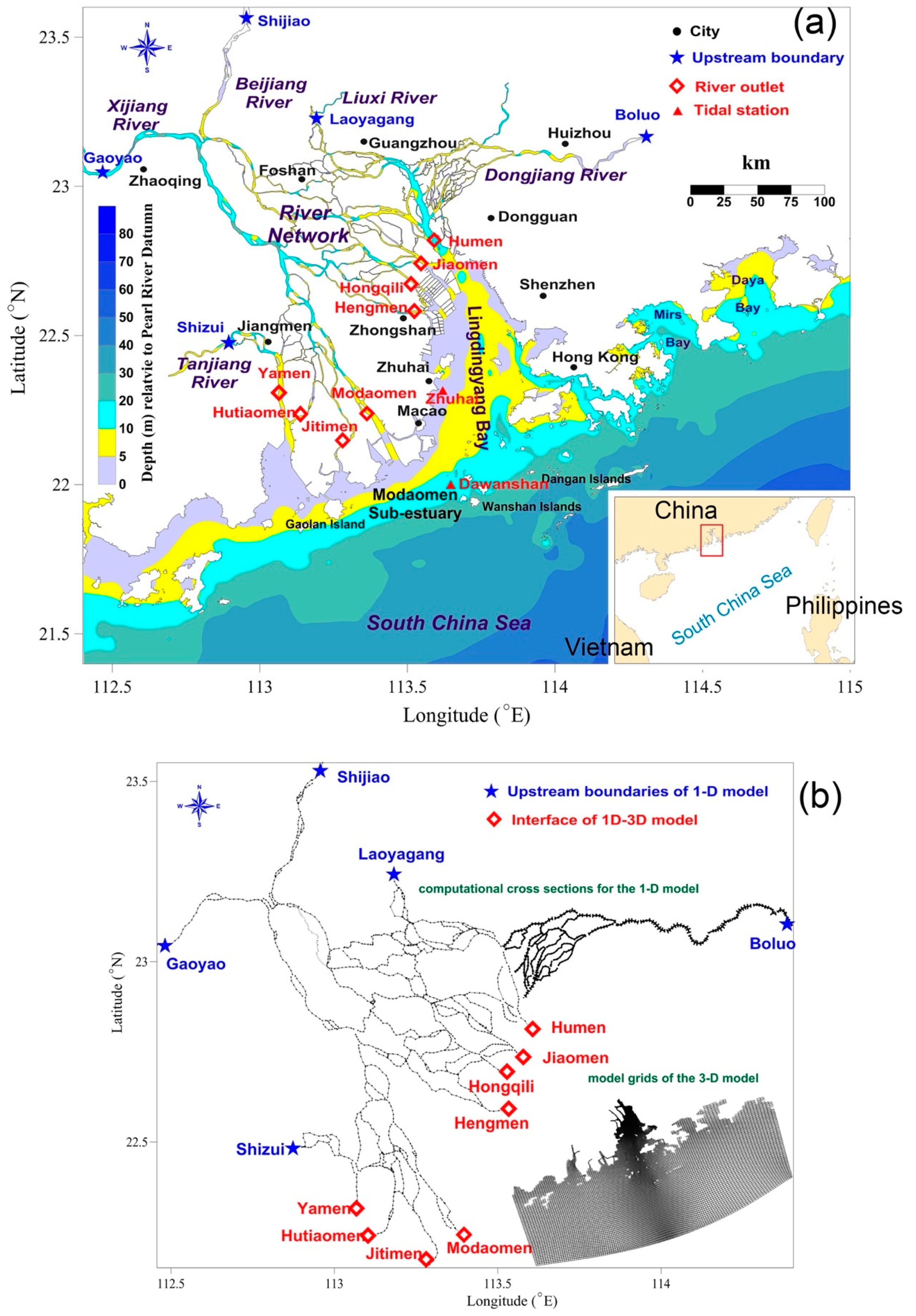
The PRE is closely connected with the upstream Pearl River network and these two areas frequently interact with each other. The hydrodynamic processes in the PRE are significantly affected by the large freshwater inputs from the river network. In order to better reflect the interaction between the river network and the estuary, it is necessary to fully consider the dynamic changes of the discharge across the eight river outlets (Figure 1a). However, the observational discharge data during the river outlets were absent for most of the time including our simulation period (2006). Alternatively, we used a one-dimensional (1-D) and a three-dimensional (3-D) coupled hydrodynamic model in this study to properly account for the interactive impacts of the river network and estuary on the hydrodynamics in the PRE. To simulate the water transportation in the river network, the Saint-Venant equations of mass and momentum conservation were solved by the Preissmann implicit scheme in the 1-D model. The Estuaries and Coastal Model with Sediment Module (ECOMSED) 3-D hydrodynamic model [31], which has been successfully applied to simulate transportation and circulation in the PRE [32,33], was used in this study. The model solves the Navier–Stokes equations for a water body with a free surface, under Boussinesq and hydrostatic approximations. The Smagorinsky-type formula and Mellor–Yamada level 2.5 turbulent closure scheme is used in the model [34]. The 1-D and the 3-D models were run in parallel (two-way online coupling) and they exchange model quantities across the coupling interface. As connections between the river and estuary, the eight river outlets in the PRE are the boundaries and interfaces for both models, which consider boundary conditions such as water discharge and water level exchange. At each computational time step, the 3-D model utilizes the simulated river discharge from the 1-D model as the river boundary forcing and in the meantime, also provides the simulated water levels to the 1-D model as the latter’s downstream boundary forcing for the next time step. A more detailed description of the methodology and implementation of the coupled hydrodynamic model is given in Hu and Li [1]. The 1D–3D coupled model has been validated using the observed water levels and/or river discharges at the eight outlets [1], and has been applied to study the water–nutrients–sediment budgets [1,32], the oxygen budget [30,33], and the nutrient fluxes between the sediment and overlying waters in the PRE [35].
The configurations of the hydrodynamic model are as follows. For the 1-D hydrodynamic model, five upper boundaries (i.e., Gaoyao, Shijiao, Boluo, Laoyagang, and Shizui; Figure 1b) were specified using hourly observed river discharge (the first three stations) or water level (the last two stations) derived from hydrologic stations located at the tributaries of the Pearl River; the lower boundaries (i.e., eight river outlets; Figure 1b) used the simulated water levels calculated from the 3-D model. The time step of the 1-D model was 5 s. For the 3-D model, the model domain extended from 112.5° E in the west to 115.5° E in the east. The southern part reached the 75 m contour line in the South China Sea (Figure 1b). The model had 183 × 186 grid cells with sizes varying from approximately 400 m inside the estuary to nearly 4000 m in the shelf area, and had 16 vertical sigma layers with a refined resolution at the surface and bottom layers. The water discharges of the eight river outlets used for the 3-D hydrodynamic simulation were calculated from the 1-D model at each time step. At the open boundaries, the tidal level was prescribed by the Oregon State University Tidal Data Inversion software (OTIS). The physical dynamics in the PRE are also affected by the South China Sea circulation [36]. Hence, the offshore non-tidal sea level was calculated according to Csanady [37] and imposed onto the western, eastern, and southern open boundary tidal forcing. The temperature and salinity of the open boundaries were obtained from the Simple Ocean Data Assimilation (SODA) package. Atmospheric data including wind speed, wind direction, shortwave radiation, air temperature, relative humidity, and barometric pressure were acquired from the ERA-Interim reanalysis data with a 6-h temporal resolution.
2.1.2. Water Quality Model
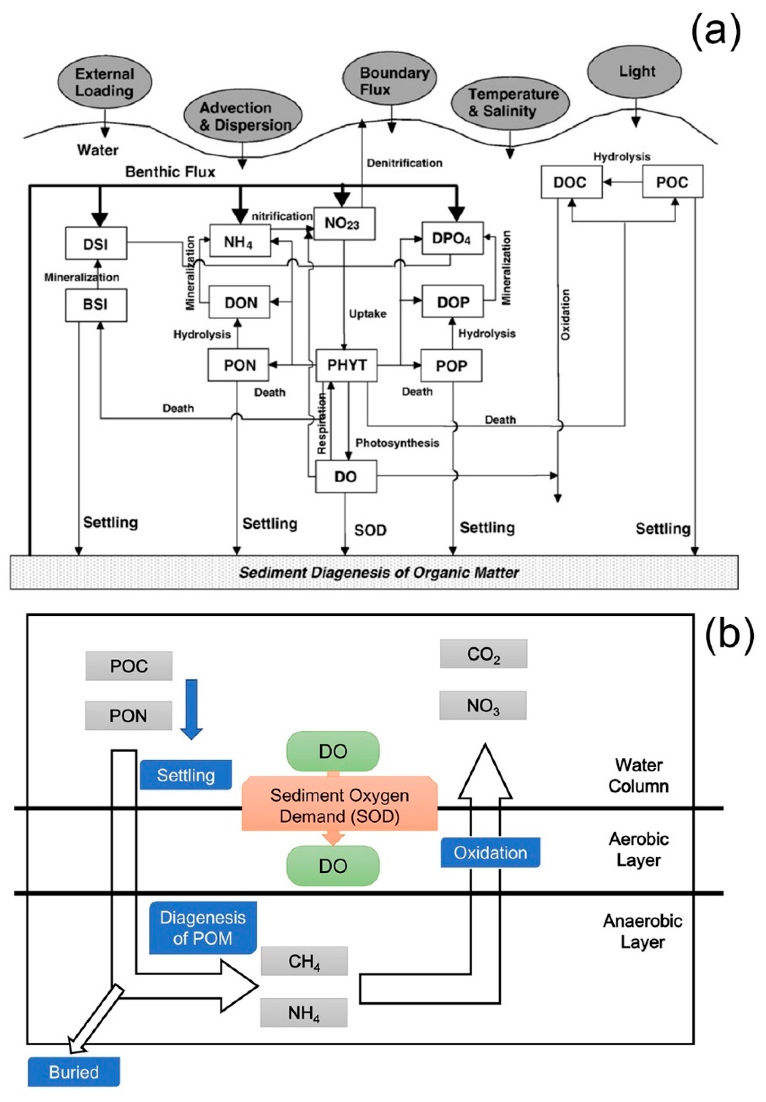
The water quality model was based on the Row Column Aesop (RCA) model, which is a water column and sediment biogeochemical model developed by HydroQual [38]. In the water column biogeochemical model, there are 26 state variables for six interactive matter cycle systems, namely, nitrogen, phosphorus, phytoplankton, silica, organic carbon, and DO. The RCA formulates mass balance equations for each state variable. For DO, the sources and sinks in the water column in the model are nitrification, algal photosynthesis and respiration, oxidation of dissolved organic carbon, and air-sea reaeration at the sea surface. The governing equation of DO in water can be expressed as follows:
where x and y represent the horizontal coordinates; z represents the vertical coordinate; u, v, and w (m s−1) represent the velocity components in the x, y, and z coordinates, respectively; and Ex, Ey, and Ez (m s−2) represent the dispersion coefficients. All of the velocity components and dispersion coefficients are computed by the hydrodynamic model. In addition, the term S represents the source/sink processes of DO; REA represents the air–sea oxygen exchange (mg O2 L−1 day−1); PHOT represents the production rate of DO by photosynthesis (mg O2 L−1 day−1); WCR (water column respiration) is the DO consumption rate in the water column (mg O2 L−1 day−1), which combines all of the biogeochemical DO depletion processes including respiration, nitrification, and oxidation; SOD represents the sediment oxygen demand (mg O2 L−1 day−1) at the water–sediment interface. A detailed description of each DO source/sink process kinetic equation in the water column can be found in Wang et al. [33].
S = REA + PHOT + WCR +SOD
As shown in Figure 2b, after particulate organic matter settles on the sediment, the diagenesis process in the anaerobic layer converts part of the particulate organic matter to dissolved matter (such as methane and ammonium). This dissolved matter will be oxidized in the aerobic layer and then transported to the water and sediment interface. The extent of the DO flux (mg O2 L−1 day−1) at the interface of water and sediment is defined as SOD (Equation (3)). At each time step, the water quality module calculates the fluxes of the particulate organic matters to the sediment module. Then, the sediment module calculates the SOD returned to the water quality module as one of the source/sink terms of DO in Equation (1). A more detailed description of the sediment kinetic equations can be found in Brady et al. [39] and Wang et al. [30].
Here, DOwater and DOsed represent the DO concentrations in the bottom layer of the water and sediment aerobic layers; H represents the thickness of the sediment aerobic layer; and Dc represents the transfer coefficient between the overlying water and sediment, which is a negative, representing the SOD is a sink to bottom water DO.
The simulation period for the water quality model was the same as the hydrodynamic model. The river boundary conditions at eight river outlets were set using the 2006 observed water quality data (such as ammonium, nitrate, phosphate, chlorophyll, and DO) collected by the State Oceanic Administration [40]. The organic matter concentrations were adopted from Ni et al. [41] and Liu et al. [35]. Monthly mean observation data (including ammonia, nitrite, nitrate, phosphate, and DO) from the State Oceanic Administration, reported in Zhang and Li [42], were specified as the open sea boundary. The point source loadings were obtained from reports by the local environmental protection agency. The primary water quality parameter setting was derived from previous research in the PRE [43] to ensure that the parameter values were within the accepted ranges (see Table A2 in Wang et al. [30]).
2.2. Model Experiments
The hydrodynamic model was run from 1 November 2005 to 31 May 2006, to ensure adequate time to finish spin up. The initial conditions for the water quality variables were derived from a spin-up simulation started five months before the simulation period. The water quality model was run offline using the same model grid of the ECOMSED model. The results of the hydrodynamic model from June to August were used as forcing for the water quality model. The realistic river discharge and wind forcing were used to force the base case simulation. In addition, several sensitivity experiments, as shown in Table 1, were conducted to evaluate the effect of main physical forcing (i.e., river discharge, wind, tide) on hypoxia in the PRE.
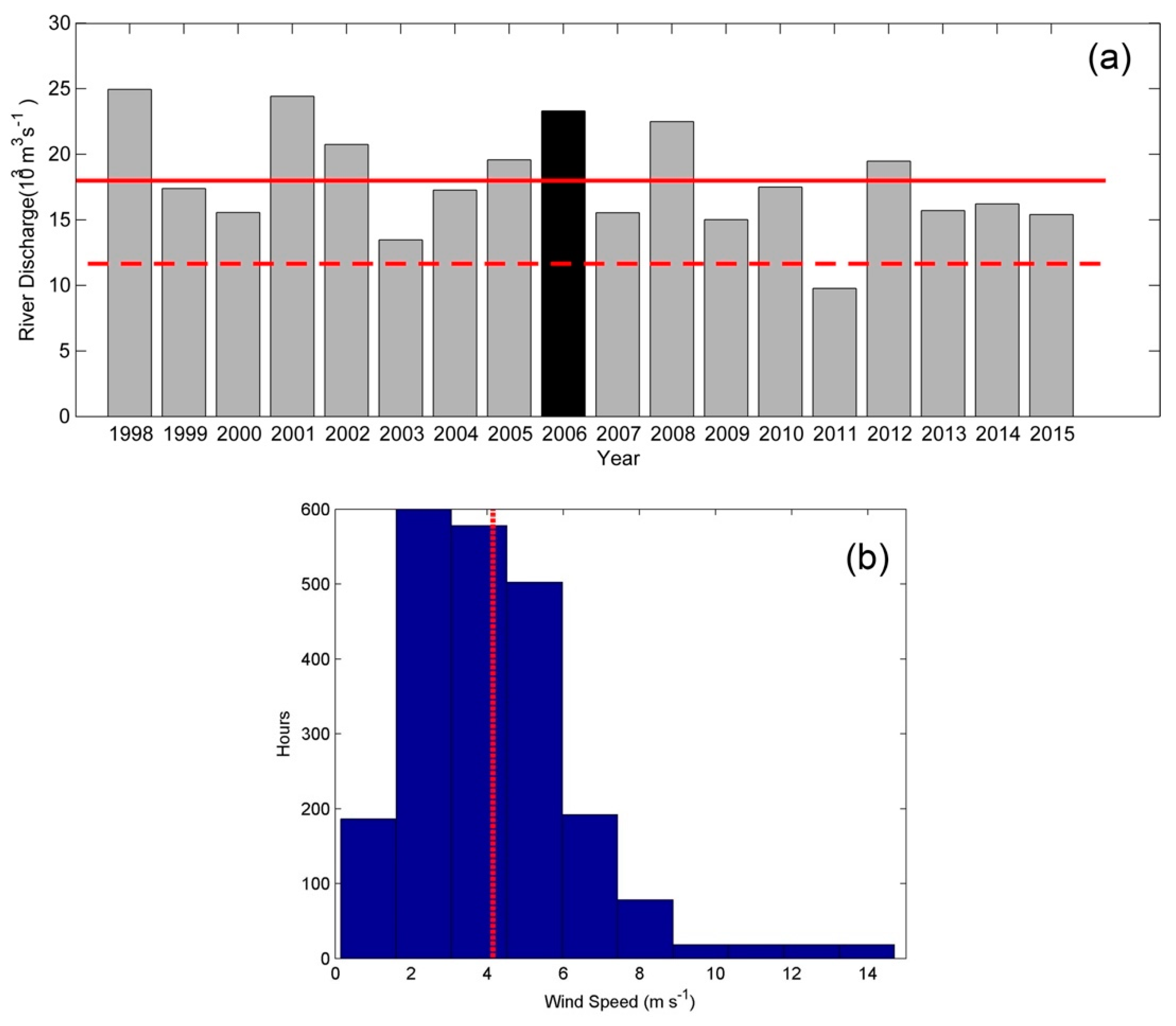
With respect to the river discharge, the annual values in the summers of 1998~2015 are shown in Figure 3a. The averaged summer river discharge was approximately 18,000 m3 s−1. The simulation with realistic forcing in 2006 was set as the base model run and is referred to as the wet year scenario. The averaged summer river discharge was approximately equivalent to 77% of the river discharge in 2006. Therefore, the RivMid model run with a river discharge at 75% of the base case level represented the moderate year scenario. The RivLow model run, representing the dry year scenario, had a river discharge at 50% of the base case, which was approximately within the 5% percentile of the 18-year river discharge range. For the riverine inputs of nutrients, DO, and POC, the concentrations were kept unchanged and the loads changed correspondingly to the river discharge for all of the river runs. Setting the nutrient concentrations unchanged is close to the reality where concentrations do not greatly change with river discharge [30].
The Pearl River basin is mainly controlled by the East Asian monsoon with a prevailing southwestern wind in the summer season. In the summer of 2006, the average wind magnitude was 4.05 m s−1 based on the statistical analysis (Figure 3b). The average wind run was conducted by forcing the model with a constant 4 m s−1 southwestern wind (WindConst case) to remove the variations in wind speed and direction. Although not realistic, this scenario, in comparison with the base run, helped explore the effect of real dynamic wind perturbation on hypoxia. To evaluate the effect of wind speed on hypoxia, the low wind scenario (WindLow case) was performed, which was forced by halving the wind speed of the realistic wind forcing of 2006. The wind speed of the strong wind scenario (WindHigh case) was set by doubling the wind speed of the base case. Although the wind speed value for the WindHigh case was relatively high for the summer average, strong wind events occasionally occurred during summer in the PRE. This case was conducted to explore the changes in DO under a strong wind situation.
Tides are an important source of energy for turbulence and mixing in estuaries, and they play a crucial role in the movement of dissolved and particulate matter by creating periodical variations in physical and chemical properties. First, we compared the DO characteristics and regulation mechanism during the neap tide and spring tide periods. Then, a run without tide forcing (no-tide case) was conducted to evaluate the effect of tides on hypoxia.
In order to evaluate the effects of different external forcing on the hypoxia quantitatively, five indicators were used in this study. The hypoxic frequency (HF) quantifies how often a waterbody experiences hypoxic conditions during summer (June–August), and is calculated following Luo et al. [19]:
where Ns is the total number of hours during summer and Nh is the number of hours over which hypoxia occurs.
The extent of hypoxia in each model run was quantified by the expected hypoxic area (HA), hypoxic volume (HV), and averaged water thickness of hypoxia (WTH):
where and are the area and volume of each model grid, respectively.
Stratification is an important factor for the development and maintenance of hypoxia in estuaries. The difference of density in the internal water body is the main reason for the formation of a stratified structure. In this study, the Brunt–Väisälä buoyancy frequency (BF) was calculated to quantify the strength of stratification:
where g is the acceleration of gravity; ρ is the potential density; and z is the vertical coordinate. Based on this definition, a greater BF corresponded to stronger water stratification.
3. Results
3.1. Model Validation
The hydrodynamic model was validated using the observed water level, salinity, and temperature. The water level data were obtained from eight tidal gauge stations as shown in Figure 1. Six of the stations were located in the river outlets, and the other two were located in the estuary. To quantitatively evaluate the model performance, the bias, root mean square error (RMSE), and correlation coefficient (Corr) were calculated as follows:
where N is the total number of observations; Simui and Obsi represent the simulated and the observed value of each state variable, respectively; Cov is the covariance; and σSimu and σObs represent the standard deviation of the simulation and observation, respectively.
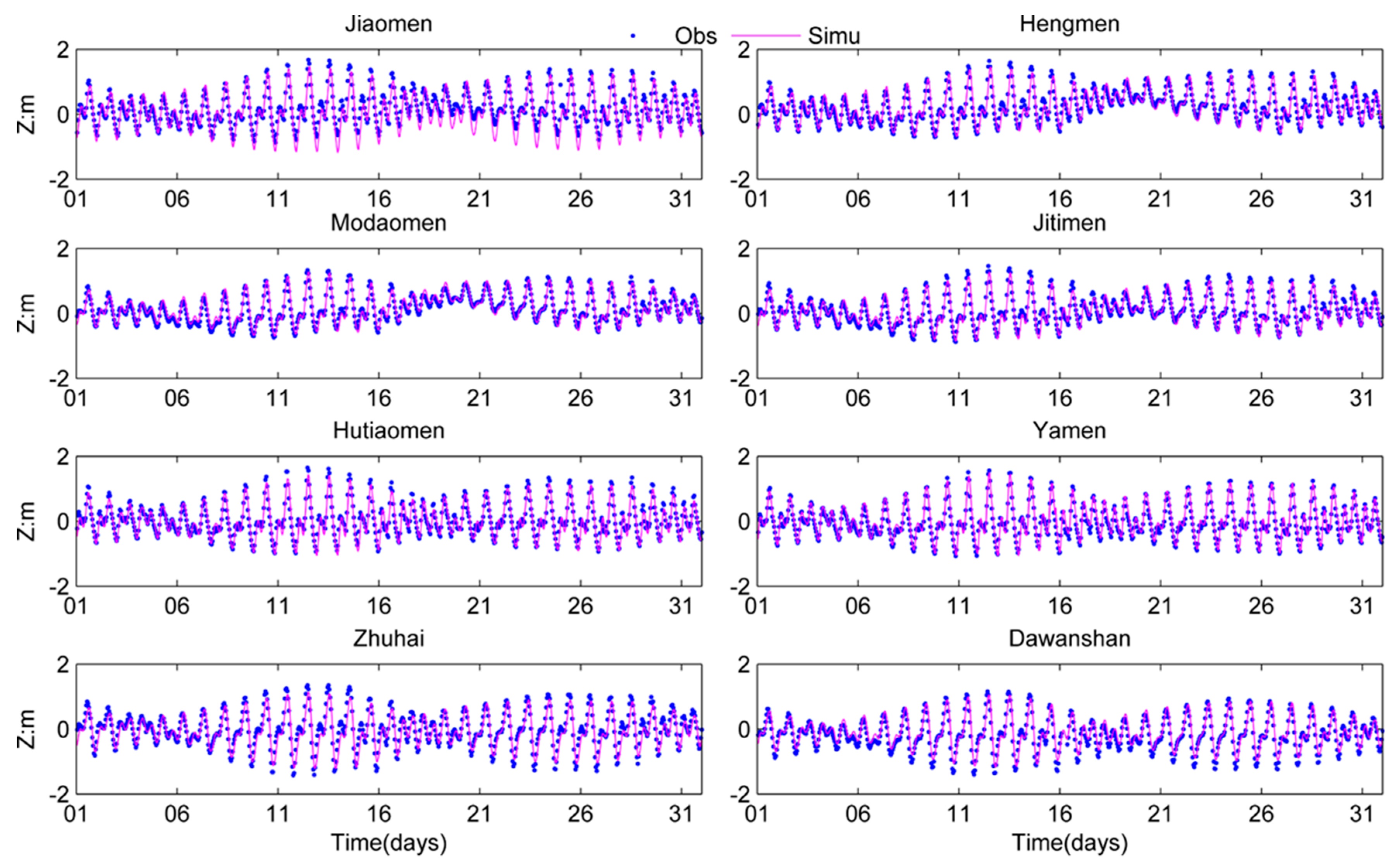
Figure 4 shows the comparisons between the simulated and the observed water level. At all eight stations, the biases of the water level were less than 12 cm when compared with the observations (Table 2). The biases of the water level were relatively low when compared with the water level variation ranges of these water level stations (~±1.6 m). At the east river outlets (Jiaomen and Hengmen) and estuarine stations (Zhuhai and Dawanshan), the RMSEs of these four stations were 20–25 cm. At the west outlets (Modaomen, Jitimen, Hutiaomen, and Yamen), the model performed well with the RMSEs ranging from 13–17 cm. The simulated water levels were closely consistent with the observations, and the correlation coefficients were greater than 0.91. The observation data for salinity and temperature were obtained from a summer cruise in 2006 organized by the South China Sea Branch of the State Oceanic Administration [44]. The samples were collected in the PRE and its adjacent area from 18 July to 21 August 2006. Here, point-to-point comparisons have been performed with time matching between the simulation and observation (Figure 5). Due to the high river discharge in summer, the Pearl River plume was distributed on the surface of the PRE (Figure 5a,b). The western extension of the plume could reach nearly 113° E along the western coast. At the bottom layer, high-salinity sea water occupied the offshore area (Figure 5c,d). The salinity increased from the river outlet area to the open sea area due to salt water intrusion, which caused a strong vertical gradient of salinity at the near-shore area. The model performed well in simulating the salinity distribution of the PRE and presented low bias (Table 2). The surface temperature of the PRE was approximately 27–30 °C due to the strong solar radiation in summer (Figure 5e,f). At the bottom layer, the temperature was relatively high near the outlet due to the shallow water of this area. As the water depth increased, the bottom temperature gradually decreased from the near-shore to offshore areas (Figure 5g,h). The model simulated the temperature pattern well with a bias of less than 0.1 °C and RMSE of approximately 1.08 °C (Table 2).
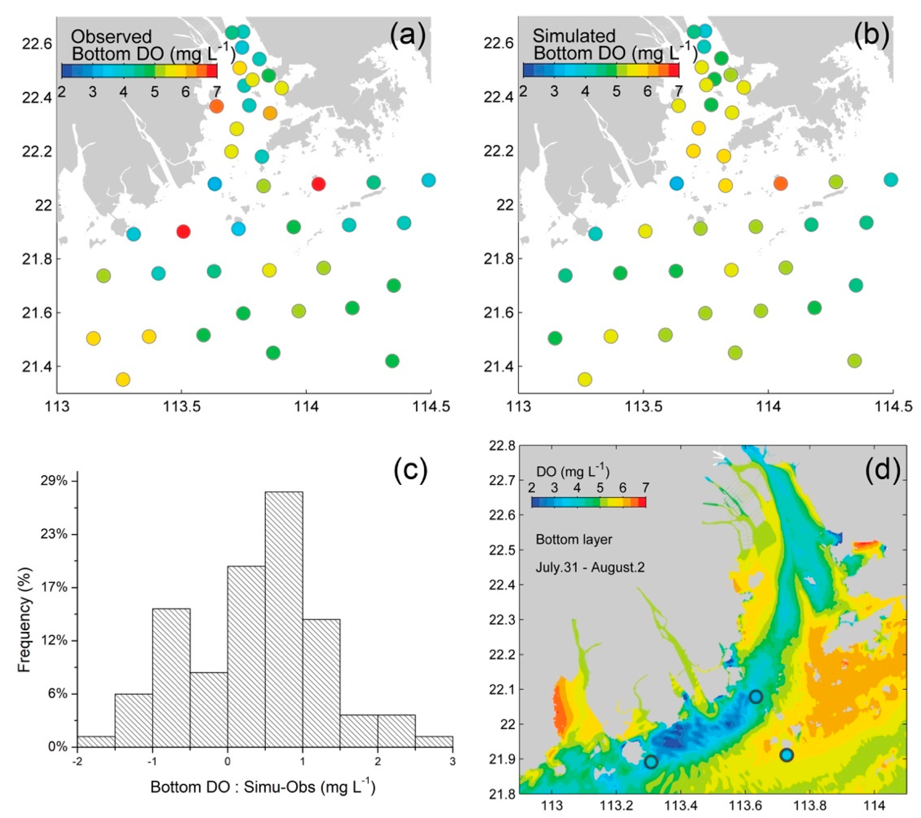
To validate the water quality model, the simulated DO concentration and DO-related key biogeochemical processes were compared with the observation data from sampling and the literature. The point-to-point comparisons of the bottom DO concentration between the observations and simulations were consistent (Figure 6a,b). More than 70% of the validation site had a bias within ±1 mg L−1 (Figure 6c). From late July to early August, the low DO area extended from the western part of the PRE (Figure 6d). Low DO values were observed in the Modaomen sub-estuary, and the simulation results also revealed these low DO zones. In addition, the particulate organic carbon (POC) and SOD, which are critical factors for DO consumption, ranged from 0.63 to 2.23 mg L−1 and −3.72 to −0.31 g m−2 day−1 in the simulation, respectively (Table 3). These ranges were close to the historical observed/estimated values in summer. The simulated average values of chlorophyll a and primary production were close to the corresponding observed values in the PRE. Overall, the validation indicated that our model was capable of reproducing the main hydrodynamic and water quality processes in the PRE, which allowed us to conduct research on the oxygen dynamics in the PRE.
3.2. Impact of River Discharge on Hypoxia
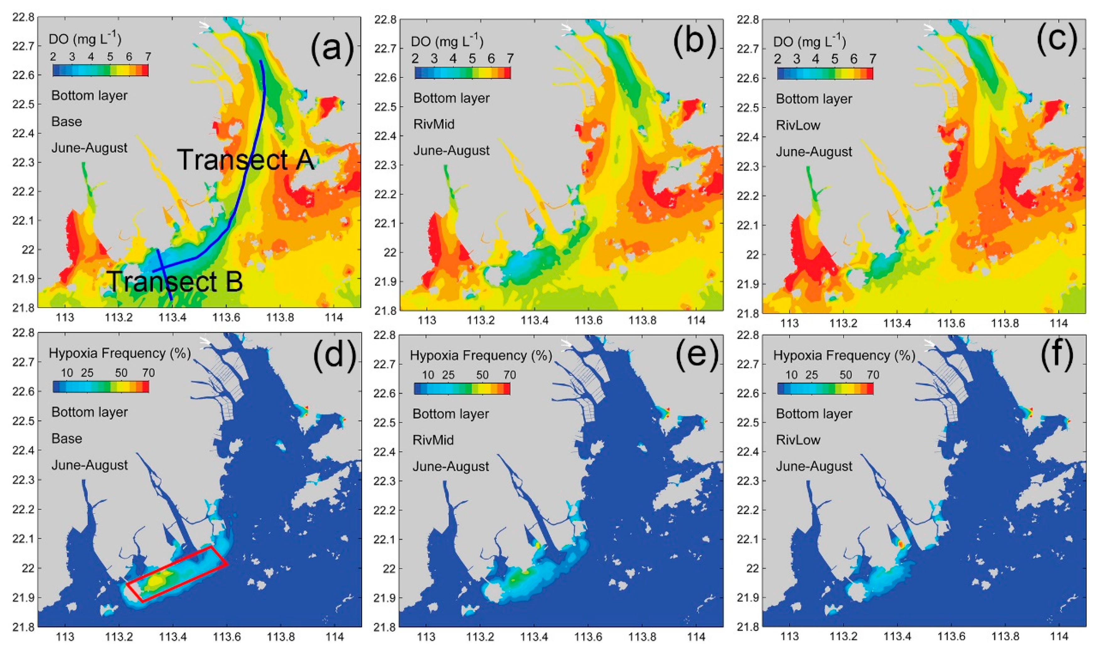
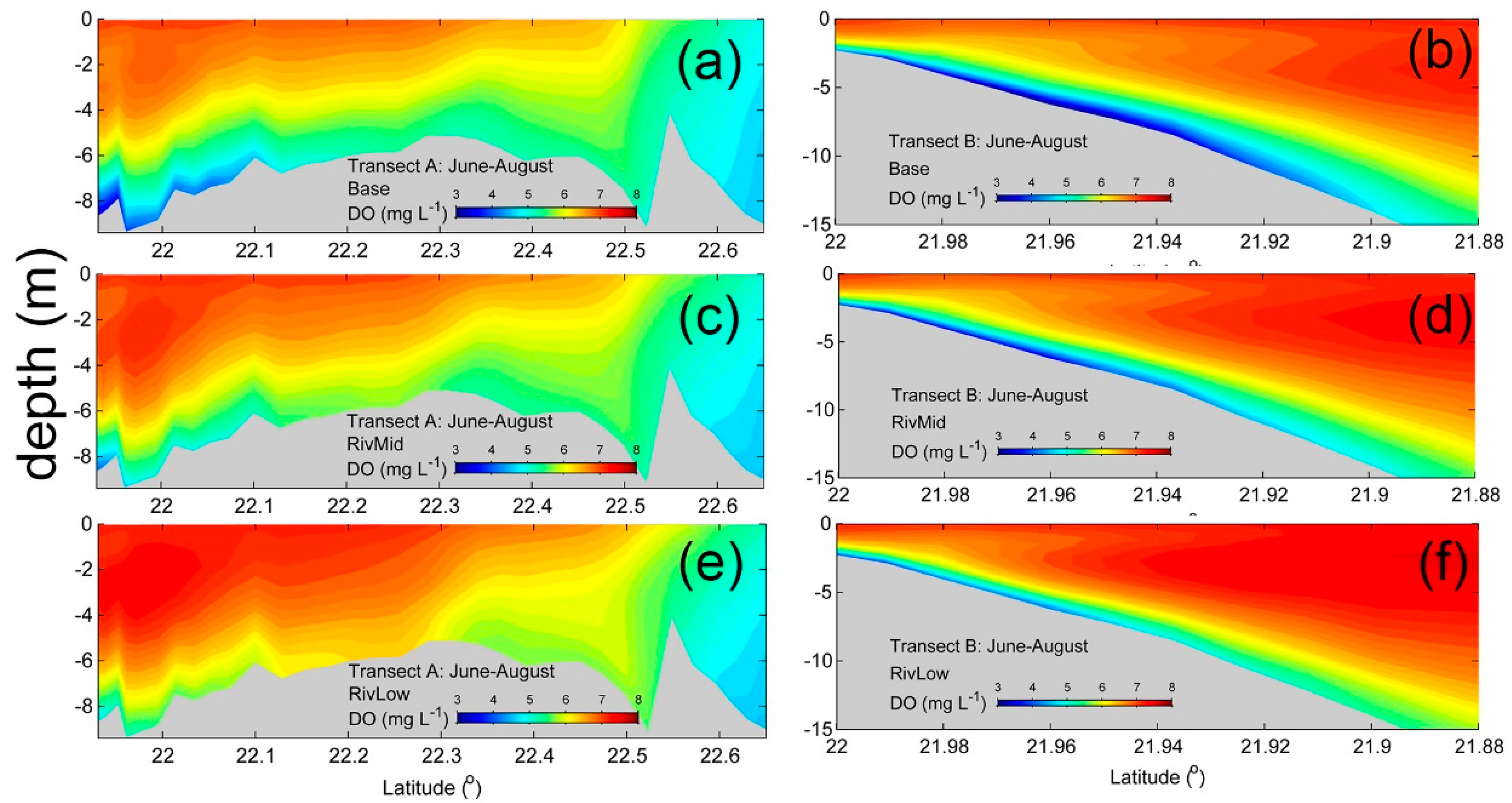
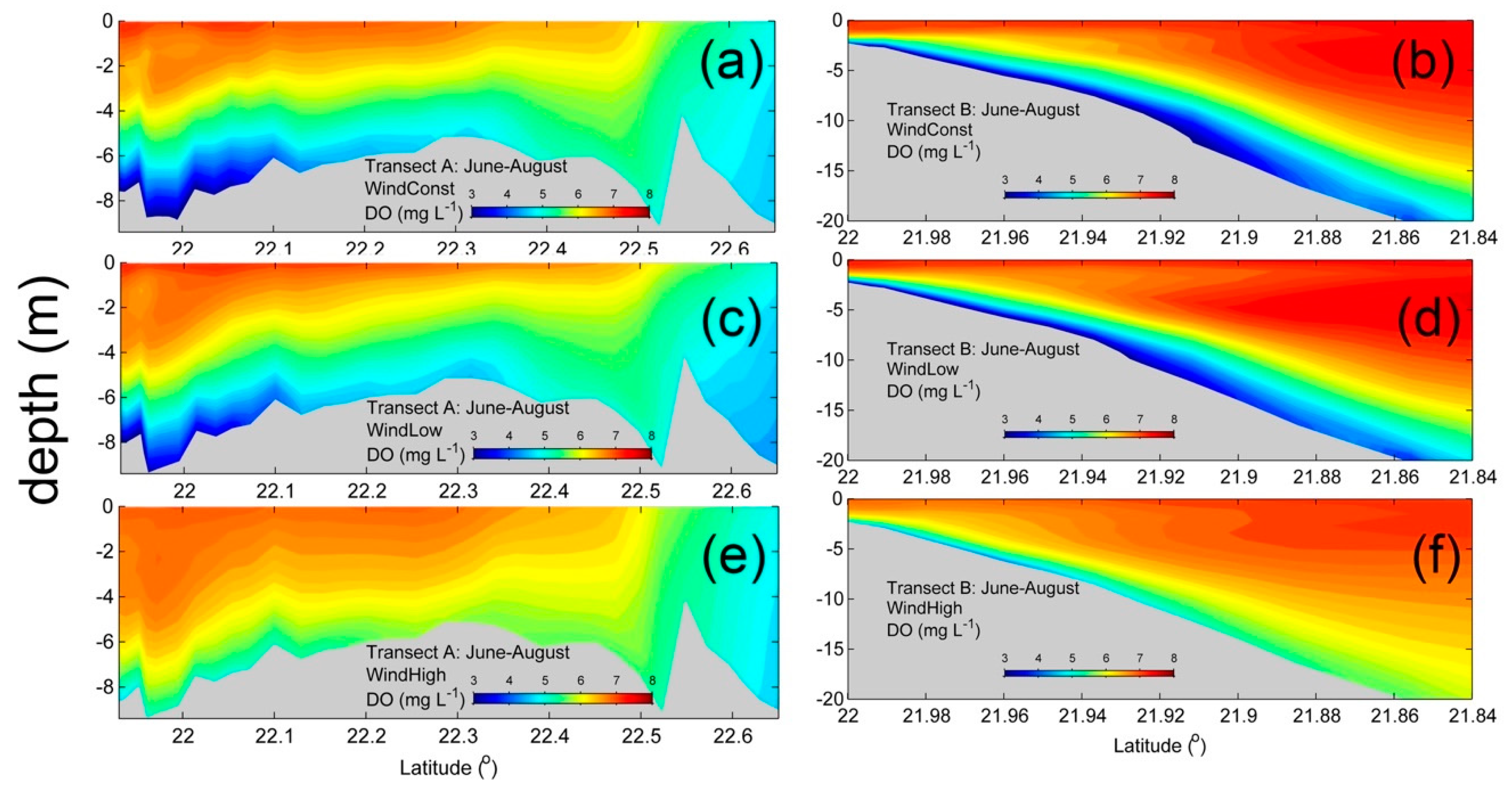
The summer bottom DO distribution in 2006 in the PRE is shown in Figure 7a (base case). The concentration of DO was relatively high in the middle part of the PRE. One of the low-DO zones was located near the Humen outlet, where the bottom DO concentration was lower than 5 mg L−1. The other low-DO zone was located from Gaolan Island to the outside of the Modaomen outlet and had an even lower bottom DO concentration of approximately 3 mg L−1. The hypoxia frequency was higher than 50% in the center of this hypoxic zone, which demonstrated that more than half of the summer season experienced hypoxia (Figure 7c). The low frequency HA (0% < HF < 50%) was approximately 113 km2, and the high frequency HA (HF ≥ 50%) was ~5 km2 (Table 4). This result indicates that hypoxia in the PRE was temporary. To further explore the vertical characteristics of DO, the DO profile of the two transects (transects A and B) is shown in Figure 8. A significant difference in the DO concentration was observed between the surface and the bottom layer at transect A (Figure 8a), with the bottom DO concentration lower than the surface DO concentration. A low-oxygen water mass was observed in the bottom layer at the lower part of the estuary (22° N). Along transect B, the DO was sufficient at the surface and gradually decreased with water depth. The low DO water mass was limited to a thin layer above the seabed (Figure 8b). The WTH was ~0.5 m (Table 4), which was equivalent to nearly 5~10% of the water column in the bottom layer that experienced hypoxia.
The bottom DO concentration and HF in the moderate year scenario (RivMid case), with a river discharge of 75% of the base discharge, are shown in Figure 7b,e. The high frequency and low frequency HAs were ~75 km2 and ~4 km2, respectively, which were decreased by 34% and 26%, respectively, when compared with the base run (Table 4). The averaged DO concentration increased in the vertical direction, and WTH decreased (Figure 8c,d). The HV was reduced by 45% when compared with the base case. In the dry year scenario (RivLow case), when the river discharge was halved, the bottom DO concentration further increased as the HA decreased (Figure 7c,f). Only a small hypoxic zone appeared west of the Modaomen outlet. Meanwhile, the difference in the DO concentration between the surface and bottom was small along transect A, and the DO concentration in the bottom layer further increased along transect B (Figure 8e,f). As a result, the HAs were reduced by 62% and 35% under low and high hypoxic frequency, thereby leading to reductions in the HV and WTH of 74% and 33%, respectively. Moreover, decreases in the river discharge reduced the hypoxic extent close to the near-shore shallow area.
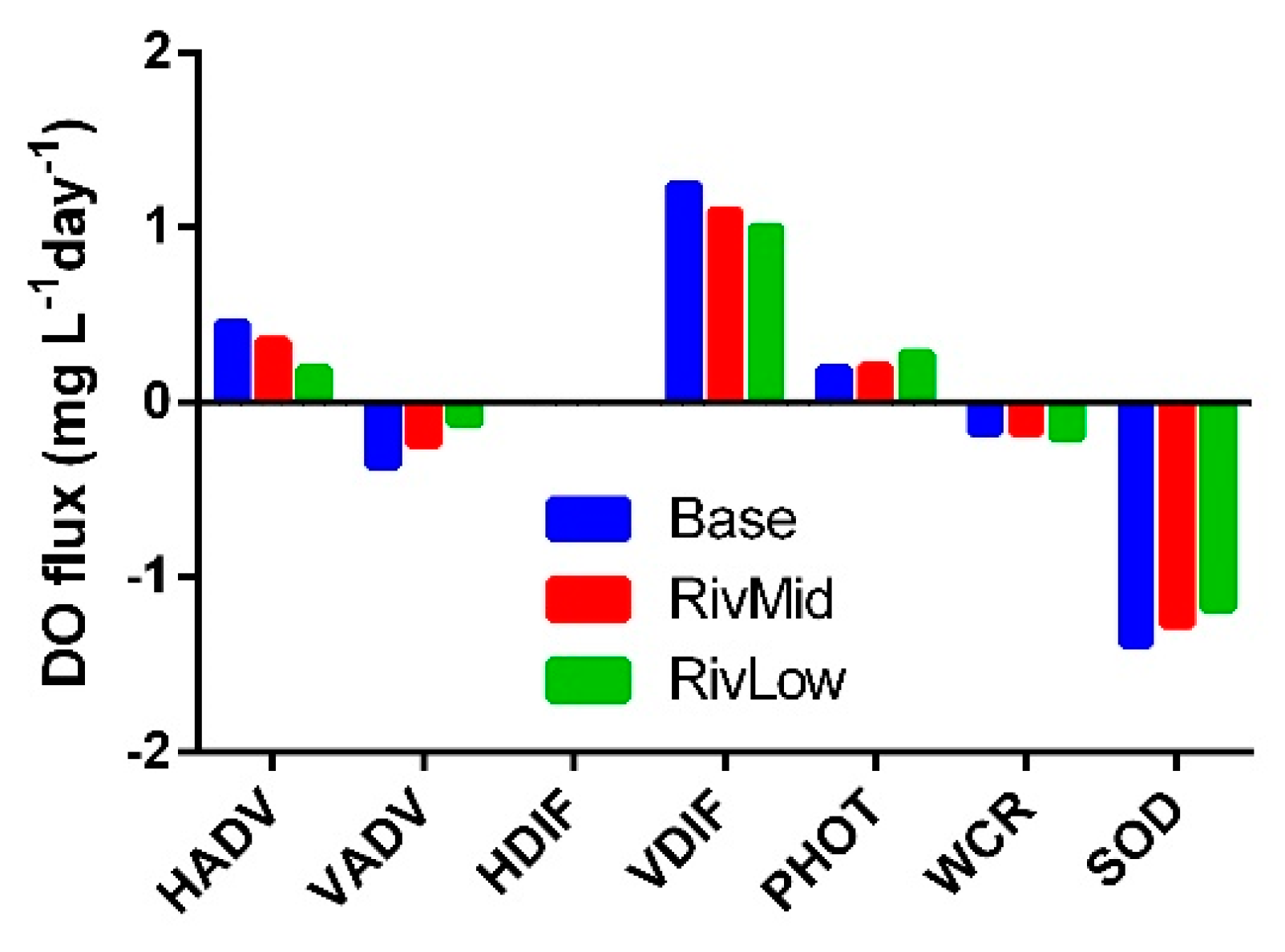
To identify the critical processes controlling DO dynamics, a diagnostic analysis of the DO budget was conducted with a fixed control volume in the center of the hypoxic zone in the Modaomen sub-estuary (Figure 7d). The thickness of the control volume was defined as 20% of the water column depth above the sediment. The oxygen budget calculated all the physical processes (including horizontal advection (HADV), vertical advection (VADV), horizontal diffusion (HDIF) and vertical diffusion (VDIF)), and biogeochemical processes (including PHOT, WCR and SOD). The DO budget showed that VDIF was the major process supplementing DO in the bottom water layer (Figure 9). The amount of HDIF was quite small when compared with VDIF. The DO replenishing by HADV was mainly from the river input from the Modaomen outlet, where the DO concentration was higher than that in the Modaomen hypoxic zone. The VADV was the sink of DO budget because vertical residual velocity was directed from the bottom layer to the middle layer, which reduced the oxygen from the control volume. The HADV and VADV nearly balanced each other. Among all of the biogeochemical processes, the SOD contributed the most to bottom DO depletion. Due to the high turbidity in the PRE, the DO production by photosynthesis was restricted and was approximately equivalent to the DO consumption by WCR.
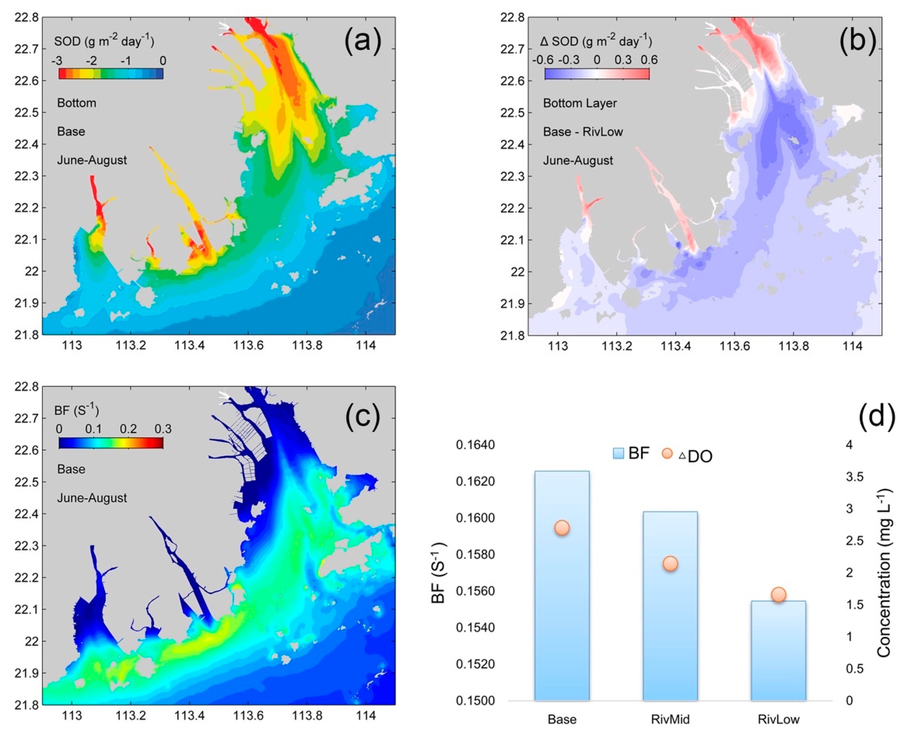
As shown in Figure 10a, the high-SOD zones were located near the river outlets, especially in the upper Lingdingyang Bay. In the RivLow case, less POC was delivered to the estuary and deposited on the sediment. As a result, the SOD decreased over the majority of the estuary when compared to the base model run (Figure 10b). In contrast, the SOD increased in areas near the river outlets because more organic matter from the river inputs was deposited near the outlets as the river discharge decreased. With respect to the VDIF (the most important process for DO supply), it is determined by both the water column stability and DO concentration gradient. Figure 10c shows the distribution of BF (the Brunt–Väisälä buoyancy frequency), which quantifies the strength of stratification, in the PRE during summer. The water was well mixed and weakly stratified near the river outlets inside the estuary. Strong stratification appeared in the Modaomen sub-estuary. Intense stratification inhibited the vertical water exchange, resulting in DO concentration differences between the surface and bottom layers that reached approximately 2.5 mg L−1 (Figure 10d). For the moderate and dry year scenarios, the BF value decreased, indicating that decreases in river discharge reduced water stratification and were beneficial to the exchange between the bottom oxygen-depleted water and the surface oxygen-rich water. However, the DO concentration gradient also declined with the river discharge due to the reduction in the SOD, which induced higher DO concentrations in the bottom layer. As a consequence, the DO concentration differences between the surface and bottom were 2.2 mg L−1 and 1.7 mg L−1 in the RivMid and RivLow cases, respectively. Therefore, the decrease of VDIF in the DO budget was mainly regulated by the DO concentration gradient when the river discharge decreased.
3.3. Impact of Wind on Hypoxia
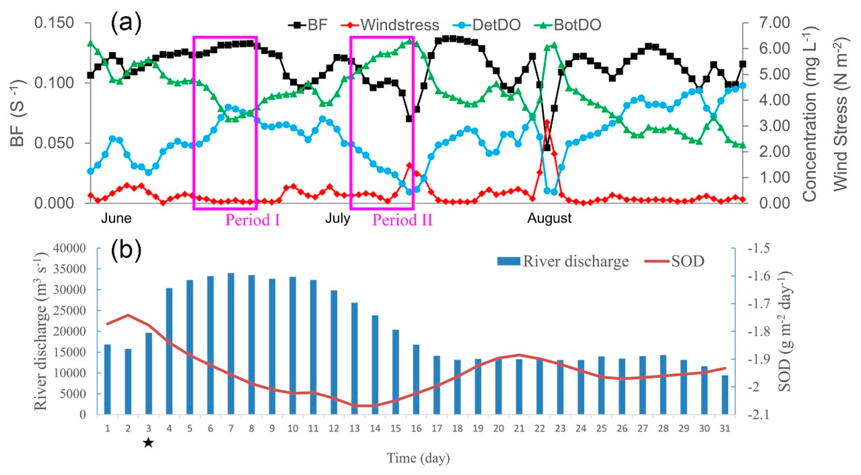
As above-mentioned, hypoxia in the PRE is episodic and transient, and hence needs to be investigated within a short time scale. Figure 11a shows the bottom DO concentration in the Modaomen hypoxic zone and the daily wind stress. The strength of wind stress had an impact on water mixing and stratification and affected the vertical exchange and bottom DO concentration. As shown in Figure 11a, the BF showed a negative relationship with wind stress (Corr = −0.76). During period I, the wind strength was weak, and the BF value rose consistently. The strong water stratification inhibited the vertical exchange of DO, thereby leading to a large DO difference between the surface and bottom layers. Meanwhile, the DO concentration of the bottom layer began to decrease and closely approached hypoxia. In contrast, during the strong wind period (period II), the BF significantly decreased. The weak stratification facilitated the vertical exchange of DO. As a result, the difference in the DO concentration between the surface and bottom layers continually decreased, and the bottom DO concentration increased to nearly 6 mg L−1. It should be noted that in early August, “Typhoon Prapiroon” (the No. 6 typhoon in 2006) landed near the PRE. This extremely strong wind event rapidly broke the water stratification and promoted vertical mixing that strongly impacted the vertical DO distribution. After the typhoon, the PRE experienced a long period of low winds. The BF quickly increased and remained high, indicating that the water stratification had reformed again. The DO gradient steadily increased due to stratification. As shown in Figure 11b, after the typhoon, the river discharge decreased and remained high for the first half of August, which led to a remarkable increase in terrestrial particulate organic matter load. The terrestrial particulate organic matter was transported outside the river outlet. Under the condition of high oxygen consumption and stable water columns, the bottom DO concentration in the Modaomen hypoxic zone continued to decline and remained hypoxic after mid-August.
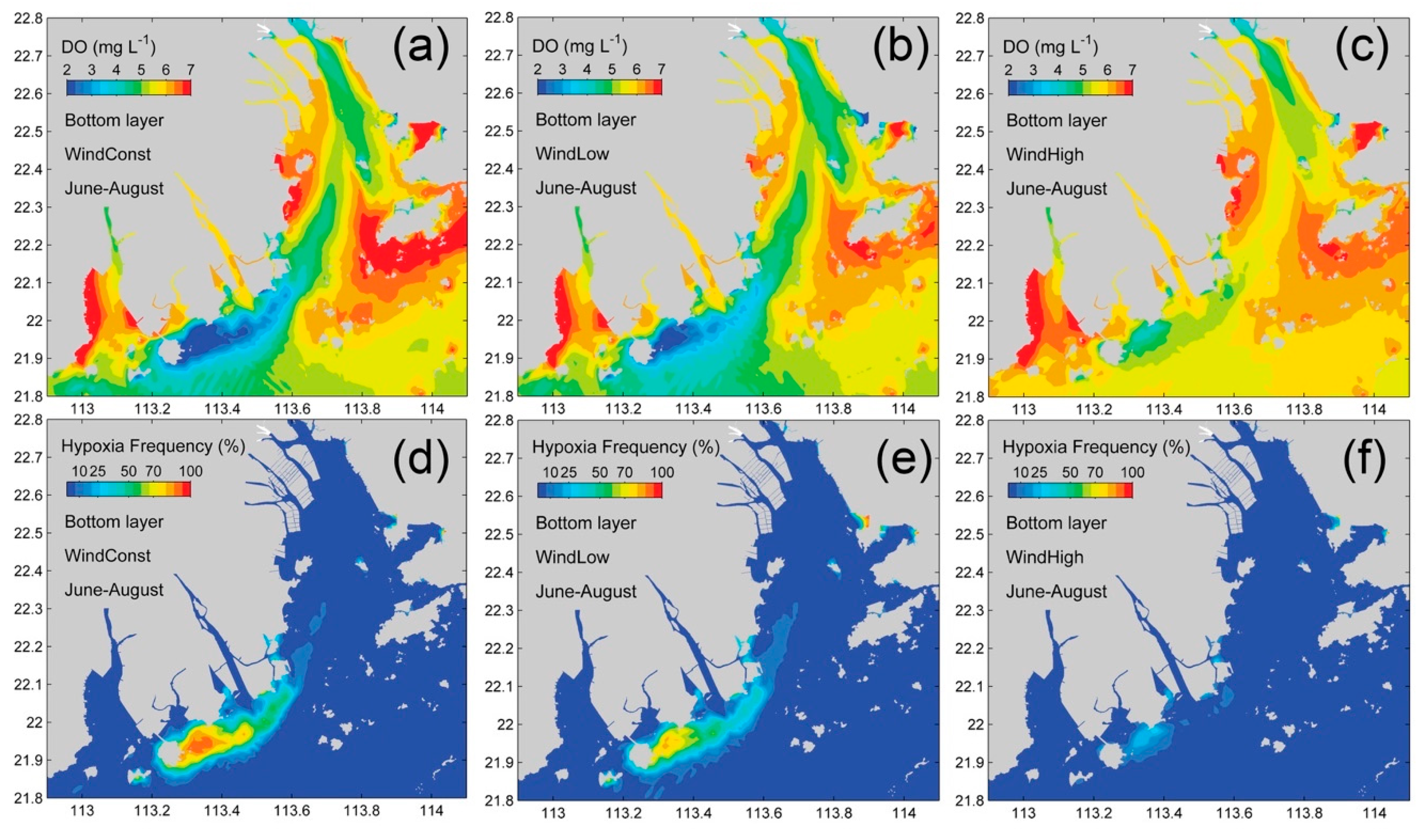
Given the wind effect demonstrated above, a scenario case with monthly averaged wind forcing (WindConst case) was conducted to explore the bottom DO dynamic without wind fluctuation. As shown in Figure 12a,d, the averaged concentration of DO was less than 3 mg L−1 in the Modaomen hypoxic zone, which was below the base case value. This hypoxic zone ranged from 113.3°E along the coast to 113.6°E. Hypoxia was more persistent in the WindConst case than in the base case, and the frequency of hypoxia in the center of this zone was higher than 70%. The high frequency HA was ~175 km2, which was nearly 29 times greater than the base run high frequency HA, and the low frequency HA was ~115 km2 (Table 4). There was a strong vertical DO gradient along both transects (Figure 13a,b). Along transect A, a low DO concentration was observed in water with a depth exceeding 5 m (DO < 5 mg L−1). In transect B, the depth of the hypoxic water exceeded 15 m. The WTH was higher than 0.9 m, which represented an increase of ~70% when compared to the base case. The HV was 0.27 km3, which was approximately three times larger than the base run hypoxia volume (Table 4).
Moreover, low wind (WindLow case) and strong wind (WindHigh case) scenarios were implemented to further explore the effect of wind strength on hypoxia. Under the low wind conditions, the bottom DO in the PRE was decreased when compared to that in the base case and hypoxic conditions remained in the Modaomen sub-estuary (Figure 12c,d). The area of low frequency hypoxia further extended to the middle of the PRE (22.3° N). The hypoxic areas had a significant increase when compared to the base case, with the low and high frequency hypoxic area increasing by approximately 31% and 15 times, respectively (Table 4). The DO distribution along both transects showed strong vertical gradient, with the DO-depleted bottom water isolated from the DO-rich surface water (Figure 13c,d). In contrast, under the strong wind scenario (WindHigh case), the bottom DO concentration significantly increased in the western part of Lingdingyang Bay and the Modaomen sub-estuary. In the western part of the Modaomen sub-estuary, the low frequency HA was ~44 km2, which represented a 61% reduction when compared to the realistic wind case (Figure 12c,f). In addition, the vertical DO concentration gradient further decreased. In the shallow area of the PRE (water depth < 5 m of transect A), the DO was vertically relatively well mixed. Along transect B, the DO concentration was more than 5 mg L−1 (Figure 13e,f), which presented an 18% reduction in the HV (Table 4).
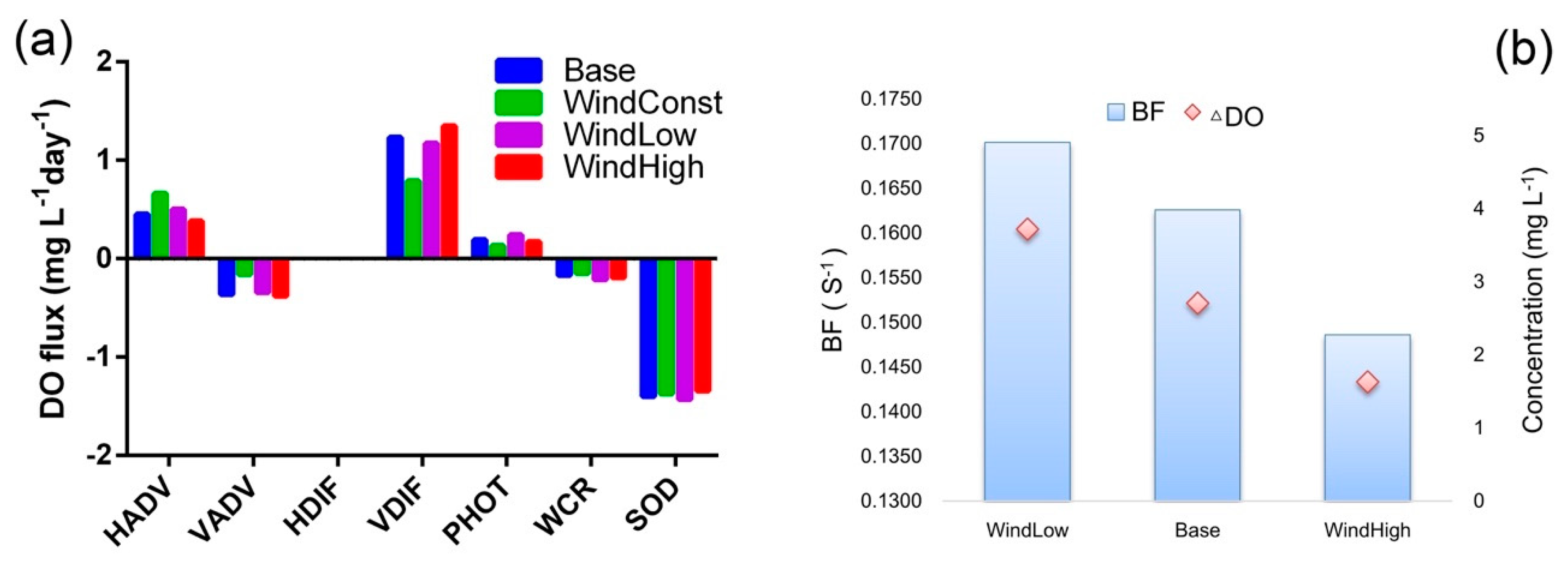
In the scenario with constant summer wind (WindConst case), the change in SOD was small in comparison to the base case (Figure 14a). Under average wind forcing conditions, the BF value was over 0.17 s−1, slightly higher than in the base case (Figure 14b). Strong water stratification inhibited vertical DO exchange. Consequently, the VDIF presented a significant decrease when compared to the base case. In the low wind scenario, the high BF indicated strong stratification, which induced a further decrease in VDIF (Figure 14a). The difference in the surface-bottom DO concentration was approximately 3.7 mg L−1 (Figure 14b). In contrast, in the high wind scenario, the strength of stratification weakened, and more DO replenished the bottom layer by vertical diffusion. As a consequence, the DO gradient across the water column was small (1.6 mg L−1). The results of the wind experiments demonstrated that the magnitude of wind speed regulated DO exchange by VDIF, which plays an important role in the development of hypoxia. Under strong wind conditions, the vertical water exchange was effective for supplying DO to the bottom layer.
3.4. Impact of Tides on Hypoxia
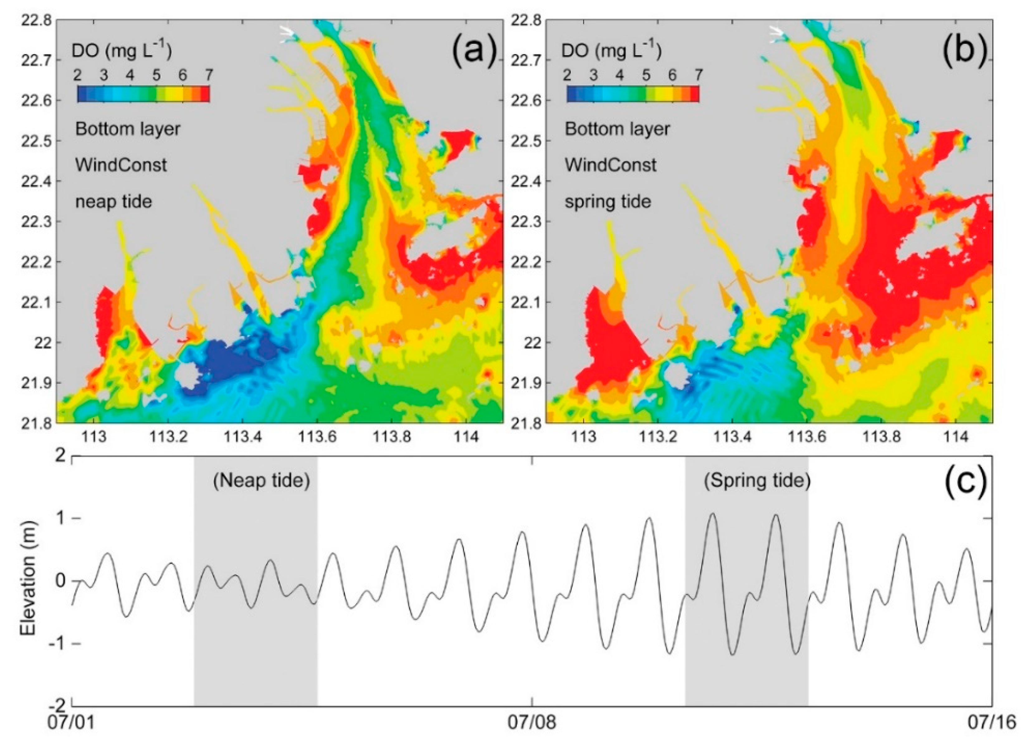
Figure 15 shows the bottom DO distribution during neap tide (3 July –4 July 2006) and spring tide (11 July–12July 2006) in the WindConst case, where the influence of the wind variability was removed. During neap tide, a large hypoxic zone with DO concentrations less than 2 mg L−1 developed outside the Modaomen outlet and extended to Gaolan Island. The west side of Lingdingyang Bay also experienced low-oxygen conditions (DO < 5 mg L−1). Nevertheless, during the spring tide in Lingdingyang Bay and the Modaomen sub-estuary, the bottom DO concentration significantly increased. The hypoxic zone outside the Modaomen outlet almost disappeared.
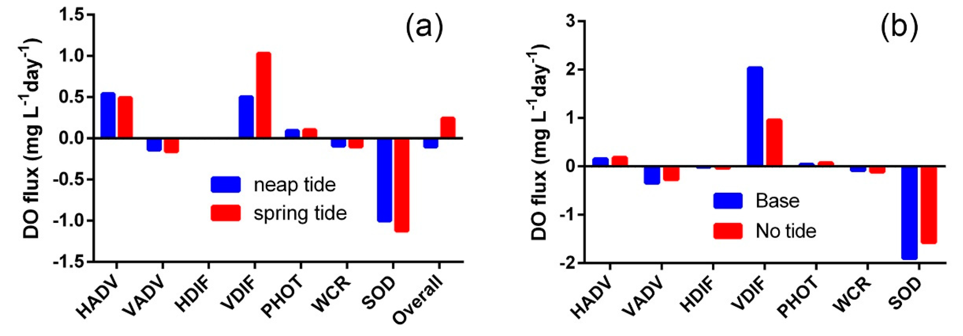
Figure 16a shows the DO budget during the neap tide and spring tide periods. Most of the physical and biogeochemical processes of the DO budget in the two tidal periods were roughly equal, except for VDIF. The VDIF at spring tide was almost twice as large as that at neap tide, with a slight reduction in the SOD. Due to the lack of DO supply, the net budget of DO in the bottom layer during the neap tide was −0.1 mg L−1 day−1. This finding indicated that the DO consumption rate was larger than the DO production rate, which induced a decrease in the DO concentration during neap tide. In contrast, during spring tide, strong tidal forcing led to a weak pycnocline and promoted VDIF. The net budget of DO was positive, which meant that, in the bottom layer, the DO supply exceeded the DO consumption. Consequently, with the increase in DO concentrations, hypoxia was relieved at spring tide.
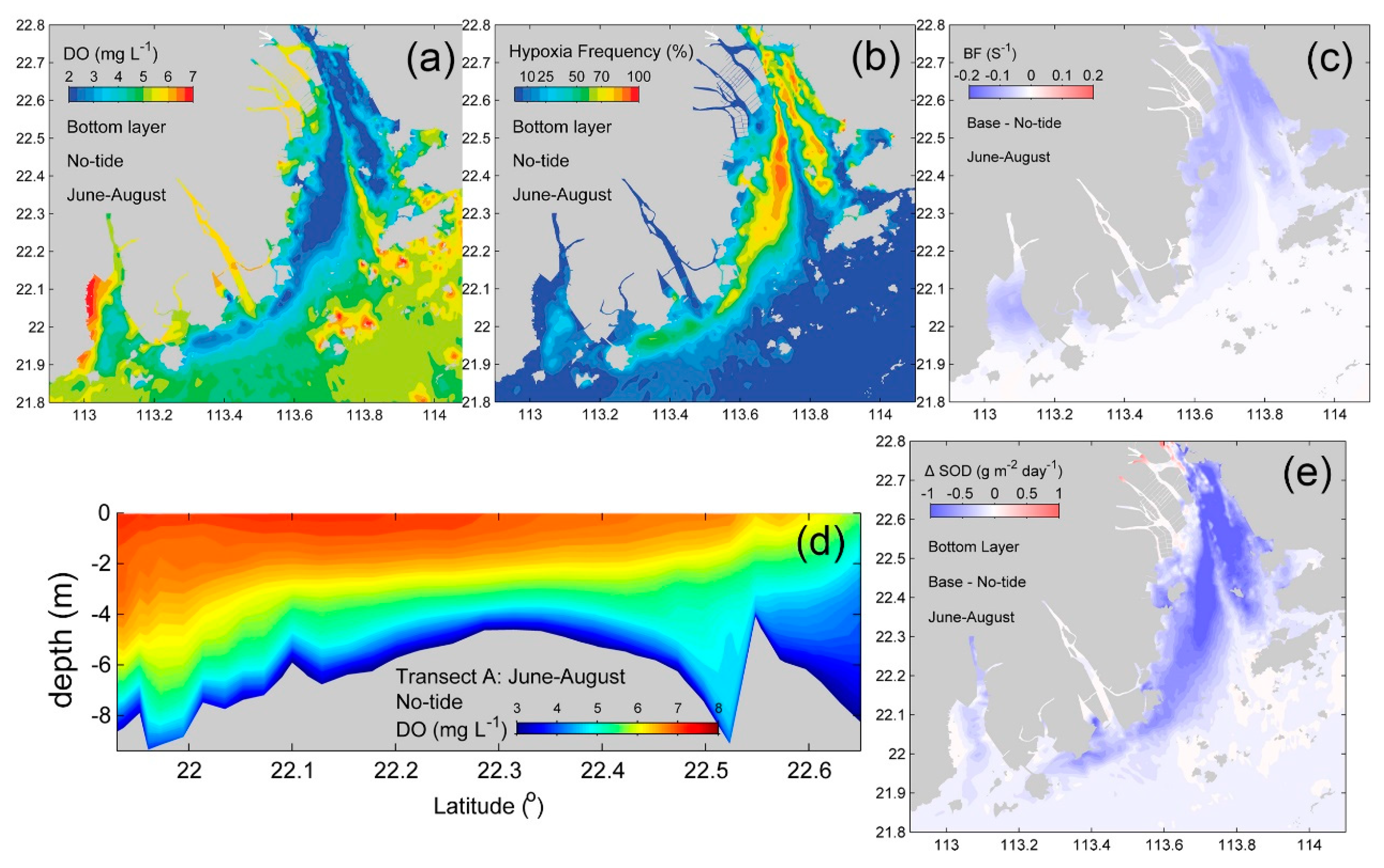
To further evaluate the effects of tides on hypoxia, a “no-tide” scenario was simulated. The model “no-tide” run had the same external force as the base model run, but the tidal forcing was excluded. As shown in Figure 17a, without tidal forcing, the DO concentration dramatically decreased. At the east and west shoals in the PRE, the averaged DO during the summer season was less than 2 mg L−1. The main hypoxic zones were located in Lingdingyang Bay (Figure 17b). The HA was more than 1100 km2, which represented a 110-fold increase when compared to the base case, and the HV was approximately 0.55 km3 (Table 4). The vertical gradient of DO was obvious along the PRE transects. The proportion of the low-oxygen water mass in the water column exhibited a downward trend from the outlet to the outer estuary (Figure 17d), which indicated that low DO accumulated inside the estuary, and the DO exchange between the inner and outer PRE was weak.
The budget showed that the amount of SOD in the no-tide case was smaller than that in the base case (Figure 16b). The current in Lingdingyang Bay had a southward flow due to the Pearl River runoff, and in the absence of tides, it was easier to transport terrestrial organic matter and nutrients out of Lingdingyang Bay, thereby leading to a reduction in SOD. Given the fact that the magnitude of PHOT and WCR were much lower than the SOD and that these two terms almost balanced each other, the changes in the nutrients’ effects on DO concentrations were neglected. Moreover, SOD was also regulated by the DO concentration gradient at the water–sediment interface according to Equation (3). Due to the lower bottom DO concentration in the no-tide case than in the base case, the flux of SOD was further inhibited. In addition, stratification significantly increased in Lingdingyang Bay due to the lack of tides (Figure 17c), which almost halved the amount of VDIF (Figure 16b). Due to the lack of DO supply, a persistent and large extent of hypoxia appeared in Lingdingyang Bay without tidal forcing.
4. Discussion
In this study, we conducted a suite of numerical experiments as well as a DO budget analysis to diagnose the response of hypoxia and its associated underlying mechanisms to external forcing such as river discharges, wind, and tidal forcing. The model results were generally consistent with previous studies [26,27] and also served as a complementary to those studies.
4.1. Effects of River Discharge
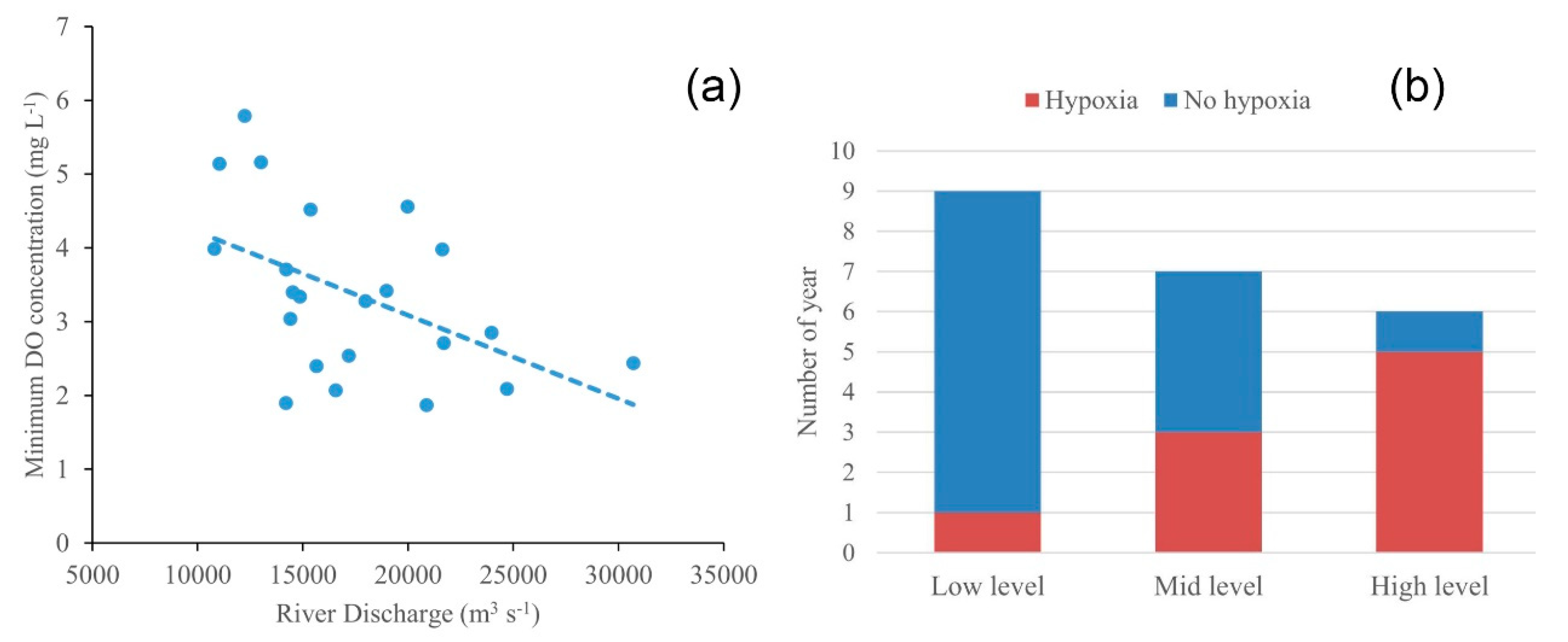
The model simulations confirmed significant effects of river discharge on hypoxia in the PRE where the hypoxia was largely alleviated by lower river discharge. This declining trend in the hypoxic extent with a decreasing river discharge has been reported in a previous study [26] and in other hypoxic systems, for example, the Northern Gulf of Mexico [16] and Changjiang Estuary [47]. In addition, we collected a suite of observations spanning 25 years, which were conducted by the South China Sea Branch of the State Oceanic Administration from 1982 to 2006. Despite the temporal and spatial scarcity, the observations demonstrated a negative correlation between the river discharges and the observed lowest DO concentrations in summer (June–September, Figure 18a). In addition, we categorized river discharge into three levels, and found an increasing probability of hypoxia with higher river discharge levels (Figure 18b). Hypoxia was observed in five of six years with high-level river discharges (>20,000 m3 s−1) while the proportion of years when the hypoxia occurred with mid-level river discharges (15,000~20,000 m3 s−1) was only 43%. Moreover, the hypoxia was rarely observed with low-level river discharges (<15,000 m3 s−1). However, it should be mentioned that the spatial distributions of these sampling sites varied a lot from year to year. In some years, there was only one cruise during the whole summertime. As such, the observations were insufficient to fully represent the real DO conditions, which highlights the necessity of more observations in the PRE.
The changes in DO concentrations and hypoxia under the different river discharges were associated with both stratification and river load. The importance of stratification for hypoxia has long been investigated [47]. With respect to the riverine loads, Wang et al. [30] investigated the response of hypoxia and oxygen dynamics in the PRE to variations of DO, nutrients, and POC inputs, and found that hypoxia was most sensitive to the riverine inputs of POC followed by DO and nutrients. This was in contrast to other hypoxic systems where the close relation between the nutrient load and hypoxia was observed [5,48]. Wang et al. [30] attributed the difference between the PRE and other hypoxic systems to the dominant roles of terrestrial POC in relation to the marine POC inputs. Using the same model as Wang et al. [30], we further support the statement based on DO budget analysis under different levels of river discharge (Figure 9). We showed that the magnitude of photosynthesis (PHOT) and water column respiration (WCR) as well as their relative changes in river runs were much smaller than that of the SOD. Therefore, the concurrent increase of terrestrial POC inputs with river discharges contributed to the deterioration of hypoxia, which would be valuable for hypoxia management in the PRE.
Although some recent studies based on observations have suggested that hypoxia in the PRE was more dependent on marine POC [24,49], this does not conflict with our study. The relative contributions of marine versus terrestrial POC to the SOD had significant spatio-temporal heterogeneity and was dependent on the river discharges in the PRE. Generally, in wet seasons (May–September) the terrestrial POC was more important in the upper region and west-shore area in the PRE [50,51], and gradually decreased seaward as the impact of river discharges weakened, which led to the high consumption of bottom DO in the west side of Lingdingyang Bay and the Modaomen sub-estuary. Furthermore, the low DO concentration near the Humen outlet was mainly affected by low DO river inputs due to the nitrification and terrestrial organic matter degradation in the upper reach of the PRE [52].
4.2. Effects of Wind
Wind-induced mixing is another key factor that controls stratification and hypoxia in the PRE. In this study, we performed a suite of numerical experiments with different wind stress, and found that higher wind stress tends to produce weaker hypoxia. Wang et al. [30,33] estimated that about 28% of oxygen replenished by re-aeration could penetrate to the bottom waters through the vertical diffusion, which highlighted the importance of reaeration for hypoxia in the PRE. Therefore, we can infer that the high wind stress inhibited the formation of hypoxia by facilitating the air–sea reaeration and penetration of DO through the vertical mixing. Therefore, wind stress can influence hypoxia not only through stratification, but also via the air–sea reaeration.
Furthermore, hypoxia in the PRE may also be affected by wind direction. We conducted an additional case with a southeasterly constant wind of 4 m/s to investigate the sensitivity of hypoxia to wind direction. The simulated hypoxic area for this case (shown in Figure S1 in the Supplementary Material) declined when compared to the Windconst case (with a constant southwesterly wind of 4 m/s), and the hypoxia was relatively closer to the shore. Specifically, the southeasterly (downwelling-favorable) wind drove the surface water onshore and the bottom water offshore at the near-shore area, which weakened the water column stratification and facilitated the supply of bottom DO. Our results demonstrated that in addition to wind speed, the change in wind direction also played a role in regulating the hypoxia in the PRE.
The wind forcing in the summer of the PRE was highly variable and the comparisons of the stratification against wind stress showed the effects of the short-time scales of winds on stratification and hypoxia (Figure 11). In order to understand the effects of these high-frequency variations in the wind stress on hypoxia, we compared the model results between WindConst and the base run, which suggest that the high-frequency variations in wind forcing is an important mechanism to restrain the stratification as well as the formation and maintenance of hypoxia in the PRE. This mechanism provided a complementary explanation to the tidal forcing for the intermittence of hypoxia in the PRE and has not been reported in other previous studies.
4.3. Effects of Tide
The influence of tidal forcing on the hypoxia in the PRE was also investigated in this study. Tides are a key factor in the occurrence of hypoxia, especially in shallow locations of the PRE. With tidal forcing, the bottom low-oxygen water caused by sediment consumption can be easily mixed with the upper water layers in shallow water. Analogous to the Changjiang Estuary where the hypoxic area is significantly larger when the tidal forcing is removed [53], the hypoxic volume in the PRE was about 7-fold larger without the tide. However, the hypoxia during neap tide in the Changjiang estuary is more severe than that without the tide. This is because during the neap tide, the Changjiang river plume extends further eastward, leading to much larger stratified areas relative to the case without tide forcing. In contrast, the tidal mixing outperformed river plume in the PRE and the hypoxia was more serve without tidal forcing than during the neap tide.
5. Conclusions
We used a hydrodynamic-biogeochemical model to examine the impacts of river discharge, winds and tides on hypoxia in the PRE and identify the key processes controlling the DO dynamics based on model sensitivity experiments. The results showed that summertime hypoxia was greatly affected by river discharge. A notable decrease in hypoxia was observed under low levels of river discharge primarily because of the reduction in riverine particulate organic carbon transported to the PRE, which led to reduced SOD and hypoxia. In addition, the water stratification strength also decreased as river discharge decreased, which facilitated the supply of bottom DO by intensified VDIF.
Highly variable winds, especially intermittent strong wind, were favorable for the replenishment of bottom DO, which inhibited the development of hypoxia in the PRE. The results from the wind sensitivity experiments showed that in the low wind scenario, both HA and HV were largely increased, and a bottom hypoxic zone extended from the Modaomen sub-estuary to the western shoal of Lingdingyang Bay. In contrast, hypoxia dramatically decreased in the high wind scenario. The DO budget indicated that wind regulated the bottom DO concentration mostly by VDIF and HADV, although it had a limited impact on the processes of DO consumption.
The DO concentration fluctuated periodically with the tides in the PRE. The results of the model experiment without tide forcing showed that severe hypoxia occurred in the shallow areas of the PRE. The DO budget indicated that tides regulated the oxygen concentration by affecting both supply and consumption of DO. Although enhanced tidal mixing promoted the VDIF and led to an increase in bottom DO concentrations, the higher DO gradient at the water–sediment interface led to intensified SOD.
Supplementary Materials
The following are available online at https://www.mdpi.com/2073-4441/11/10/2080/s1, Figure S1: Comparison of the simulated dissolved oxygen (DO) concentration (a,b) and hypoxia frequency (c,d) in the bottom layer between the WindConst case (with a constant southwesterly wind of 4 m/s) and SE-Wind case (with a constant southeasterly wind of 4 m/s).
Author Contributions
For this study, J.H. (Jia Huang) performed the model simulations and wrote the manuscript with contributions from all co-authors. B.W., Y.X., B.L., and D.L. assisted in establishing the model. B.W., J.H. (Jiatang Hu), and S.L. assisted to revise the manuscript. This work was supervised by J.H. (Jiatang Hu) and S.L. We certify that this paper consists of original, unpublished work that is not under consideration for publication elsewhere.
Funding
The research was supported by the National Natural Science Foundation of China (grant no. 41306105), the Public Science and Technology Research Funds Projects of Ocean (grant no. 201305019), the Science and Technology Planning Project of Guangdong Province, China (grant no. 2014A020217003), the Fundamental Research Funds for the Central Universities (grant no. 17lgzd20), and the Guangdong Natural Science Foundation (grant no. 2014A030313169).
Acknowledgments
The authors also thank the editor and all anonymous reviewers for their invaluable comments and constructive suggestions to significantly improve the quality of the manuscript.
Conflicts of Interest
The authors declare no conflicts of interest.
Appendix A

Table A1.
List of main acronyms and descriptions in this paper.
| Category | Acronym | Description |
|---|---|---|
| Related to water quality variables | DO | Dissolved Oxygen |
| POC | Particulate Organic Carbon | |
| Chl a | Chlorophyll a | |
| Related to the DO budget | REA | Re-aeration at the air–sea interface |
| PHOT | Photosynthesis | |
| WCR | Water Column Respiration | |
| SOD | Sediment Oxygen Demand | |
| HADV, VADV | Horizontal/Vertical Advection | |
| HDIF, VDIF | Horizontal/Vertical Diffusion | |
| Related to indicators for hypoxia and stratification | HF | Hypoxic Frequency |
| HA | Hypoxic Area | |
| HV | Hypoxic Volume | |
| WTH | averaged Water Thickness of Hypoxia | |
| BF | Brunt–Väisälä Buoyancy Frequency | |
| Related to model experiments | Base | Model run with realistic forcing |
| RivMid, RivLow | River discharge experiments runs | |
| WindConst, WindLow, WindHigh | Wind experiments runs | |
| No-tide | Tide experiments run |
References
- Hu, J.; Li, S. Modeling the mass fluxes and transformations of nutrients in the Pearl River Delta, China. J. Mar. Syst. 2009, 78, 146–167. [Google Scholar] [CrossRef]
- Kemp, W.M.; Testa, J.M.; Conley, D.J.; Gilbert, D.; Hagy, J.D. Temporal responses of coastal hypoxia to nutrient loading and physical controls. Biogeosciences 2009, 6, 2985–3008. [Google Scholar] [CrossRef] [Green Version]
- Dai, M.; Guo, X.; Zhai, W.; Yuan, L.; Wang, B.; Wang, L.; Cai, P.; Tang, T.; Cai, W.J. Oxygen depletion in the upper reach of the Pearl River estuary during a winter drought. Mar. Chem. 2006, 102, 159–169. [Google Scholar] [CrossRef]
- Scully, M.E. The contribution of physical processes to inter-annual variations of hypoxia in Chesapeake Bay: A 30-yr modeling study. Limnol. Oceanogr. 2016, 61, 2243–2260. [Google Scholar] [CrossRef] [Green Version]
- Testa, J.M.; Clark, J.B.; Dennison, W.C.; Donovan, E.C.; Fisher, A.W.; Ni, W.; Parker, M.; Scavia, D.; Spitzer, S.E.; Waldrop, A.M.; et al. Ecological Forecasting and the Science of Hypoxia in Chesapeake Bay. Bioscience 2017, 67, 614–626. [Google Scholar] [CrossRef] [Green Version]
- Meier, H.E.M.; Eilola, K.; Almroth-Rosell, E.; Schimanke, S.; Kniebusch, M.; Höglund, A.; Pemberton, P.; Liu, Y.; Väli, G.; Saraiva, S. Disentangling the impact of nutrient load and climate changes on Baltic Sea hypoxia and eutrophication since 1850. Clim. Dynam. 2010, 53, 1145–1166. [Google Scholar] [CrossRef]
- Luo, X.; Wei, H.; Fan, R.; Liu, Z.; Zhao, L.; Lu, Y. On influencing factors of hypoxia in waters adjacent to the Changjiang estuary. Cont. Shelf Res. 2018, 152, 1–13. [Google Scholar] [CrossRef]
- Vaquer-Sunyer, R.; Duarte, C.M. Thresholds of hypoxia for marine biodiversity. Proc. Natl. Acad. Sci. USA 2008, 105, 15452–15457. [Google Scholar] [CrossRef] [Green Version]
- Breitburg, D.; Levin, L.A.; Oschlies, A.; Gregoire, M.; Chavez, F.P.; Conley, D.J.; Garçon, V.; Gilbert, D.; Gutiérrez, D.; Isensee, K.; et al. Declining oxygen in the global ocean and coastal waters. Science 2018, 359, 46. [Google Scholar] [CrossRef]
- Diaz, R.J. Overview of hypoxia around the world. J. Environ. Qual. 2001, 30, 275. [Google Scholar] [CrossRef]
- Middelburg, J.J.; Levin, L.A. Coastal hypoxia and sediment biogeochemistry. Biogeosciences 2009, 6, 1273–1293. [Google Scholar] [CrossRef] [Green Version]
- Conley, D.J.; Björck, S.; Bonsdorff, E.; Carstensen, J.; Destouni, G.; Gustafsson, B.G.; Hietanen, S.; Kortekaas, M.; Kuosa, H.; Markus Meier, H.E.; et al. Hypoxia-related processes in the Baltic Sea. Environ. Sci. Technol. 2009, 43, 3412–3420. [Google Scholar] [CrossRef] [PubMed]
- Zhang, W.; Wu, H.; Zhu, Z. Transient hypoxia extent off Changjiang River estuary due to mobile Changjiang River plume. J. Geophys. Res. Oceans 2018, 123, 9196–9211. [Google Scholar] [CrossRef]
- Zheng, S.; Guan, W.; Cai, S.; Wei, X.; Huang, D. A model study of the effects of river discharges and interannual variation of winds on the plume front in winter in Pearl River Estuary. Cont. Shelf Res. 2014, 73, 31–40. [Google Scholar] [CrossRef]
- Du, J.; Shen, J. Decoupling the influence of biological and physical processes on the dissolved oxygen in the Chesapeake Bay. J. Geophys. Res. Oceans 2015, 120, 78–93. [Google Scholar] [CrossRef]
- Yu, L.; Fennel, K.; Laurent, A. A modeling study of physical controls on hypoxia generation in the northern Gulf of Mexico. J. Geophys. Res. Oceans 2015, 120, 5019–5039. [Google Scholar] [CrossRef]
- Yu, L.; Fennel, K.; Laurent, A.; Murrell, M.C.; Lehrter, J.C. Numerical analysis of the primary processes controlling oxygen dynamics on the Louisiana shelf. Biogeosciences 2015, 12, 2063–2076. [Google Scholar] [CrossRef] [Green Version]
- Guo, W.; Ye, F.; Xu, S.; Jia, G. Seasonal variation in sources and processing of particulate organic carbon in the Pearl River estuary, South China. Estuar. Coast. Shelf Sci. 2015, 167, 540–548. [Google Scholar] [CrossRef]
- Luo, L.; Li, S.; Wang, D.; Munawar, M. Hypoxia in the Pearl River Estuary, the South China Sea, in July 1999. Aquat. Ecosyst. Health 2009, 12, 418–428. [Google Scholar] [CrossRef]
- Ou, S.; Zhang, H.; Wang, D. Dynamics of the buoyant plume off the Pearl River Estuary in summer. Environ. Fluid Mech. 2009, 9, 471–492. [Google Scholar] [CrossRef] [Green Version]
- Xu, C.; Xu, Y.; Hu, J.; Li, S.; Wang, B. A numerical analysis of the summertime Pearl River plume from 1999 to 2010: Dispersal patterns and intraseasonal variability. J. Mar. Syst. 2019, 192, 15–27. [Google Scholar] [CrossRef]
- Mao, Q.; Shi, P.; Yin, K.; Gan, J.; Qi, Y. Tides and tidal currents in the Pearl River Estuary. Cont. Shelf Res. 2004, 24, 1797–1808. [Google Scholar] [CrossRef]
- Wong, L.A.; Chen, J.C.; Xue, H.; Dong, L.X.; Guan, W.B.; Su, J.L. A model study of the circulation in the Pearl River Estuary (PRE) and its adjacent coastal waters: 2. Sensitivity experiments. J. Geophys. Res. Oceans 2003, 108. [Google Scholar] [CrossRef] [Green Version]
- Su, J.; Dai, M.; He, B.; Wang, L.; Gan, J.; Guo, X.; Zhao, H.; Yu, F. Tracing the origin of the oxygen-consuming organic matter in the hypoxic zone in a large eutrophic estuary: The lower reach of the Pearl River Estuary, China. Biogeosciences 2017, 14, 4085–4099. [Google Scholar] [CrossRef]
- Yin, K.; Lin, Z.; Ke, Z. Temporal and spatial distribution of dissolved oxygen in the Pearl River Estuary and adjacent coastal waters. Cont. Shelf Res. 2004, 24, 1935–1948. [Google Scholar] [CrossRef] [Green Version]
- Lu, Z.; Gan, J.; Dai, M.; Liu, H.; Zhao, X. Joint effects of extrinsic biophysical fluxes and intrinsic hydrodynamics on the formation of hypoxia west off the Pearl River Estuary. J. Geophys. Res. Oceans 2018, 123, 6241–6259. [Google Scholar] [CrossRef]
- Wei, X.; Zhan, H.; Ni, P.; Cai, S. A model study of the effects of river discharges and winds on hypoxia in summer in the Pearl River Estuary. Mar. Pollut. Bull. 2016, 113, 414–427. [Google Scholar] [CrossRef]
- Rabouille, C.; Conley, D.J.; Dai, M.H.; Cai, W.J.; Chen, C.T.A.; Lansard, B.; Green, R.; Yin, K.; Harrison, P.J.; Dagg, M.; et al. Comparison of hypoxia among four river-dominated ocean margins: The Changjiang (Yangtze), Mississippi, Pearl, and Rhône rivers. Cont. Shelf Res. 2008, 28, 1527–1537. [Google Scholar] [CrossRef]
- Zhang, J.; Gilbert, D.; Gooday, A.; Levin, L.; Naqvi, S.; Middelburg, J.J.; Scranton, M.; Ekau, W.; Pena, A.; Dewitte, B.; et al. Natural and human-induced hypoxia and consequences for coastal areas: Synthesis and future development. Biogeosciences 2010, 7, 1443–1467. [Google Scholar] [CrossRef]
- Wang, B.; Hu, J.; Li, S.; Yu, L.; Huang, J. Impacts of anthropogenic inputs on hypoxia and oxygen dynamics in the Pearl River estuary. Biogeosciences 2018, 15, 6105–6125. [Google Scholar] [CrossRef] [Green Version]
- HydroQual, I. A Primer for ECOMSED User Manual; HydroQual, Inc.: Mahwah, NJ, USA, 2002. [Google Scholar]
- Hu, J.; Li, S.; Geng, B. Modeling the mass flux budgets of water and suspended sediments for the river network and estuary in the Pearl River Delta, China. J. Mar. Syst. 2011, 88, 252–266. [Google Scholar] [CrossRef]
- Wang, B.; Hu, J.; Li, S.; Liu, D. A numerical analysis of biogeochemical controls with physical modulation on hypoxia during summer in the Pearl River estuary. Biogeosciences 2017, 14, 2979–2999. [Google Scholar] [CrossRef] [Green Version]
- Mellor, G.L.; Yamada, T. Development of a turbulence closure model for geophysical fluid problems. Rev. Geophys. 1982, 20, 851. [Google Scholar] [CrossRef]
- Liu, D.; Hu, J.; Li, S.; Huang, J. Validation and application of a three-dimensional coupled water quality and sediment model of the Pearl River estuary (in Chinese with English Abstract). Acta Sci. Circumstantiae 2016, 36, 4025–4036. [Google Scholar]
- Su, J. Overview of the South China Sea circulation and its influence on the coastal physical oceanography outside the Pearl River Estuary. Cont. Shelf Res. 2004, 24, 1745–1760. [Google Scholar]
- Csanady, G.T. The pressure field along the western margin of the North Atlantic. J. Geophys. Res. 1979, 84, 4905. [Google Scholar] [CrossRef]
- HydroQual, I. User’s Guide for RCA (Release 3.0); HydroQual, Inc.: Mahwah, NJ, USA, 2004. [Google Scholar]
- Brady, D.C.; Testa, J.M.; Di Toro, D.M.; Boynton, W.R.; Kemp, W.M. Sediment flux modeling: Calibration and application for coastal systems. Estuar. Coast. Shelf Sci. 2013, 117, 107–124. [Google Scholar] [CrossRef]
- DiToro, D.M. Sediment Flux Modelling; John Wiley & Sons: New York, NY, USA, 2001. [Google Scholar]
- Ni, H.; Lu, F.; Luo, X.; Tian, H.; Zeng, E.Y. Riverine inputs of total organic carbon and suspended particulate matter from the Pearl River Delta to the coastal ocean off South China. Mar. Pollut. Bull. 2008, 56, 1150–1157. [Google Scholar] [CrossRef]
- Zhang, H.; Li, S. Effects of physical and biochemical processes on the dissolved oxygen budget for the Pearl River Estuary during summer. J. Mar. Syst. 2010, 79, 65–88. [Google Scholar] [CrossRef]
- Wang, B.; Chen, J.; Jin, H.; Li, H.; Huang, D.; Cai, W.J. Diatom bloom-derived bottom water hypoxia off the Changjiang estuary, with and without typhoon influence. Limnol. Oceanogr. 2017, 62, 1552–1569. [Google Scholar] [CrossRef]
- Yang, Y.; Meng, Q.; Xia, H.Y.; Rui-Xiang, L.I.; Zhu, P.L. Expansion of the Pearl River diluted water in 2006 and its ecological response (in Chinese with English Abstract). J. Trop. Oceanogr. 2010, 29, 15–21. [Google Scholar]
- Chen, J.; Heinke, G.W.; Jiang, Z.M. The Pearl River Estuary Pollution Project (PREPP). Cont. Shelf Res. 2004, 24, 1739–1744. [Google Scholar] [CrossRef]
- Ye, H.; Chen, C.; Sun, Z.; Tang, S.; Song, X.; Yang, C.; Tian, L.; Liu, F. Estimation of the primary productivity in Pearl River Estuary using MODIS data. Estuar. Coast. 2015, 38, 506–518. [Google Scholar] [CrossRef]
- Zheng, J.; Gao, S.; Liu, G.; Wang, H.; Zhu, X. Modeling the impact of river discharge and wind on the hypoxia off Yangtze Estuary. Nat. Hazard Earth Syst. Sci. 2016, 16, 2559–2576. [Google Scholar] [CrossRef]
- Murphy, R.R.; Kemp, W.M.; Ball, W.P. Long-term trends in Chesapeake Bay seasonal hypoxia, stratification, and nutrient loading. Estuar. Coast. 2011, 34, 1293–1309. [Google Scholar] [CrossRef]
- Qian, W.; Gan, J.; Liu, J.; He, B.; Lu, Z.; Guo, X.; Wang, D.; Guo, L.; Huang, T.; Dai, M. Current status of emerging hypoxia in a eutrophic estuary: The lower reach of the Pearl River Estuary, China. Estuar. Coast. Shelf Sci. 2018, 205, 58–67. [Google Scholar] [CrossRef]
- Jia, G.; Peng, P. Temporal and spatial variations in signatures of sedimented organic matter in Lingding Bay (Pearl estuary), southern China. Mar. Chem. 2003, 82, 47–54. [Google Scholar] [CrossRef]
- Yu, F.; Zong, Y.; Lloyd, J.M.; Huang, G.; Leng, M.J.; Kendrick, C.; Lamb, A.L.; Yim, W.W.S. Bulk organic δ13C and C/N as indicators for sediment sources in the Pearl River delta and estuary, southern China. Estuar. Coast. Shelf Sci. 2010, 87, 618–630. [Google Scholar] [CrossRef]
- He, B.; Dai, M.; Zhai, W.; Guo, X.; Wang, L. Hypoxia in the upper reaches of the Pearl River Estuary and its maintenance mechanisms: A synthesis based on multiple year observations during 2000–2008. Mar. Chem. 2014, 167, 13–24. [Google Scholar] [CrossRef]
- Chen, X.; Shen, Z.; Li, Y.; Yang, Y. Tidal modulation of the hypoxia adjacent to the Yangtze Estuary in summer. Mar. Pollut. Bull. 2015, 100, 453–463. [Google Scholar] [CrossRef]
Figure 1.
(a) Maps showing the Pearl River network and the Pearl River estuary. (b) Computational cross sections for the 1-D model and model grids of the 3-D model.
Figure 1.
(a) Maps showing the Pearl River network and the Pearl River estuary. (b) Computational cross sections for the 1-D model and model grids of the 3-D model.

Figure 2.
Schematic diagram of the (a) water quality model (revised from Wang et al. [33]) and (b) sediment flux model (revised from DiToro [40]).

Figure 3.
(a) Annual river discharge in summer (June–August) from 1998–2015; the red solid line indicates the averaged summertime river discharge; and the red dashed line indicates the 5% percentile of the summertime river discharge. (b) Histogram of wind speed distribution in summer 2006. The red line represents the average wind speed (~4.05 m s−1).

Figure 4.
Comparisons of the simulated (purple lines) and observed (blue dots) water levels at eight water level stations during July 2006. Locations for the tidal stations are shown in Figure 1.
Figure 4.
Comparisons of the simulated (purple lines) and observed (blue dots) water levels at eight water level stations during July 2006. Locations for the tidal stations are shown in Figure 1.

Figure 5.
Comparisons of the observed and simulated salinity (a–d) and temperature (e–h) during summer 2006. SSS: Sea Surface Salinity, SBS: Sea Bottom Salinity, SST: Sea Surface Temperature, and SBT: Sea Bottom Temperature.
Figure 5.
Comparisons of the observed and simulated salinity (a–d) and temperature (e–h) during summer 2006. SSS: Sea Surface Salinity, SBS: Sea Bottom Salinity, SST: Sea Surface Temperature, and SBT: Sea Bottom Temperature.

Figure 6.
Comparisons of the (a) observed and (b) simulated bottom DO concentration. (c) Histogram of the simulated DO minus observed DO. (d) Simulated averaged bottom DO distribution from 31 July to 2 August 2006; simultaneous observations are superimposed in dots.
Figure 6.
Comparisons of the (a) observed and (b) simulated bottom DO concentration. (c) Histogram of the simulated DO minus observed DO. (d) Simulated averaged bottom DO distribution from 31 July to 2 August 2006; simultaneous observations are superimposed in dots.

Figure 7.
Spatial distribution of the simulated DO concentration (a–c) and the hypoxic frequency (HF) (d–f) in the bottom layer for the base (a,d), RivMid (b,e), and RivLow (c,f) cases. The red rectangle in (d) is the calculated area of the DO budget.
Figure 7.
Spatial distribution of the simulated DO concentration (a–c) and the hypoxic frequency (HF) (d–f) in the bottom layer for the base (a,d), RivMid (b,e), and RivLow (c,f) cases. The red rectangle in (d) is the calculated area of the DO budget.

Figure 8.
DO concentration profiles along transect A (a,c,e) and transect B (b,d,f) for different river discharge cases.
Figure 8.
DO concentration profiles along transect A (a,c,e) and transect B (b,d,f) for different river discharge cases.

Figure 9.
DO budget of the river run in the bottom layer of the Modaomen hypoxic zone during June–August. The acronyms related to the DO budget and their descriptions are supplemented in Table A1 in the Appendix.
Figure 9.
DO budget of the river run in the bottom layer of the Modaomen hypoxic zone during June–August. The acronyms related to the DO budget and their descriptions are supplemented in Table A1 in the Appendix.

Figure 10.
(a) Spatial distributions of the SOD in summer (June–August); (b) deviation in the SOD of the river discharge variation run from the base model run (base—RivLow); (c) the Brunt–Väisälä buoyancy frequency (BF) of the base run; and (d) BF and DO concentration difference between the surface and bottom of the river run in the Modaomen hypoxic zone.

Figure 11.
(a) Daily average value of the Brunt–Väisälä buoyancy frequency (BF, black line), wind stress (red line), DO concentration differences between the surface layer and bottom layer (DetDO, blue line), and the bottom DO concentration (BotDO, green line) in the Modaomen hypoxic zone of the base case from June to August. The pink windows denote the weak wind (Period I) and strong wind (Period II) periods, respectively. (b) Time series of the Pearl River discharge and the SOD in the Modaomen hypoxic zone during August 2006. Note that the SOD is negative representing that it is a sink to bottom water DO. The arrival time of the typhoon on 3 August is denoted by the black star.

Figure 12.
Spatial distribution of the simulated DO concentration and HF in the bottom layer for WindConst (a,d), WindLow (b,e), and WindHigh (c,f) cases.
Figure 12.
Spatial distribution of the simulated DO concentration and HF in the bottom layer for WindConst (a,d), WindLow (b,e), and WindHigh (c,f) cases.

Figure 13.
Averaged DO concentrations along two transects for the (a,b) WindConst, (c,d) WindLow, and (e,f) WindHigh model runs.
Figure 13.
Averaged DO concentrations along two transects for the (a,b) WindConst, (c,d) WindLow, and (e,f) WindHigh model runs.

Figure 14.
(a) DO budget of the base run and wind runs in the bottom layer of the Modaomen hypoxic zone during June–August. (b) BF and DO concentration difference between the surface and bottom layers of the base and wind runs in the Modaomen hypoxic zone.
Figure 14.
(a) DO budget of the base run and wind runs in the bottom layer of the Modaomen hypoxic zone during June–August. (b) BF and DO concentration difference between the surface and bottom layers of the base and wind runs in the Modaomen hypoxic zone.

Figure 15.
Bottom DO concentration during (a) neap tide and (b) spring tide in the WindConst case. (c) Water elevation during a tidal cycle in the Modaomen hypoxic zone.
Figure 15.
Bottom DO concentration during (a) neap tide and (b) spring tide in the WindConst case. (c) Water elevation during a tidal cycle in the Modaomen hypoxic zone.

Figure 16.
(a) DO budget of the WindConst run in the bottom layer of the Modaomen hypoxic zone during neap and spring tide; and (b) DO budget of the base and no-tide runs in the bottom layer of the PRE during June–August.
Figure 16.
(a) DO budget of the WindConst run in the bottom layer of the Modaomen hypoxic zone during neap and spring tide; and (b) DO budget of the base and no-tide runs in the bottom layer of the PRE during June–August.

Figure 17.
Spatial distribution of the averaged (a) bottom DO concentration and (b) HF during summer. (c) Deviation in the summer stratification strength (BF) of the no-tide run from the base run. (d) DO concentration profile along the PRE. (e) Difference in SOD between the base run and no-tide run.

Figure 18.
(a) Minimum DO concentration vs. river discharge during June–September in the PRE based on multi-year (1982~2006) DO observation data (note that there were no data in 1985, 1998, and 2004). (b) The number of year with/without hypoxia occurrence at a low-level (<15,000 m3 s−1), mid-level (15,000~20,000 m3 s−1), and high-level (>20,000 m3 s−1) of Pearl River discharge in summer.

Table 1.
Overview of the model experiments.
| Model Run | Symbol | Description |
|---|---|---|
| Wet year | Base | Realistic river discharge and wind force in year 2006 (a moderate wind event year). |
| River runs | ||
| Moderate year | RivMid | 75% of river discharge of the base run. |
| Dry year | RivLow | 50% of river discharge of the base run. |
| Wind runs | ||
| Average wind | WindConst | Average wind of summer (southwestern wind 4 m s−1). |
| Low wind | WindLow | halving the realistic wind speed of summer. |
| Strong wind | WindHigh | doubling the realistic wind speed of summer. |
| Tide run | ||
| No-tide | No-tide | No tidal forcing. |
Table 2.
Statistics for the hydrodynamic and water quality model validation.
| Variable | Station | Bias | RMSE | Corr |
|---|---|---|---|---|
| Water level (m) | Jiaomen | −0.11 | 0.25 | 0.92 |
| Hengmen | −0.02 | 0.20 | 0.91 | |
| Modaomen | 0.00 | 0.13 | 0.95 | |
| Jitimen | −0.02 | 0.16 | 0.94 | |
| Hutiaomen | −0.03 | 0.17 | 0.95 | |
| Yamen | 0.03 | 0.13 | 0.97 | |
| Zhuhai | −0.07 | 0.24 | 0.91 | |
| Dawanshan | 0.05 | 0.20 | 0.92 | |
| Salinity (PSU) | −0.34 | 3.46 | 0.93 | |
| Temperature (°C) | −0.09 | 1.08 | 0.93 | |
| DO (mg L−1) | 0.22 | 1.01 | 0.70 |
Table 3.
Comparison between the model-simulated and historical observed/estimated values during summer in the nearshore area of the Pearl River estuary (PRE, as shown in Figure 6d): sediment oxygen demand (SOD), where negative values represent the DO consumption rate; primary production (PP); chlorophyll a (Chl a) concentration; and particulate organic carbon (POC) concentration.
| Variables | Simulated | Historical Observed/Estimated | Time Period | ||
|---|---|---|---|---|---|
| Average | Minimum | Maximum | |||
| SOD (g m−2 day−1) | −1.62 | −3.72 | −0.31 | −3.89~−0.72 a | July 1999 |
| PP (mg m−2 day−1) | 348.88 | 21.72 | 1297.12 | 302.9 b | June 2012 |
| Chl a (μg L−1) | 2.33 | 0.84 | 6.55 | 1.64 b | June 2012 |
| POC (mg L−1) | 1.51 | 0.63 | 2.23 | 0.38~2.47 c | August 2014 |
Table 4.
Hypoxic areas, volumes, and water thicknesses simulated by different model runs.
| Model Run | Area of Hypoxia (km2) | Hypoxic Volume | Average Water Thickness of Hypoxia | |
|---|---|---|---|---|
| Low Frequency (0% < HF < 50%) | High Frequency (HF ≥ 50%) | (km3) | (m) | |
| Base | 113.45 | 5.77 | 0.06 | 0.54 |
| River runs | ||||
| RivMid | 75.29 (−34%) | 4.26 (−26%) | 0.04 (−45%) | 0.45 (−18%) |
| RivLow | 42.64 (−62%) | 3.72 (−35%) | 0.02 (−74%) | 0.37 (−33%) |
| Wind runs | ||||
| WindConst | 115.24 (+2%) | 175.62 (+2946%) | 0.27 (+314%) | 0.92 (+70%) |
| WindLow | 148.27 (+31%) | 94.19 (+1523%) | 0.24 (+300%) | 0.99 (+83%) |
| WindHigh | 44.03 (−61%) | 1.29 (−78%) | 0.02 (−67%) | 0.44 (−18%) |
| Tide run | ||||
| No-tide | 533.16 (+370%) | 651.63 (+11,203%) | 0.55 (+752%) | 0.47 (−14%) |
Note: The percent changes in parentheses are relative to the base model run values.
© 2019 by the authors. Licensee MDPI, Basel, Switzerland. This article is an open access article distributed under the terms and conditions of the Creative Commons Attribution (CC BY) license (http://creativecommons.org/licenses/by/4.0/).
Share and Cite
MDPI and ACS Style
Huang, J.; Hu, J.; Li, S.; Wang, B.; Xu, Y.; Liang, B.; Liu, D. Effects of Physical Forcing on Summertime Hypoxia and Oxygen Dynamics in the Pearl River Estuary. Water 2019, 11, 2080. https://doi.org/10.3390/w11102080
AMA Style
Huang J, Hu J, Li S, Wang B, Xu Y, Liang B, Liu D. Effects of Physical Forcing on Summertime Hypoxia and Oxygen Dynamics in the Pearl River Estuary. Water. 2019; 11(10):2080. https://doi.org/10.3390/w11102080
Chicago/Turabian StyleHuang, Jia, Jiatang Hu, Shiyu Li, Bin Wang, Yongji Xu, Bo Liang, and Dehong Liu. 2019. "Effects of Physical Forcing on Summertime Hypoxia and Oxygen Dynamics in the Pearl River Estuary" Water 11, no. 10: 2080. https://doi.org/10.3390/w11102080
Note that from the first issue of 2016, this journal uses article numbers instead of page numbers. See further details here.