Numerical Modeling of Multiple Inclined Dense Jets Discharged from Moderately Spaced Ports

Department of Civil Engineering, University of Ottawa, Ottawa, K1N6N5, Canada
*
Author to whom correspondence should be addressed.
Water 2019, 11(10), 2077; https://doi.org/10.3390/w11102077
Submission received: 6 September 2019
/
Revised: 29 September 2019
/
Accepted: 3 October 2019
/
Published: 5 October 2019
(This article belongs to the Special Issue Sustainable Design for Seawater Desalination)
Abstract
:Wastewaters are often discharged into water bodies from multiport diffusers in the form of inclined dense jets, and it is important to predict their mixing characteristics for a sound sustainable design for seawater desalination. Compared with single jets and multiple horizontal or vertical jets, the mixing processes of multiple inclined dense jets are more complicated, and thus the existing theoretical, analytical, or simplified numerical methods cannot effectively predict their dilution properties. Recent advances in numerical modeling techniques have provided a new avenue of simulating wastewater jets as three-dimensional phenomena, but their application to multiple inclined dense jets has rarely been reported. In this study, a fully three-dimensional numerical model is employed to simulate multiple inclined brine discharges from diffusers with moderately spaced ports, with the standard and re-normalization group (RNG) k-ε turbulence closures being tested. The simulated characteristic variables are compared to experimental data, and the results show that the simulations match very well with the experiments, demonstrating that the numerical model is a promising tool for simulating inclined dense jets discharged from multiport diffusers. The study also found that the RNG k-ε model performs better than the standard k-ε model without significantly increasing the computational costs.
1. Introduction
Wastewater effluents from seawater desalination activities are often discharged into the receiving water bodies through outfall diffusers as brine discharges [1,2,3,4,5]. Inadequate discharge processes may significantly impact the environment and ecology of the receiving water bodies [6,7], and the dilution properties of the discharges are very sensitive to the features of the outfall diffusers. Therefore, it is important to predict the mixing characteristics of the discharges from different types of diffusers for an optimal sustainable design for seawater desalination.
Theoretically, a single-port diffuser is preferred from the viewpoint of sustainable design, because the effluent can be effectively diluted by the ambient water. However, providing sufficient port spacing for the discharge ports to freely mix with the ambient water without jet interactions is often impossible in practice due to the large amount of wastewater, limitation of project budgets, and restriction of land usage [8,9], and thus multiport diffusers are frequently utilized nowadays. Compared with single jets, the mixing processes of multiple jets are more difficult to predict due to the complex mechanisms, and thus the subject requires further investigation.
Most of the previous studies on multiple jets were conducted using experimental methods. These studies can be classified into three categories depending on the angle at which the jets were discharged into the receiving water bodies: Horizontal [9,10,11,12], vertical [8,13], and inclined [2,3,4,14,15,16]. These studies are very important for advancing the understanding of multiple jets, but it is widely accepted that experimental tests are expensive and time-consuming, and thus developing supplementary tools is meaningful. A few theoretical or analytical models have been developed for multiple horizontal [9,10,17] and vertical jets [13,18]. Compared with multiple horizontal and vertical jets, the mixing processes of multiple inclined jets are much more complicated and less understood, and thus studying multiple inclined dense jets using the existing theoretical, analytical, or simplified numerical approaches is very challenging. Recently, Yan and Mohammadian have successfully applied artificial intelligence (AI) approaches to develop explicit models for capturing the mixing properties of laterally confined buoyant jets [19] and multiple inclined dense jets [20], but the authors acknowledged that the evolved models may require more training data for improvement and extension.
The recent advances in numerical and computing techniques provide a new approach for simulating wastewater jets as a three-dimensional phenomenon, and the three-dimensional numerical modeling method has become popular in the past several years. Most of the previous numerical simulations were performed for single jets that freely mixed with the ambient water [21,22,23,24,25]. A few studies simulated jets with bottom impact [26,27,28], and Yan and Mohammadian [29] modeled vertical buoyant jets subjected to lateral confinement. Research on numerical modeling of multiple jets is limited in number. Recently, Lou et al. [30] have successfully simulated two coalescing turbulent forced plumes in linearly stratified fluids, using the commercial software ANSYS Fluent. The mixing processes of multiple inclined dense jets are quite different from those of single or multiple vertical jets, so the performance of a numerical model in simulating them must be evaluated. To the best of the authors’ knowledge, numerical modeling of multiple inclined dense jets has not been reported.
Therefore, the primary objective of this study is to evaluate if a fully three-dimensional numerical model based on the Reynolds-averaged Navier–Stokes equations could be utilized to investigate the mixing characteristics of multiple inclined dense jets. It is well known that multiple jets can be approximately estimated using the well-established single jet theory if the ports are widely spaced, and by the slot jet theory if the ports are closely spaced [2]. However, the well-established single and slot jet theories cannot be applied to jets discharged from moderately spaced ports, and thus the present study focuses on jets emanating from moderately spaced ports. This study also aims to evaluate the performances of the standard and re-normalization group (RNG) k-ε turbulence closures. The standard k-ε model is currently the most widely accepted turbulence model, and the objective of the performance evaluations is to determine if the RNG k-ε is better, i.e., can produce more accurate results without substantially increasing the computational costs. Those turbulence models that are inherently less suitable for the present phenomenon than the standard k-ε model were not considered in this study.
The rest of the paper is organized as follows. The methodologies, including the dimensional analysis, governing equations, and model setup are introduced in Section 2. The results, including those for the general observations, the terminal rise height, the return distance, and the return dilution, are presented in Section 3. Section 4 discusses the results and the contributions of the present study, and Section 5 concludes the present paper.
2. Materials and Methods
2.1. Dimensional Analysis
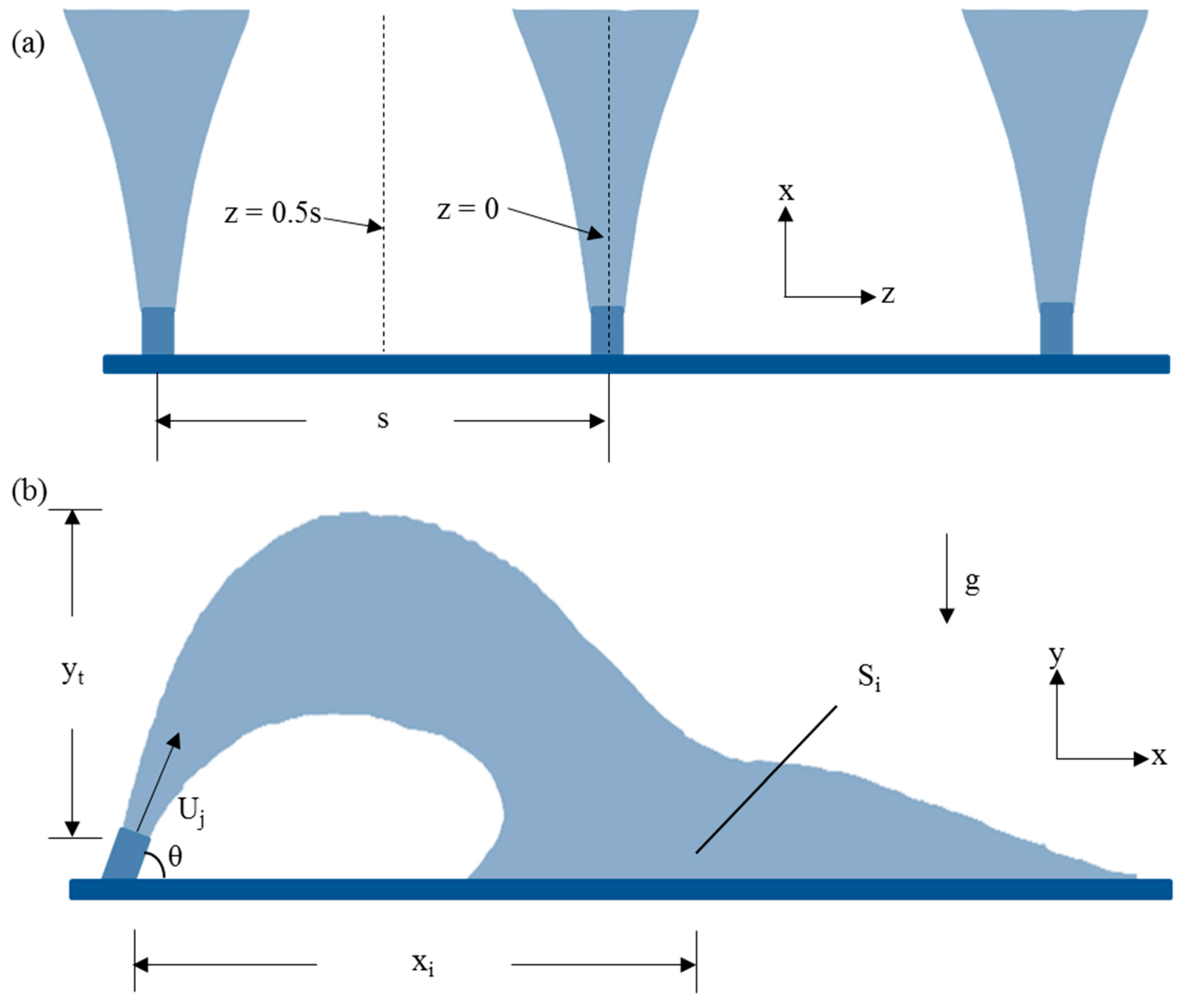
A schematic plot of multiple inclined dense jets is presented in Figure 1. The jets are ejected into the ambient water with an initial velocity of Uj from multiple ports with a spacing of s. The jets leave the nozzle at an angle of θ, reach the highest location, and fall back to the horizontal bed. The highest height is hereafter referred to as the terminal right height (yt), the length between the diffuser nozzle and the return point is referred to as the impact distance (xi), and the dilution at the return point is referred to as the impact dilution (Si).
The dilution characteristics of a single dense jet are primarily governed by the discharge volume flux Q, kinematic momentum flux M, and buoyancy flux B, which are defined as [2,3,4,31]
where d is the port diameter; Uj is the initial jet velocity; g’ is the reduced gravitational acceleration, which is equal to gravitational acceleration times initial density difference divided by the ambient water density. These variables can also be utilized to determine the jet’s Reynolds number, R = Ujd/ν, where ν is the kinematic viscosity.
Following a dimensional analysis, yt can be expressed as
where LM and LQ are two length scales, which can be expressed as
This is equivalent to
where F is the densimetric Froude number, defined as
Similarly, xi and Si can be expressed as
This study only investigates jets discharged at the angle of 60°, because this angle is widely recognized as the optimal angle [2,3], and thus the effects of the jet angle are not considered here. For multiple jets, the port spacing s should be considered. Therefore, yt, xi, and Si could be expressed as
2.2. Governing Equations
The present study assumes that the multiple fluids are incompressible and Newtonian. The viscosity and density of the fluids were assumed to be constant, and those of the mixed fluid depend on the fraction of the fluids. These assumptions were considered valid for the present cases. The three-dimensional Navier–Stokes equations for multiphase fluids can be written as [32,33]:
with:
where t is time, U is velocity, ρ is density, prgh is static pressure minus hydraulic pressure, h is height of fluid column, g is gravitational acceleration, α is volume fraction, μ is dynamic viscosity, μt is turbulent viscosity, and subscript i denotes either fluid 1 or 2. In the current model, Fluids 1 and 2 represent the jet and ambient water, respectively.
The volume fraction of a fluid is represented by the variable α, and the diffusion equation can be expressed as:
where Dab is the molecular diffusivity, νt is the turbulent eddy viscosity, and SC is the turbulent Schmidt number.
2.3. Turbulence Modeling
The present paper focuses on two turbulence models: the standard k-ε and RNG k-ε. The standard k-ε turbulence closure is given by:
with
where k is the turbulent kinetic energy, ε is the turbulent energy dissipation rate, G is the production of turbulence due to shear, σε, c1ε, c2ε, cμ are model constants equal to 1.3, 1.44, 1.92, and 0.09, respectively.
The RNG k-ε turbulence closure is similar to the standard closure, but an additional term is included in the ε-equation:
with
where σk, σε, c1ε, c2ε, cμ, η0, and β are model constants equal to 0.71942, 0.71942, 1.42, 1.68, 0.0845, and 0.012, respectively.
2.4. Model Setup
The governing equations were solved using the solver named “twoLiquidMixingFoam” in OpenFOAM, which is a transient solver for multiphase fluids. It has been proven to be accurate for predicting the mixing behaviors of wastewater jets [24,34], but has rarely been validated for multiple inclined dense jets. The temporal term was discretized using the Euler scheme. The gradient term and Laplacian terms were discretized using the Gauss linear scheme. The divergence terms were discretized using the Gauss linear, Gauss vanLeer, and Gauss upwind schemes. The linear method was used for interpolation schemes. An iterative solver for symmetric and asymmetric matrices, which uses a run-time selected smoother to converge the solution to the required tolerance, was used for the velocity field; to reduce the mesh dependency of the numbers of iterations, the Gauss Seidel technique was utilized, which is an improved version of the Jocobi method. Further information regarding these algorithms can be found in [3]. The tolerances for the fraction of fluids, pressure, and velocity fields were 1 × 10⁻⁹, 1 × 10⁻⁷, 1 × 10⁻⁷, respectively.
There are two sets of planes of symmetry in the present cases: One set goes through the centers of the jets, and the other goes through the midpoints between two adjacent jets. Therefore, in all simulations, the computational domains extended from z = 0 to z = s/2 in the z direction (Figure 1), and the symmetric boundary function available in OpenFOAM was assigned to the boundary patches corresponding to the planes of symmetry. A preliminary study showed that the results obtained by a model with four complete jets simulated were almost identical to the current one, but the computational costs were more than ten times higher. The “Reflect” function in ParaView was utilized to mirror the data across the planes of symmetry, and thus the final numerical datasets contained three complete jets. Preliminary tests found that the results in the area of interest were insensitive to the types of wall boundary conditions (slip or no-slip) for the bottom wall, so the slip boundary condition was used to speed up the simulations. The standard wall function “nutkWallFunction” in OpenFOAM was utilized for the wall boundaries. The velocity inlet boundary condition was assigned to the port surfaces. The top patch and the patch located farthest in the x direction from nozzle were set as “inlet-outlet”, which is a boundary type available in OpenFOAM that automatically assigns the zero-gradient open boundary condition to the boundary patch when there is no backward flow and assigns the fixed-value boundary condition when there is backward flow, and the fixed value was set to be zero.
A refined mesh with hexahedral cells was utilized to discretize the computational area. The cell sizes ranged from 0.001 m near the jet inlet to 0.005 m far from the inlet. The number of computational cells for the cases with port spacing of 0.114 m was 194,400, and that for the cases with port spacing of 0.057 m was 113,400. The mesh resolution was determined based on grid independence studies, following the procedures described by Yan and Mohammadian [27]. For example, the difference between the results obtained by the current mesh (with 194,400 cells) and a much coarser mesh (with 155,520 cells) was less than 3%, and thus the current mesh resolution was considered satisfactory. The grids were very similar to those described in previous studies [26,27], so they are not presented here for the sake of brevity. The default time step was set as 0.005 s, but the “adjustTimeStep” function in OpenFOAM was turned on, which can automatically adjust the time step during the simulation according to the maximum Courant number. To ensure a small time step, the maximum Courant number was set as 0.5. The results were insensitive to the default time step. The present solver is a transient instead of a steady-state solver, so the simulations terminated according to the user-defined end time instead of the convergence criteria. The simulated fields became almost stable at around 60 s; to be conservative, all the simulations were run up to 210 s, and the results at the last 90 s were averaged to get the averaged outputs. Each simulation was performed using 16 parallel computations. The parameters of the simulated cases are summarized in Table 1.
3. Results
3.1. General Observations
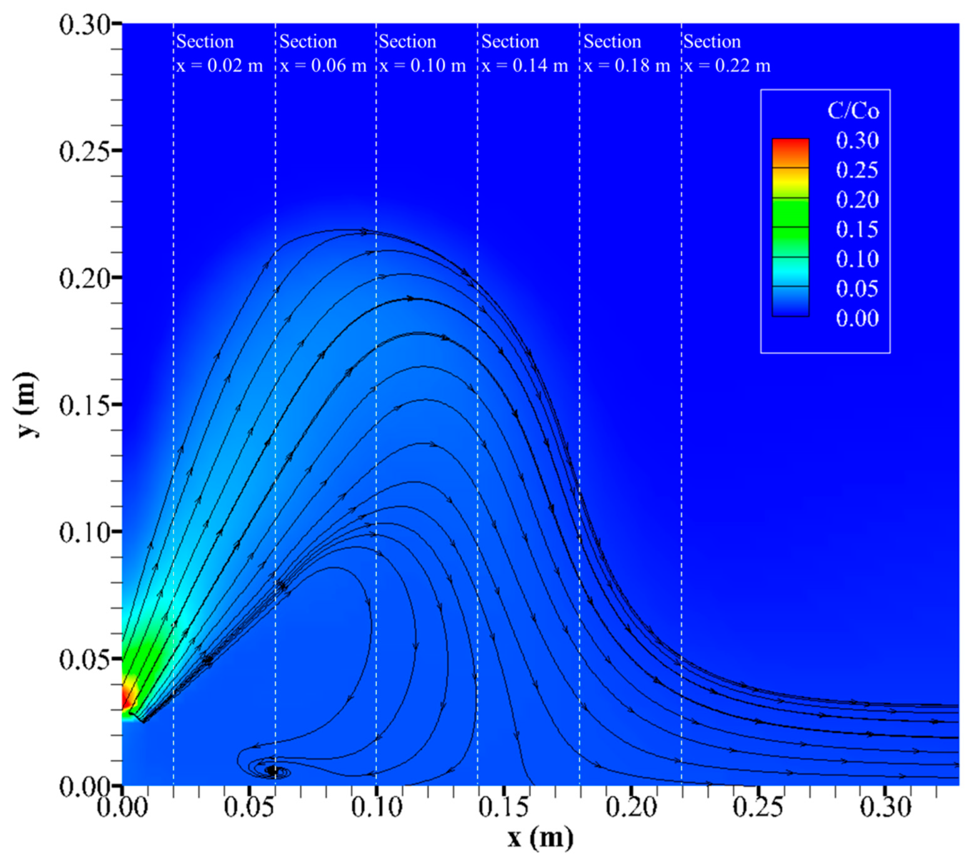
Figure 2 shows the normalized concentration field at the central plane for the case C1 (F = 62.9, and s/(d·F) = 0.94) obtained by the RNG k-ε model. In the figure, C denotes the concentration, and Co denotes the initial concentration of the jets. The flow streamlines were also plotted in the figure to better visualize the jet. As can be seen in Figure 2, the jets were ejected into the ambient water at an angle of 60°, and the ambient water was entrained into the jets because of the shear stress. The jets were continuously diluted along their trajectories because of the jet spread and water entrainment. At the early stage when the jets were rising, the vertical component of the jet velocities decreased, because the jets were denser than the receiving water, and the jets transferred their momentum to the ambient flow. After the jets reached the terminal rise height, the vertical component of the jet velocities became negative, and thus the jets started falling back towards the bed. The horizontal component of the jet velocities continuously decreased because of the shear stress between the jets and the ambient water. Therefore, the jets roughly moved along a parabolic curve. After the jets reached the bed, they moved as bottom density currents. The overall pattern of flow and mixing processes of multiple inclined dense jets at the central plane in the streamwise and vertical directions was similar to those of single jets, and was qualitatively in accordance with the general observations from the experiments reported by Abessi and Roberts [2].
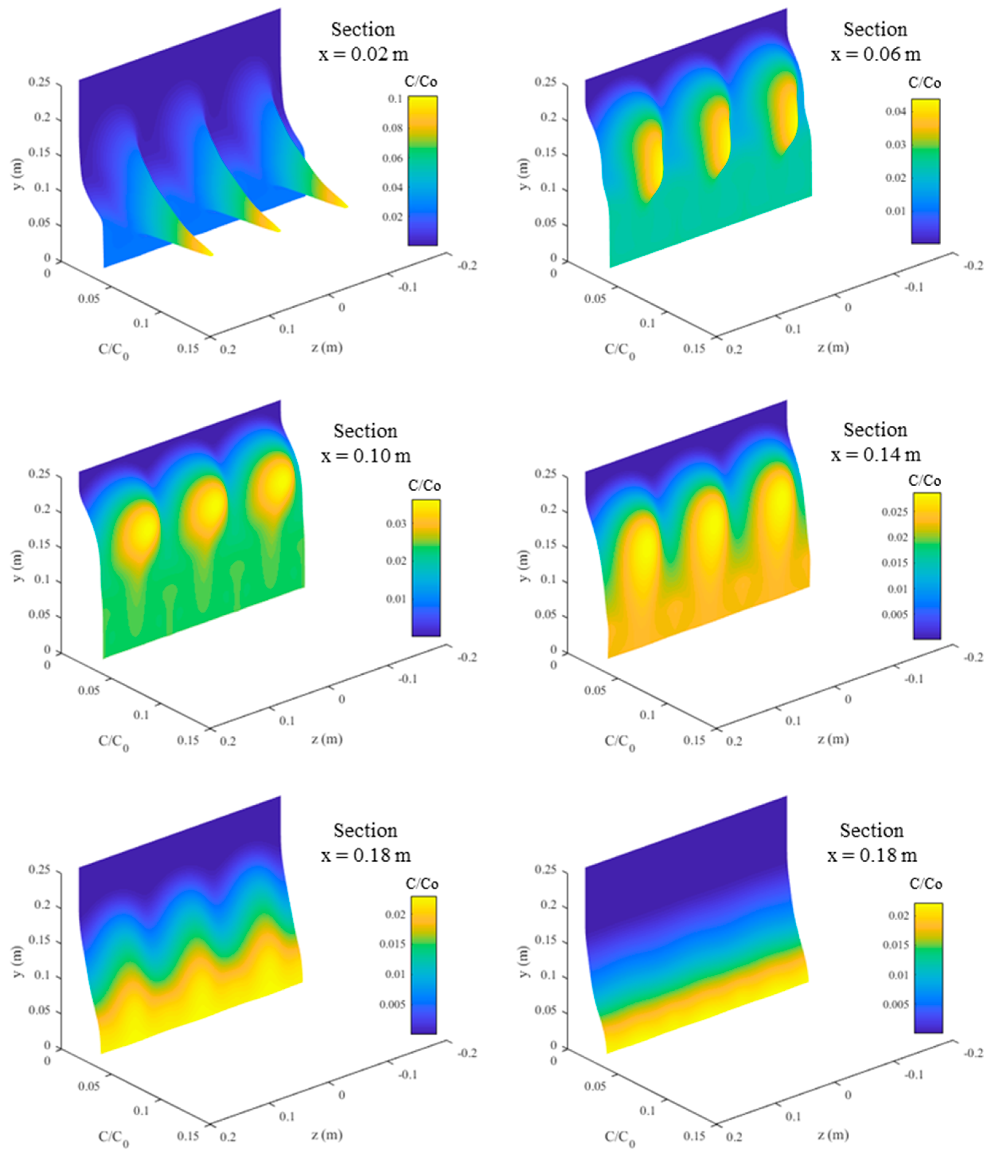
Figure 3 presents the concentration fields at various sample downstream locations for the case C1 (F = 62.9, and s/(d·F) = 0.94) obtained by the RNG k-ε model. The streamwise locations of these sections have been shown in Figure 2. As can be seen in the figure, at the cross sections close to the nozzles (such as x = 0.02 m), the jets behaved like individual single jets, and the concentration values suddenly dropped from the jet centerlines to the ambient locations. The jets were continuously diluted by the ambient water, and thus the centerline concentrations gradually decreased as the jets moved further. The jets also spread in the lateral direction, and thus the jets gradually interacted with each other. At moderate downstream locations (such as x = 0.10 m), the jets were still identifiable, but they were obviously interacting with each other, and the differences in concentration between the peaks and ambient locations became less significant. At farther cross sections (such as x = 0.22 m), the jets were completely mixed in the lateral direction and the individual jets were not identifiable, acting like a slot jet. These general observations from the numerical simulations were in accordance with the experimental observations [2], demonstrating that the numerical model can capture the overall flow and mixing properties of multiple inclined dense jets very well.
In addition to the model accuracy, computational efficiency is also an important factor for evaluating a model’s performance. The averaged computational costs of the simulations with the standard and RNG k-ε models were 36.57 and 36.68 hours, so the RNG k-ε model did not significantly increase the computational costs for the present cases. Therefore, the computational efficiency of the two models for the present cases can be regarded to be very close, and is thus not considered in subsequent sections.
3.2. Terminal Rise Height
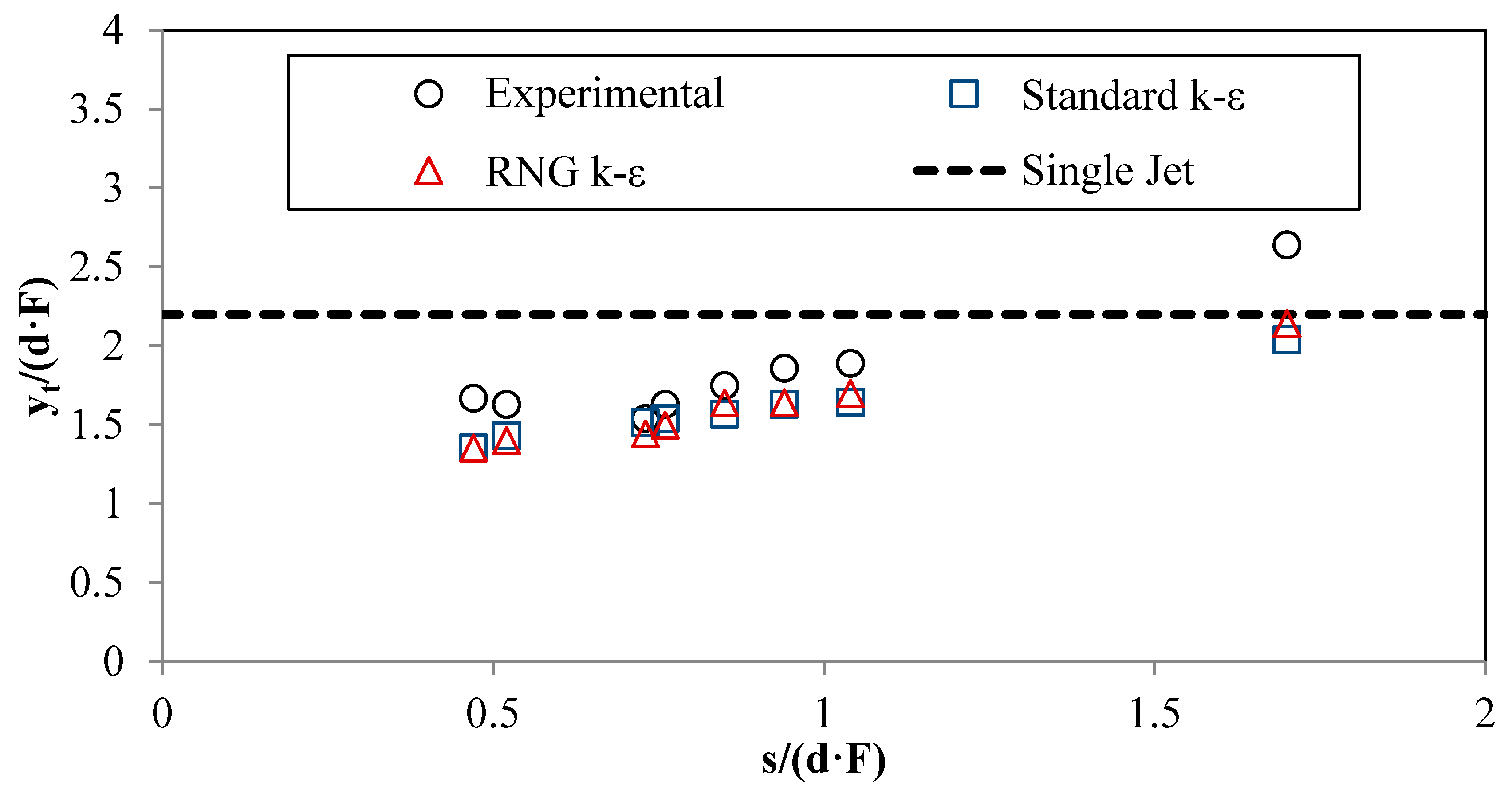
Figure 4 compares the results of yt/(d·F) for the eight cases considered in this paper obtained from the experiments and numerical simulations. In the figure, the results of yt/(d·F) are plotted against the values of s/(d·F) for the convenience of showing the effects of the port spacing. The results for single discharges calculated from the empirical equations proposed by Roberts et al. [35] were also plotted in the same figure. As can be seen, the values of yt/(d·F) generally increased with increasing values of s/(d·F), which is in agreement with the experimental observations for multiple inclined dense jets discharged from moderately spaced ports [2]. The phenomenon that the values of yt/(d·F) increased with increasing values of s/(d·F) can be explained by the Coanda effect; namely, the entrainment of ambient water into the jets is less restricted for the multiple jets with greater port spacing, and thus the dilution is higher, resulting in greater values of yt/(d·F).
The numerical models predicted the values of yt/(d·F) very well, except for case C5, in which the normalized port spacing is quite large. Theoretically, the mixing behaviors of multiple jets with infinitely large port spacing should be identical to those of single jets, and the values of yt/(d·F) generally increase with increasing port spacing, so the solutions of yt/(d·F) for single jets should be the largest possible values. The markers corresponding to the numerical results for case C5 were lower than the line for the empirical solutions for the single jet case, implying that the present numerical results are consistent with the experiments reported by Roberts et al. [35]. Overall, the markers corresponding to the RNG k-ε model are quite close to those corresponding to the experimental data, showing the good prediction ability of the RNG k-ε closure. The symbols for the standard k-ε model were roughly close to those for the RNG k-ε model, because most of the terms in the two closures were the same. However, the results obtained by the standard k-ε model departed farther from the data.
To quantitatively evaluate the two numerical closures, various fit measurements, including the mean bias error (MBE), mean absolute error (MAE), mean absolute percentage error (MAPE), root-mean-squared error (RMSE), normalized root-mean-squared error (NRMSE), and coefficient of determination (R2), were calculated (Table 2). It should be noted that the size of each data sample was relatively small, so the relative measure of fit, R2, may not be able to provide very meaningful conclusions. Both Figure 4 and Table 2 show that the RNG k-ε model predicted better results than the standard k-ε model. Based on the value of MAPE, the errors for the numerical results were well below 15%, so the model accuracy was acceptable for practical purposes.
3.3. Impact Distance
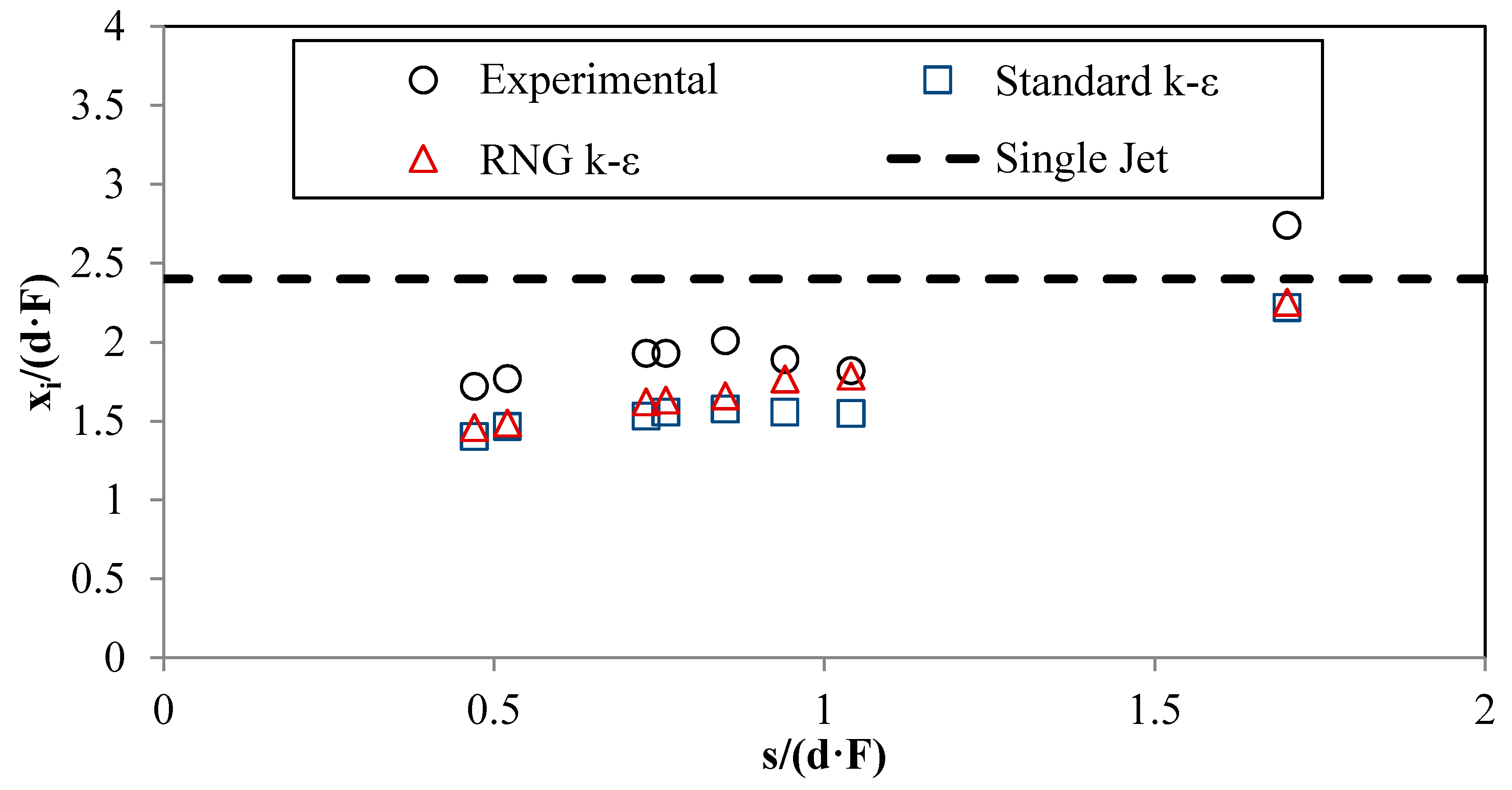
The results of xi(d·F) for the cases considered in this study obtained from the experiments and numerical simulations are shown in Figure 5, and the solutions for point discharges are also plotted in the same figure. As can be seen, the values of xi/(d·F) generally increased with increasing values of s/(d·F), which can also be explained by the Coanda effect mentioned earlier.
The numerical results of xi/(d·F) showed a good match with the experimental results [2]. Similar to the comparisons for yt/(d·F), the match for case C5 was relatively poor. However, the numerical results were smaller than the empirical solutions for the single jet, which were expected to be the upper limit of possible values, so the current numerical results were in accordance with those of Roberts et al. [35]. Generally, the results obtained by the RNG k-ε model were quite close to measurements, demonstrating the prediction capability of the RNG k-ε model for multiple inclined dense jets discharged from moderately spaced ports. The results obtained by the standard k-ε model were similar to those obtained by the RNG k-ε model, but showed larger differences from the experimental measurements. Table 3 lists the results for error analyses. Both Figure 5 and Table 3 show that the RNG k-ε model predicted better results than the standard k-ε model. According to the values of MAPE, the errors for the results obtained by the standard k-ε model exceeded 15%, whereas those by the RNG k-ε model were within 15%.
3.4. Impact Dilution
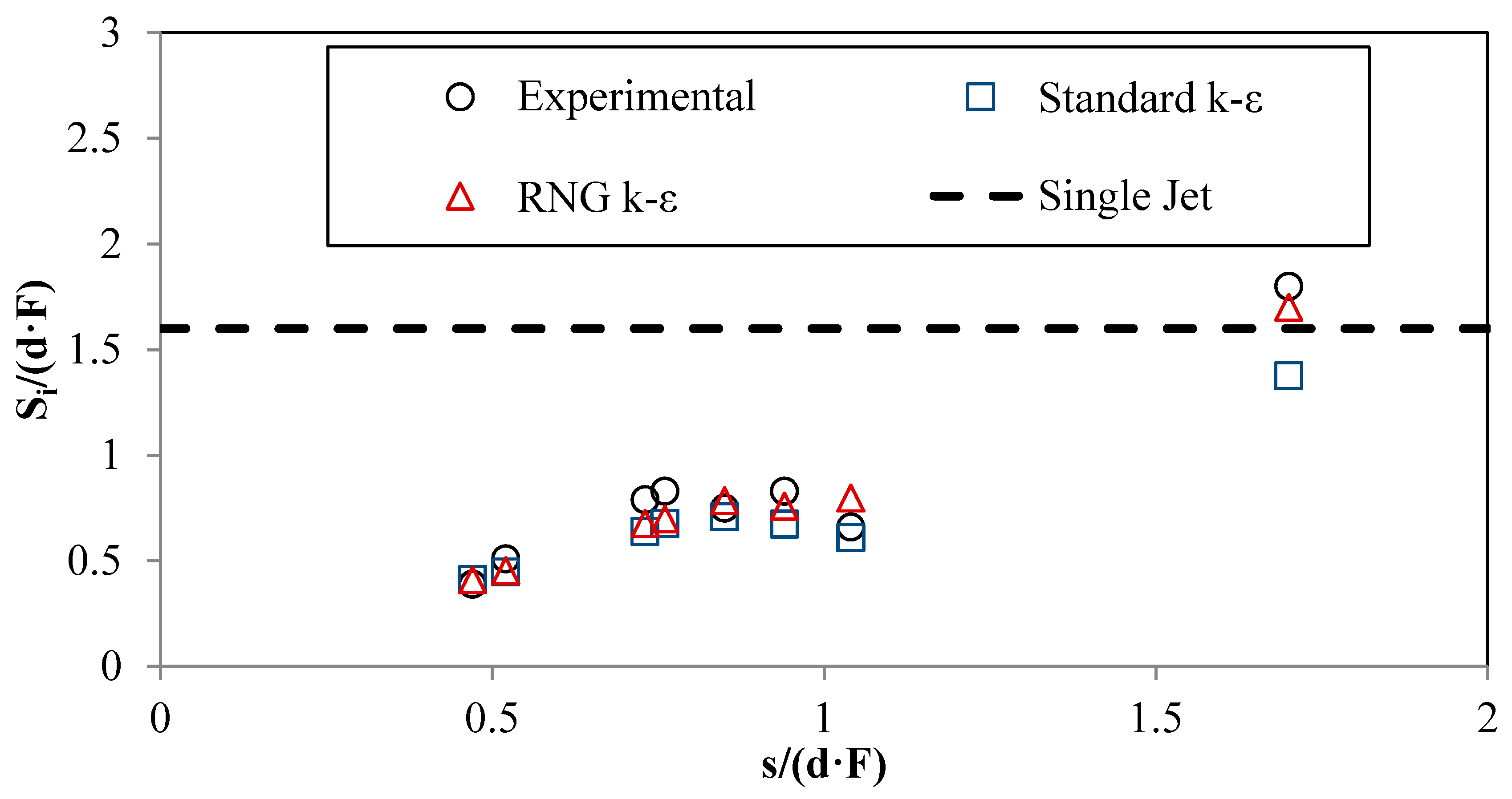
The results of Si/(d·F) obtained from the experiments and numerical simulations for the eight cases were plotted against the normalized port spacing in Figure 6. Similar to the geometrical features (yt and xi), the impact dilution also increased when the port spacing increased. The agreements between the experimental and numerical results were satisfactory, demonstrating that the numerical model can satisfactorily predict the impact dilution for multiple inclined dense jets. The various fit measures were calculated and summarized in Table 4. The plots shown in Figure 6 and error indices summarized in Table 4 show that the RNG k-ε model predicted better results than the standard k-ε model, and both models provided predictions with errors smaller than 15%.
4. Discussion
The main contribution of the present study is the validation of the three-dimensional numerical model, based on the Reynolds-averaged Navier–Stokes equations, in predicting the mixing features of inclined dense jets discharged from moderately spaced ports. As shown in the results section, both the standard and RNG k-ε models provided satisfactory results. Therefore, the models can be further utilized to carry out additional computations for both academic and practical purposes. To the authors’ knowledge, this is the first time that multiple inclined dense jets have been successfully modeled using a three-dimensional numerical model.
It is acknowledged that there are several other popular and advantageous approaches for studying the mixing properties of wastewater effluents, such as the jet integral [36], entrainment restriction, and superposition approaches [13]. Such methods are very beneficial, if applicable, because they are typically simpler and less time-consuming. However, these methods have not been proven to be effective for multiple inclined dense jets, partially because the mechanics of such jets are very complicated, and are thus difficult to be conceptualized by simplified approaches. Yan and Mohammadian [19,20] successfully predicted the mixing properties of multiple inclined dense jets utilizing the multi-gene genetic programming approach, but models based on artificial intelligence or regression-based approaches still require more experimental or physical-based numerical data for improvement or extension, otherwise their predictions for the cases with parameters out of the training range might be unreliable. Therefore, demonstrating the performance of a numerical model for multiple inclined dense jets, which is a major contribution of the present study, is quite meaningful.
The major disadvantage of a three-dimensional model compared with the other approaches is the high computational cost. However, the present study proved that this is not a concern for the cases considered here, because the computational time was just about 36.5 hours, which is acceptable for practical design of outfall systems or environmental impact assessments. The computational time of the simulations based on OpenFOAM is not a concern, because it can be dramatically reduced if needed. First, the simulations can be performed using parallel computations, and the computational costs can be further reduced with more computing resources. Second, despite the fact that the phenomenon and simulations are three-dimensional, appropriate simplifications can be utilized; for example, the present simulations only covered the region between two adjacent planes of symmetry rather than the whole domain, and so the computational domain became much smaller. Third, refined mesh can be utilized, with finer mesh being utilized for the area of interest, and coarser mesh for other areas.
The present study demonstrated that the RNG k-ε turbulence closure is generally more accurate than the standard one. Both the standard and RNG k-ε models are two-transport-equation models. One transport equation was the k equation, and the other is the ε equation. These two equations both relate the Reynolds stresses to the mean velocity gradients and νt using the gradient diffusion hypothesis. The RNG k-ε turbulence closure outperformed the standard one in modeling multiple inclined dense jets, probably due to three reasons: 1) the RNG k-ε turbulence closure calculates νt using the scale elimination procedure, which takes into account the modification of effective turbulent transport due to the Reynolds number; 2) the RNG k-ε turbulence closure calculates the inverse effective Prandtl numbers using a RNG-based formula, which is of a lower level of simplification; and 3) the RNG k-ε turbulence closure improved the ε equation by adding an additional term, which can more accurately calculate νt.
It is acknowledged that there are a large number of different turbulence closures, and some closures may perform even better, such as DNS and LES. However, the most suitable model should be determined by considering accuracy and efficiency simultaneously, which are normally conflicting. The standard k-ε turbulence model has been widely accepted to have a good balance between accuracy and efficiency, and is therefore very popular. A more accurate model is typically more complicated, whereas a simpler model is typically less accurate than the standard k-ε turbulence model. The present study found that the RNG k-ε turbulence model can outperform the standard model in performance without sacrificing the efficiency, as it does not obviously increase the computational costs, and is thus a better option.
5. Conclusions
Numerical simulations for multiple inclined dense jets discharged from moderately spaced ports were performed, and the numerical results provided by the standard and RNG k-ε models were compared to experimental data. The results showed that the three-dimensional numerical model can reproduce satisfactory results for multiple inclined dense jets. Both the standard and RNG k-ε models can provide results of terminal rise height and impact dilution with errors smaller than 15%. The modeled results of the impact distance from the standard k-ε model departed more than 18% from the measurements, but those from the RNG k-ε model were within the 15% range. The averaged computational costs of the simulations with the standard and RNG k-ε models were 36.57 and 36.68 hours, so the RNG k-ε model did not significantly increase the computational costs for the present cases. Therefore, and RNG k-ε model is more accurate than the standard model without sacrificing the efficiency, and is thus recommended as a better option for modeling multiple inclined dense jets. The present study aims to validate the performance of the numerical model in simulating multiple inclined dense jets. In subsequent studies, the validated model will be utilized to carry out additional computations to investigate the effects of the jet inclination, flowing currents, and stratification on the mixing behaviors.
Author Contributions
Conceptualization and analysis, X.Y. and A.M.; writing—original draft preparation, X.Y.; writing—review and editing, A.M.; supervision and project administration, A.M.
Funding
This work was funded by the Natural Sciences and Engineering Research Council of Canada (NSERC Discovery Grants). The first author received a scholarship from the China Scholarship Council (CSC).
Conflicts of Interest
The authors declare no conflict of interest.
References
- Shao, D.; Law, A.W.K. Boundary impingement and attachment of horizontal offset dense jets. J. Hydro-Environ. Res. 2011, 5, 15–24. [Google Scholar] [CrossRef]
- Abessi, O.; Roberts, P.J. Multiport diffusers for dense discharges. J. Hydraul. Eng. 2014, 140, 04014032. [Google Scholar] [CrossRef]
- Abessi, O.; Roberts, P.J. Multiport diffusers for dense discharge in flowing ambient water. J. Hydraul. Eng. 2017, 143, 04017003. [Google Scholar] [CrossRef]
- Abessi, O.; Roberts, P.J. Rosette Diffusers for Dense Effluents in Flowing Currents. J. Hydraul. Eng. 2017, 144, 06017024. [Google Scholar] [CrossRef]
- Shrivastava, I.; Adams, E.E. Pre-dilution of desalination reject brine: Impact on outfall dilution in different water depths. J. Hydro-environ. Res. 2019, 24, 28–35. [Google Scholar] [CrossRef]
- Jiang, M.; Law, A.W.K.; Zhang, S. Mixing behavior of 45 inclined dense jets in currents. J. Hydro-Environ. Res. 2018, 18, 37–48. [Google Scholar] [CrossRef]
- Oliver, C.J.; Davidson, M.J.; Nokes, R.I. Removing the boundary influence on negatively buoyant jets. Environ. Fluid Mech. 2013, 13, 625–648. [Google Scholar] [CrossRef]
- Lyu, S.; Seo, I.W.; Do Kim, Y. Experimental investigation on behavior of multiple vertical buoyant jets discharged into a stagnant ambient. KSCE J. Civil Eng. 2013, 17, 1820–1829. [Google Scholar] [CrossRef]
- Wang, H.J.; Davidson, M.J. Jet interaction in a still ambient fluid. J. Hydraul. Eng. 2003, 129, 349–357. [Google Scholar] [CrossRef]
- Knystautas, R. The turbulent jet from a series of holes in line. Aeronaut. Q. 1964, 15, 1–28. [Google Scholar] [CrossRef]
- Liseth, P. Mixing of merging buoyant jets from a manifold in stagnant receiving water of uniform density. In Advances in water pollution research. In Advances in Water Pollution Research Proceedings of the 6th International Conference, Jerusalem, Israel, 18–23 June 1972; Pergamon Press: Oxford, UK, 1973; pp. 921–936. [Google Scholar]
- Shinneeb, A.M.; Balachandar, R.; Bugg, J.D. Confinement effects in shallow-water jets. J. Hydraul. Eng. 2010, 137, 300–314. [Google Scholar] [CrossRef]
- Yannopoulos, P.C.; Noutsopoulos, G.C. Interaction of vertical round turbulent buoyant jets—Part I: Entrainment restriction approach. J. Hydraul. Res. 2006, 44, 218–232. [Google Scholar] [CrossRef]
- Adams, E.E. Submerged Multiport Diffusers in Shallow Water with Current. Master’s Thesis, Massachusetts Institute of Technology, Cambridge, MA, USA, 1972. [Google Scholar]
- Shrivastava, I.; Adams, E.E. Mixing of Tee Diffusers in Shallow Water with Crossflow: A New Look. J. Hydraul. Eng. 2019, 145, 04019006. [Google Scholar] [CrossRef]
- Xu, Z.; Otoo, E.; Chen, Y.; Ding, H. 2D PIV Measurement of Twin Buoyant Jets in Wavy Cross-Flow Environment. Water 2019, 11, 399. [Google Scholar] [CrossRef]
- Hodgson, J.E.; Moawad, A.K.; Rajaratnam, N. Concentration field of multiple circular turbulent jets. J. Hydraul. Res. 1999, 37, 249–256. [Google Scholar] [CrossRef]
- Lai, A.C.; Lee, J.H. Dynamic interaction of multiple buoyant jets. J. Fluid Mech. 2012, 708, 539–575. [Google Scholar] [CrossRef]
- Yan, X.; Mohammadian, A. Multigene Genetic-Programming-Based Models for Initial Dilution of Laterally Confined Vertical Buoyant Jets. J. Mar. Sci. Eng. 2019, 7, 246. [Google Scholar] [CrossRef]
- Yan, X.; Mohammadian, A. Evolutionary modeling of inclined dense jets discharged from multiport diffusers. J. Coast. Res. 2019, in press. [Google Scholar] [CrossRef]
- Wang, R.Q.; Law, A.W.K.; Adams, E.E.; Fringer, O.B. Large-eddy simulation of starting buoyant jets. Environ. Fluid Mech. 2011, 11, 591–609. [Google Scholar] [CrossRef]
- Kheirkhah Gildeh, H.; Mohammadian, A.; Nistor, I.; Qiblawey, H.; Yan, X. CFD modeling and analysis of the behavior of 30° and 45° inclined dense jets—New numerical insights. J. Appl. Water Eng. Res. 2016, 4, 112–127. [Google Scholar] [CrossRef]
- Kheirkhah Gildeh, H.; Mohammadian, A.; Nistor, I.; Qiblawey, H. Numerical modeling of 30° and 45° inclined dense turbulent jets in stationary ambient. Environ. Fluid Mech. 2015, 15, 537–562. [Google Scholar] [CrossRef]
- Zhang, S.; Jiang, B.; Law, A.W.K.; Zhao, B. Large eddy simulations of 45 inclined dense jets. Environ. Fluid Mech. 2016, 16, 101–121. [Google Scholar] [CrossRef]
- Alfaifi, H.; Mohammadian, A.; Gildeh, H.K.; Gharavi, A. Experimental and numerical study of the characteristics of thermal and nonthermal offset buoyant jets discharged into stagnant water. Desalin. Water Treat. 2019, 141, 171–186. [Google Scholar] [CrossRef]
- Kheirkhah Gildeh, H.; Mohammadian, A.; Nistor, I.; Qiblawey, H. Numerical modeling of turbulent buoyant wall jets in stationary ambient water. J. Hydraul. Eng. 2014, 140, 04014012. [Google Scholar] [CrossRef]
- Zhang, S.; Law, A.W.K.; Zhao, B. Large eddy simulations of turbulent circular wall jets. Int. J. Heat Mass Transf. 2014, 80, 72–84. [Google Scholar] [CrossRef]
- Zhang, S.; Law, A.W.K.; Jiang, M. Large eddy simulations of 45° and 60° inclined dense jets with bottom impact. J. Hydro-environ. Res. 2017, 15, 54–66. [Google Scholar] [CrossRef]
- Yan, X.; Mohammadian, A. Numerical Modeling of Vertical Buoyant Jets Subjected to Lateral Confinement. J. Hydraul. Eng. 2017, 143, 04017016. [Google Scholar] [CrossRef] [Green Version]
- Lou, Y.; He, Z.; Jiang, H.; Han, X. Numerical simulation of two coalescing turbulent forced plumes in linearly stratified fluids. Phys. Fluids 2019, 31, 037111. [Google Scholar]
- Fischer, H.B.; List, E.J.; Koh, R.C.H.; Imberger, J.; Brooks, N.H. Mixing in Inland and Coastal Waters; Academic Press: New York, NY, USA, 1979. [Google Scholar]
- Holzmann, T. Mathematics, Numerics, Derivations and OpenFOAM®; Holzmann CFD: Loeben, Germany, 2016. [Google Scholar]
- OpenFOAM User Guide; Version 4.0; The OpenCFD Foundation: London, UK, 2016.
- Lai, A.C.; Zhao, B.; Law, A.W.K.; Adams, E.E. A numerical and analytical study of the effect of aspect ratio on the behavior of a round thermal. Environ. Fluid Mech. 2015, 15, 85–108. [Google Scholar] [CrossRef]
- Roberts, P.J.; Ferrier, A.; Daviero, G. Mixing in inclined dense jets. J. Hydraul. Eng. 1997, 123, 693–699. [Google Scholar] [CrossRef]
- Fang, S.; Chen, Y.; Xu, Z.; Otoo, E.; Lu, S. An Improved Integral Model for a Non-Buoyant Turbulent Jet in Wave Environment. Water 2019, 11, 765. [Google Scholar] [CrossRef]
Figure 1.
Schematic of multiple inclined dense jets: (a) plan view; (b) elevation view.

Figure 2.
Concentration fields at the central plane; Case C1, F = 62.9, and s/(d·F) = 0.94.

Figure 3.
Concentration fields at various downstream locations; Case C1, F = 62.9, and s/(d·F) = 0.94.
Figure 3.
Concentration fields at various downstream locations; Case C1, F = 62.9, and s/(d·F) = 0.94.

Figure 4.
Experimental and numerical results of yt/(d·F).

Figure 5.
Experimental and numerical results of xi/(d·F).

Figure 6.
Experimental and numerical results of Si/(d·F).


Table 1.
Parameters of the simulated cases.
| Cases | d (mm) | s (mm) | F (—) | s/(d·F) (—) |
|---|---|---|---|---|
| C1 | 1.93 | 114 | 62.9 | 0.94 |
| C2 | 1.93 | 114 | 56.8 | 1.04 |
| C3 | 1.93 | 114 | 77.3 | 0.76 |
| C4 | 1.93 | 114 | 81.1 | 0.73 |
| C5 | 1.93 | 57 | 17.3 | 1.71 |
| C6 | 1.93 | 57 | 34.7 | 0.85 |
| C7 | 1.93 | 57 | 63.1 | 0.47 |
| C8 | 1.93 | 57 | 56.8 | 0.52 |
Note: d = port dimeter; s = port spacing; F = densimetric Froude number.
Table 2.
Error indices of the numerical models for yt/(d·F).
| Model | MBE | MAE | MAPE (%) | RMSE | NRMSE (%) | R2 |
|---|---|---|---|---|---|---|
| Standard k-ε | −0.24 | 0.24 | 12.10 | 0.29 | 0.16 | 0.88 |
| RNG k-ε | −0.22 | 0.22 | 11.81 | 0.26 | 0.14 | 0.91 |
Table 3.
Error indices of the numerical models for xi/(d·F).
| Model | MBE | MAE | MAPE (%) | RMSE | NRMSE (%) | R2 |
|---|---|---|---|---|---|---|
| Standard k-ε | −0.37 | 0.37 | 18.56 | 0.38 | 0.19 | 0.98 |
| RNG k-ε | −0.27 | 0.27 | 13.26 | 0.30 | 0.15 | 0.84 |
Table 4.
Error indices of the numerical models for Si/(d·F).
| Model | MBE | MAE | MAPE (%) | RMSE | NRMSE (%) | R2 |
|---|---|---|---|---|---|---|
| Standard k-ε | −0.13 | 0.13 | 13.82 | 0.18 | 0.22 | 0.99 |
| RNG k-ε | −0.04 | 0.08 | 10.76 | 0.09 | 0.11 | 0.96 |
© 2019 by the authors. Licensee MDPI, Basel, Switzerland. This article is an open access article distributed under the terms and conditions of the Creative Commons Attribution (CC BY) license (http://creativecommons.org/licenses/by/4.0/).
Share and Cite
MDPI and ACS Style
Yan, X.; Mohammadian, A. Numerical Modeling of Multiple Inclined Dense Jets Discharged from Moderately Spaced Ports. Water 2019, 11, 2077. https://doi.org/10.3390/w11102077
AMA Style
Yan X, Mohammadian A. Numerical Modeling of Multiple Inclined Dense Jets Discharged from Moderately Spaced Ports. Water. 2019; 11(10):2077. https://doi.org/10.3390/w11102077
Chicago/Turabian StyleYan, Xiaohui, and Abdolmajid Mohammadian. 2019. "Numerical Modeling of Multiple Inclined Dense Jets Discharged from Moderately Spaced Ports" Water 11, no. 10: 2077. https://doi.org/10.3390/w11102077
Note that from the first issue of 2016, this journal uses article numbers instead of page numbers. See further details here.