Using Soil Moisture Sensors for Automated Irrigation Scheduling in a Plum Crop
by
 , ,
, ,
Sandra Millán
1,* ,
,
Jaume Casadesús
2,
Carlos Campillo
1,
María José Moñino
1 and
Maria Henar Prieto
1 1
Centro de Investigaciones Científicas y Tecnológicas de Extremadura (CICYTEX), Finca La Orden, Junta de Extremadura, Autovía A-V, Km 372, 06187 Guadajira (Badajoz), Spain
2
Institut de Recerca i TecnologiaAgroalimentàries (IRTA), Fruitcentre, Parc de Gardeny, 25003 Lleida, Spain
*
Author to whom correspondence should be addressed.
Water 2019, 11(10), 2061; https://doi.org/10.3390/w11102061
Submission received: 5 September 2019
/
Revised: 26 September 2019
/
Accepted: 30 September 2019
/
Published: 2 October 2019
(This article belongs to the Special Issue Optimization of Irrigation Scheduling: Challenges and Perspectives)
Abstract
:The growing scarcity and competition for water resources requires the urgent implementation of measures to ensure their rational use. Farmers need affordable irrigation tools that allow them to take advantage of scientific know-how to improve water use efficiency in their common irrigation practices. The aim of this study is to test under field conditions, and adjust where required, an automated irrigation system that allows the establishment of regulated deficit irrigation (RDI) strategies in a stone fruit orchard. For this, an automated device with an algorithm which combines water-balance-based irrigation scheduling with a feedback adjustment mechanism using 15 capacitive sensors for continuous soil moisture measurement was used. The tests were carried out in 2016 and 2017 in Vegas Bajas del Guadiana (Extremadura, Spain) on an experimental plot of ‘Red Beaut’, an early-maturing Japanese plum cultivar. Three irrigation treatments were established: control, RDI and automatic. The control treatment was scheduled to cover crop water needs, a postharvest deficit irrigation (40% crop evapotranspiration (ETc)) strategy was applied in the RDI treatment, while the Automatic treatment simulated the RDI but without human intervention. After two years of testing, the automated system was able to “simulate” the irrigation scheduling programmed by a human expert without the need for human intervention.
1. Introduction
The demand for irrigation water in agricultural systems is an important area of concern, especially given the growing scarcity of available water resources and the need to compete with other consumer sectors [1]. Appropriate and efficient irrigation water management and use practices are urgently required and should be aimed at ensuring both economic and environmental benefits [2]. Crop water needs vary spatially and temporally depending on meteorological conditions, crop type and crop growth stage [3]. Spatial variability may be associated to soil texture changes, topographic features, soil compaction, fertility differences, local pest distribution, and the characteristics of the irrigation system employed [4,5,6,7,8]. Consequently, irrigation management efficiency depends to a large extent on the ability to adapt water inputs to the variable needs of the plants. A wide range of sensors are available on the market today which are able to provide real time information about the plant and its surroundings. However, the correct use of such information for decision-making purposes can be highly complex because of the need for specialist know-how and a considerable dedication of time and effort. Information and communication technologies (ICTs) can contribute to resolving this problem by facilitating the capture, storage, processing, and dissemination of significant amounts of information [9]. Integrating such technologies with what is known about plant response to water inputs at the different growth stages of a crop is a major challenge which, if overcome, could lead to the development of intelligent systems able to emulate the expert decision-making process.
Irrigation scheduling methods are classified in three major groups: water-balance-based methods, methods which focus on monitoring soil water content or potential, and methods which use measurement of the plant water status as reference [10,11]. Although the latter option may be the most attractive “a priori”, as it the plant itself which is giving information about its water needs, its practical application for irrigation management is still in a developmental stage [12].
The water balance method is the most commonly used strategy worldwide for irrigation scheduling. In this method, the soil-plant system water inputs must balance the expected outputs. The main water output, without considering the characteristics of the irrigation system, is through crop evapotranspiration (ETc) which, following the method proposed by the Food and Agriculture Organization of the United Nations (FAO), is calculated as the product of the evapotranspiration of the reference crop (ETo) and the crop coefficient (Kc) [13]. This method has the advantage of establishing a direct correlation between crop water needs and climate conditions [3]. However, it has the drawback of not considering any possible deviations between estimated and actual consumption values caused by the particular conditions of the plot, interannual variations in crop growth patterns [14], the plant material, or the crop practices undertaken [3]. Such mismatching can result in a systematic error that could accumulate over the crop cycle.
Interest in irrigation scheduling based on information provided by soil moisture sensors has been boosted by technological advances in sensorization and communications. These technological advances have led to commercial developments which are able to provide processed information with recommendations for the resetting of irrigation volumes. There are even more advanced options which offer full and complete system automation. However, the weaknesses of a control system based solely on sensors include the risk of sensor breakdown, measurement variability [15], and the difficulty of interpreting the sensor data, especially in the case of drip irrigation where soil water distribution is heterogenous [16].
There are a number of complementary benefits and drawbacks to scheduling irrigation on the basis of the water balance and the use of sensors. However, the automated combination of the two systems is a potential way of eliminating the drawbacks and enjoying the benefits of each. An optimized system could integrate the water balance calculations with meteorological data, together with a correction of the Kc value according to actual water consumption continuously assessed with soil sensors. This type of infrastructure would, in principle, be aimed at agricultural systems of high added value which require highly specialized management. This could be the case in the employment of regulated deficit irrigation (RDI) strategies in woody crops. An RDI strategy involves supplying an irrigation volume below the crop’s theoretical water requirements during specific periods of the crop cycle in phenological stages which are less sensitive to a water deficit [17]. The RDI strategies are based on the different seasonal or phenological sensitivity of some crops to water stress. They are used to save water resources and obtain agronomic benefits related to the control of plant vigor [18] and enhanced yield quality [19]. For Japanese plum, various RDI strategies have been proposed depending on the crop cycle [20,21].
The simplest systems which have been used in automated irrigation with soil moisture sensors or tensiometers are centered on initiating/terminating the irrigation when the measurements provided by the sensors rise above or fall below preestablished thresholds [22,23,24,25,26]. Cárdenas et al. [27] developed a system using soil moisture sensors which allowed the operator to choose a threshold above which the scheduled irrigation events were not permitted. An interesting approach for the development of automated systems is to combine ETc estimation with feedback of the information provided by the soil sensors, as in the case of direct measurement of plant consumption. Some authors have carried out such an integration using software tools and web applications [3,11,28,29]. The use of feedback is fundamental for the establishment of an automated control system [10]. There are two types of control systems: (1) open loop systems, in which the output is generated depending on the input or, in other words, no information or feedback is received about the state of the variable. The main drawback of an open loop system is that it cannot react to changes that occur in the system. (2) Closed loop systems, in which the output depends on considerations and corrections made by the feedback system or, in other words, the system controllers receive information about the state of the variable and calculate what future actions need to be taken [10]. With the second option, the sensors play an essential role in closing the cycle, as they obtain real time information about the plot.
The primary aim of this study is the adjustment and evaluation in field conditions of a fully automated irrigation system which integrates the water balance method with continuous soil moisture measurements and expert know-how of crop response to water deficit in ‘Red Beaut’, an early-maturing Japanese plum cultivar. A novel aspect of this work is the fact that the irrigation scheduling considers, among other things, the application of an RDI strategy specifically adapted to this crop and cultivar. The secondary objectives of this study include (i) securing adequate information for a better system adjustment, and (ii) checking the yield response of the trees against the RDI strategy creating an automated system
2. Materials and Methods
2.1. Study Area and Irrigation System
The study was carried out over the course of two crop seasons (2016–2017) in an early-maturing Japanese plum orchard of 1 ha (Prunus salicina Lindl. ‘Red Beaut’), located in “Finca La Orden”, an experimental farm in Badajoz, Spain (latitude 38°51′19.06″ N, longitude 6°40′18.90″ W, datum WGS84), run by the Scientific and Technological Research Centre of Extremadura (Regional Government of Extremadura). The trees were planted in the spring of 2005 with a 6 × 4 m spacing and in an east–west orientation.
A Mediterranean climate prevails in this area, with a dry season from June to September (summer) and a wet season from October to May (winter) with 80% of total precipitation. Mean annual precipitation is 500 mm and mean annual temperature is 16.5 °C (1992–2017).
Soil texture is loam, with an average 19.4% clay content, 40.2% lime content, and 40.4% sand content. The soil has a slightly acidic pH value, low organic material content and high apparent density, moderate to weak structure with normal P₂O₅ content (values above 40 ppm between soil depths of 0.4 and 0.6 m), low Na+ and K+ content, and low cation exchange capacity.
A drip-irrigation system was used, with one irrigation tape per row of trees located close to the base of the tree, with 4 × 4 l/h self-compensating emitters spaced at 1 m intervals.
2.2. Automatic Irrigation System
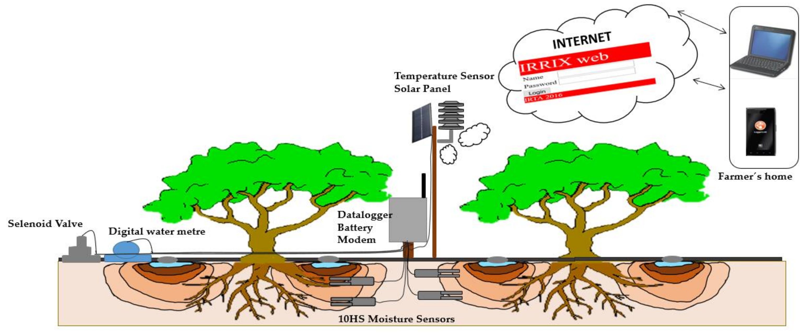
The automated irrigation system (Figure 1) was comprised of two fundamental components: (a) field equipment; and (b) the IRRIX software.
(a) Installation in the field of the following elements of the automated irrigation system:
- To monitor the soil moisture content in the experiment, fifteen 10HS capacitance probes (Decagon Devices Inc., Pullman, WA, USA) were installed in three representative trees. Five probes were installed in each tree: two probes under the emitter at 0.3 m depth, two probes under the emitter at 0.6 m depth and one probe situated between emitters, approximately at a distance of 0.15 m horizontally under the dripper line. The IRRIX software evaluated every probe and established the reference levels.
- An air temperature sensor (CS2015, Campbell Scientific Inc., Logan, UT, USA) at a height of 3 m (in line with a tree row).
- Energy source: next to the temperature probe, a solar panel was installed with a 12V-7Ah lead battery and voltage regulator (BlueSolar PWM-Pro, Victron Energy Blue Power, De Paal, The Netherlands).
- Sensors for irrigation water application control: a 24V-50Hz solenoid valve (Rain Bird Europe SCN, Aix-en-Provence, France), a digital water meter (MTK, Zenner, Madrid, Spain) and a relay controller (SMD-CD16AC, Campbell Scientific Inc., Logan, UT, USA).
- Logger: all the above components were connected to a datalogger (CR1000, Campbell Scientific Inc., Logan, UT, USA) which stored the data once every 5 min.
(b) IRRIX software.
IRRIX is a cloud-hosted web platform which, without the need for human intervention, carries out the following tasks:
- Captures data from the sensors installed in the field. The data were uploaded 4 times a day via IPv4/IPv6 to the IRRIX server.
- Data processing and interpretation: IRRIX analyzes all the input data to detect anomalies or important events in the system (irrigation, rain). As an indicator of the evolution of the soil’s water status, IRRIX is set for each sensor at the driest value recorded every day, soil water content (SWC), daily driest SWC (SWCd). Then, to reduce the variability between sensors, IRRIX normalizes these values specifically for each sensor, such as:where soil water content wilting point (SWCWP) and soil water content field capacity (SWCFC) correspond to the values that this sensor would take under conditions of wilting point and field capacity, respectively. In practice, SWCFC was taken at the beginning of the campaign from actual measurements of the system in field conditions, while SWCWP was assigned to the supposed value of SWC in wilting point for this type of soil.NSWCd = (SWCd − SWCWP)/(SWCFC − SWCWP)
To add the different sensors installed in the same irrigation sector, the system performs a weighted average where the weight of each sensor is the product of its reliability and representativeness. The reliability of a sensor is related to the quality of the data that a sensor is recording, in other words, whether the sensor is operating correctly or not due to some unexpected anomaly. IRRIX automatically estimates sensor reliability on a daily basis with a scale of values ranging from 0 to 1. All sensors have an initial value of 1, and each time an anomaly is detected the reliability value is decreased (multiplied by a value ranging between 0 and 0.5) depending on the seriousness of the anomaly. If the sensor stops working, IRRIX automatically removes it from the system (value of 0) and does not take the data from the sensor into account in its estimations. The representativeness of each sensor refers to whether the information provided by the sensor is relevant or not for the decision-making process in the irrigation control system. The representativeness level is not set automatically by IRRIX but by the user according to his/her criteria. In practice, representativeness takes the value 1.
- Irrigation scheduling decision-making. IRRIX analyzes the dataset on a daily basis to determine and adjust the irrigation dose based on the information provided by the soil moisture sensors. IRRIX uses a control algorithm which combines a water-balance-based estimation of crop water needs (feed-forward control) with readjustment based on sensor readings (feedback control).
The IRRIX control algorithms that were used are a development of the algorithm described in Casadesús et al. [3].
IRRIX calculates the ETc as follows:
where ETo is the evapotranspiration of a reference crop, Kcb is the basal crop coefficient [13], fKcb is an adjustment factor to personalize Kcb to the vigor of the plot, and Ke is a soil water evaporation coefficient [13] which is closely related to the wet soil fraction, and for the case of this particular plot was assigned a value of 0.2. The ETo was estimated daily based on the air temperature data and using the Hargreaves equation [30,31], previously calibrated with a historical series of 20 years of meteorological data obtained from a weather station located 200 m from the study plot.
The daily irrigation dose scheduled (DIDs) is then calculated as follows:
where fKc is a parameter which is adjusted according to the seasonal plan and the water balance, pending refers to mm of irrigation water from previous days which are pending application to the crop, and additional_mm refers to mm of irrigation water which may be applied in addition to the proposed DIDs to, for example, wash out salts. In the present study, additional_mm = 0.
The daily water balance (WB) can then be calculated as follows:
where DIDm is the daily irrigation dose measured by IRRIX, which is normally the same as the DIDs provided there is no anomaly in the irrigation system.
- Irrigation scheduling: IRRIX sends the updated irrigation doses to the datalogger. Then, the order is given to activate the other devices (relay, valve, pumps, etc.) to apply the required irrigation dose.
- User interaction: IRRIX is an automated system whose main purpose is to allow the user to carry out other tasks. The main function of the user is to verify that the system has operated correctly and that the irrigation campaign has been implemented as planned. If there is any anomaly in the system, the user must resolve it. To facilitate this process, a simplified interactive display panel is available with warning alerts.
For the purposes of this study, the system considers three additional aspects:
- Irrigation strategy: In this case, it was decided to use an RDI strategy recommended for this cultivar in accordance with previous studies in the same area [20]. This strategy consists of avoiding a situation of water stress during the preharvest period (100% ETc) and reducing irrigation inputs during the postharvest period to replace 40% of the ETc and thereby induce a moderate water deficit.
- Seasonal plan: This was based on a seasonal water consumption curve for the irrigation campaign determined on the basis of a calendar adjusted according to previous campaigns for the crop or plot, and in this case integrating the RDI strategy. Curves above and below this initial curve were established to determine the admissible bounds for the irrigation scheduling. These bounds were to ensure that irrigation inputs above those available for the campaign were not used and to ensure that a situation of sever water deficit did not arise.
- Soil comfort zone in relation to the dimensionless capacitive sensor readings: This soil comfort zone was used to determine the acceptable range for the soil moisture sensor measurements. The control system modulates the irrigation dose to maintain the soil moisture capacitive sensor measurements within this comfort zone. The system determines this comfort zone on an individual basis for each sensor and modifies it over the course of the season depending on the irrigation strategy employed.
2.3. Irrigation Treatments and Experimental Design
Three irrigation treatments were used in this study: control (C), regulated deficit irrigation (RDI), and automatic (A). In treatment C, irrigation was scheduled to cover crop water needs throughout the crop cycle. The irrigation dose applied was ETc minus effective rainfall. The ETc was calculated following Allen et al. [13]. The RDI treatment applied the same irrigation until harvesting as in the C treatment, and in the postharvest period 40% of the water applied in treatment C until leaf fall. The scheduling of treatment A was performed by the IRRIX application, and the seasonal plan incorporated in IRRIX was the same as that used in the RDI treatment. The irrigation calculations and schedules were made in both the C and RDI treatments by an expert in the field. For the C and RDI treatments, the ETo was calculated using the modified Penman–Monteith equation [13], using the data obtained through an external meteorological network (REDAREX), and the Kc that was employed was adapted to the crop and orchard [20].
The experimental design of the plot was random blocks with four replicates per treatment. Each experimental plot consisted of four adjacent rows, with each row containing four trees (16 trees/block). Data collection was carried out for the four central trees, with the other trees acting as guard trees including the four corner trees which were of a different cultivar.
2.4. Measurements
2.4.1. Applied Water and Water Status
In each treatment, a digital water meter (MTK, Zenner, Madrid, Spain) was installed to record water volumes on a daily basis. Midday stem water potential (Ψstem) was measured with a pressure chamber (Model 3005, Soil Moisture Equipment, Santa Barbara, CA, USA) every seven days between 13:00 and 15:00. In four trees, two shaded leaves per tree were selected close to the base of the trunk and covered with aluminum foil at least 2 h before measurements started [32]. The mean Ψstem value was then calculated from the total of 32 Ψstem measurements that were made per treatment.
2.4.2. Trunk Cross-Sectional Area and Winter Pruning
The trunk cross-sectional area (TCSA) was determined by measuring the trunk perimeter at a height of 10 cm above ground level with a measuring tape. All measurements were made at the same point as marked at the start of the experiment. The increase in TCSA (ΔTCSA) is the difference in the values obtained for the following dates: 15 March 2016, 25 November 2016, and 04 October 2017.
Winter pruning was carried out in January 2016 and December 2017. For each tree, new wood (one-year-old wood) was separated from the old wood (older than one year) and weighed separately. A subsample of each group of each experimental plot was dried to a constant weight at 65 °C in a forced air oven (DryBig 50, Borel Fours Industriels & Etuves, S.A., Neuchâtel, Switzerland). When the samples were completely dry, they were weighed again to determine the moisture content. Summer pruning was performed in both years in June following local agricultural practices. The total dry weight of the pruned material was also analogously determined.
2.4.3. Phenology and Yield
The phenological stage (Table 1) of the crop was determined visually twice a week (Monday and Thursday) between 09:00 and 12:00, from bud burst to leaf fall using the Baggiolini scale [33]. All treatments had similar phenological dates, with no change observed due to any of the applied treatments.
Harvesting was carried out in two stages: in 2016 at the beginning of June (02 June 2016 and 08 June 2016), in 2017 at the end of May (22 May 2017 and 29 May 2017) and in 2018 at the beginning of June (07 June 2018 and 11 June 2018). The fruit was harvested at commercial maturity. The fruits from each control tree (central trees of each experimental plot) were weighed together. A total of 10 fruits per tree were then selected randomly and weighed individually to determine average fruit weight. The number of fruits per tree was calculated by dividing the weight of the fruits of each tree by the average weight of the 10 selected fruits.
2.5. Statistical Analysis
An ANOVA statistical analysis was performed. When significant differences were detected, a comparison of means was performed by applying Duncan’s test at p < 0.05. Data were analyzed using the statistical software package IBM SPSS version 24.0 for Windows (IBM Corp. Released 2016. IBM SPSS Statistics for Windows, Version 24.0. Armonk, NY, USA).
3. Results and Discussion
3.1. Automatic Irrigation
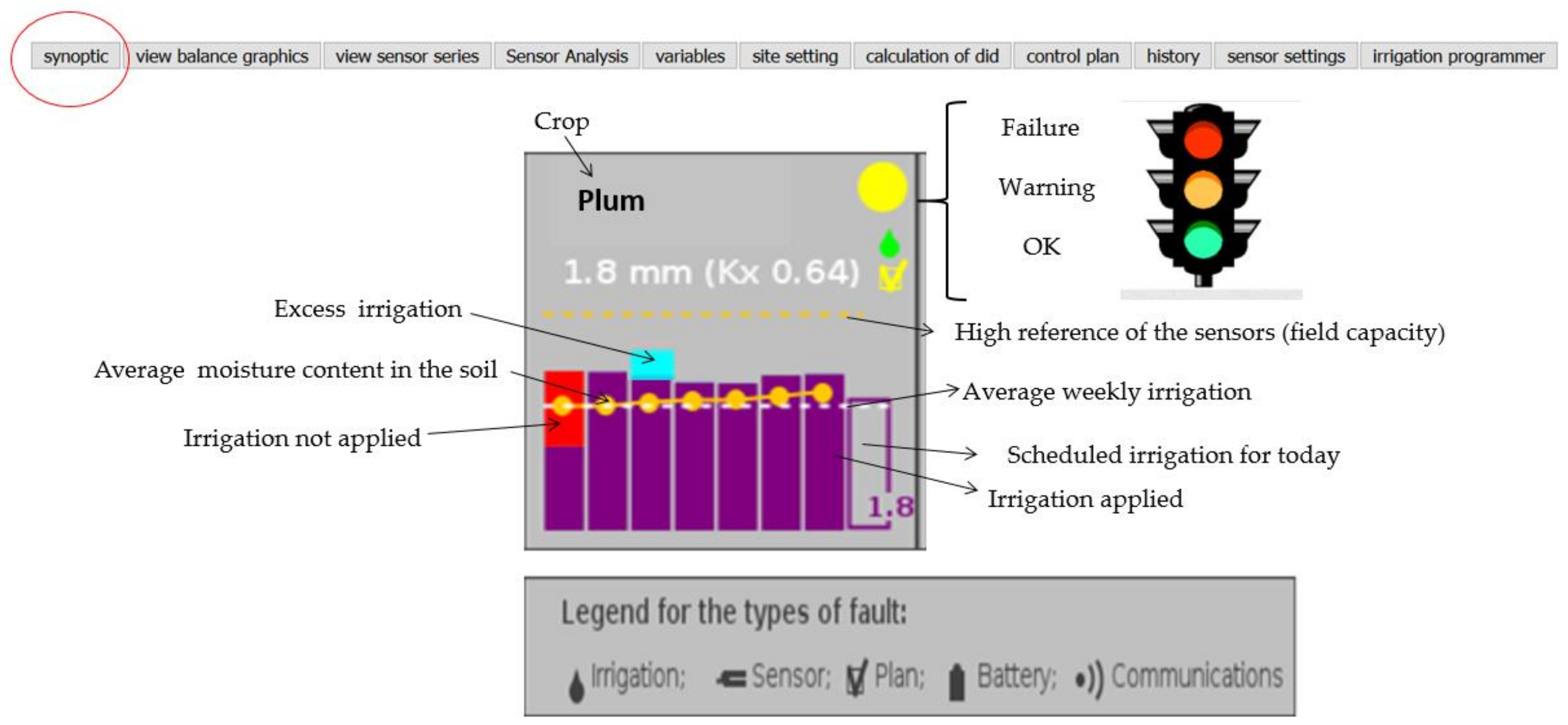
An IRRIX user interaction screenshot is shown in Figure 2. The screen shows information about the last seven days of irrigation. The traffic light system displays whether the irrigation system is operating correctly or if there has been a fault in a sensor, the irrigation system, seasonal plan, battery system, or communication system. The example in Figure 2 indicates a warning in the system due to a failure in the seasonal plan: on day one the full IRRIX-planned irrigation was not applied, and on day three an excess of irrigation water was applied.
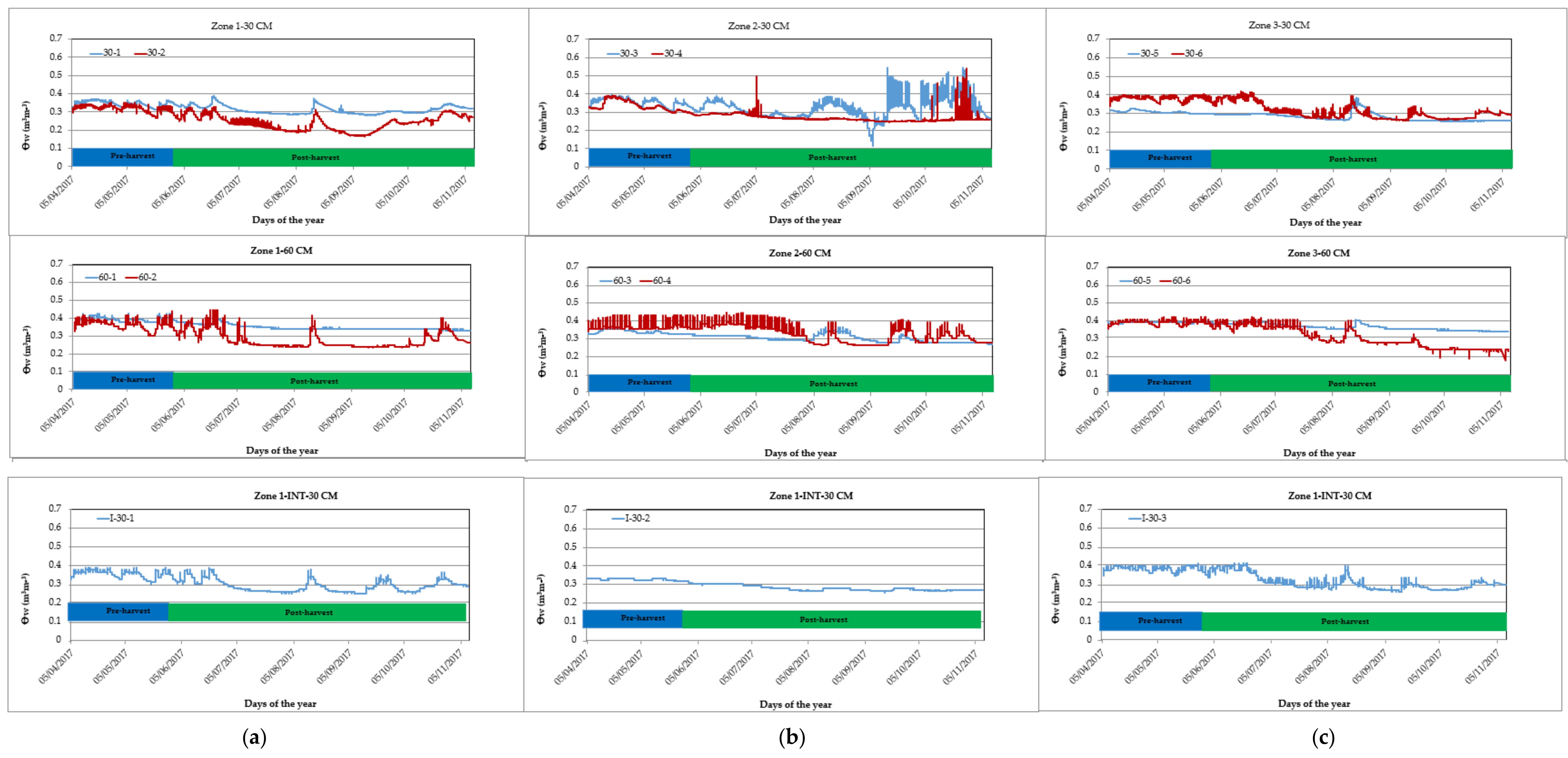
Figure 3 shows the evolution of each soil moisture sensor in the experimental plot over the course of the 2017 irrigation campaign. It can be seen that all the sensors detected changes in water content during the campaign. However, the values and seasonal evolution were different for each sensor, even when occupying the same relative position in adjacent trees or when irrigated in the same manner. An analysis of sensor-to-sensor variability is therefore required. In zone 1 (Figure 3a), the sensors situated at a depth of 30 cm were very sensitive to the irrigation, responding rapidly to it and presenting a marked amplitude response between the minimum pre-irrigation values and the maximum values on terminating the irrigation. As for the sensors situated at a depth of 60 cm, the 60-1 sensor recorded weaker irrigation-related variations than the 60-2 sensor. The sensor situated between drippers (I-30-1) responded rapidly to low irrigation inputs, as did the sensors situated below the drippers, but with a comparatively delayed reaction and with a smaller amplitude between minimum and maximum values. In zone 2 (Figure 3b), the 30 cm deep sensors displayed a different behavior to those of zone 1. This may be because these sensors only detect water in a very limited surrounding soil volume of around 1 L, which may in practice be a poor representation of what is happening in the soil as a whole. This is aggravated with the use of drip irrigation, where water distribution in the bulb tends to be irregular and differs between drippers as soil is a heterogeneous medium. Such a situation is especially complex in the case of woody crop plants when the moisture sensor is placed in the wet bulb area where more root activity is expected, entailing a degree of spatial heterogeneity [3,34]. Other reasons for sensor variability include the variability that can take place in the dielectric properties of the soil water [35] or variations in soil properties, particularly in soil apparent density or the presence of macropores. In consequence, and although the sensors record a lot of data, their interpretation can be an onerous task for the irrigator, which is considerably eased by the automatic data analysis and interpretation performed by IRRIX. It can also be seen in Figure 3 how soil moisture content decreases in the postharvest period when irrigation is reduced. This decrease is detected early in zone 1 (Figure 3a) in the sensors closest to the tree. In zone 2 (Figure 3b), the information is less clear, but in zone 3 (Figure 3c) all the sensors clearly respond to the fall in irrigation inputs, but later than in zone 1.
In our study, it is possible to observe sensor reliability in all the zones (Figure 3a–c), as when a sensor ceased to function due to some serious fault it was quickly replaced by another so that the system could calculate the weighted average of the 15 moisture sensors that were initially installed. Nonetheless, if any sensor ceased to operate and was not replaced, IRRIX would have automatically removed it from the system and would not have included it in its estimations. In our study, all sensors took a value of 1 with respect to representativeness.
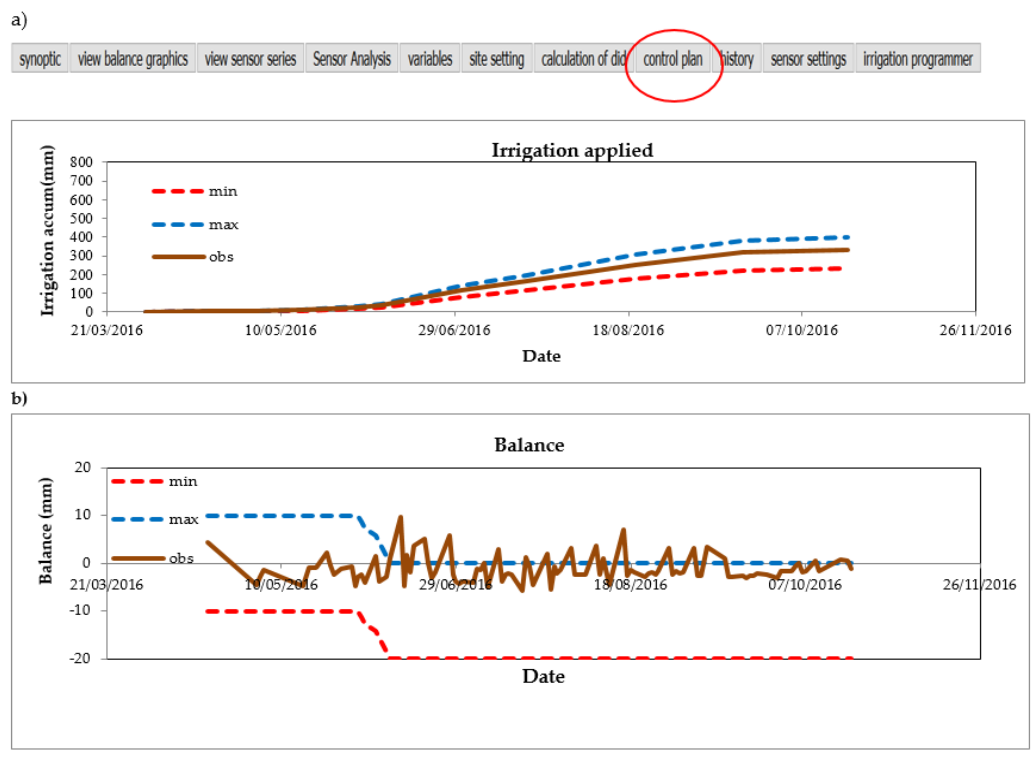
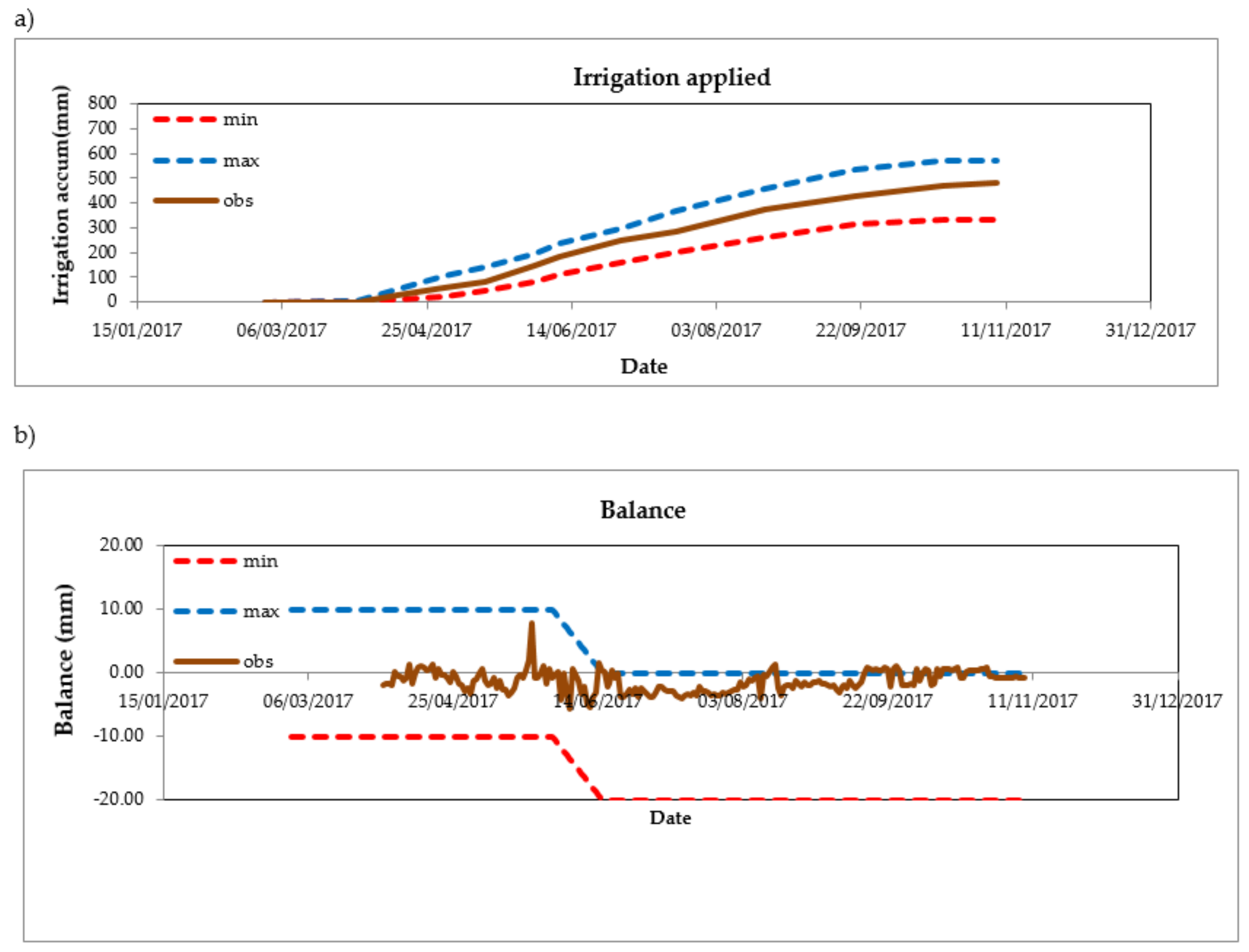
An IRRIX ‘control plan’ screenshot for the whole irrigation campaign of 2016 and 2017 is shown in Figure 4 and Figure 5, respectively. The accumulated irrigation (continuous brown line) of treatment A is shown in Figure 4a and Figure 5a, with the corresponding upper and lower bounds (red and blue broken lines) that were established in the seasonal plan. It can be seen that, in both years, the A treatment followed the established plan over the course of the campaign, remaining within the pre-established bounds. Figure 4b and Figure 5b correspond to the water balance and represent the difference between the water inputs and outputs in the soil-crop system each day (mm/day). The continuous brown line corresponds to the water balance of treatment A, and the broken lines represent the permitted maximum and minimum values in the programmed irrigation schedule. Normally, an irrigation dose is applied which maintains a balance between the inputs (rainfall and irrigation) and outputs (mainly evapotranspiration), such that the soil water balance tends to fluctuate around zero mm. However, there may be some situations in which it may be of interest to intentionally induce deviations from zero, for example, to induce a negative water balance for the application of RDI. In Figure 4b, it can be seen that RDI began on 01 June 2016, with a transition period that terminated on 10 June 2017 when the RDI treatment was fully applied. In 2017 (Figure 5b), RDI began on 30 May 2017 and full RDI application on 15 June 2017. That is, the RDI transition period was longer in 2017. It should also be noted that there were greater fluctuations in the water balance in 2016 (Figure 4b) than in 2017 (Figure 5b). This may be due to adjustments made to the system’s comfort zone after the first year.
3.2. Meteorological Conditions and Applied Water
Table 2 shows the ETo calculated using the Penman–Monteith method (ETo-PM) and the Hargreaves method (ETo-H), accumulated rainfall, mean temperature, mean air relative humidity, and preharvest and postharvest applied water for each treatment. As can be seen, the annual ETo-PM was very similar in the two years of the study, with very high values in the months of June, July, and August in both years. The ETo-H values followed the same seasonal trend as ETo-PM, though with slightly higher values in 2016 and slightly lower values in 2017. Seasonal rainfall distribution ranged between the minimum values of the summer months and the maximum values in autumn and winter of 2016 and in spring and winter of 2017. Total rainfall in the test period was 184.97 mm in 2016 and 79.2 mm in 2017, while total rainfall for the full year varied from 283.6 mm in 2017 to 525.63 mm in 2016. The difference in ETo between the two years was 82 mm according to the Penman–Monteith method but was just 38 mm according to the Hargreaves method, with a higher ETo value in 2017 than in 2016.
The amount of irrigation water was higher in 2017 as a consequence of the lower rainfall and higher ETo (Table 2). In 2016, the applied water volume in the RDI treatment was 46% less than in the C treatment, with a similar difference between the A and C treatments (45%). In 2017, water savings amounted to 38% and 41%, for the RDI and A treatments, respectively. An analysis of the water volumes applied in the different periods in each treatment shows that in the preharvest period of 2016 all three treatments received similar amounts. These volumes were very low due to the high spring rainfall. In 2017, when much higher volumes were applied, there were clear differences between treatments, with a greater volume in C and a lower volume in A. According to the pre-established irrigation scheduling criteria, the C and RDI irrigation volumes should coincide in the preharvest stage but, as a result of a breakdown, the RDI treatment received 37 mm less. However, the most significant reduction was in A, as the soil sensor feedback allowed adaptation of the irrigation doses to the available soil water content. Although in this study irrigation was initiated on the same date in all three treatments, a proposed improvement to the system would be to use the data from the sensors to determine automatically the start of the irrigation campaign. In the postharvest period, the RDI treatment received less water than the A treatment, though the difference was less in the second year as a result of the adjustments made after the first year. This water saving may also be due to the fact that the algorithm of Casadesús et al. [3] suggests that use of the water balance model allows a rapid response to changes that occur, while at the same time the feedback mechanism can adapt the amount of water to the requirements of each plot. The level of precision of the feedback mechanism is very important, and the soil water content sensors provide the precision that is required. Osroosh et al. [11] obtained similar results in water savings with respect to the control treatment.
3.3. Tree Water Status
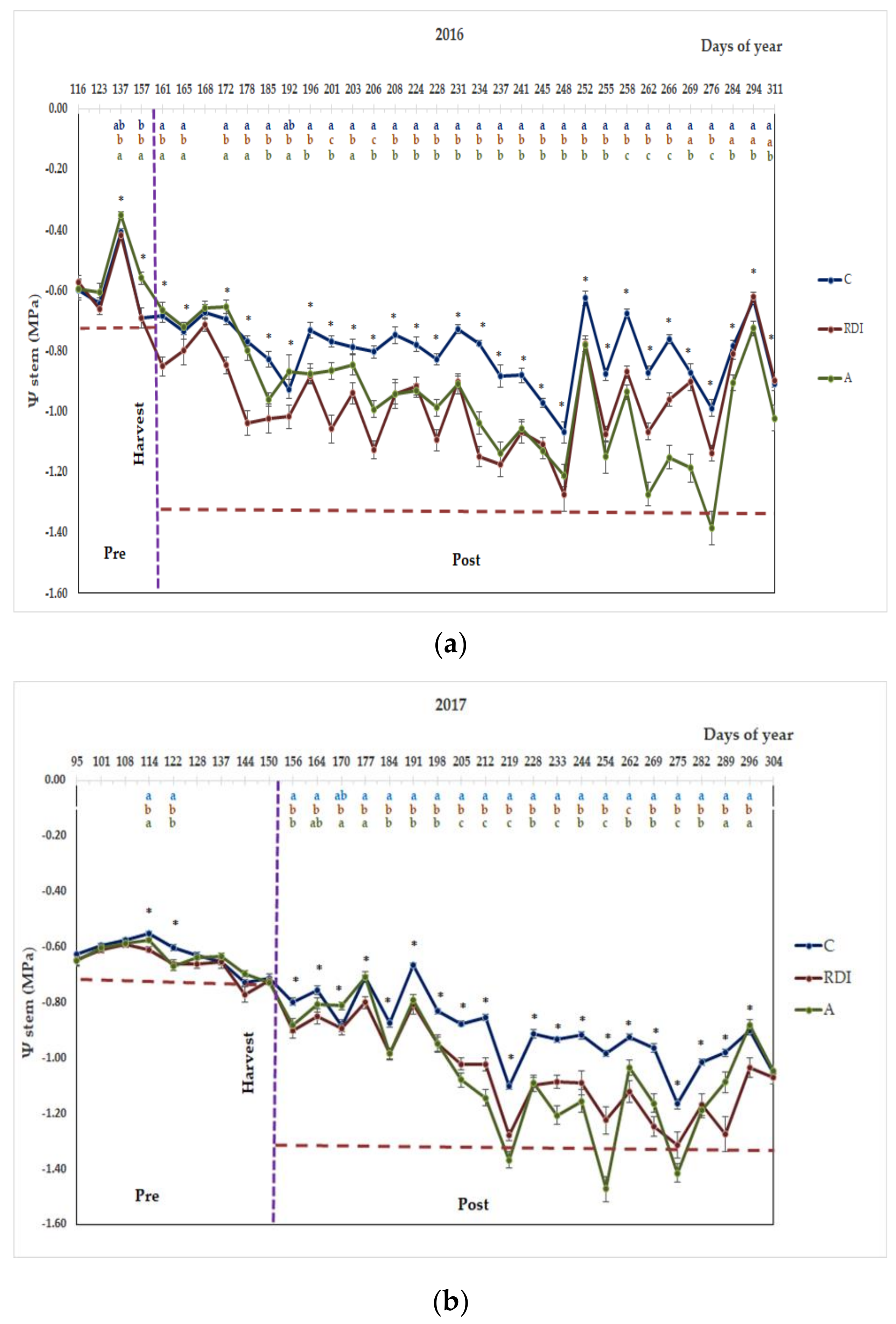
Figure 6 shows Ψstem values in 2016 (Figure 6a) and 2017 (Figure 6b). It can be seen that Ψstem decreased as the irrigation campaign progressed, even in the C treatment, though the decrease was more pronounced in the deficit treatments in the postharvest period. In 2016 (Figure 6a), Ψstem for the C treatment fell from an initial value of −0.60 MPa to a final value of −0.91 MPa. With respect to the RDI and A treatments, Ψstem fell from initial values of −0.57 MPa and −0.59 MPa, respectively, to minimum values of −1.27 MPa and −1.39 MPa, respectively, before recovering slightly before leaf fall. The A treatment had a better water status than the RDI treatment from the start of the campaign to day 208 (27 July 2016), the two treatments were similar from day 208 to day 252 (09 September 2016), and finally treatment A had a lower water status than the RDI treatment until the end of the campaign. If we consider the recommendations of Samperio et al. [21] for a late-maturing Japanese plum crop (Prunus salicina Lindl. cv. Angeleno), Ψstem should be above –0.7 MPa in stage I, –0.8 MPa in stage II, and −1.1 MPa during stage III and in the postharvest period. In our study, the Ψstem values were above −0.7 MPa in the preharvest period in the RDI and A treatments. In the postharvest period, the Ψstem values in the A and RDI treatments were above −1.3 MPa, supporting more severe stress levels but with no resulting loss in yield.
In 2017 (Figure 6b), Ψstem for the C treatment decreased from an initial value of −0.63 MPa to a final value of −1.05 MPa. In the RDI and A treatments, the initial value was −0.65 MPa and the final value −1.05 MPa. The minimum Ψstem values were −1.31 MPa and −1.47 MPa for the RDI and A treatments, respectively. In the preharvest period, significant differences can be seen between the C and RDI treatments, which may be due to the difference between the two treatments in applied water volume as a problem which occurred in the irrigation system of the RDI treatment. Differences are also observed between the C and A treatments in the preharvest period, with this worse water status possibly due to the brief reaction time in the readjustment process of the system despite the application of an appreciably lower water volume. The Ψstem range for treatment C (−0.65 MPa at the start of the campaign, −0.75 MPa before the harvest, and −1.10 MPa at the end of the campaign) is similar to the values published for well-irrigated peach [36], European plum [37], and Japanese plum [20,38,39].
3.4. Vegetative and Reproductive Growth
Table 3 shows the wood pruning results and trunk cross-sectional area increase for the different treatments. It can be seen that the results of winter pruning vary between years and type of pruned wood. The treatments which were subjected to water stress (RDI and A) have a significantly lower total pruned wood weight than the C treatment. With respect to new wood, there were significant differences between treatment C and the other treatments in both years. In 2016, and with respect to old wood, treatment A was the only one with significant differences to the other treatments. In 2017, there were no significant differences between treatments. As for summer pruning, less wood was removed in the RDI treatment than in the other treatments. Total pruned wood, considering all interventions and types of wood, was lower in the deficit treatments, with the lowest values found in the RDI treatment. It is notable that the A treatment summer pruning was similar to that of the C treatment even in the second year when less water was applied. Summer pruning could be related to tree water status (mainly after sprouting) and the reserves that the tree has of the previous year. A treatment had better water status during the preharvest of 2016 and similar Ψstem in 2017. Both aspects can explain the higher vegetative growing of A during the spring and early summer.
Deficit irrigation decreased tree vigor (ΔTCSA) compared to the C treatment in both years. There was no difference between the impact of manual and automated application of irrigation on the ΔTCSA. The RDI strategies were initially proposed to control vigor in intensive peach orchards [40]. In this case, the efficacy of the system is verified, confirming the results of Samperio et al. [20] in this same variety. Treatment A had a similar effect to the RDI treatment in both years, despite the lower RDI postharvest Ψstem value in 2016 compared to the A treatment. According to Hsiao [41], vegetative growth is highly sensitive to slight stress levels, which explains the higher new wood production and ΔTCSA in 2017 which coincided with the year of higher fruit load.
3.5. Yield and Number of Fruit/Tree
As can be seen in Table 4 the years 2016 and 2018 had remarkably higher yield than 2017. This alternation in the yield of more and less productive years is common in this cultivar and affected in a similar way to the three treatments. This natural trend in trees was accentuated in 2017 by adverse weather conditions for pollination. In 2016, there were no significant effects of irrigation on yield (Table 4). In 2017 and 2018, the deficit treatments gave a higher yield than the C treatment. These differences were due to the higher number of fruits per tree in the RDI and A treatments, though the differences were only significant in 2017 between the C and A treatments. In 2018 although A showed some tendency towards higher productions, the differences with RDI did not become significant. The RDI strategy applied in this experiment and cultivation previously demonstrated, according to Samperio et al., that it tends to increase the number of fruits per tree and therefore the tree yield [20]. In 2016, the yield results only allowed an evaluation of the capacity of the A treatment to maintain a non-detrimental preharvest water status. Given that this was a year with high rainfall, the preharvest effect of the treatments was slight. These yield results were as expected when considering that this strategy was the fruit of five years of testing RDI strategies on this cultivar [20]. Other authors, including Johnson et al. [38], obtained similar results in early-maturing plum and peach [40], where in both cases of early-maturing cultivars no significant differences in yield were obtained in the four years of the study. Naor et al. [42] reported that the risk with these strategies lies in the impact on the following campaign, which in our study was not seen in either 2017 or 2018. A second risk, described by Intrigliolo et al. [43] and Marsal et al. [44], is the accumulative effect that takes place when applying RDI strategies in several consecutive years. Intrigliolo et al. [43] detected a loss in yield in Japanese plum subjected to RDI strategies over a seven-year period, and Marsal. [44] found losses in fruit size compared to a control treatment after applying RDI for three consecutive years. In this respect, avoiding stress levels is a positive contribution, with the A treatment showing a greater ability to avoid severe stress levels than the RDI treatment in the second year of the study.
4. Conclusions
In this study, testing was undertaken using an IRRIX web platform-supported automated irrigation system. The system was evaluated for a Japanese plum crop, using a previously adapted and tested deficit irrigation strategy.
The system was able to execute the pre-established irrigation schedule without human intervention. The information captured and logged by the system in the first crop season enabled adjustments for the second crop season, demonstrating the auto-learning capacity of the system.
The automated system was able to establish an RDI strategy that avoided water stress during the more sensitive stages of the cultivar and induced moderate-to-severe stress in the less sensitive stages. The amount of manually (RDI treatment) and automatically (A treatment) applied irrigation water was similar, but not its distribution as the automated system adjusted dose amounts in accordance with the information it received from the soil moisture sensors. The yield and vigor control results obtained with the automated system were similar to those obtained by an expert in the field.
Despite the good results obtained in this study, some aspects of the system can be further improved, including the automatic assessment of the representativeness of the soil moisture sensors and the integration of a sensor that automatically characterizes the water stress of the plant.
Author Contributions
S.M. (≈40%): literature review; planning and execution of experimental work; processing of data; discussion of results and writing of paper. J.C. (≈20%): adaptation and maintenance of IRRIX and revision of the paper. C.C. (≈10%): discussion of results and final revision of the English. M.J.M. (≈10%): discussion of results. M.H.P. (≈20%): project coordinator; planning of experimental work and revision of the paper.
Funding
This research was funded by INIA (RTA2013-00045-C04 project).
Acknowledgments
The authors thank Extremadura Regional Government (GR15112, Research Group AGA001 and CCESAGROS projects).
Conflicts of Interest
The authors declare no conflict of interest.
References
- Zhu, X.; Chikangaise, P.; Shi, W.; Chen, W.; Yuan, S. Review of Intelligent Sprinkler Irrigation Technologies for Remote Autonomous System. Int. J. Agric. Biol. Eng. 2018, 11, 23–30. [Google Scholar] [CrossRef]
- Smith, M.; Pereira, L.; Berengena, J.; Itier, B.; Goussard, J.; Tollefson, L.; Van Hofwegen, P. Irrigation Scheduling: From Theory to Practice. In Proceedings of the ICID/FAO Workshop on Irrigation Scheduling, Rome, Italy, 12–13 September 1995. [Google Scholar]
- Casadesús, J.; Mata, M.; Marsal, J.; Girona, J. A General Algorithm for Automated Scheduling of Drip Irrigation in Tree Crops. Comput. Electron. Agric. 2012, 83, 11–20. [Google Scholar] [CrossRef]
- Shankar, V.; Ojha, C.; Prasad, K. Irrigation Scheduling for Maize and Indian-Mustard Based on Daily Crop Water Requirement in a Semi-Arid Region. Int. J. Civ. Environ. Eng. 2012, 6, 476–485. [Google Scholar]
- Lan, Y.; Thomson, S.J.; Huang, Y.; Hoffmann, W.C.; Zhang, H. Current Status and Future Directions of Precision Aerial Application for Site-Specific Crop Management in the USA. Comput. Electron. Agric. 2010, 74, 34–38. [Google Scholar] [CrossRef]
- Lianhao, L.; Xinyue, Z.; Xiaodong, Q.; Guiming, L. Analysis of the Decrease of Center Pivot Sprinkling System Uniformity and its Impact on Maize Yield. Int. J. Agric. Biol. Eng. 2016, 9, 108–119. [Google Scholar]
- Lin, Y.; Zhang, Z.; Xu, D.; Nie, T. Effect of Water and Fertilizer Coupling Optimization Test on Water use Efficiency of Rice in Black Soil Regions. J. Drain. Irrig. Mach. Eng. 2016, 34, 151–156. [Google Scholar]
- Duan, F.; Liu, J.; Fan, Y.; Chen, Z.; Han, Q.; Cao, H. Influential Factor Analysis of Spraying Effect of Light Hose-Fed Traveling Sprinkling System. J. Drain. Irrig. Mach. Eng. 2017, 35, 541–546. [Google Scholar]
- Kang, D.; Park, M.J.; Lee, D.H.; Rho, J.J. Mobile Services with Handset Bundling and Governmental Policies for Competitive Market. Telemat. Inform. 2017, 34, 323–337. [Google Scholar] [CrossRef]
- Romero, R.; Muriel, J.; García, I.; de La Peña, D.M. Research on Automatic Irrigation Control: State of the Art and Recent Results. Agric. Water Manag. 2012, 114, 59–66. [Google Scholar] [CrossRef]
- Osroosh, Y.; Peters, R.T.; Campbell, C.S.; Zhang, Q. Comparison of Irrigation Automation Algorithms for Drip-Irrigated Apple Trees. Comput. Electron. Agric. 2016, 128, 87–99. [Google Scholar] [CrossRef]
- Adeyemi, O.; Grove, I.; Peets, S.; Norton, T. Advanced Monitoring and Management Systems for Improving Sustainability in Precision Irrigation. Sustainability 2017, 9, 353. [Google Scholar] [CrossRef]
- Allen, R.G.; Pereira, L.S.; Raes, D.; Smith, M. Crop Evapotranspiration-Guidelines for Computing Crop Water Requirements-FAO Irrigation and Drainage Paper 56. Fao Rome 1998, 300, D05109. [Google Scholar]
- Farg, E.; Arafat, S.; El-Wahed, M.A.; El-Gindy, A. Estimation of Evapotranspiration ETc and Crop Coefficient Kc of Wheat, in South Nile Delta of Egypt using Integrated FAO-56 Approach and Remote Sensing Data. Egypt. J. Remote Sens. Space Sci. 2012, 15, 83–89. [Google Scholar] [CrossRef]
- Nolz, R.; Kammerer, G. Evaluating a Sensor Setup with Respect to Near-Surface Soil Water Monitoring and Determination of in-Situ Water Retention Functions. J. Hydrol. 2017, 549, 301–312. [Google Scholar] [CrossRef]
- Elmaloglou, S.; Soulis, K.X.; Dercas, N. Simulation of Soil Water Dynamics Under Surface Drip Irrigation from Equidistant Line Sources. Water Resour. Manag. 2013, 27, 4131–4148. [Google Scholar] [CrossRef]
- Fereres, E.; Soriano, M.A. Deficit Irrigation for Reducing Agricultural Water use. J. Exp. Bot. 2006, 58, 147–159. [Google Scholar] [CrossRef] [PubMed]
- Marsal, J.; Lopez, G.; Girona, J. Recent Advances in Regulated Deficit Irrigation (RDI) in Woody Perennials and Future Perspectives. Acta Hortic. 2008, 792, 429–439. [Google Scholar] [CrossRef]
- Costa, J.M.; Ortuño, M.F.; Chaves, M.M. Deficit Irrigation as a Strategy to Save Water: Physiology and Potential Application to Horticulture. J. Integr. Plant Biol. 2007, 49, 1421–1434. [Google Scholar] [CrossRef]
- Samperio, A.; Prieto, M.H.; Blanco-Cipollone, F.; Vivas, A.; Moñino, M.J. Effects of Post-Harvest Deficit Irrigation in ‘Red Beaut’Japanese Plum: Tree Water Status, Vegetative Growth, Fruit Yield, Quality and Economic Return. Agric. Water Manag. 2015, 150, 92–102. [Google Scholar] [CrossRef]
- Samperio, A.; Moñino, M.J.; Vivas, A.; Blanco-Cipollone, F.; Martín, A.G.; Prieto, M.H. Effect of Deficit Irrigation during Stage II and Post-Harvest on Tree Water Status, Vegetative Growth, Yield and Economic Assessment in ‘Angeleno’Japanese Plum. Agric. Water Manag. 2015, 158, 69–81. [Google Scholar] [CrossRef]
- Luthra, S.; Kaledonkar, M.; Singh, O.; Tyagi, N. Design and Development of an Auto Irrigation System. Agric. Water Manag. 1997, 33, 169–181. [Google Scholar] [CrossRef]
- Miranda, F.; Yoder, R.; Wilkerson, J.; Odhiambo, L. An Autonomous Controller for Site-Specific Management of Fixed Irrigation Systems. Comput. Electron. Agric. 2005, 48, 183–197. [Google Scholar] [CrossRef]
- Cáceres, R.; Casadesús, J.; Marfà, O. Adaptation of an Automatic Irrigation-Control Tray System for Outdoor Nurseries. Biosyst Eng. 2007, 96, 419–425. [Google Scholar] [CrossRef]
- Boutraa, T.; Akhkha, A.; Alshuaibi, A.; Atta, R. Evaluation of the Effectiveness of an Automated Irrigation System using Wheat Crops. Agric. Biol. J. N. Am. 2011, 2, 80–88. [Google Scholar] [CrossRef]
- Miller, L.; Vellidis, G.; Coolong, T. Comparing a Smartphone Irrigation Scheduling Application with Water Balance and Soil Moisture-Based Irrigation Methods: Part II—Plasticulture-Grown Watermelon. HortTechnology 2018, 28, 362–369. [Google Scholar] [CrossRef]
- Cardenas-Lailhacar, B.; Dukes, M.D.; Miller, G.L. Sensor-Based Automation of Irrigation on Bermudagrass during Dry Weather Conditions. J. Irrig. Drain. Eng. 2010, 136, 184–193. [Google Scholar] [CrossRef] [Green Version]
- Bacci, L.; Battista, P.; Rapi, B. An Integrated Method for Irrigation Scheduling of Potted Plants. Sci. Hortic. 2008, 116, 89–97. [Google Scholar] [CrossRef]
- Saab, A.; Therese, M.; Jomaa, I.; Skaf, S.; Fahed, S.; Todorovic, M. Assessment of a Smartphone Application for Real-Time Irrigation Scheduling in Mediterranean Environments. Water 2019, 11, 252. [Google Scholar] [CrossRef]
- Hargreaves, G.H. Defining and using Reference Evapotranspiration. J. Irrig. Drain. Eng. 1994, 120, 1132–1139. [Google Scholar] [CrossRef]
- Hargreaves, G.H.; Allen, R.G. History and Evaluation of Hargreaves Evapotranspiration Equation. J. Irrig. Drain. Eng. 2003, 129, 53–63. [Google Scholar] [CrossRef]
- Shackel, K.A.; Ahmadi, H.; Biasi, W.; Buchner, R.; Goldhamer, D.; Gurusinghe, S.; Hasey, J.; Kester, D.; Krueger, B.; Lampinen, B. Plant Water Status as an Index of Irrigation Need in Deciduous Fruit Trees. HortTechnology 1997, 7, 23–29. [Google Scholar] [CrossRef] [Green Version]
- Baggiolini, M. Les StadesRepérés Des ArbresFruitiers à Noyau. Rev. Romande Agric. Vitic. Arboric. 1952, 8, 3–4. [Google Scholar]
- Choi, K.; Choi, E.; Kim, I.S.; Lee, Y. Improving Water and Fertilizer use Efficiency during the Production of Strawberry in Coir Substrate Hydroponics using a FDR Sensor-Automated Irrigation System. Hortic. Environ. Biotechnol. 2016, 57, 431–439. [Google Scholar] [CrossRef]
- Kizito, F.; Campbell, C.; Campbell, G.; Cobos, D.; Teare, B.; Carter, B.; Hopmans, J. Frequency, Electrical Conductivity and Temperature Analysis of a Low-Cost Capacitance Soil Moisture Sensor. J. Hydrol. 2008, 352, 367–378. [Google Scholar] [CrossRef]
- Garnier, E.; Berger, A. Testing Water Potential in Peach Trees as an Indicator of Water Stress. J. Hortic. Sci. 1985, 60, 47–56. [Google Scholar] [CrossRef]
- McCutchan, H.; Shackel, K. Stem-Water Potential as a Sensitive Indicator of Water Stress in Prune Trees (Prunus Domestica L. Cv. French). J. Am. Soc. Hortic. Sci. 1992, 117, 607–611. [Google Scholar] [CrossRef]
- Scott Johnson, R.; Handley, D.; Day, K. Postharvest Water Stress of an Early Maturing Plum. J. Hortic. Sci. 1994, 69, 1035–1041. [Google Scholar] [CrossRef]
- Intrigliolo, D.; Castel, J. Response of Plum Trees to Deficit Irrigation Under Two Crop Levels: Tree Growth, Yield and Fruit Quality. Irrig. Sci. 2010, 28, 525–534. [Google Scholar] [CrossRef]
- Johnson, R.S.; Handley, D.; DeJong, T. Long-Term Response of Early Maturing Peach Trees to Postharvest Water Deficits. J. Am. Soc. Hortic. Sci. 1992, 117, 881–886. [Google Scholar] [CrossRef]
- Hsiao, T.C. Plant Responses to Water Stress. Annu. Rev. Plant Physiol. 1973, 24, 519–570. [Google Scholar] [CrossRef]
- Naor, A.; Peres, M.; Greenblat, Y.; Gal, Y.; Arie, B. Effects of Pre-Harvest Irrigation Regime and Crop Level on Yield, Fruit Size Distribution and Fruit Quality of Field-Grown ‘Black Amber’Japanese Plum. J. Hortic. Sci. Biotechnol. 2004, 79, 281–288. [Google Scholar] [CrossRef]
- Intrigliolo, D.; Ballester, C.; Castel, J. Carry-Over Effects of Deficit Irrigation Applied Over Seven Seasons in a Developing Japanese Plum Orchard. Agric. Water Manag. 2013, 128, 13–18. [Google Scholar] [CrossRef]
- Marsal, J.; Casadesus, J.; Lopez, G.; Mata, M.; Bellvert, J.; Girona, J. Sustainability of Regulated Deficit Irrigation in a Mid-Maturing Peach Cultivar. Irrig. Sci. 2016, 34, 201–208. [Google Scholar] [CrossRef]
Figure 1.
Components of the automatic system.

Figure 2.
Screenshot of the “synoptic” tab of IRRIX in the year 2017.

Figure 3.
Data logged from the 10HS sensors in the year 2017 in the different zones: (a) zone 1, (b) zone 2, and (c) zone 3. Θw = soil water; 30-1,30-2,30-3,30-4,30-5,30-6 are sensors installed at 15 cm from the dripper and at a depth of 30 cm; 60-1,60-2,60-3,60-4,60-5,60-6 are sensors installed 15 cm from the dripper and at a depth of 60 cm; I-30-1, I30-2, I-30-3 are sensors installed at a depth of 30 cm and located between drippers. Pre-harvest is the period from fruit set to harvest; postharvest is the period from harvest to onset of leaf fall.

Figure 4.
Screenshot of the ‘control plan’ tab of IRRIX in the year 2016, (a) the accumulated irrigation of treatment A during the irrigation campaign and (b) the water balance of treatment A during the irrigation campaign.
Figure 4.
Screenshot of the ‘control plan’ tab of IRRIX in the year 2016, (a) the accumulated irrigation of treatment A during the irrigation campaign and (b) the water balance of treatment A during the irrigation campaign.

Figure 5.
Screenshot of the ‘control plan’ tab of IRRIX in the year 2017, (a) the accumulated irrigation of treatment A during the irrigation campaign and (b) the water balance of treatment A during the irrigation campaign.
Figure 5.
Screenshot of the ‘control plan’ tab of IRRIX in the year 2017, (a) the accumulated irrigation of treatment A during the irrigation campaign and (b) the water balance of treatment A during the irrigation campaign.

Figure 6.
Seasonal variations in midday stem water potential (Ψstem) of ‘Red Beaut’ plum trees in response to different irrigation treatments during (a) 2016 and (b) 2017. Each value is the mean of 32 measurements ± standard error. Pre is the period from fruit set to harvest of the current year. Post is the period from harvest to the onset of leaf fall of the current year. The vertical dashed line indicates the moment of harvest. The horizontal dashed line indicates the threshold established for each crop phase. * Indicates significant differences according to Duncan’s multiple range test (p = 0.05). C is the control treatment and A is the automatic treatment.


Table 1.
Phenology of the crop for the different years of the study.
| Phenology | 2016 | 2017 |
|---|---|---|
| Bud burst | 27 January 2016 | 30 January 2017 |
| Flowering | 29 February 2016 | 02 March 2017 |
| Harvest | 08 June 2016 | 29 May 2017 |
| Leaf fall | 20 November 2016 | 15 November 2017 |
Table 2.
Reference evapotranspiration (ETo), rainfall, mean temperature, mean air relative humidity, and total irrigation water applied in the three irrigation treatments.
Table 2.
Reference evapotranspiration (ETo), rainfall, mean temperature, mean air relative humidity, and total irrigation water applied in the three irrigation treatments.
| Parameters | 2016 | 2017 | ||||
|---|---|---|---|---|---|---|
| Pre 1 | Post 2 | Annual 3 | Pre 1 | Post 2 | Annual 3 | |
| ETo-PM (mm) | 330.77 | 955.30 | 1286.07 | 450.06 | 918.49 | 1368.55 |
| ETo-H (mm) | 358.36 | 937.99 | 1296.35 | 420.74 | 837.52 | 1258.26 |
| Rainfall (mm) | 269.38 | 256.25 | 525.63 | 175.08 | 108.52 | 283.60 |
| T mean (°C) | 12.59 | 19.20 | 15.89 | 13.41 | 19.69 | 16.55 |
| RH mean (%) | 80.14 | 65.54 | 72.84 | 71.42 | 58.05 | 64.73 |
| Irrigation (mm) | ||||||
| C | 33 | 570 | 603 | 245 | 569 | 814 |
| RDI | 31 | 250 | 281(45.96) | 208 | 297 | 506(37.84) |
| A | 32 | 302 | 334(44.62) | 143 | 336 | 479(41.16) |
ETo-PM is the reference evapotranspiration calculated through the Penman–Monteith equation; ETo-H is the reference evapotranspiration calculated through the Hargreaves equation; RH is relative humidity; C: control; RDI: regulated deficit irrigation; A: automatic. 1 From fruit set to harvest of the current year; 2 from harvest to the onset of leaf fall of the current year; 3 from the onset of leaf fall of the previous year to the onset of leaf fall of the current year; in parentheses % savings compared to the control, calculated as: ((applied water in the control – applied water in the RDI treatment or applied water in the automatic treatment)/applied water in the control) × 100. In 2016, irrigation began on 16 April 2016 and ended on 20 October 2016. In 2017, irrigation started on 04 April 2017 and ended on 08 November 2017.
Table 3.
Effects of irrigation on annual winter pruning of new wood, winter pruning of old wood, summer pruning, total pruning, and increase in trunk cross-sectional area (ΔTCSA) for the two years of the study.
Table 3.
Effects of irrigation on annual winter pruning of new wood, winter pruning of old wood, summer pruning, total pruning, and increase in trunk cross-sectional area (ΔTCSA) for the two years of the study.
| Crop data | Treatments | 2016 | 2017 | ||
|---|---|---|---|---|---|
| C | 6.20 ± 0.35 | a | 8.68 ± 0.87 | a | |
| Winter pruning of new wood (kg/tree) | RDI | 3.84 ± 0.49 | b | 4.46 ± 0.60 | b |
| A | 4.73 ± 0.34 | b | 5.38 ± 0.58 | b | |
| Significance | * | * | |||
| C | 8.35 ± 1.51 | a | 2.53 ± 0.44 | ||
| Winter pruning of old wood (kg/tree) | RDI | 5.11 ± 1.03 | ab | 2.52 ± 0.19 | |
| A | 4.09 ± 0.65 | b | 2.27 ± 0.32 | ||
| Significance | * | n.s. | |||
| C | 11.48 ± 0.45 | a | 9.94 ± 0.42 | a | |
| Summer pruning (kg/tree) | RDI | 9.56 ± 0.78 | b | 8.43 ± 0.66 | b |
| A | 10.55 ± 0.44 | ab | 9.02 ± 0.25 | ab | |
| Significance | * | * | |||
| C | 26.04 ± 1.63 | a | 21.15 ± 1.14 | a | |
| Total pruning (kg/tree) | RDI | 18.52 ± 1.83 | b | 15.42 ± 1.19 | b |
| A | 19.38 ± 0.96 | b | 16.67 ± 0.86 | b | |
| Significance | * | * | |||
| C | 65.54 ± 3.77 | 69.59 ± 5.31 | |||
| ΔTCSA (cm2) | RDI | 55.47 ± 4.62 | 69.39 ± 10.54 | ||
| A | 59.72 ± 6.11 | 67.41 ± 5.71 | |||
| Significance | n.s. | n.s. |
ΔTCSA is the increase in the cross-sectional area of the trunk; total pruning is the sum of winter pruning (new + old wood) and summer pruning; * indicates significant differences according to Duncan’s multiple range test (p = 0.05); n.s. indicates not significant.
Table 4.
Effects of irrigation on annual yield and number of fruits per tree in 2016, 2017, and 2018.
Table 4.
Effects of irrigation on annual yield and number of fruits per tree in 2016, 2017, and 2018.
| Yield data | Treatments | 2016 | 2017 | 2018 | ||
|---|---|---|---|---|---|---|
| C | 15158 ± 2114.80 | 4076 ± 414.82 | b | 14491 ± 1090.55 | b | |
| Yield (kg/ha) | RDI | 14240 ± 2081.19 | 6229 ± 587.07 | a | 16448 ± 1538.96 | ab |
| A | 13697 ± 1652.65 | 7228 ± 818.03 | a | 19908 ± 1447.29 | a | |
| Significance | n.s. | * | * | |||
| C | 721 ± 113.62 | 130 ± 14.31 | b | 404 ± 29.08 | ||
| Number of fruit/trees | RDI | 681 ± 99.08 | 203 ± 19.21 | ab | 456 ± 50.78 | |
| A | 629 ± 88.67 | 237 ± 27.50 | a | 485 ± 34.86 | ||
| Significance | n.s. | * | n.s. |
* Indicates significant differences according to Duncan’s multiple range test (p = 0.05); n.s. indicates not significant.
© 2019 by the authors. Licensee MDPI, Basel, Switzerland. This article is an open access article distributed under the terms and conditions of the Creative Commons Attribution (CC BY) license (http://creativecommons.org/licenses/by/4.0/).
Share and Cite
MDPI and ACS Style
Millán, S.; Casadesús, J.; Campillo, C.; Moñino, M.J.; Prieto, M.H. Using Soil Moisture Sensors for Automated Irrigation Scheduling in a Plum Crop. Water 2019, 11, 2061. https://doi.org/10.3390/w11102061
AMA Style
Millán S, Casadesús J, Campillo C, Moñino MJ, Prieto MH. Using Soil Moisture Sensors for Automated Irrigation Scheduling in a Plum Crop. Water. 2019; 11(10):2061. https://doi.org/10.3390/w11102061
Chicago/Turabian StyleMillán, Sandra, Jaume Casadesús, Carlos Campillo, María José Moñino, and Maria Henar Prieto. 2019. "Using Soil Moisture Sensors for Automated Irrigation Scheduling in a Plum Crop" Water 11, no. 10: 2061. https://doi.org/10.3390/w11102061
Note that from the first issue of 2016, this journal uses article numbers instead of page numbers. See further details here.