Detecting the Response of Irrigation Water Management to Climate by Remote Sensing Monitoring of Evapotranspiration

Abstract

This study on a large irrigation scheme in Morocco addressed a two-fold question: (a) does the local water management authority adapt water releases to atmospheric water demand ET₀-P? and (b) does crop actual evapotranspiration respond to inter- and intra-annual variability in water releases? We have evaluated the inter-annual variability of ET₀-P during the period 1992–2017 and compared its anomalies (i.e., deviations from average) with anomalies in annual water release. Overall, it appeared that anomalies in water release were consistent with anomalies in ET₀-P. The actual evapotranspiration (ET_a) was estimated using a time series of multi-spectral satellite image data by applying the Surface Energy Balance (SEBAL) algorithm in a dry, wet, and reference year. We have determined the quartiles of the distribution of the ET₀-P time series to identify these three years. The dry year was 2015–2016, the wet year was 2014–2015, and the reference (median of ET₀-P) was 2013–2014. Finally, we compared seasonal and annual anomalies in ET₀-P, ET_a and release, W_d of irrigation water. In the period 1992–2017, the relative anomalies in ET₀-P and W_d were similar only in 2000–2001 and 2015–2016. The analysis of anomalies in water inflow and stocks confirmed the response in increased W_d following wet years with higher inflow and replenishment of the reservoir. The response of crop water use to the irrigation water supply was evaluated by comparing anomalies in the ratio of actual to maximum ET, i.e., ET_a/ET_c with anomalies in W_d. As regards the Sidi Bennour, Faregh, and Gharbia districts, the relative anomalies in ET_a/ET_c and W_d were consistent, i.e., they had the same sign and comparable magnitude. Overall, the study shows that water delivery W_d responds to inter-annual variability in the pre-irrigation season water inflows into the reservoirs, rather than in ET₀-P. On the other hand, actual crop water use, i.e., ET_a/ET_c, does respond to inter- and intra-annual variability in W_d. This evidence suggests that there is scope for adaptive water management based on a flexible adaptation of water release to inter- and intra-annual variability in water demand.

1. Introduction

At the present time, water resources are severely stressed and particularly scarce in arid regions of the world. In North Africa, one of the most water-scarce regions of the world, water use problems are already apparent, aquifers are over-pumped, water quality is deteriorating, and water supply and irrigation services are often rationed with consequences for human health, agricultural productivity, and the environment. The challenge is escalating as the region’s population continues to grow, as the water availability is set to fall by 50% by 2050, and if climate change affects weather and precipitation patterns as predicted, the North African region may see more frequent and severe droughts and floods [1]. Therefore, good and sustainable management of this resource is even more important.

In recent years, agricultural regions in North Africa have been subject to extensive and increasing water constraints. Climate change is projected to increase the fluctuations in precipitation and surface water supplies, which will affect the crop water requirements. These water challenges are expected to strongly impact agriculture, undermining the productivity of rain-fed and irrigated crops, and livestock activities. These changes could, in turn, further impact markets, trade, and broader food security. Irrigated agriculture remains the largest user of water accounting about 83% of annual freshwater withdrawal in North Africa [2] will be important for policymakers to focus on efforts that increase the overall efficiency of water used by the agricultural sector, reduce the sector impact on freshwater resources, and improve its resilience to water risks.

Adaptive water management is an emerging concept [3], where more emphasis is placed on variability and seasonal to annual forecast in contrast to the traditional approach of designing and operating water management systems on the basis of long-term averages and climatology. Adaptive management is a decision process that “promotes flexible decision-making that can be adjusted in the face of uncertainties; e.g., water deficit and water supply, as outcomes from management actions and other events become better understood” [4]. Adaptive irrigation water management requires seasonal to annual forecasting of, e.g., precipitation, evapotranspiration, and water demand in addition to current hydrological state variables, e.g., soil water content [5]. Although the practical implementation of adaptive irrigation water management is a very active area of research and development, the literature provides evidence of ways and means to advance in that direction.

Tanaka et al. (2006) [6] analyzed the potential of the California water supply system to adapt to long term changes in water availability and demand in relation with climate. Drieschova et al. (2008) [7] analyzed treaties governing shared international river waters to assess how the response to inter-annual variability in available water was regulated.

Interventions aiming at improving the efficiency of water use in large irrigation schemes, such as the Hetao Irrigation District in China, require accurate planning and operation of water distribution in response to the inter-annual variability in water supply and demand [8]. The rehabilitation of this irrigated area was meant to reduce water diversion from the Yellow River without reducing agricultural production. Water diversion was reduced from 768 mm in 2000 to 576 mm in 2010, while both the atmospheric water demand ET₀-P and the actual evapotranspiration (ET_a) remained rather stable and lower than ET₀, notwithstanding large inter-annual variability in water diversion.

This shows that the water management system could adapt to the reduction in water diversion by keeping constant agricultural water use (i.e., ET_a). It should be noted that water diversion was comparable with ET₀-P in 2000, and much smaller in 2010.

In Spain, river basin organizations (RBO) are responsible to develop river basin management plans (RBMP) by taking into account the expected evolution of water availability and water demand in a long period [9]. The RBMP-s are updated every five years. Within each RBO the Withdrawal Commission is responsible for the yearly adjustment of the water allocation plan in three stages from September to May. The adjustment is mainly based on current water storage in the reservoirs. In Western Morocco, our study area, the procedures to adapt water allocations to the inter-annual variability of water availability and demand are similar to the procedures applied in Spain [10]. In particular, the initial water allocations plan is adapted during the irrigation season to the evolution of climate conditions, although a combination of precipitation and storage in water reservoirs, rather than ET₀-P only, is used as an indicator of climate conditions and water availability.

From the point of view of irrigation water management, drier years are associated with larger irrigation water demand, determined by the different ET₀-P between atmospheric water demand ET₀ and precipitation (P). Alternate metrics of water deficit might be applied and are briefly reviewed below.

Zargar et al. (2011) [11] reviewed indicators of water deficit aiming at capturing the difference between precipitation and evapotranspiration. These authors highlighted the wider relevance of indicators based on precipitation and potential evapotranspiration. Tsakiris and Vangelis (2005) [12] proposed the Reconnaissance Drought Index (RDI), specifically designed to capture water deficit and defined as the ratio of the cumulative values of precipitation and potential evapotranspiration over a period of time.

The Palmer Drought Severity Index (PDSI) is very widely applied in the US and regards drought as an imbalance between water supply and water demand [13]. Zargar et al. (2011) and Vicente-Serrano et al. (2010) [11,14] proposed a new drought index combining precipitation and potential evapotranspiration into a water balance-based metric of water deficit. Zargar et al. (2011) [11] grouped indicators according to the nature of drought; particularly, they reviewed different indicators of meteorological and agricultural drought. The implementation of adaptive irrigation water management requires an indicator of crop water use to detect timely agricultural drought and an indicator of climatological water deficit to detect meteorological drought.

Accurate characterization of spatial and temporal variability of actual evapotranspiration is vital information for accurate and dynamic irrigation management [8,15]. These authors presented a detailed analysis of the seasonal and inter-annual variability of actual evapotranspiration based on Eddy-covariance (EC) observations and remote sensing retrievals, in response to precipitation and irrigation water.

The study by Zeng et al. (2010) [16] provides a good illustration of the spatial variability in ET_a in relation with hydrological processes: the highest ET_a was observed for water-bodies, wetland, and woodland where water is concentrated by surface and subsurface flow, while the lowest ET_a was observed for grasslands where precipitation was the only water source. Accordingly, the actual water deficit ET_a-P was largest for wetlands and waterbodies, thus providing a measure of water supplied by sources other than precipitation. We can, therefore, evaluate the response of irrigated lands to the inter-annual variability in water supply by analyzing the inter- and intra-annual variability in ET_a-P.

Monitoring of ET_a can be done by, e.g., EC devices, but capturing both, spatial and temporal variabilities is clearly needed for precision and adaptive irrigation water management. Very few experiments have been reported in the literature, (e.g., Li et al. (2013) [17]) where a sufficiently large number of EC devices were put in place to capture the spatial variability of actual crop water use. On the other hand, literature on studies where ET_a has been estimated, mapped, and monitored using remote sensing methods, is abundant (see e.g., Gowda et al. 2008; Li et al. 2009 [18,19]). In addition, several reviews and evaluations against in situ measurement on the accuracy of remote sensing retrievals of actual ET have been published (e.g., Hu et al. 2014 [20]).

Various models have been proposed for estimating ET with remotely sensed data over the past decades, such as SEBI [21], TSEB [22], SEBAL [23,24], S-SEBI [25], SEBS [26], LSA-SAF MSG ET [27], STSEB [28], GLEAM [29], and MODIS-ET [30]. Ruhoff et al. (2013) [31] evaluated the daily MODIS ET product against EC measurement in the Rio Grande basin: RMSE was 0.78 and 0.46 mm d⁻¹ at two different EC sites, the basin-wide mean annual ET was 21% lower than the estimate from a hydrological model. Hu et al. (2014) [20] evaluated MODIS and LSAF-SAF MSG ET data product against EC measurement at 50 locations in Europe. RMSE varied from 0.33 to 1.57 mm/d for MODIS ET and from 0.27 to 1.27 mm^−d for LSAF-SAF MSG ET_a. In summary, these models generally performed well, with the relative errors of 5–30% in comparison with ground-based flux measurements on different ecosystems around the world [8]. A detailed discussion of remote sensing-based ET_a estimation models can be can be found in Gowda et al. (2008) and Li et al. (2009) [18,19].

As regards, SEBAL [8] reported that SEBAL [23,24] gave RMSE = 0.53 mm d⁻¹ or 14.6%, while Hemakumara et al. (2003) [32] reported errors from 4% to 32% on decadic ET_a. Hofste (2014) [33] evaluated several remote sensing ET_a data products at multiple locations in the Nile basin and showed that the relative RMSE of monthly estimates was, on average, 10%.

The evidence we have reviewed above suggest an overall accuracy of monthly to seasonal ET_a data products between 5% and 10%. In particular the accuracy of SEBAL estimates of actual ET is well documented and the relative error has been reported to be around 10%. We have applied SEBAL to estimate ET_a, but we have used only anomalies in ET_a, rather than its absolute value, in our analysis. Accordingly, we have concluded that the documented accuracy of SEBAL was appropriate for our purpose and did not carry out additional experiments to validate our estimates of ET_a. More generally, we have also concluded that remote sensing retrievals of ET_a can be applied to assess the effectiveness of adaptive irrigation water management to cope with inter- and intra-annual variability of water availability and atmospheric water demand.

Previous studies, e.g., [10], in the general area of information services to support irrigation management in the Doukkala irrigation scheme in Morocco have been designed and carried out by assuming that sound irrigation water management should be based on observable indicators of water demand. Moreover, in the Doukkala irrigation water is delivered to farmers if they request it. This lea to defining the broader issue to be addressed by our study: “Does the irrigation water management system responds to irrigation water demand? If this is the case, is this response observable?”

This two-fold issue can be dealt with by addressing the two research questions (a) is water diversion in the Doukkala irrigation scheme coherent with irrigation water demand and are water diversions adapted yearly to the expected irrigation water demand? (b) Do changes in water diversion have a negative impact on water availability to crops? In principle, the inter-annual climate variability may be compensated by water management by varying water releases on the basis of the expected evaporative demand. Accordingly, we have first evaluated the intra and inter-annual variability of water release in relation with evaporative demand, taking into account (P). Then we analyzed, in detail, a dry and a wet year to assess the variability in ET_a and whether this variability was consistent with changes in water releases.

2. Study Area and Data

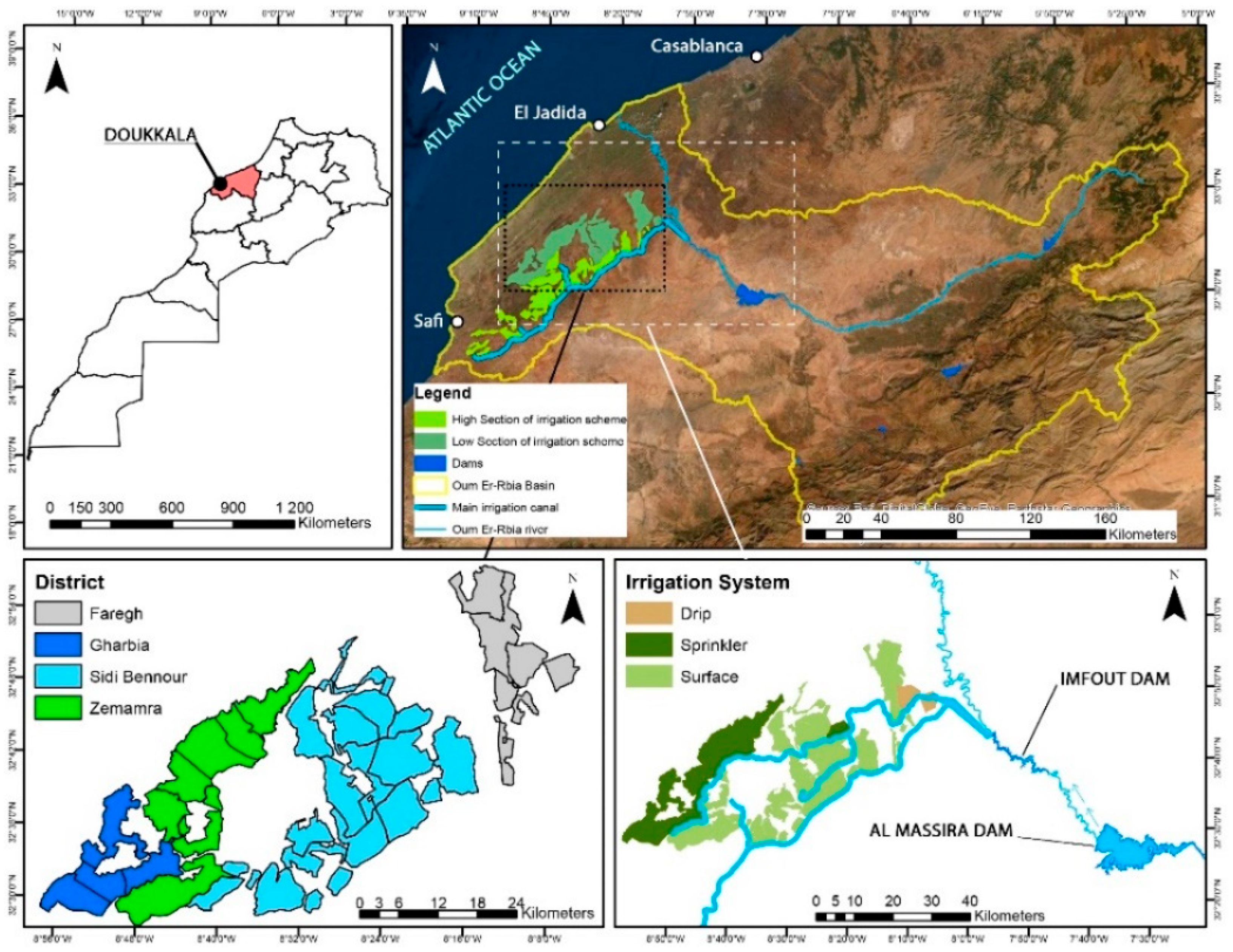
2.1. Description of the Study Area

The current study was conducted in Doukkala region which is located in Western Morocco (32°15′ N and 33°15′ N, 7°55′ W and 9°20′ W), in the downstream portion of the Oum Er-Rbia basin (Figure 1), This area includes two geomorphological units: the Doukkala and the Sahel. The plain of Doukkala covers approximatively 35,000 km². The elevation is about 120–130 m above sea level [34].

The irrigated area of Doukkala is one of the largest irrigated areas in Morocco (currently 96,000 ha), remarkable for its size and national relevance. It contributes 38% of sugar beet and 20% of commercialized milk [35]. Sugar beet, spring wheat, alfalfa (perennial crop) and summer maize are the main crops. The area is characterized by a semi-arid climate, being temperate and mild in winter and warm and dry in summer. In the period (1992–2017) mean annual rainfall was about 308 mm/year and mean annual reference evapotranspiration ET₀ about 1358 mm/year.

The Doukkala irrigation scheme includes two sub-areas: the higher section with an irrigated area of 35,000 ha and lower section with irrigated area of 61,000 ha (Figure 1). The latter includes four main districts: Faregh, Sidi Bennour, Zemamra and Gharbia, from the East to the West. Each district is divided into a number of Centers of Irrigation Management (CGRs) irrigated with different irrigation systems. The Doukkala irrigation scheme is managed by the Regional Office of Agricultural Development of Doukkala (ORMVAD) [10].

The dominant irrigation technique is surface irrigation, sprinkler irrigation is applied in a relatively large area, while drip irrigation is applied in a rather small area. According to Brouwer et al. (1989) [36], the efficiency of water application with these methods is approximately 60%, 75%, and 90%, respectively.

Sandy soils are dominant with fine and coarse texture. These soils consist of approximatively 62% of sand, 23% of clay, and 15% of silt [37].

The water resource mobilized to irrigate the Doukkala comes mainly from the Al Massira dam, one of the main water storage structures in the Oum Er-Rbia basin, with a capacity of about 2.7 × 10⁹ m³. Al Massira reservoir is one of the largest reservoirs in Morocco, with multiple uses: drinking water, agriculture, industry, and energy.

Water delivery in each rotational interval (15 days) is calculated by ORMVAD staff on the basis of current irrigated area, i.e., determined on the basis of requests by farmers for each interval. The gross irrigation water depth delivered to farmers is 864 m³/ha, equivalent to 172.8 mm/month for each hectare registered yearly with ORMVAD. This implies that the total water delivery to a farm or to a CGR, is variable in response to the requests for water by farmers. Prior to actual delivery of water, the ORMVAD technical staff in charge of each CGR carries a final check on whether the requested water volume can, and should be, delivered. This may include corrections to take into account precipitation preceding the rotational interval or short-term precipitation forecasts. In case of heavy precipitation, no irrigation water is delivered. It should be noted that this is a short-term risk-edging process, that does not evaluate a longer temporal horizon, e.g., saving irrigation water to get prepared for a drought expected later in the irrigation season.

2.2. Meteorological Data

We have used the observations of precipitation (P) and the estimates of reference crop evapotranspiration ET₀ collected by ORMVAD at the three stations indicated in the (

Table 1. Data availability at the meteorological stations in the study area; fraction is the percentage of missing observations at Zemamra replaced by observations at Metthouh and Gharbia, respectively.

Data	Meteorological Data	Meteorological Station	Fraction
From 1992 to 1996	Air temperature (Ta), Relative Humidity (RH), Wind Speed (U), Precipitations(P) and solar radiation (Rs)	Mettouh	16%
From 1996 to 2015		Zemamra	NA
From September 2015 to August 2017		Gharbia	8%

) for the period 1992–2017.

The observations at the three stations have been merged to create one continuous time series. More precisely, the observations at Gharbia and Mettouh stations were used to fill gaps in the observations at Zemamra (Table 1). In this study we took this time series as a reference for the four districts of Sidi Bennour, Zemamra, Gharbia, and Faregh (Figure 1).

In addition, the hourly data collected at the same stations for the irrigation seasons (2013–2014, 2014–2015 and 2015–2016) have been used to estimate and map (ET_a) using SEBAL (see Section 3.5). We have used hourly observations of air temperature (T_a), relative humidity (RH), wind speed (U), precipitation (R) and solar radiation (Rs) on the same dates as the satellite overpasses.

2.3. Data on Water Delivery

The water management authority (ORMVAD) collects daily data on water delivered to each CGR in the Doukkala. ORMVAD provided data for the period 1992–2017 aggregated to the entire irrigation season for each CGR. In addition, data on the water delivered to each CGR in each quarter (Figure 1) by the district water management office (Arrondissement ORMVAD) were collected for the irrigation seasons 2013–2014, 2014–2015 and 2015–2016. The irrigation season is from September to August in the following year. The selection of the three irrigation seasons is explained in Section 3.2. In this study we use the wording water delivery and the symbol (W_d) to indicate the water deliveries described in this paragraph. The data on water delivery provided by ORMVAD include a correction to account for conveyance and the distribution losses, estimated to be 35% of water allocated to irrigation at the Al Massira reservoir.

2.4. Satellite Data

All available LANDSAT-8-OLI and TIRS images for the irrigation seasons 2013–2014, 2014–2015, and 2015–2016 (see the previous Section 2.3 for additional explanations) with a nominal temporal resolution of 16 days and spatial resolution of 30m at nadir, were downloaded from https://earthexplorer.usgs.gov/. The technical specifications of the Landsat-8 data products can be found in USGS (2016) [38]. A few images were not usable due to cloud cover (see

Table 2. List of available Landsat-8 images.

Agriculture Season	Acquisition Date	DOY	Agriculture Season	Acquisition Date	DOY	Agriculture Season	Acquisition Date	DOY
2013–2014	01-Sep-13	244	2014–2015	04-Sep-14	247	2015–2016	07-Sep-15	250
	19-Oct-13	292		06-Oct-14	279		09-Oct-15	282
	04-Nov-13	308		22-Oct-14	295		10-Nov-15	314
	06-Dec-13	340		07-Nov-14	311		26-Nov-15	330
	22-Dec-13	356		09-Dec-14	343		12-Dec-15	346
	07-Jan-14	7		26-Jan-15	26		13-Jan-16	13
	08-Feb-14	39		15-Mar-15	74		01-Mar-16	60
	12-Mar-14	71		31-Mar-15	90		17-Mar-16	77
	13-Apr-14	103		02-May-15	122		18-Apr-16	108
	31-May-14	151		18-May-15	138		20-May-16	141
	16-Jun-14	167		03-Jun-15	154		05-Jun-16	157
	18-Jul-14	199		19-Jun-15	170		21-Jun-16	173
	03-Aug-14	215		05-Jul-15	186		23-Jul-16	205
	19-Aug-14	231		22-Aug-15	234		08-Aug-16	221
							24-Aug-16	237

).

All satellite images were geometrically corrected to the system of coordinates: UTM, WGS-84, zone 29 and atmospherically corrected using DOS (dark object subtraction) method [39]. For the VNIR and SWIR spectral ranges, this procedure provides at-surface spectral reflectance. The procedure applied to the TIR spectral range is described in Section 3.3.

3. Methods

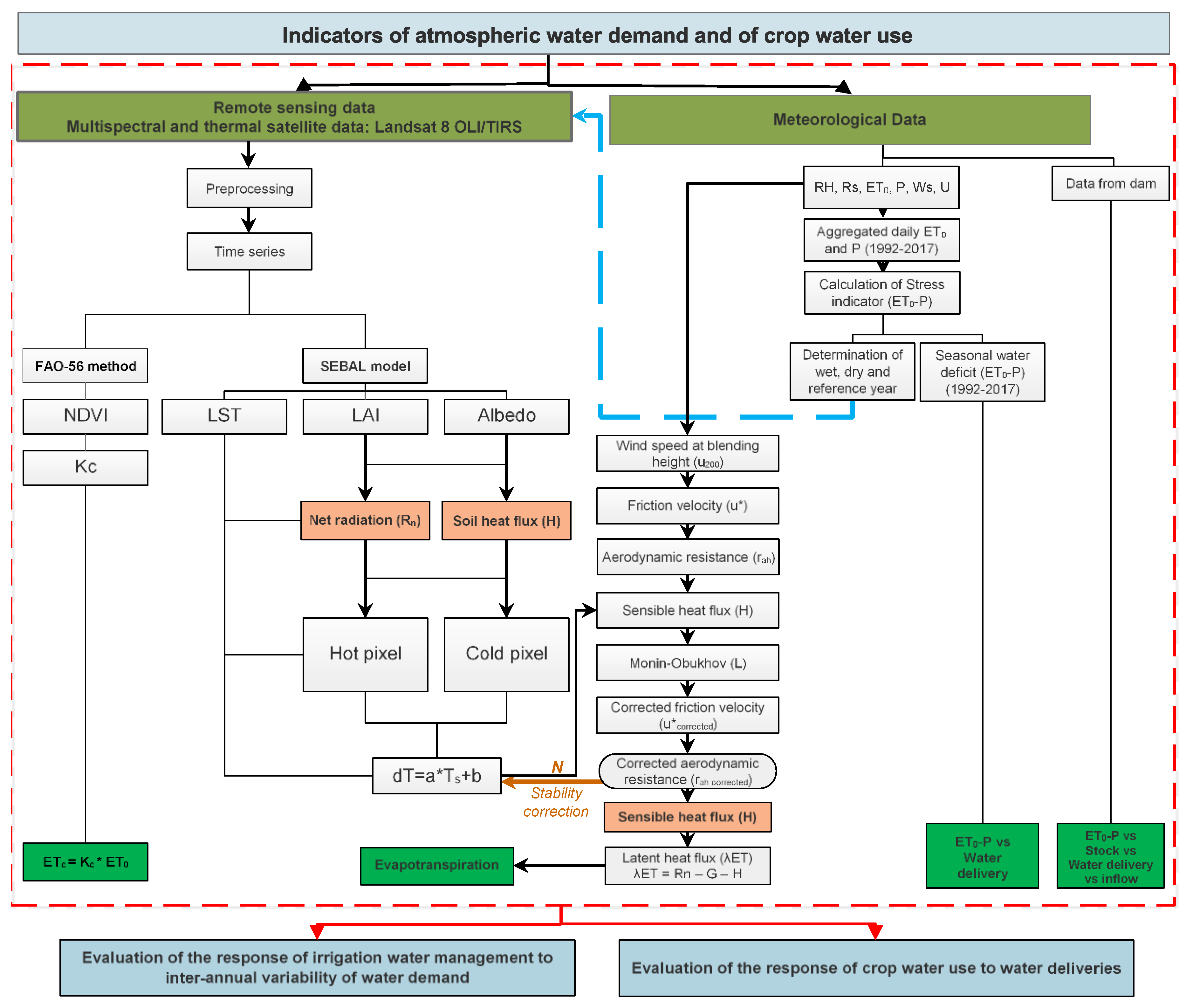
3.1. Work Flow

The approach briefly described in the introduction leads to the detailed workflow in Figure 2, which shows how the evaluation of the net atmospheric water demand relates to the detailed analysis on actual crop evapotranspiration and how the different streams of data analysis lead to the evaluation (see red arrow, Figure 2) of the response of irrigation water management to irrigation water demand and of crops to water supply. The indicators of water demand are evaluated by merging meteorological and remote sensing data (see blue arrow, Figure 2). The aerodynamic resistance, once corrected for stability is applied to determine the relationship between dT and T_s (see brown arrow, Figure 2). The elements of the workflow are described in some detail in the following sections.

3.2. Analysis of Climate Data

The first step in the work-flow described in Section 3.1 is the evaluation of the net atmospheric water demand ET₀-P. We have calculated first daily ET₀-P for each year in the period 1992–2016. The precipitation P is the time series obtained by merging available observations as described in Sect, 2 (meteorological data).

The reference crop evapotranspiration ET₀ has been calculated by applying the Penman–Monteith equation (Equation (1)) adapted from the original equation of Monteith, (1965) [40] applied to a reference crop conditions according to FAO-56 [41]:

$${\mathrm{ET}}_0=\frac{0.408\Delta ({\mathrm{R}}_{\mathrm{n}}-\mathrm{G})+\mathsf{\gamma }\frac{900}{\mathrm{T}+273}{\mathrm{u}}_2{(\mathrm{e}}_{\mathrm{s}}{-\mathrm{e}}_{\mathrm{a}})}{\Delta +\mathsf{\gamma }(1+{0.34\mathrm{u}}_2)}$$

(1)

where ET₀ = reference evapotranspiration (mm d⁻¹); R_n = net radiation at crop surface (MJ m⁻² d⁻¹); G = soil heat flux density (MJ m⁻² d⁻¹); R_n is determined by the albedo of a standard crop and G is estimated as explained in Section 3.5; γ = psychrometric constant (kPa °C⁻¹); T = mean daily air temperature at 2 m height (°C), u₂ = wind speed at 2 m height (m s⁻¹), e_s = saturation vapor pressure (kPa), e_a = Actual vapor pressure (kPa), e_s − e_a = Saturation vapor pressure deficit (kPa), Δ = slope vapor pressure curve (kPa °C⁻¹). The reference crop is assumed to have albedo = 0.23, crop height h_c = 0.12 m, and minimum canopy resistance r_c,min = 70 s m⁻¹.

The daily P and ET₀ values were aggregated to the entire irrigation season from September to August in the following year to obtain the annual net atmospheric water demand. Note that the annual values were attributed to the same year as the months January to August; see Section 3.6.1 for further details about this analysis. Next, a wet, dry and reference years were determined in this period by analyzing the frequency distribution of the annual ET₀-P. Quarterly values of ET₀-P for the wet, dry and reference years were calculated using the daily meteorological observations described in Section 2.2 over the entire irrigation season.

3.3. Preprocessing of Satellite Data

Landsat 8 LT1T products have been downloaded and processed using t ‘Preprocessing’ module of the ‘Semi-automatic classification’ plugin of QGIS [42]. Preprocessing of Landsat8 images included the following steps:

Conversion from digital numbers (DNs) to Top of Atmosphere (TOA) radiance (L_λ) is done for each VNIR and SWIR band using the band gain (ML) and offset (AL) (both present in the product metadata file).

Atmospheric correction in the VNIR and SWIR range to obtain bottom of atmosphere (BOA) radiance was performed using the revised dark object subtraction method (DOS) described by Chavez, (1996) [39]. This approach estimates the atmospheric path radiance L_p by observing dark targets in each image, i.e., by assuming that the at-satellite radiance is due to the atmosphere only. This method estimates atmospheric transmittance using a very simple parameterization evaluated by Chavez (1996) against field measurements and accurate radiative transfer models. The algorithm present in the QGIS plugin calculates L_p for each band as the difference between the maximum radiance L_min recorded among the 0.01% darkest pixels and the presumed radiance LD01% of dark objects.

In the TIR spectral range we retrieved LST by applying a four-steps procedure. In Step 1 we converted the DN-values in at-satellite radiance as done for the VNIR–SWIR spectral range. In Step 2 we converted the at-satellite Radiance into at-satellite brightness temperature using Equation (2):

$$\mathrm{T}=\frac{{\mathrm{K}}_2}{\ln (\frac{{\mathrm{K}}_1}{{\mathrm{L}}_{\mathsf{\lambda }}}+1)}$$

(2)

where T = at-satellite brightness temperature (K); L_λ = TOA spectral radiance (Watts/(m² × rad × μm)); K₁ and K₂ band-specific thermal conversion constants; values included in the metadata for each image. In Step 3, the Land Surface Emissivity is estimated from NDVI and in Step 4 LST is retrieved according to Jimenez-Munoz et al. (2014) [43] by applying the Split Window algorithm provided by Latif (2014) [44].

3.4. Estimation of Maximum Crop Evapotranspiration (ET_c)

3.4.1. General

The maximum crop evapotranspiration ET_c was estimated by the single crop coefficient approach where crop transpiration and soil evaporation are combined into a single K_c coefficient [41]:

$${\mathrm{ET}}_{\mathrm{c}}{=\mathrm{K}}_{\mathrm{c}}{\times \mathrm{ET}}_0$$

(3)

where ET₀ was estimated as described in Section 3.2.

3.4.2. Estimation of K_c Using NDVI Observations

Several authors found a good correlation between the Kc and Normalized Difference Vegetation Index [45,46], where the Normalized Difference Vegetation Index (NDVI) is defined as:

$$\mathrm{NDVI}=\frac{{\mathsf{\rho }}_{\mathrm{NIR}}-{\mathsf{\rho }}_{\mathrm{Red}}}{{\mathsf{\rho }}_{\mathrm{NIR}}+{\mathsf{\rho }}_{\mathrm{Red}}}$$

(4)

D’Urso et al. (1995), D’Urso (2001, 2010), and Calera et al. (2005) [46,47,48,49] compiled many linear relationships between K_c and NDVI to conclude that a generic, crop independent relationship could be used:

$${\mathrm{K}}_{\mathrm{c}}=1.25\times \mathrm{NDVI}+0.2$$

(5)

3.5. Retrieval of Actual Evapotranspiration ET_a: The SEBAL Model

The Surface Energy Balance Algorithm for Land (SEBAL) model, developed by Bastiaanssen (1995), Bastiaanssen et al. (1998a) and Bastiaanssen et al. (1998b) [23,24,50] accounts for bio-physical processes at the land surface and can be used to retrieve the actual evapotranspiration ET_a from multispectral imagery.

SEBAL is a single -source resistance transfer scheme based on remotely sensed data and limited weather data for deriving components of the surface energy balance equation. SEBAL computes the complete radiation and energy balance components along with the resistances for momentum, heat, and water vapor transport for each pixel [23,24]. The input data for SEBAL consists of spectral radiance in the visible, near-infrared, and thermal infrared regions of the spectrum. In addition to satellite images, the SEBAL model requires weather observations, i.e., wind speed, air humidity, solar radiation, and air temperature. Since the satellite image provides information for the overpass time only, SEBAL computes an instantaneous ET_a at the time of image acquisition. More precisely, the latent heat flux λE associated with ET_a, i.e., λET_a is calculated for each image pixel as a “residual” of the surface energy budget equation:

$$\mathsf{\lambda }\mathrm{E}={\mathrm{R}}_{\mathrm{n}}-\mathrm{G}-\mathrm{H}$$

(6)

where λE is the latent heat flux (W/m²), R_n is the net radiation flux at the surface (W/m²), H is the sensible heat flux to the air (W/m²), G is the soil heat flux (W/m²). The daily value of λE is calculated by assuming that the evaporative fraction f = (λE/ET₀), and remains constant during the day so that the daily value of λEd = EF × ET₀, d.

3.5.1. Net Radiation R_n

The net radiation R_n is obtained from the surface radiation balance, i.e., as the difference of outgoing and incoming radiant fluxes. The surface radiation balance equation was applied as described by [51].

3.5.2. Soil Heat Flux (G)

Soil heat flux is the rate of heat energy transferred from the earth’s surface to the subsurface. It is calculated as an empirical fraction of the net radiation using surface temperature (T_s), surface Albedo (α) and NDVI [52]:

$$\frac{\mathrm{G}}{{\mathrm{R}}_{\mathrm{n}}}=\frac{{\mathrm{T}}_{\mathrm{s}}}{\mathsf{\alpha }(0.0038\mathsf{\alpha }+{0.0074\mathsf{\alpha }}^2)(1-{0.98\mathrm{NDVI}}^4)}$$

(7)

If the NDVI < 0, we assume that the observed target is water and for this condition we applied G/R_n = 0.5

3.5.3. Sensible Heat Flux (H)

Sensible heat flux is the heat loss to the air by conduction and convection due to a temperature difference. The sensible heat flux is computed as:

$$\mathrm{H}=\frac{(\mathsf{\rho }\times \mathrm{cp}\times \mathrm{dT})}{{\mathrm{r}}_{\mathrm{ah}}}$$

(8)

where ρ is the air density (kg/m³), cp is the specific heat of air at constant pressure (J/kg K), dT (K) is the vertical near-surface temperature difference, and r_ah is the aerodynamic resistance to heat transport (s/m). The sensible heat flux (H) is, therefore, a function of the temperature gradient, surface roughness, and wind speed.

There are two unknowns in Equation (8), r_ah and dT, to be estimated. dT represents a temperature difference (T₁ − T₂) between two heights (z₁ and z₂). This temperature difference is used because satellites measure radiometric temperature which can differ from aerodynamic temperature by several degrees [53]. It is assumed that a linear relationship exists between dT and T_s:

$${\mathrm{dT}=\mathrm{b}+\mathrm{aT}}_{\mathrm{s}}$$

(9)

This is a key element of the entire SEBAL approach, since this linear relationship is applied in a self-calibration procedure as explained below.

The coefficients a and b in Equation (9) are determined by fitting this linear relationship to two reference values of dT assumed to apply at the surface temperature of reference hot/dry and cold/wet targets, to be selected within the observed scene. Ideally H_cold = dT_cold = 0 at the surface temperature of the Cold/Wet target and Hhot = R_n − G, dT = dT_hot at the surface temperature of the hot/dry target. The selection of the cold and hot reference targets is critical to the accuracy and reliability of the SEBAL estimates of ET_a, especially when time series of ET_a are being generated.

The selection of the cold/wet and hot/dry reference targets has been done in different ways in SEBAL applications reported in literature. In this study we have selected “cold” pixels by sampling water bodies where H_cold = dT_cold = 0. The water bodies are identified by a water mask generated beforehand by using a multi-spectral satellite image at high spatial resolution. On these pixels, the surface energy balance equation is of the form: R_n = G + λET. The “hot” reference targets are identified by selecting the pixels in the upper 20% tail of the T_s distribution in each image. The “hot” reference temperature is estimated by calculating the average of pixels selected in this way. In the “hot” pixels we assume that there is no latent heat flux, i.e., λET = 0 and H = R_n − G.

Temporal integration of instantaneous ET_a values: Our objective is to estimate actual crop water use over a long period of time, i.e., we need to estimate quarterly and seasonal ET_a. This requires a two-step temporal integration of the instantaneous ET_a estimated as described above.

The integration of instantaneous to daily ET_a is done by assuming that the evaporative fraction f = ET_a/ET₀ remains constant during daytime or at least during the central hours of the day when the contribution to daily ET_a is largest. With regard to the period in-between two sub-sequent image acquisitions, the same assumption f = const is applied to obtain the daily ET_a values from daily ET₀ and finally the daily ET_a is added up to obtain the required quarterly and seasonal ET_a.

3.6. Evaluation of the Response of Water Management to Water Demand and Impact on Crop Water Use

3.6.1. Evaluation of the Response of Irrigation Water Management to Inter-Annual Variability of Atmospheric Water Demand

For the period 1992–2017 and for the entire Doukkala irrigation scheme, we calculated the anomalies, i.e., the deviations from average, of ET₀-P and of the water deliveries (see Section 2.3) to assess whether the water management system responds to water demand by adjusting water deliveries. To compare with ET₀-P, expressed in mm for the entire irrigation season, the total water delivery to the entire Doukkala was divided by the total irrigated area, as determined by ORMVAD, to obtain water delivery in mm for the entire irrigation season. It should be noted that the total irrigated area was 61,000 ha from 1992–1993 to 2000–2001, when the higher Section (see Section 2.1) became fully operational, and 96,000 ha after that, i.e., from 2001–2002 to 2016–2017. The data on water delivery is normally collected by CGR (see Section 2.3), while ORMVAD provided the aggregated values described above for this study.

For the years 2013–2014, 2014–2015, and 2015–2016, ORMVAD provided the data on water deliveries disaggregated by quarter and by CGR, along with the corresponding irrigated area. The quarterly data on volumetric water delivery was divided by the irrigated area to obtain the quarterly water deliveries in mm for each CGR.

The response of the water management system to water shortages was evaluated with both data sets by comparing both absolute and relative anomalies in ET₀-P and water delivery. The comparison was done by evaluating both the timing and the correlation of such anomalies.

3.6.2. Evaluation of the Response of Crop Water Use to Water Delivery

Given the observed inter-annual and intra-annual (inter-quarter) variability in water deliveries and ET₀-P, we have evaluated the impact of this variability on actual crop water use, as captured by the ET_a maps, generated by applying the SEBAL procedure (see Section 3.5).

On the basis of the analysis described in Section 3.6.1, we have identified (see Section 4.1) in the period 1992–2017 a dry year, i.e., the largest ET₀-P, a wet year, i.e., the smallest ET₀-P, and a reference year, i.e., the median ET₀-P. The availability of satellite data restricted this analysis to the years 2013–2014 (reference), 2014–2015 (wet), and 2015–2016 (dry) (see Section 2.4).

We have applied two indicators of crop water use, i.e., ET_a and the ratio ET_a/ET_c, and compared the absolute and relative anomalies in both indicators with the anomalies in water deliveries.

4. Results

4.1. Analysis of Climate Data

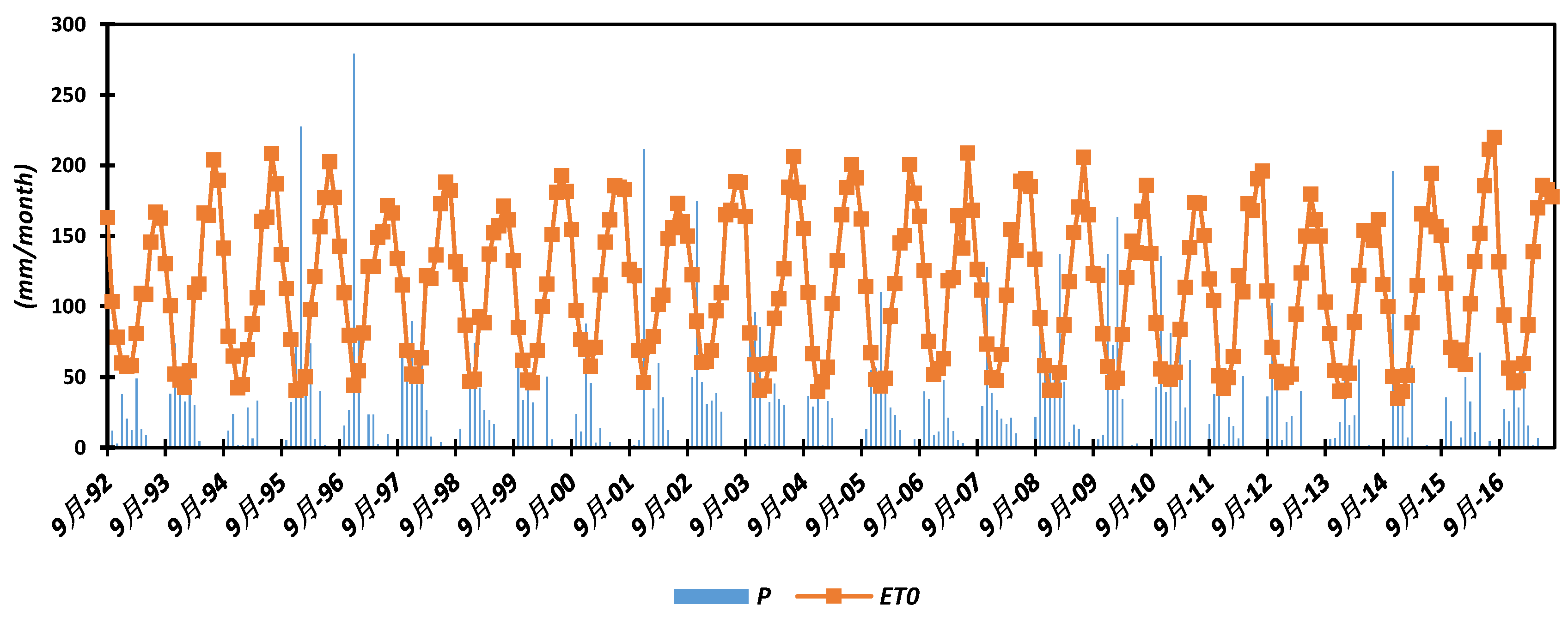
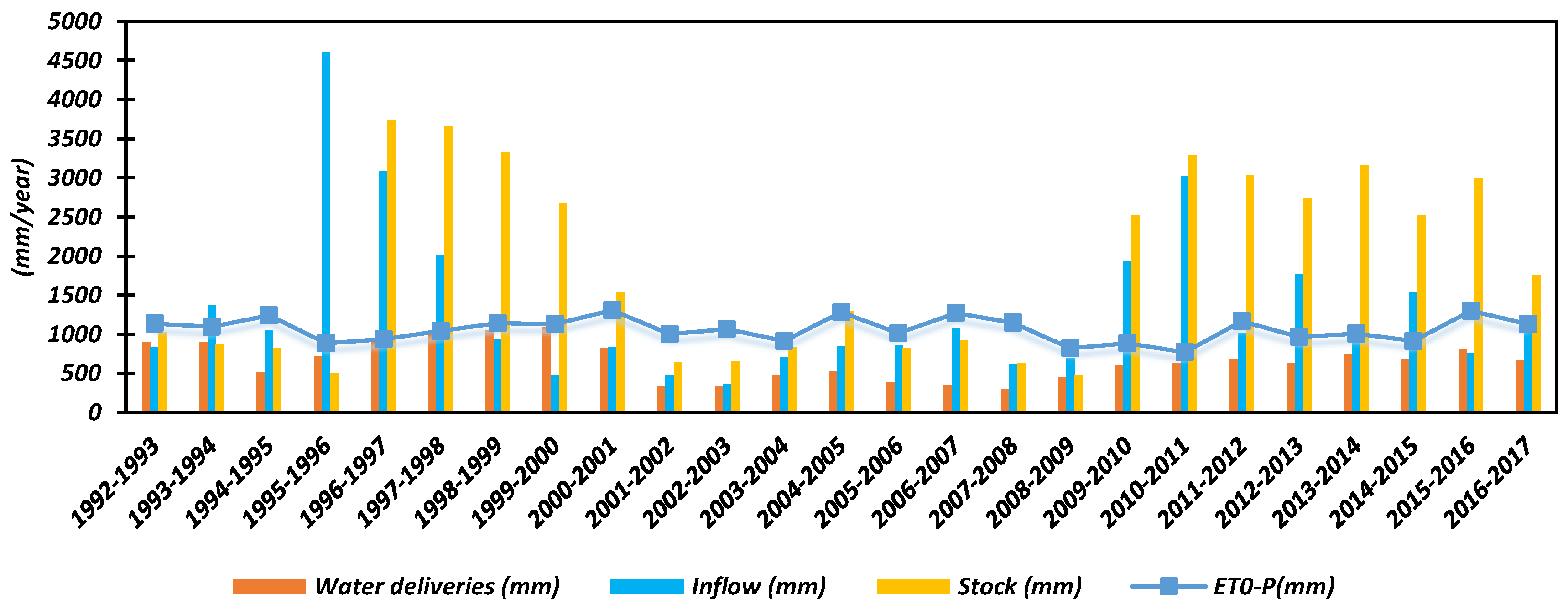
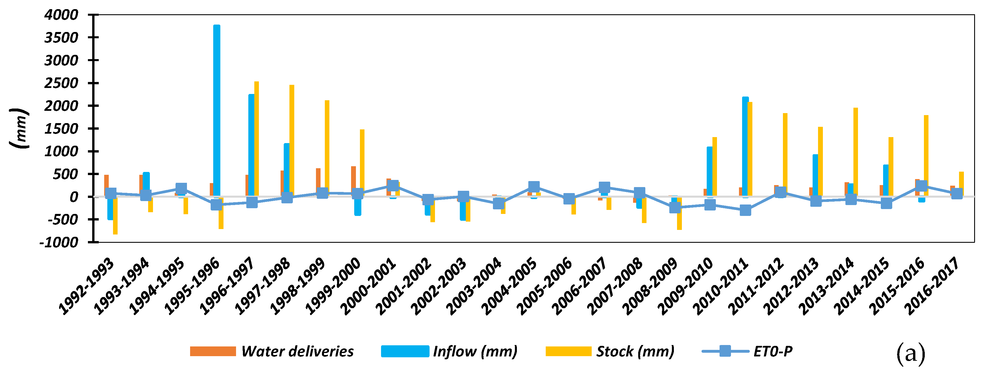
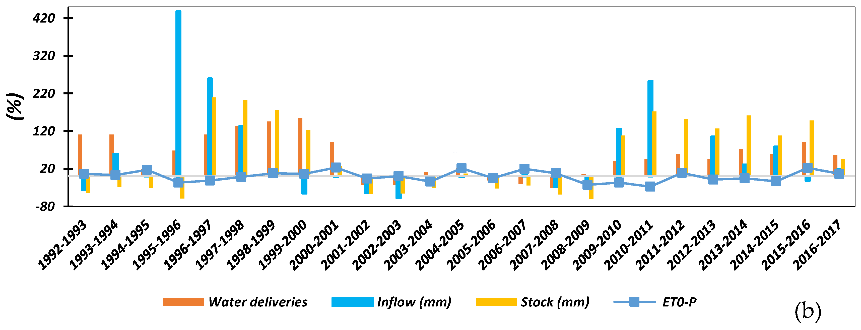
4.1.1. Inter-Annual Variability 1992–2017

The region of Doukkala is characterized within a year by clearly separated dry, i.e., with ET₀ ≫ P, and wet, i.e., with ET₀ ≅ P periods (Figure 3). In addition, the inter-annual variability of precipitation is rather large, while is relatively low in ET₀ (Figure 3). Extreme hydrometeorological events are not rare in the autumn and winter, e.g., 279 mm in December 1996 and 196 mm in November 2014. The high values of summer ET₀, however, lead to a very large intra-annual variability of ET₀-P. This led us to investigate in detail the possible response of W_d to both the inter and intra-annual variability of ET₀-P.

We have evaluated ET₀-P as an indicator of atmospheric water demand (see Section 3.2). It should be noted that W_d was rather stable and around 482 mm year⁻¹ in the period 2013–2016. In earlier years the inter-annual variability is rather large in both ET₀-P and W_d (Figure 4). The former varies between a minimum of 767.5 mm year⁻¹ and a maximum of 1305.8 mm year⁻¹. The latter, between a minimum of 191.6 mm year⁻¹ and a maximum of 708.6 mm year⁻¹. Overall, W_d is much smaller than ET₀-P and there is no evident correlation between ET₀-P and W_d. The reservoir water balance followed approximately the rule:

$${\mathrm{stock}(\mathrm{year}}^{+1}{)=\mathrm{stock}(\mathrm{year})+\mathrm{inflows}(\mathrm{year})-\mathrm{W}}_{\mathrm{d}}(\mathrm{year})-\mathrm{reservoir}\mathrm{evaporation}(\mathrm{year})$$

(10)

This equation is approximate since it does not include other water users besides the Doukkala irrigation scheme.

The exceptionally high precipitation in the year 1995–1996 led to a sharp increase in the inflow into the water reservoir of Al Massira and to its replenishment with a delay of approximately one year. W_d increased gradually as the reservoir filled up. Following the dry period of 2001–2009, during which water inflow, stock and W_d were quite consistent, a wet period followed, and the reservoir filled up at the same time as the inflow increased. In the same period the W_d remained rather constant, i.e., the improved water availability did not lead to higher W_d, although the latter remained much lower than ET₀-P. It should be recalled that that the Higher Section (35,000 ha) became fully operational in the irrigation season 2001–2002, thus raising new challenges in the equitable allocation of available irrigation water.

Likewise, the annual anomalies in W_d were not well correlated with ET₀-P (Figure 5). The absolute anomalies (Figure 5a) do not suggest a clear response of W_d to evaporative demand. In the period 1992–2017, the relative anomalies in ET₀-P and W_d (Figure 5b) were rather similar only in 2000–2001 and 2015–2016. On the other hand, there were 11 years when these relative anomalies had the same sign, i.e., both positive or negative, although different in magnitude. Moreover, the relation between absolute (Figure 5a) and relative (Figure 5b) anomalies was quite different for the years past 2010.

The analysis of anomalies in water inflow and stocks confirms the response in increased W_d following wet years with higher inflow and replenishment of the reservoir. The time lag between changes in water stock and water inflow was approximately one year from 1995–1996 (peak inflow) to 1996–1997 (maximum water stock) while it took two years to reach the maximum W_d in 1999–2000. This delay seems determined by the reservoir operation, but it was beneficial since ET₀-P was much larger than average in 2000–2001. In the extended dry period 2001–2009 the reduction in W_d was mitigated by exploiting the water stored in the preceding wet years, but anomalies in W_d remained negative for the entire period. The increase in water inflow in 2009–2010 allowed to replenish the water stock depleted during the dry years, but W_d was kept rather constant and close to the average. The latter was consistent with ET₀-P slightly fluctuating around the average except in 2015–2016 when ET₀-P was significantly larger than average and a large fraction of the water stock was depleted to increase W_d (Figure 5a,b).

4.1.2. Selection of Dry, Wet, and Reference Years

To identify the dry, wet, and reference years (see Section 3.2) we have used the 25 yearly values (Figure 3) of ET₀ and P provided by ORMVAD, where ET₀ was estimated according to FAO 56 [41], as detailed in Section 3.2. Next, we have determined the quartiles of the distribution of ET₀-P (

Table 3. Potential annual water deficit ET₀-P 1992–2016: inter-quartile ranges.

Quartile	ET0-P (mm year−1)
Minimum	767.5
Q1 (25%)	936.1
Q2 (50%)	1065.2
Q3 (75%)	1145.7
Maximum	1305.8

). By crossing the years for which the high-resolution satellite data are available with this distribution, we see that the year 2015–2016 falls between Q3 and the maximum, i.e., the range of highest atmospheric water demand, the year 2014–2015 between the minimum and Q1, i.e., the range of lowest water deficit. The ET₀-P in the year 2013–2014, i.e., 1005 mm year⁻¹, is slightly lower than the median ET₀-P, i.e., 1042 mm year⁻¹, thus we took 2013-2014 as a reference year. ET₀-P was 914 mm year⁻¹ in 2014–2015 and 1296 mm year⁻¹ in 2015–2016.

We can then conclude that the years for which satellite data are available to fit well our objective, notwithstanding the limitations due to the available satellite datasets.

4.1.3. Intra-Annual Variability

Assuming that any difference in W_d in relation with ET₀-P would be more evident when comparing hydrologically different years, we focused our analysis of intra-annual variability on the dry, reference and wet years described above. To evaluate whether quarterly W_d is determined to guarantee adequate water supply through the yearly sequence of low and high-water deficit periods, we have compared quarterly values of anomalies in ET₀-P and W_d for each district of the Doukkala irrigation scheme (Figure 6). The anomalies are the deviations from the mean water delivery over all quarters and years, calculated separately for each district. Overall, the anomalies in W_d are much smaller than the anomalies in ET₀-P, although higher than average W_d coincides with higher than average ET₀-P. The latter suggests that the water management authority aims to increase W_d when evaporative demand is larger, although the increase in water delivery is much smaller than the increase in evaporative demand. This feature applies to all districts although it is less evident in the case of Zemamra. To interpret the results in Figure 6 it should be taken into account that the annual W_d in the years 2013–2016 was rather stable (Section 4.1.1 and Figure 4). It should also be taken into account that the quarterly values shown in Figure 6 relate to the sequence of the reference, wet and dry years. It should be noted that water deliveries in the 3rd quarter are slightly higher than average, if at all, although the atmospheric water demand in the same quarter is always much larger than average (i.e., large positive absolute anomalies).

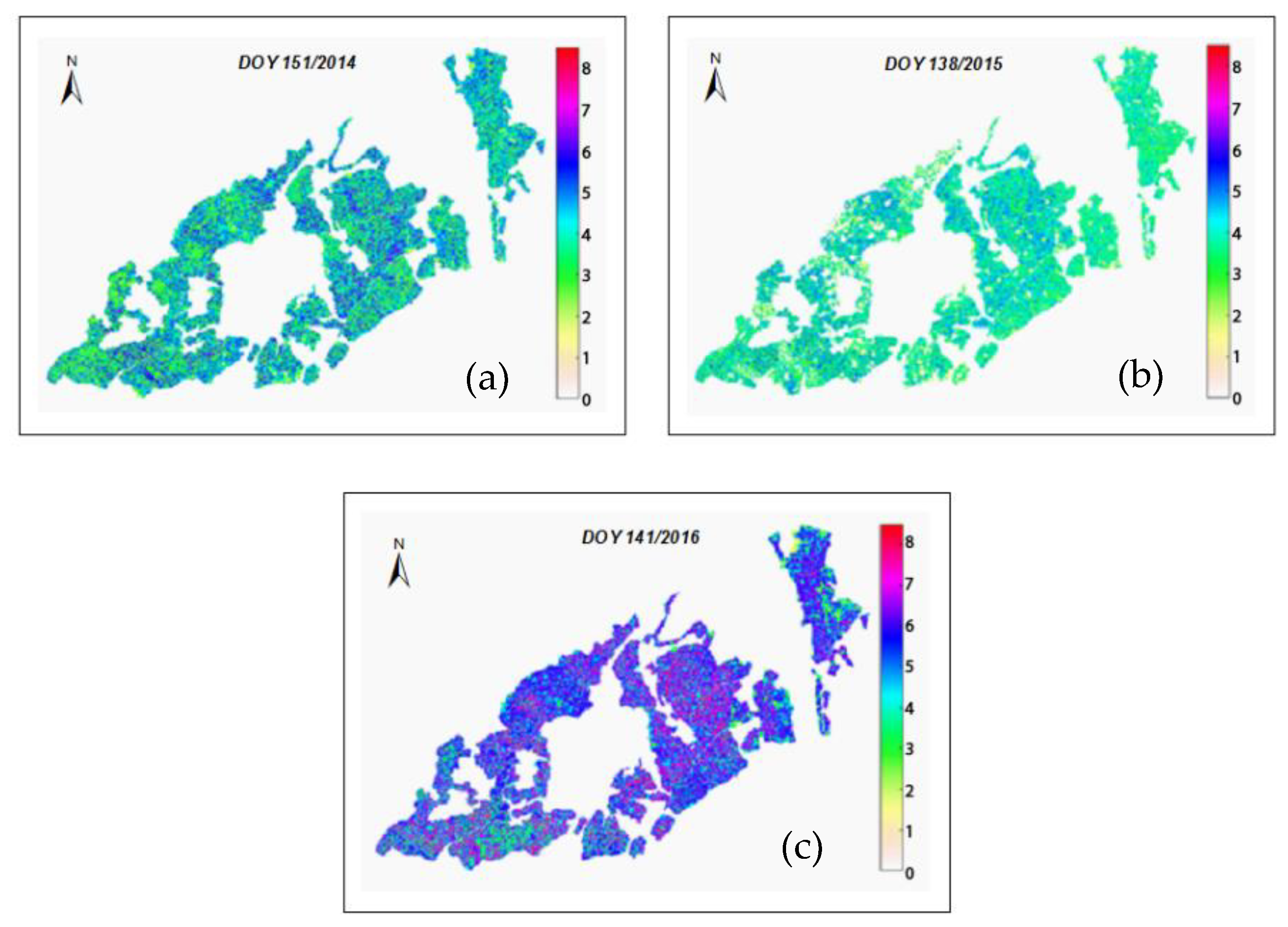
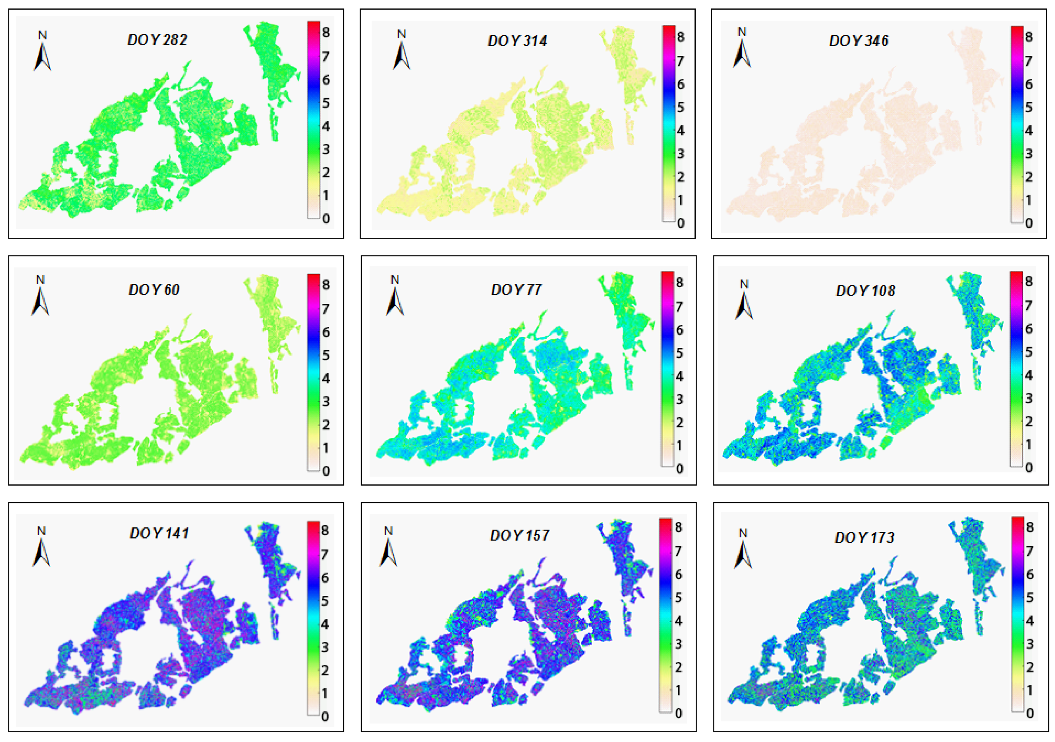
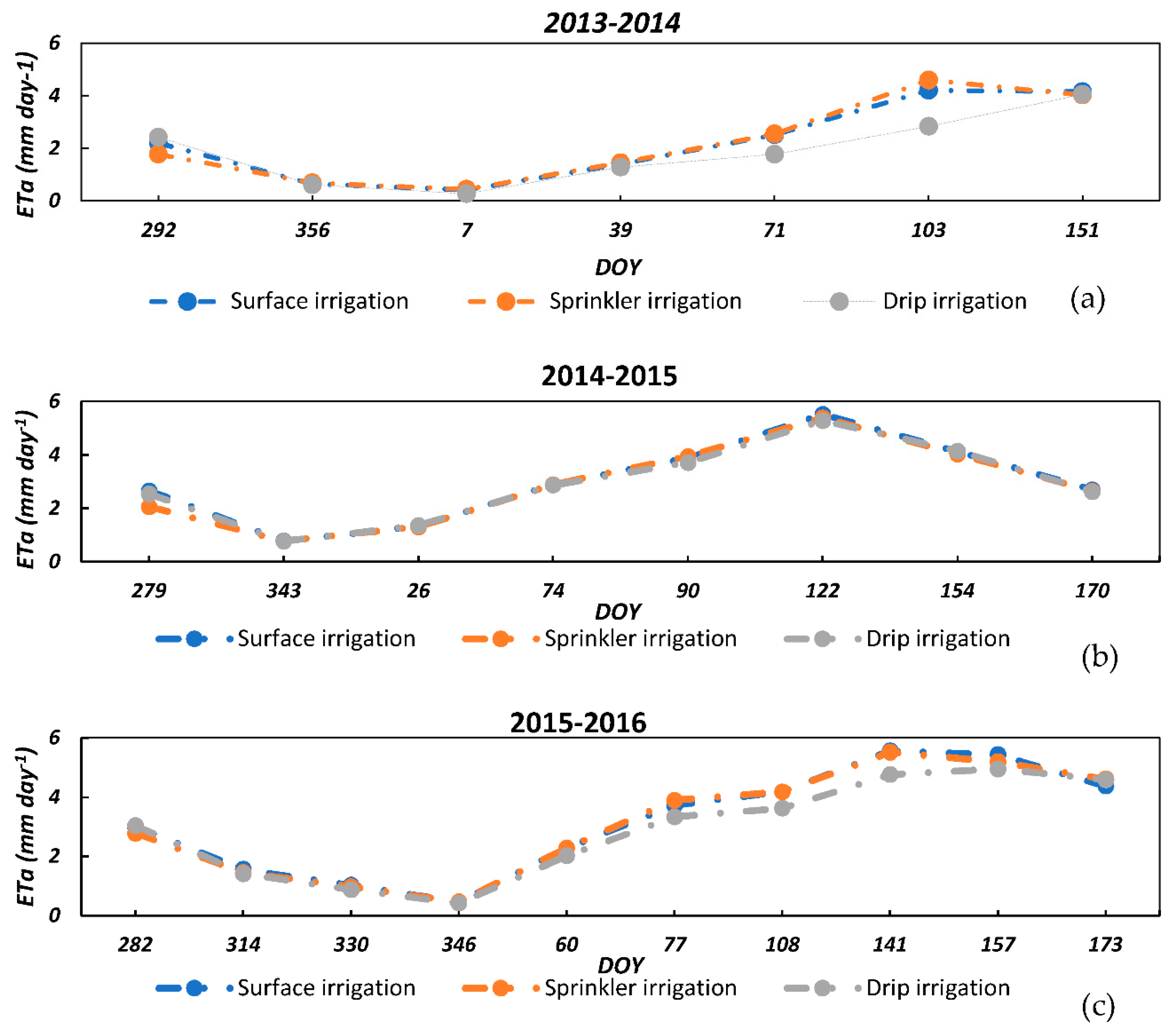
4.2. Mapping and Monitoring of Crop Water Use

As explained above we have calculated and mapped ET_a for the three selected years. The results obtained for late-spring and summer (Figure 7) are consistent with the expected impact of the dry, wet and average conditions in the three years. The highest ET_a values were observed in the year with the highest atmospheric water demand, i.e., the dry year 2015–2016. The lowest ET_a values in the year with the lowest atmospheric water demand, i.e., the wet year 2014–2015, while ET_a values in-between these two extremes were observed in the reference year 2013–2014. In addition, the spatial variability of ET_a was largest in May 2015–2016. This leads to a hypothesis, i.e., that water supply meets actual water requirements in all conditions and ET_a increases in response to the ET₀-P.

The evolution through the year 2015–2016 (Figure 8) reflect the expected seasonality, but the higher ET₀, which characterized this year lead to a larger winter-summer difference in ET_a. Likewise, the drier conditions in 2015–2016 led to a larger spatial variability in ET_a in spring and summer. Differences up to 6 mm d⁻¹ can be noticed in ET_a on DoY 157, which suggest large differences in the distribution and use of irrigation water, these results clearly require detailed data on water delivery to and within the areas served by tertiary canals for a better understanding of irrigation water management in the Doukkala.

Although no detailed data are available on the irrigation system applied in each parcel, some CGRs are dominated by surface irrigation, others by sprinkler and very few by drip irrigation. It is, therefore, possible to extract samples of the ET_a time series of maps, e.g., as in Figure 8, and average the ET_a values over the CGRs stratified by irrigation system. This was done separately for the reference, wet, and dry years (Figure 9). ET_a remains rather similar in areas dominated by surface and sprinkler irrigation, regardless of the season and the year. On the contrary, ET_a was clearly lower in areas dominated by drip irrigation in both the reference and the dry year (Figure 9), while no difference was observed in the wet year. Moreover, this difference appears earlier in the dry year, which clearly suggests a better control of water supply by drip irrigation, where water is supplied to match crop transpiration, while limiting soil evaporation. In the wet season, the soil surface remains wet because of precipitation and the evaporation remains high under both surface/sprinkler and drip irrigation. In the dry period in the plots with drip irrigation the soil surface dries out and evaporation becomes rather small. Under these conditions the sum of evaporation and transpiration tends to be lower under drip irrigation than under surface or sprinkler irrigation.

4.3. Response of Relative Evapotranspiration to Irrigation Water

As explained in Section 3.6.2 we have evaluated crop response to irrigation under varying climate forcing as measured by ET₀-P and we have applied changes in the ratio ET_a/ET_c as a measure of response. In a similar way as done earlier (see Figure 5) to evaluate anomalies in W_d, we have evaluated relative anomalies in ET_a/ET_c. This evaluation has been done separately for each irrigation district.

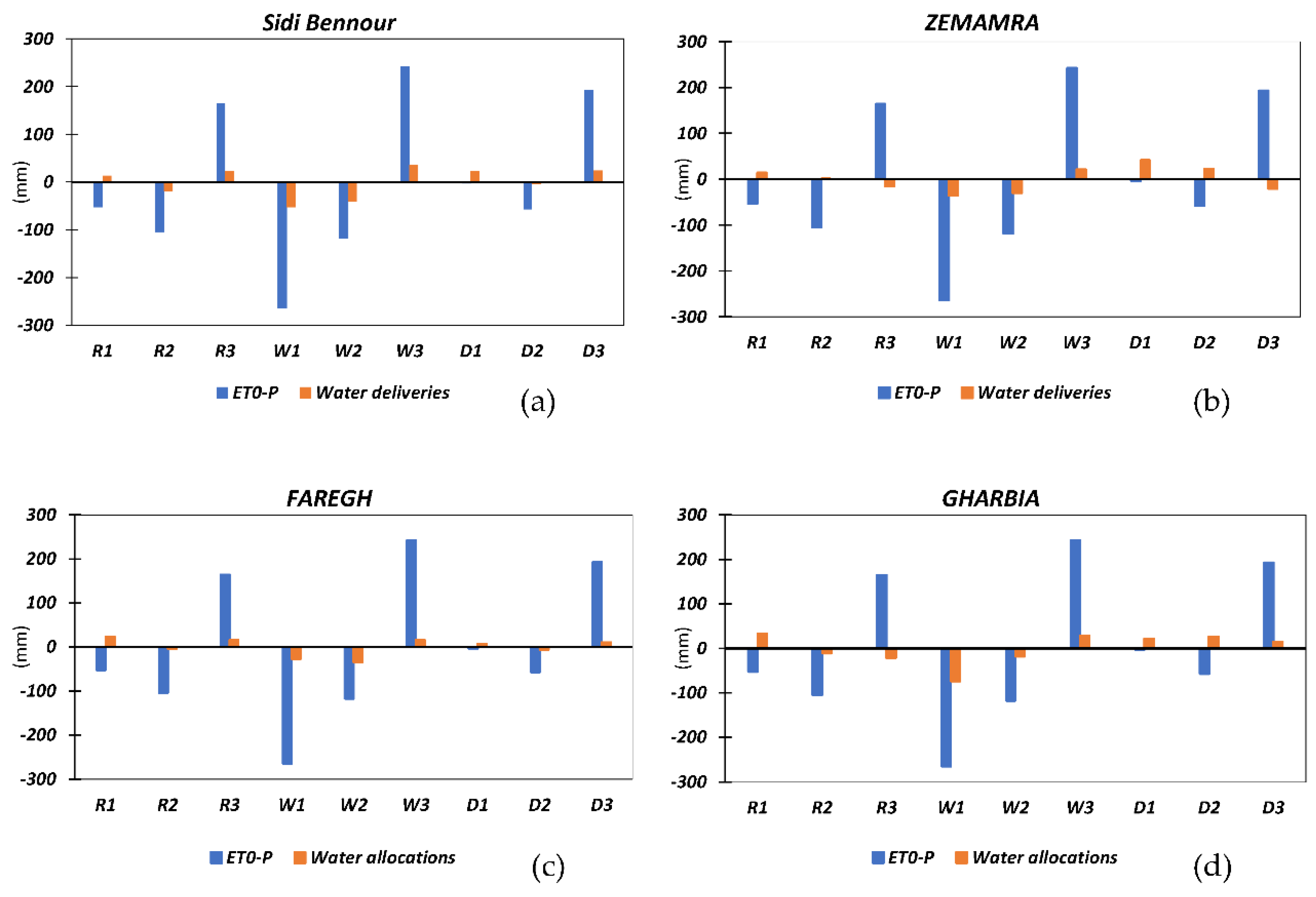
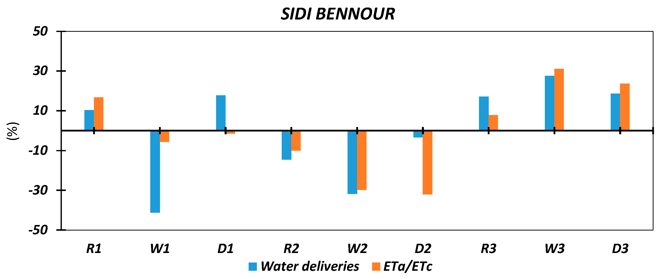
• Sidi Bennour: Overall, the relative anomalies in ET_a/ET_c and W_d (Figure 10) are consistent, i.e., they have the same sign and comparable magnitude. In the third quarter (April-June) higher than average W_d apparently lead to higher than average ET_a/ET_c. To the contrary, in the second quarter (January–March) lower than average W_d seem to induce lower than average (ET_a/ET_c) In the first quarter (October–December) the response of W_d to ET₀-P and of ET_a/ET_c to W_d is more variable across the reference, wet and dry year, possibly due to high precipitation in this period of the year.
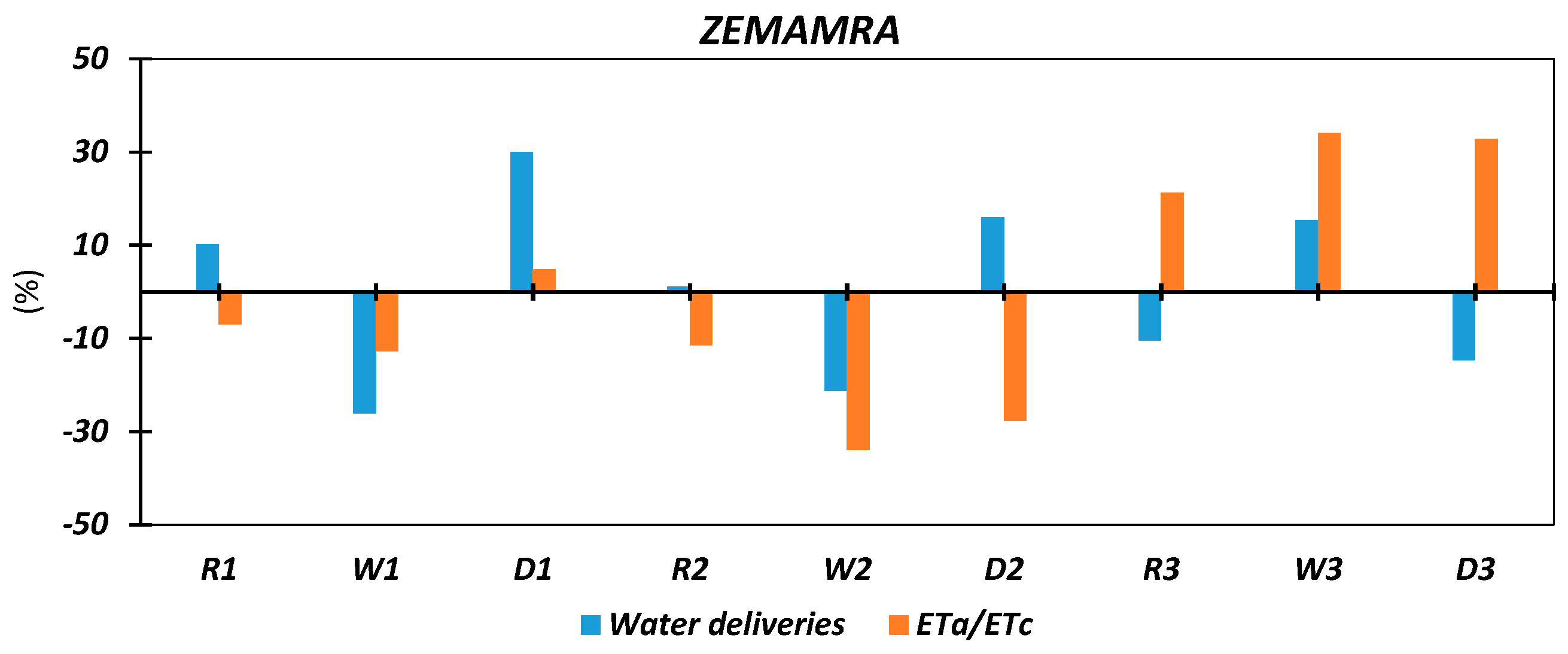
• Zemamra: The pattern in relative anomalies is more complex than in the case of Sidi Bennour. W_d in the first and second quarter (Figure 11) is lower than average in the wet year while it is higher than average in the third quarter. On the other hand, W_d is higher than average in the first and second quarter while it is lower in the third quarter of both dry and reference year. The response of ET_a/ET_c to changes in W_d is more variable than in the case of Sidi Bennour.
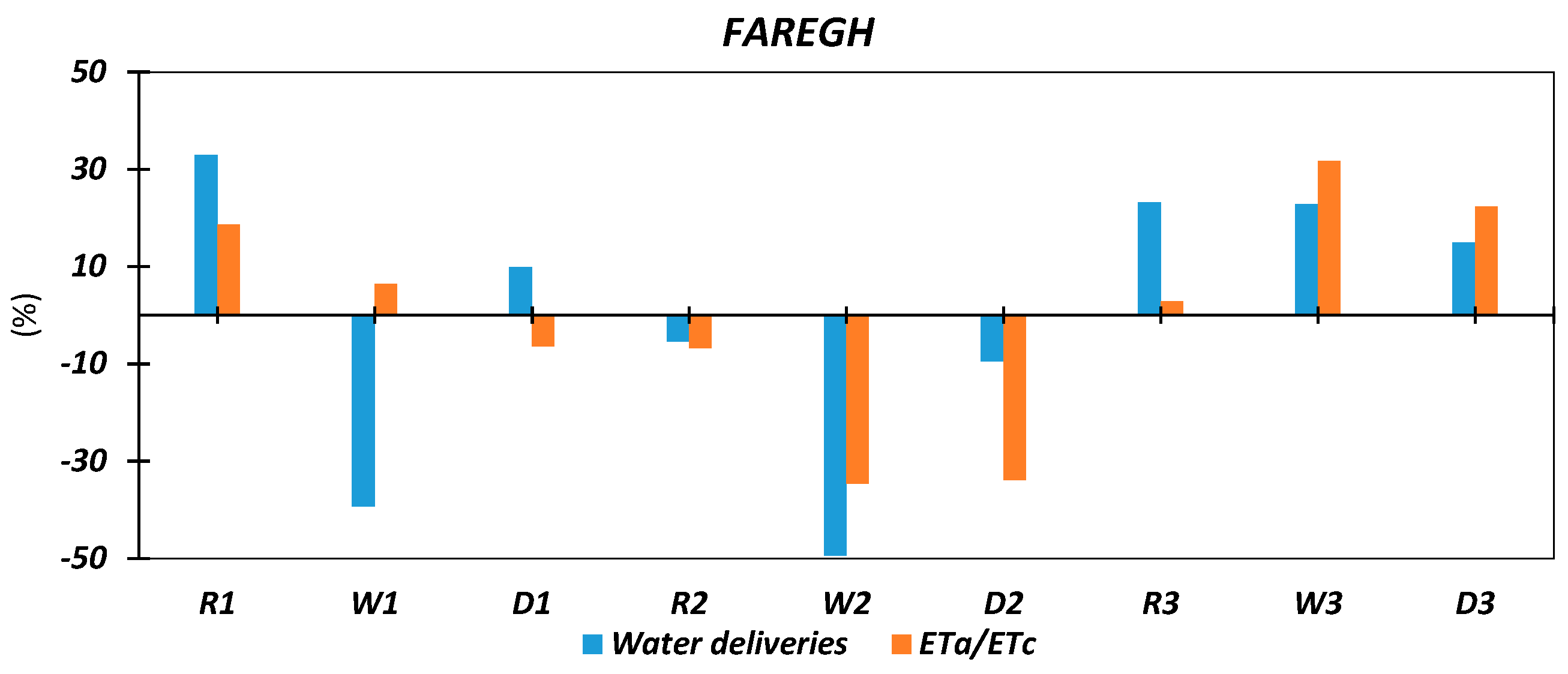
• Fregh: In most cases, relative anomalies in ET_a/ET_c have the same sign and similar magnitude as anomalies in W_d (see Figure 12). As in the case of Sidi Bennour W_d was higher than average in the third (generally drier) quarter of all the three years. To the contrary, W_d was lower than average in the second quarter, also in all the years. Anomalies in W_d were more variable in the first quarter. Higher than average ET_a/ET_c was generally associated with higher than average W_d, with the notable exception of the first quarter of the wet year. Lower than average ET_a/ET_c was clearly associated with lower than average W_d in the second quarter of all years.
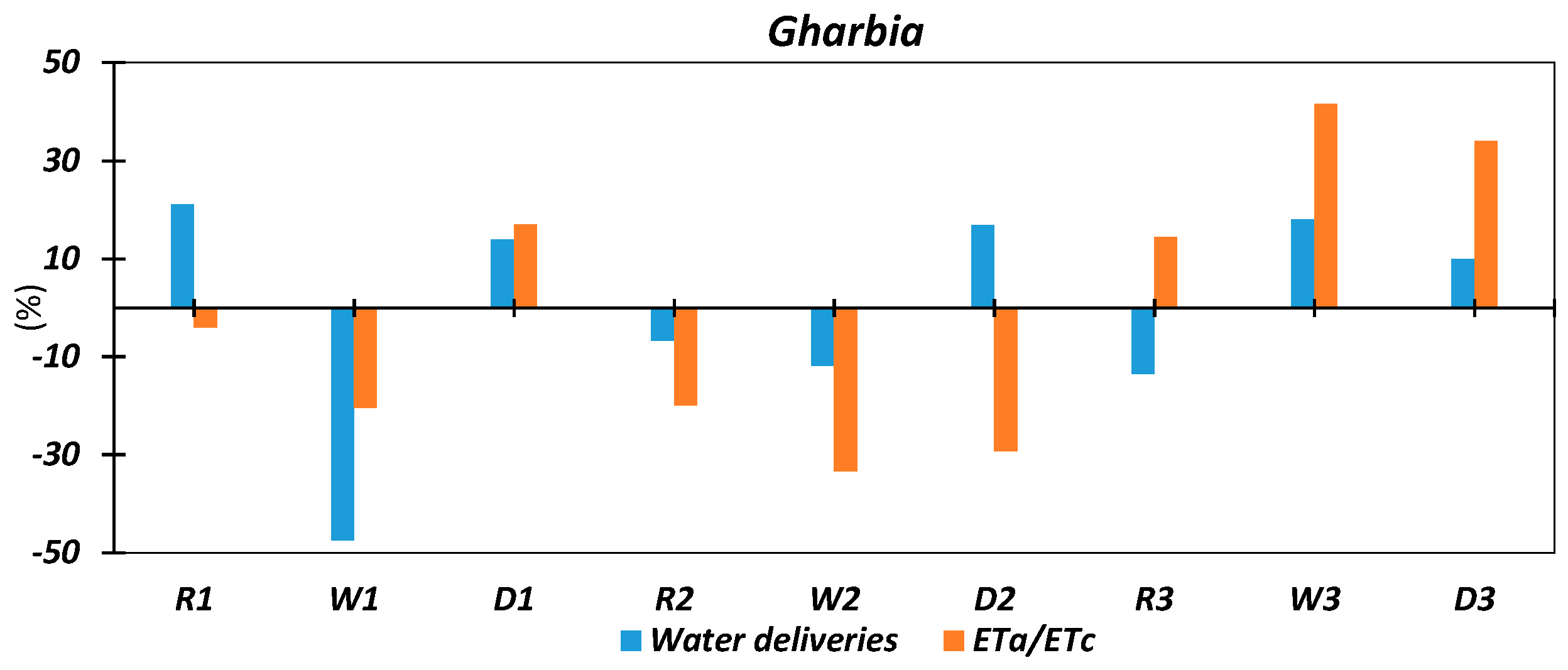
• Gharbia: Additionally, in this district relative anomalies in ET_a/ET_c and W_d were consistent in most cases (Figure 13). Large negative anomalies in ET_a/ET_c in the first and the second quarter of the wet year and in the second quarter of the reference year were associated with lower than average W_d, with the negative anomaly being rather large in the first quarter in the wet year. Similar responses were observed in the other districts particularly in Zemamra. Relative anomalies in ET_a/ET_c were much larger than relative anomalies in W_d in the second and third quarter of the wet year, although of opposite sign in both quarters.

Overall it should be noted that W_d is higher than average in the 3rd quarter in all districts and for all years, likewise ET_a/ET_c, thus suggesting a beneficial adaptation in irrigation management to the higher water requirements in late spring/early summer. As noted earlier (see also Figure 6), it appears that a relatively small increment in W_d, although much smaller than the increment in ET₀-P, is sufficient to achieve a lower evapotranspiration deficit, i.e., an increment in ET_a/ET_c.

5. Discussion

5.1. Inter- and Intra-Annual Climatic Variability

The analysis presented in Section 4.1 documented the large inter and intra-annual variability of ET₀-P, but did not provide evidence on a real adaptive response of the water management system. Water delivery did change in wet and dry years but mainly as consequence of the reservoir operational rules in response to changes in water inflow and stock. In 1995–1996 an exceptionally large inflow led to completely fill up the reservoir with a delay of approximately one year and to slowly increasing water deliveries over a period of a few years. The subsequent dry spell led to sharply reduced water deliveries and residual water storage. These statements are supported by the observed poor correlation of W_d with ET₀-P, although an analysis of actual rather than atmospheric water demand would be needed for a robust assessment. In the period 1992–2016 there was just one dry spell, although rather long from 2000 to 2009. From the point of view of adaptive water management, it would be rather relevant to analyze a much longer climate record to estimate the frequency of such events, in order to develop an adaptation strategy either by increasing water storage capacity or by controlling land use to balance water supply and actual water demand. These findings are in line with the review on the evolution of the irrigation management system in Morocco presented by [54], which emphasized the urgent need for renewed efforts by the ORMVA-s towards better implementation and performance of participatory irrigation management. Particularly, this author emphasized that irrigation water conservation implies the adoption of measures to modify water demands and maximize efficiency in water use.

Likewise, the detailed analysis of actual water demand and water use versus water supply in extreme wet and dry years did not provide evidence of seasonal adaptation of water delivery. Again, the operational rules of ORMVAD promote short term adaptation, e.g., on a weekly basis, to water availability (precipitation), rather than to the seasonal evolution of land use and crop water use. To further support this statement, we note that no systematic relation was observed between ET_a/ET_c and W_d under the extreme wet (2014–2015) and the extreme dry (2015–2016) conditions with very different ET₀-P.

Our analysis of the response of ET_a/ET_c to W_d for all the CGRs did provide evidence of a larger variability in such response in the CGRs where drip irrigation is dominant. This suggests larger differences in the efficiency of water application notwithstanding the higher water application efficiency of drip irrigation [55].

It should be taken into account that we have analyzed the response of W_d to ET₀-P using seasonal data and the response of ET_a/ET_c to W_d using quarterly data, this approach may have hidden the subtle aspects of the response of crop water use to short term adaptation in water delivery in relation with precipitation events.

5.2. Response to Climatic Variability

Sidi Bennour (Figure 10): Relative changes in water delivery and relative evapotranspiration ET_a/ET_c were comparable for the first, second, and third quarters in the reference year, in the second and third quarters in the wet year and in the third quarter in the dry year. In the first quarter of the wet year the relative anomalies in ET_a/ET_c were much smaller than relative anomalies in water delivery. In this case water delivery was reduced taking into account the very large precipitation (P) in same quarter. Specifically, the precipitation in this quarter (

Table 4. Doukkala irrigation scheme: Quarterly precipitation (P) of wet, dry and reference years.

Growing Season	2013–2014	2014–2015	2015–2016
Quarter	Precipitation (mm)
October–December	30.5	251.4	54.6
January–March	89.1	99.3	89.4
April–June	64.3	2	77.8

) was 226% of the average over all quarters and all years. The large precipitation was sufficient to maintain high ET_a/ET_c. In the 2nd quarter of the dry year, the water delivery was not increased to compensate the larger than average ET₀-P and was even slightly lower than the average. As a consequence, ET_a/ET_c was equal to 0.66, i.e., much lower than the average over all quarters and all years. In the first quarter of the dry year, ET₀-P was much larger than in the same quarter of the other years. Water deliveries were increased by 18% above the average, which apparently was sufficient to maintain the ET_a/ET_c roughly constant. This is what adaptive irrigation water management should achieve.

Zemamra (Figure 11): In the 3rd quarter of the wet year ET_a/ET_c was much larger than the average. This is explained by the water deliveries which were 30% above the average in the same quarter. In addition, the precipitation in the first quarter of the same year was 226% higher than the average, thus fully replenishing the soil water reservoir to maintain high ET_a/ET_c. In the 1st quarter of the dry year water deliveries were increased by 30% over the average, which was sufficient to maintain ET_a/ET_c roughly constant. In the 2nd quarter of the dry year, water deliveries were 16% higher than the average while ET_a/ET_c was 27% lower than the average. This can be explained by the precipitation in the first quarter being 29% lower than average. A similar response in ET_a/ET_c was observed in the 1st quarter of the reference year when deliveries were 10% higher than average, but the precipitation was 65% lower than the average.

Faregh (Figure 12): The relative changes in deliveries and ET_a/ET_c were roughly similar in the 1st, 2nd and 3rd quarter of the reference year, in the 2nd and 3rd quarter of the wet year and the 3rd quarter of the dry year. The 1st quarter of the wet year and the 3rd quarter of the reference year, water deliveries were adapted successfully to maintain ET_a/ET_c roughly constant notwithstanding the large variations in ET₀-P, which was 134% lower than average in the 1st case and 83% higher than average in the second case. In the 2nd quarter of the dry year water deliveries were correctly reduced in response to ET₀-P being 30% lower than average with precipitation being 16% higher than average but concentrated in few days in February. This led to a 32% decrease in ET_a/ET_c.

Gharbia (Figure 13): The relative changes in ET_a/ET_c and water deliveries had a similar magnitude in the 1st, 2nd and the third quarter of the wet year, in the 1st and 3rd quarter of the dry year and in the 2nd quarter of the reference. In the 2nd quarter of the dry year water deliveries were 16% higher than average, notwithstanding ET₀-P being 30% lower than average with precipitation being 16% higher than average but concentrated in few days in February. This led to a 29% decrease in ET_a/ET_c.

6. Conclusions

This study evaluated whether the rigid water deliveries rules applied by ORMVAD, the water management authority of the Doukkala irrigation scheme, combined with the autonomous decision by farmers at each rotational interval, would lead to actual delivery of irrigation water consistent with an assessment of demand based on established agro-hydrological practices. Water delivery did respond to inter-annual variability in hydrological conditions, but rather to water inflows to reservoirs than to atmospheric water demand ET₀-P. This notwithstanding, we have shown several instances where anomalies in water delivery do correlate with anomalies in ET₀-P, which is surprising to some extent, since no such quantitative evaluation of water requirements plays a role in the decision by farmers about requesting water delivery.

Our evaluation of the crop response to variable water delivery showed that in 70%–90% of the cases the ratio ET_a/ET_c changes with water delivery as expected, i.e., it increases with larger water deliveries and vice versa. There are a few cases, however, where anomalies in ET_a/ET_c and W_d have the opposite sign. Most likely this is due to the distribution in the time of precipitation and water delivery, but we do not have sufficiently detailed data to evaluate this hypothesis.

If we assume that the decision by farmers about whether or not to request water at a given time is based on a perception of ET₀-P, this conclusion raises a new research question, i.e., whether farmers perceive correctly an impending water shortage and take the right decision about requesting delivery of irrigation water in a given rotational interval.

References

- Schilling, J.P.; Freier, K.; Hertig, E.; Scheffran, J. Climate change, vulnerability and adaptation in North Africa with focus on Morocco. Agric. Ecosyst. Environ. 2012, 156, 12–26. [Google Scholar] [CrossRef]
- FAO. AQUASTAT Main Database; Food and Agriculture Organization of the United Nations (FAO): Rome, Italy, 2016; Available online: http://www.fao.org/nr/water/aquastat/data/query/index.html?lang=fr (accessed on 29 September 2019).
- Stakhiva, E.; Stewart, B. Needs for climate information in support of decision-making in the water sector. Procedia Environ. Sci. 2010, 1, 102–119. [Google Scholar] [CrossRef]
- National Research Council of the National Academies. Adaptive Management for Water Resources Project Planning; The National Academies Press: Washington, DC, USA, 2004. [Google Scholar] [CrossRef]
- Sharma, K.D.; Gosain, A.K. Application of Climate Information and Predictions in Water Sector: Capabilities. Procedia Environ. Sci. 2010, 1, 120–129. [Google Scholar] [CrossRef] [Green Version]
- Tanaka, S.K.; Zhu, T.; Lund, J.R.; Howitt, R.E.; Jenkins, M.W.; Pulido, M.A.; Tauber, M.; Ritzema, R.S.; Ferreira, I.C. Climate warming and water management adaptation for California. Clim. Chang. 2006, 76, 361–387. [Google Scholar] [CrossRef]
- Drieschova, A.; Giordano, M.; Fischhendler, I. Governance mechanisms to address flow variability in water treaties. Glob. Environ. Chang. 2008, 18, 285–295. [Google Scholar] [CrossRef]
- Yang, Y.; Shang, S.; Jiang, L. Remote sensing temporal and spatial patterns of evapotranspiration and the responses to water management in a large irrigation district of North China. Agric. For. Meteorol. 2012, 164, 112–122. [Google Scholar] [CrossRef]
- Organisation for Economic Co-Operation and Development (OECD). Water Ressources Allocation: Sharing Risks and Opportunities, Case of Spain; OECD: Paris, France, 2015. [Google Scholar] [CrossRef]
- Akdim, N.; Alfieri, S.M.; Habib, A.; Choukri, A.; Cheruiyot, E.; Labbassi, K.; Menenti, M. Monitoring of Irrigation Schemes by Remote Sensing: Phenology versus Retrieval of Biophysical Variables. Remote Sens. 2014, 6, 5815–5851. [Google Scholar] [CrossRef] [Green Version]
- Zargar, A.; Sadiq, R.; Naser, B.; Khan, F.I.; Naser, G. A review of drought indices. Environ. Rev. 2011, 19, 333–349. [Google Scholar] [CrossRef]
- Tsakiris, G.; Vangelis, H. Establishing a drought index incorporating evapotranspiration. Eur. Water 2005, 9, 3–11. [Google Scholar]
- Palmer, W.C. Meteorological Drought; Research Paper N° 451965; Office of Climatology, U.S. Weather Burau: Washington, DC, USA, 1965.
- Vicente-Serrano, M.S.; Beguería, S.; López-Moreno, J.I. A multiscalar drought index sensitive to global warming: The standardized precipitation evapotranspiration index. J. Clim. 2010, 23, 1696–1718. [Google Scholar] [CrossRef]
- Lei, H.; Yang, D. Interannual and seasonal variability in evapotranspiration and energy partitioning over an irrigated cropland in the North China Plain. Agric. For. Meteorol. 2010, 150, 581–589. [Google Scholar] [CrossRef]
- Zeng, L.; Song, K.; Zhang, B.; Wang, Z. Spatial mapping of actual evapotranspiration and water deficit with MODIS products in the Songnen Plain, northeast China. In Proceedings of the 2010 IEEE International Geoscience and Remote Sensing Symposium, Honolulu, HI, USA, 25–30 July 2010; pp. 879–882. [Google Scholar] [CrossRef]
- Li, X.; Cheng, G.; Liu, S.; Xiao, Q.; Ma, M.; Jin, R.; Che, T.; Liu, Q.; Wang, W.; Qi, Y.; et al. Heihe watershed allied telemetry experimental research (HiWater) scientific objectives and experimental design. Bull. Am. Meteorol. Soc. 2013, 94, 1145–1160. [Google Scholar] [CrossRef]
- Gowda, P.H.; Chavez, J.L.; Colaizzi, P.D.; Evett, S.R.; Howell, T.A.; Tolk, J.A. ET mapping for agricultural water management: Present status and challenges. Irrig. Sci. 2008, 26, 223–237. [Google Scholar] [CrossRef]
- Li, Z.-L.; Tang, R.; Wan, Z.; Bi, Y.; Zhou, C.; Tang, B.; Yan, G.; Zhang, X. A review of current methodologies for regional Evapotranspiration estimation from remotely sensed data. Sensors 2009, 9, 3801–3853. [Google Scholar] [CrossRef] [PubMed]
- Hu, G.; Jia, L.; Massimo, M. Comparison of MOD16 and LSA-SAF MSG evapotranspiration products over Europe for 2011. Remote Sens. Environ. 2014, 156, 510–526. [Google Scholar] [CrossRef]
- Menenti, M.; Choudhury, B.J. Parameterization of land surface evaporation by means of location dependent potential evaporation and surface temperature range. In Exchange Processes at the Land Surface for a Range of Space and Time Scales, Proceedings of the Yokohama Symposium, Yokohama, Japan, 21–23 July 1993; IAHS Publ. No. 212; IAHS Press: Wallingford, UK, 1993; pp. 561–568. [Google Scholar]
- Norman, J.M.; Kustas, W.P.; Humes, K.S. Source approach for estimating soil and vegetation energy fluxes in observations of directional radiometric surface temperature. Agric. For. Meteorol. 1995, 77, 263–293. [Google Scholar] [CrossRef]
- Bastiaanssen, W.; Pelgrum, H.; Wang, J.; Ma, Y.; Moreno, J.; Roerink, G.; van der Wal, T. A remote sensing surface energy balance algorithm for land (SEBAL) 1. Formulation. J. Hydrol. 1998, 212, 213–229. [Google Scholar] [CrossRef]
- Bastiaanssen, W.; Pelgrum, H.; Wang, J.; Ma, Y.; Moreno, J.; Roerink, G.; van der Wal, T. A remote sensing surface energy balance algorithm for land (SEBAL): 2. Validation. J. Hydrol. 1998, 212, 213–229. [Google Scholar] [CrossRef]
- Roerink, G.J.; Su, Z.; Menenti, M. S-SEBI: A simple remote sensing algorithm to estimate the surface energy balance. Phys. Chem. Earth Part B Hydrol. Oceans Atmos. 2000, 25, 147–157. [Google Scholar] [CrossRef]
- Su, Z. The Surface Energy Balance System (SEBS) for estimation of turbulent heat fluxes. Hydrol. Earth Syst. Sci. 2002, 6, 85–100. [Google Scholar] [CrossRef]
- Ghilain, N.; Arboleda, A.; Gellens-Meulenberghs, F. Evapotranspiration modelling at large scale using near-real time MSG SEVIRI derived data. Hydrol. Earth Syst. Sci. 2011, 15, 771–786. [Google Scholar] [CrossRef] [Green Version]
- Sánchez, J.; Kustas, W.; Caselles, V.; Anderson, M.; Anderson, M. Modelling surface energy fluxes over maize using a two-source patch model and radiometric soil and canopy temperature observations. Remote Sens. Environ. 2008, 112, 1130–1143. [Google Scholar] [CrossRef]
- Miralles, D.G.; De Jeu RA, M.; Gash JH, C.; Holmes TR, H.; Dolman, A.J. Magnitude and variability of land evaporation and its components at the global scale. Hydrol. Earth Syst. Sci. 2011, 15, 967–981. [Google Scholar] [CrossRef] [Green Version]
- Mu, Q.; Zhao, M.; Running, S.W. Improvements to a MODIS global terrestrial evapotranspiration algorithm. Remote Sens. Environ. 2011, 115, 1781–1800. [Google Scholar] [CrossRef]
- Ruhoff, A.L.; Paz, A.R.; Aragão, L.E.O.C.; Mu, Q.; Malhi, Y.; Collischonn, W.; Rocha, H.R.; Running, S.W.; Ruhoff, A. Assessment of the MODIS global evapotranspiration algorithm using eddy covariance measurements and hydrological modelling in the Rio Grande basin. Hydrol. Sci. J. 2013, 58, 1658–1676. [Google Scholar] [CrossRef]
- Hemakumara, H.M.; Chandrapala, L.; Moene, A.F. Evapotranspiration fluxes over mixed vegetation areas measured from large aperture scintillometer. Agric. Water Manag. 2003, 58, 109–122. [Google Scholar] [CrossRef]
- Hofste, R.W. Comparative Analysis among Near-Operational Evapotranspiration Products for the Nile Basin Based on Earth Observations First Steps towards an Ensemble Product. Master’s Thesis, Delft University of Technology, Delft, The Netherlands, 2014. [Google Scholar]
- Ferré, M.; Ruhard, J.P. Les bassins des Abda-Doukkala et du Sahel de Azemmour à Safi. Notes Mém. Serv. Géol. 1975, 23, 261–297. [Google Scholar]
- Guemimi, A. Plan D’action D’économie de L’eau Dans le Périmètre Des Doukkala. In Proceedings of the La Modernisation de L’agriculture Irriguée, Actes du Séminaire Euro-Méditerranéen, Thème 1: Aspects Techniques de la Modernisation des Systèmes Irriguès, Rabat, Maroc, 19–23 April 2004; pp. 1–10. [Google Scholar]
- Brouwer, C.; Prins, K.; Heibloem, M. Irrigation Water Management: Irrigation Scheduling. In Training Manual No. 4; 1989; Volume 4, p. 66. Available online: ftp://ftp.fao.org/agl/aglw/fwm/Manual4.pdf (accessed on 29 September 2019).
- Akdim, N. Les Données D’observation de la Terre Pour L’evaluation de la Performance de L’irrigation dans un Contexte de Climat Semi-Aride: Perimetre Irrigué des Doukkala_Maroc. Ph.D. Thesis, Universite Chouaib Doukkali, El Jadida, Maroc, 2014. [Google Scholar]
- Zanter, K. Landsat-8 (L8) Data Users Handbook; Department of the Interior, U.S. Geological Survey: Reston, VA, USA, 2016; Volume 8, p. 1993.
- Chavez, J.G. Image-based atmospheric corrections-revisited and improved. Photogramm. Eng. Remote 1996, 62, 1025–1036. [Google Scholar]
- Monteith, J.L. Evaporation and Environment. Symp. Soc. Exp. Biol. 1965, 19, 205–234. [Google Scholar]
- Allen, R.G.; Pereira, L.S.; Raes, D.; Smith, M. FAO Irrigation and Drainage Paper No. 56. Crop Evapotranspiration (guidelines for computing crop water requirements). Irrig. Drain. 1998, 300, D05109. [Google Scholar] [CrossRef]
- Congedo, L. Semi-Automatic Classification Plugin Documentation Release 4.8.0.1; Project: Semi-Automatic Classification Plugin; Sapienza University of Rome: Roma, Italy, 2016; Volume 4. [Google Scholar] [CrossRef]
- Jiménez-Muñoz, J.C.; Sobrino, J.A.; Skoković, D.; Mattar, C.; Cristóbal, J. Land surface temperature retrieval methods from landsat-8 thermal infrared sensor data. IEEE Geosci. Remote Sens. Lett. 2014, 11, 1840–1843. [Google Scholar] [CrossRef]
- Latif, M.S. Land Surface Temperature Retrival of Landsat-8 Data Using Split Window Algorithm—A Case Study of Ranchi District. Int. J. Eng. Dev. Res. 2014, 2, 3840–3849. [Google Scholar]
- Azzali, S.; Menenti, M.; Meuwissen, I.J.M.; Visser, T.M.N. Application of remote sensing techniques to map crop coefficients in an Argentinian irrigation scheme. In Advances in Water Resources Technology; Tsakiris, G., Ed.; Balkema: Rotterdam, The Netherlands, 1991; pp. 637–643. [Google Scholar]
- Belmonte, A.C.; Jochum, A.M.; GarcÍa, A.C.; Rodríguez, A.M.; Fuster, P.L. Irrigation management from space: Towards user-friendly products. Irrig. Drain. Syst. 2005, 19, 337–353. [Google Scholar] [CrossRef]
- D’Urso, G.; Menenti, M. Mapping crop coefficients in irrigated areas from Landsat TM images. In European Symposium on Satellite Remote Sensing II, Remote Sensing for Agriculture, Forestry, and Natural Resources; SPIE: Bellingham, WA, USA, 1995; Volume 2585, pp. 41–47. [Google Scholar] [CrossRef]
- D’Urso, G. Simulation and Management of On-Demand Irrigation Systems: A Combined Agrohydrological and Remote Sensing Approach. Ph.D. Thesis, Wageningen University, Wageningen, The Netherlands, 2001. [Google Scholar]
- D’Urso, G. Current Status and Perspectives for the Estimation of Crop Water Requirements from Earth Observation. Ital. J. Agron. 2010, 107–120. [Google Scholar] [CrossRef]
- Bastiaanssen, W. Regionalization of Surface Flux Densities and Moisture Indicators in Composite Terrain: A Remote Sensing Approach under Clear Skies in Mediterranean Climates. Ph.D. Thesis, Wageningen Agricultural University, Wageningen, The Netherlands, 1995. [Google Scholar]
- Allen, R.G.; Tasumi, M.; Trezza, R.; Waters, R.; Bastiaanssen, W. Sebal Surface Energy Balance Algorithms for Land Idaho Implementation Advanced Training and User’s Manual; Waters Consulting: Nelson, BC, Canada; University of Idaho: Moscow, ID, USA; WaterWatch, Inc.: Wageningen, The Netherlands, 2002; pp. 1–98. [Google Scholar]
- Bastiaanssen, W.G.M. SEBAL-based sensible and latent heat fluxes in the irrigated Gediz Basin, Turkey. J. Hydrol. 2000, 229, 87–100. [Google Scholar] [CrossRef]
- Allen, R.G.; Tasumi, M.; Trezza, R. Satellite-Based Energy Balance for Mapping Evapotranspiration with Internalized Calibration (METRIC)—Model. J. Irrig. Drain. Eng. 2007, 133, 380–394. [Google Scholar] [CrossRef]
- Choukr-Allah, R. Participatory irrigation management in MOROCCO. Water Energy Int. 2004, 57, 17–23. [Google Scholar]
- Irmak, S.; Odhiambo, L.O.; Kranz, W.L.; Eisenhauer, D.E. Irrigation Efficiency and Uniformity, and Crop Water Use Efficiency. Biol. Syst. Eng. 2011, 59, 873–884. [Google Scholar] [CrossRef]