Article

Multi-Objective Operation of Cascade Hydropower Reservoirs Using TOPSIS and Gravitational Search Algorithm with Opposition Learning and Mutation

1
School of Hydropower and Information Engineering, Huazhong University of Science and Technology, Wuhan 430074, China
2
Bureau of Hydrology, ChangJiang Water Resources Commission, Wuhan 430010, China
3
Tsinghua Sichuan Energy Internet Research Institute, Chengdu 610200, China
4
State Grid Sichuan Electric Power Research Institute, Chengdu 610072, China
*
Author to whom correspondence should be addressed.
Water 2019, 11(10), 2040; https://doi.org/10.3390/w11102040
Submission received: 27 August 2019 / Revised: 27 September 2019 / Accepted: 28 September 2019 / Published: 29 September 2019
(This article belongs to the Special Issue Advances in Hydrologic Forecasts and Water Resources Management )

Abstract

:
In this research, a novel enhanced gravitational search algorithm (EGSA) is proposed to resolve the multi-objective optimization model, considering the power generation of a hydropower enterprise and the peak operation requirement of a power system. In the proposed method, the standard gravity search algorithm (GSA) was chosen as the fundamental execution framework; the opposition learning strategy was adopted to increase the convergence speed of the swarm; the mutation search strategy was chosen to enhance the individual diversity; the elastic-ball modification strategy was used to promote the solution feasibility. Additionally, a practical constraint handling technique was introduced to improve the quality of the obtained agents, while the technique for order preference by similarity to an ideal solution method (TOPSIS) was used for the multi-objective decision. The numerical tests of twelve benchmark functions showed that the EGSA method could produce better results than several existing evolutionary algorithms. Then, the hydropower system located on the Wu River of China was chosen to test the engineering practicality of the proposed method. The results showed that the EGSA method could obtain satisfying scheduling schemes in different cases. Hence, an effective optimization method was provided for the multi-objective operation of hydropower system.

1. Introduction

With the merits of low pollution emission and high work efficiency, hydropower is seen as one of the most important renewable energy sources and usually shoulders many different kinds of management requirements, in practice [1,2,3]. For hydropower enterprises, it is preferred to make full use of the water resources to obtain the maximum economic benefit [4]; for power systems, the flexible hydropower generators are often asked to respond to the peak loads and smooth the energy demand curves [5]. Under such a background, the operation optimization of cascade hydropower reservoirs balancing a power generation and peak operation has become one of the most important tasks in both water resource systems and modern power systems [6]. However, as far as we know, there are few reports that have addressed this engineering problem, and therefore, the goal of this research was to refill this huge gap between theoretical research and engineering requirement.
From a mathematical point of view, the target problem was a typical multi-objective constrained optimization problem with a set of complex equality or inequality constraints [7], and many classical methods have been successfully developed by scholars, during the past decades [8,9,10,11,12,13], like linear programming [14], quadratic programming [15], dynamic programming [16,17,18], Lagrange relaxation, and network optimization [19,20,21]. However, the hydropower operation problem is usually modeled with nonlinear characteristic curves, physical constraints, or objective functions [22,23,24]. The above-mentioned traditional methods might fail to address the complexity due to various defects, like dimensionality problem [25], high computational burden [26], duality gap [27], or parameter tuning [28,29,30]. In recent years, with the booming development of computer technology, many evolutionary algorithms have been proposed to resolve these kind of problems [31,32,33], like genetic algorithm (GA) [34], differential evolution (DE) [35,36], particle swarm algorithm (PSO) [37,38,39,40], cuckoo search (CS) [41], Covariance Matrix Adaptation Evolution Strategy with a Directed Target to Best Perturbation (CMA-ES-DTBP) [42], and a clustered adaptive teaching–learning-based optimization (CATLBO) [43]. Compared with traditional methods, the evolutionary algorithms can produce satisfying solutions in most cases, regardless of the problem features (like continuity or nonconvexity) [44,45,46]. However, due to the premature convergence, evolutionary algorithms often fall into local optima, which have limited their widespread applications in practical engineering [47,48,49,50]. Hence, it is necessary to find some effective modified strategies to enhance the performances of the evolutionary algorithms in the hydropower operation problems.
Gravitational search algorithm (GSA) is a famous evolutionary algorithm based on the laws of gravity and mass interactions in Newtonian mechanics [51,52,53]. Although GSA outperforms the standard PSO and GA methods in many problems, certain defects (like exploration–exploitation imbalance and local convergence) still exist. For improving the performance of the standard GSA method, this study proposes an enhanced GSA algorithm (EGSA) where three modified strategies (opposition learning strategy, mutation search strategy, and elastic-ball modification strategy) are integrated to alleviate the premature convergence problem. Several famous test functions are used to verify the feasibility of the developed method in solving the global optimization problems, and the results demonstrate that the modified strategies could effectively enhance the convergence speed and the global search ability of the population at the same time. Then, two specific strategies were embedded into the EGSA method to help address the multi-objective operation problem of a hydropower system—(i) the practical constraint handling strategy for solution feasibility and (ii) the Technique for Order Preference by Similarity to an Ideal Solution (TOPSIS) for multi-objective decision. Finally, the EGSA method was applied to address the operation optimization of cascade hydropower system in the Wu River of China. The simulations showed that the proposed method could produce better scheduling schemes in different application scenarios.
The rest of this paper is organized as below—the EGSA method is presented in Section 2; several benchmark functions are used to verify the performance of the EGSA method in Section 3; Section 4 gives the mathematical model for the multi-objective operation of cascade hydropower reservoirs; Section 5 compares the results of different methods; and the conclusions are drawn in the end.

2. Enhanced Gravitational Search Algorithm (EGSA)

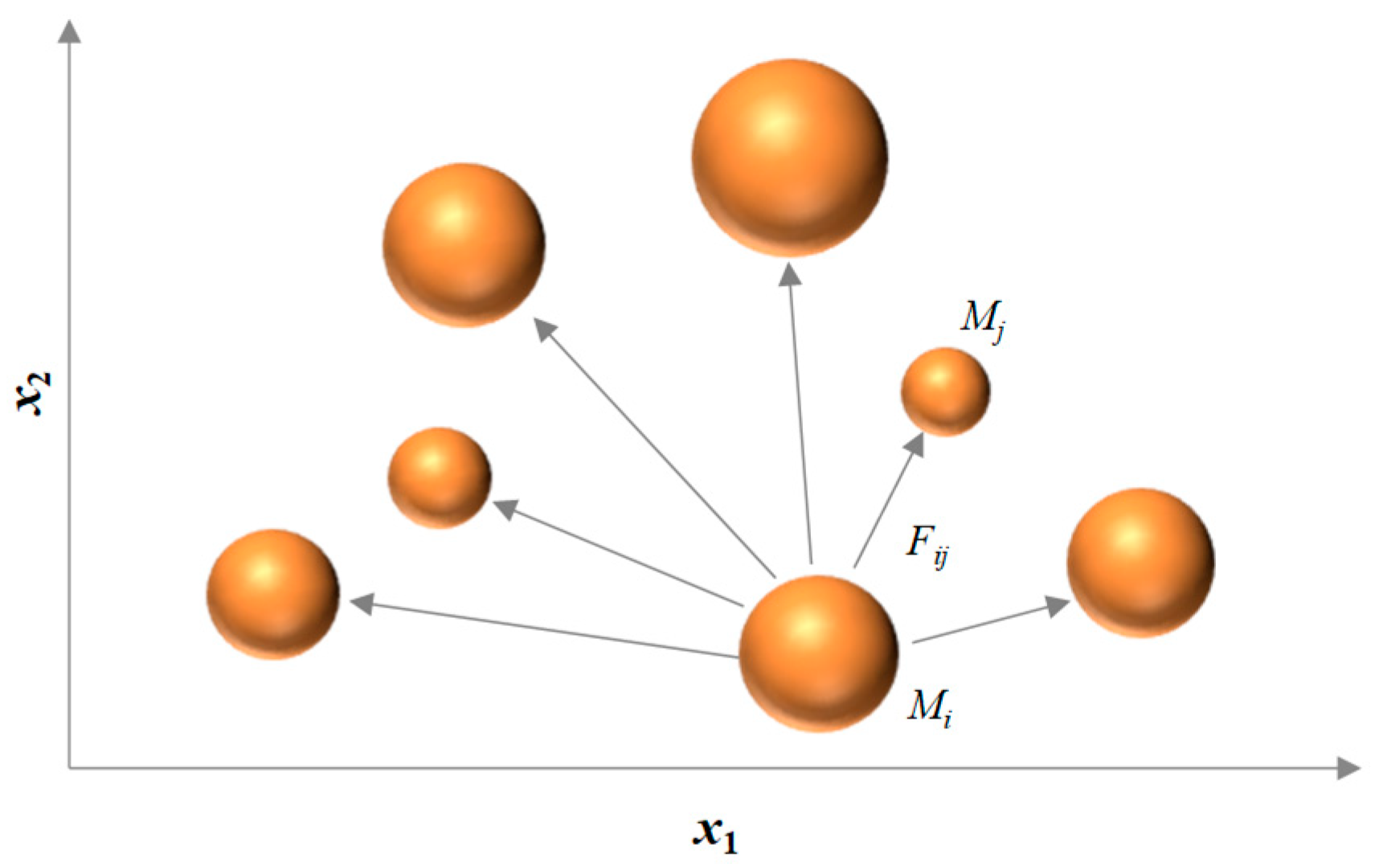
2.1. Gravitational Search Algorithm (GSA)

GSA is a novel swarm-based evolutionary algorithm inspired by the universal gravitation and mass interactions in classical Newton’s Mechanics [54]. In GSA, the potential solution for the target optimization problems is considered to be an agent with a certain quality, and all the agents are attracted by other agents via the so-called gravity force, which can effectively help the swarm share the acquired beneficial information about the surrounding [55]. Figure 1 draws the sketch map of the GSA method. It can be seen that during the evolutionary process, the gravity force of the two agents is directly and inversely proportional to their qualities and distances, respectively; while the agents with better performances usually have larger attraction forces and slower velocity than those agents with smaller quality. By these means, all agents gradually finish the transition from the global exploration to local exploitation in the decision space, which help the swarm obtain the global optima.
Without a loss of generality, it is assumed that there are N agents in the evolutionary swarm to determine the optimal solution for the minimization–optimization problem with D variables, and then the position of the ith agent at the kth iteration ( X i ( k ) for short) can be expressed as follows:
X i ( k ) = ( x i 1 ( k ) , , x i d ( k ) , , x i D ( k ) )
where x i d ( k ) is the position of the ith agent in the dth dimension at the kth iteration.
In the evolutionary process, the gravitational force of the nth agent acting on the ith agent in the dth dimension at the kth iteration can be expressed as follows:
F i n d ( k ) = G ( k ) M i ( k ) × M n ( k ) R i n ( k ) + φ ( x i d ( k ) x n d ( k ) )
where M i ( k ) and M n ( k ) are the gravitational masses of the ith agent and the nth agent at the kth iteration, respectively. R i n ( k ) = | | X i ( k ) , X n ( k ) | | 2 is the Euclidian distance between the ith agent and the nth agent at the kth iteration. φ is a small constant used to prevent the denominator being 0. G ( k ) is the gravitational constant of the swarm at the kth iteration, which is dynamically updated by:
G ( k ) = G 0 × exp ( α k k ¯ )
where G 0 is the initial gravitational constant. α is the attenuation coefficient. k ¯ is the maximum number of iterations.
After obtaining the latest positions of all agents, the mass of the ith agent at the kth iteration ( m i ( k ) for short) can be expressed as follows:
{ m i ( k ) = f i t i ( k ) w o r s t ( k ) b e s t ( k ) w o r s t ( k ) M i ( k ) = m i ( k ) / i = 1 N m i ( k )
where f i t i ( k ) is the fitness of the ith agent at the kth iteration. b e s t ( k ) and w o r s t ( k ) are the best and worst fitness values of the swarm at the kth iteration, respectively.
In order to reduce the negative influence of agents that are not conducive to the evolution of the swarm, the resultant force of the ith agent in the dth dimension at the kth iteration ( F i d ( k ) for short) is obtained by:
F i d ( k ) = j = 1 , j i K b e s t r a n d j F i j d ( k )
where randj is the random number uniformly distributed in the range of [0,1]. K b e s t is the number of agents with better fitness values.
Based on the motion law in the classical Newtonian mechanics, the acceleration of the ith agent in the dth dimension at the kth iteration ( a c c i d ( k ) for short) can be expressed as follows:
a c c i d ( k ) = F i d ( k ) M i ( k )
The velocity and position values of the ith agent in the dth dimension at the k+1th iteration ( x i d ( k + 1 ) and v i d ( k + 1 ) for short) can be updated as below:
{ v i d ( k + 1 ) = r a n d i × v i d ( k ) + a c c i d ( k ) x i d ( k + 1 ) = x i d ( k ) + v i d ( k + 1 )
where randi is the random number uniformly distributed in the range of [0,1].

2.2. Opposition Learning Strategy to Improve the Convergence Speed of the Swarm

In practice, a large number of situations can be expressed by the opposition concept, like west–east, south–north, up–down, and left–right. Inspired by this case, opposition learning was proposed for intelligent computing. For the point x [ a , b ] , the corresponding opposite point (x1 for short) of x could be easily obtained by x 1 = a + b x . Based on previous references, when the optimal objective function value was unknown, the opposite directions of the current solution could increase the probability of finding better solutions [56,57,58]. The opposition learning strategy could enlarge the search region in the three-dimensional space. Thus, the modified opposition learning strategy based on the social learning mechanism in PSO is proposed to improve the convergence speed of the swarm, which could be expressed as below:
{ r e i d ( k ) = U b d + L b d a i d ( k ) a i d ( k ) = c 1 × x i d ( k ) c 2 × r a n d × [ g B e s t d ( k ) x i d ( k ) ]
where r e i d ( k ) is the ith opposite agent in the dth dimension at the kth iteration. U b d and L b d are the upper and lower limits of the dth dimension. c 1 and c 2 are two learning factors. r a n d is the random number uniformly distributed in the range of [0,1]. g B e s t d ( k ) is the dth dimension of the global optimal agent at the kth iteration.

2.3. Partial Mutation Strategy to Enhance the Individual Diversity

Generally, most agents at a later evolutionary stage are often attracted by the heavier individuals, leading to the loss of swarm diversity [47]. As a result, the GSA method easily falls into the local optima, and it is necessary to find some ways to help the agents search in different regions of the problem space. In some evolutionary algorithms represented by DE and GA, the elitism strategy is often employed to conserve better solutions, while the mutation strategy is used to promote the swarm diversity [59]. Inspired by this, a new partial mutation strategy is introduced to achieve the above goal. Specifically, the agents produced by the opposition learning strategy are first merged with the original parent swarm to form the offspring swarm υ ; second, the first cbest agents in υ directly enter the next cycle, while the left agents in υ are used to generate the mutated individuals using Equation (9). In this way, some elite agents are maintained, while the search directions of other agents are promoted, which effectively enhance the individual diversity.
B i d ( k ) = p B e s t λ d ( k ) + r 1 × ( p B e s t i d ( k ) g B e s t d ( k ) )
where B i d ( k ) is the position of the ith mutated agent in the dth dimension at the kth iteration. p B e s t i d ( k ) is the best-known position of the ith agent in the dth dimension at the kth iteration. λ is the number randomly selected from the index set { 1 , 2 , , N } . r1 is the random number uniformly distributed in the range of [−0.5, 0.5].

2.4. Elastic-Ball Modification Strategy to Promote Solution Feasibility

During the random search process of the algorithm, the newly-obtained agent falls out of the feasible space with a certain probability. In the conventional method, the infeasible agents are often forced to be equal to the boundary value. As a result, the number of the agents with boundary values increase gradually with the increasing number of iterations, which might produce a certain negative influence on the evolution of the swarm. To alleviate this problem, an improved elastic-ball strategy was proposed to modify the infeasible agents [60]. Specifically, the infeasible agents were first modified to the feasible position using Equations (10) and (11), and if the newly-obtained agent was still infeasible, the corresponding position would be randomly initialized in the feasible space.
x i d ( k ) = { U b d r 2 × Δ i d ( k ) if ( x i d ( k ) > U b d ) L b d + r 2 × Δ i d ( k ) if ( x i d ( k ) < L b d )
Δ i d ( k ) = { x i d ( k ) U b d if ( x i d ( k ) > U b d ) L b d x i d ( k ) if ( x i d ( k ) < L b d )
where r 2 is the random number uniformly distributed in the range of [0,1].

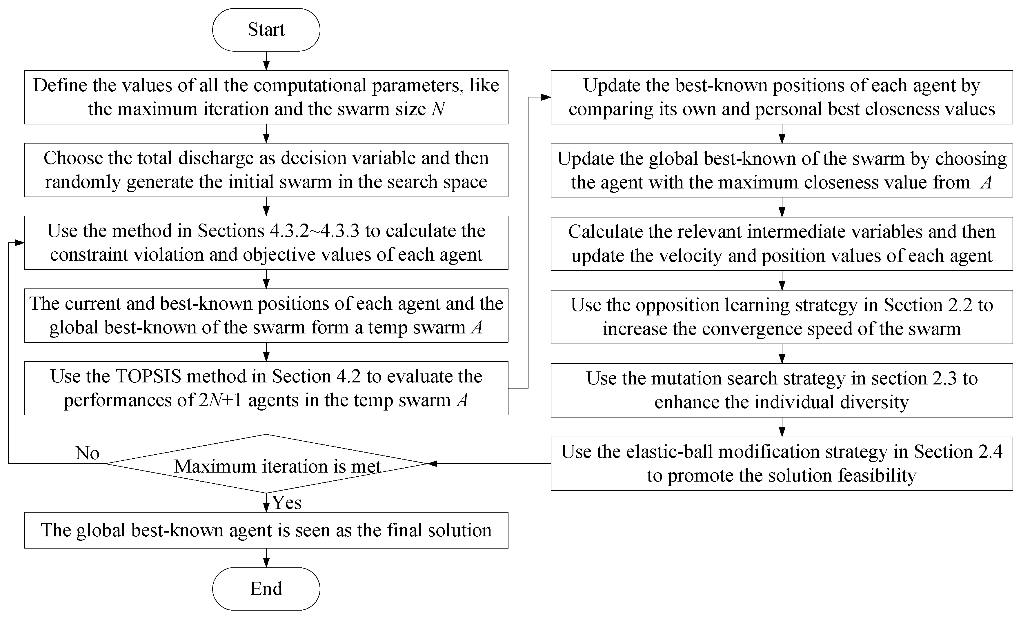
2.5. Execution Procedure of the Proposed EGSA Method

In the EGSA method, three modified strategies (the opposition learning strategy, mutation search strategy, and the elastic-ball modification strategy) were introduced to enhance the global search ability of the standard GSA method in the complex nonlinear constrained optimization problems. Specially, the GSA module could well guarantee the search performance of the swarm; the opposition learning strategy could increase social interaction ability of the agents by exploring the reverse areas; the mutation search strategy was used to balance the convergence speed and the swarm diversity; while the elastic-ball modification strategy could effectively guarantee the feasibility of the newly-generated agents. By combining the advantages of the above strategies, the EGSA method had a stronger ability to enhance the local exploration and global search, in comparison with the conventional GSA method, which would help alleviate the premature convergence problem. Then, the brief execution procedure of the EGSA method was summarized as below:
  • Step 1: Set the values of the computational parameters and then randomly generate the initial swarm in the problem space.
  • Step 2: Calculate the fitness values of all the agents in the current population, and then update the personal best-known of each agent and the global best-known agent of the swarm.
  • Step 3: Calculate the correlated variables (like the gravitational coefficient, mass, and acceleration) to update the velocity and position values of all the agents.
  • Step 4: Execute the opposition learning strategy to increase the convergence speed of the swarm.
  • Step 5: Execute the partial mutation search strategy to enhance the individual diversity.
  • Step 6: Execute the elastic-ball modification strategy to promote the solution feasibility.
  • Step 7: Repeat Step 2–6 until the stopping criterion is met, and then the global optimal position is regarded as the final solution of the optimization problem.

3. Numerical Experiments to Verify the Performance of the EGSA Method

3.1. Benchmark Functions

To verify the performance of the EGSA algorithm, 12 classic benchmark functions are chosen for numerical experiments. Table 1 shows the details of the selected functions, where D is the number of variables; range is the search scope for each variable; and fmin is the optimal objective value in theory. For all test functions, the optimal value of F8, −418.9 × D, varies with the dimension; while the optimal values for other functions are 0. Meanwhile, the benchmark functions are divided into two categories—unimodal functions (F1F8) with one global optimum, and multimodal functions (F9F12) with multiple local optimums. The unimodal functions are used to test the convergence speed of the algorithm, while the multimodal function can test the ability of jumping out of the local optimum, which can fully verify the performance of the evolutionary methods.

3.2. Parameters Settings

For the sake of fair comparison, the results of 11 famous evolutionary algorithms are introduced in this section, including differential evolution (DE), particle swarm optimization (PSO), sine cosine algorithm (SCA), gravitational search algorithm (GSA), ant lion optimizer (ALO) [61], cuckoo search algorithm (CS) [62], modified cuckoo search algorithm (MCS) [63], lightning search algorithm (LSA) [64], grey wolf optimizer (GWO) [65], firefly algorithm (FA) [66], and whale optimization algorithm (WOA) [67]. The results of these five methods (DE, PSO, SCA, GSA, and EGSA) were developed in the JAVA procedures, while the results of the other methods were taken from the corresponding literature. For the five developed methods, the swarm size and maximum iteration were set as 50 and 1000; while the other parameters were set as:
DE: The scaling factor was set as 0.5 and the crossover probability was set as 0.6.
PSO: The inertia weight w was linearly decremented from 0.9 to 0.3; while two learning factors (c1 and c2) were set as 2.0, respectively.
SCA: The computational constant a was set as 2.0.
GSA: The attenuation coefficient was set as 20; the initial gravitational constant was set as 100.
EGSA: The attenuation coefficient was set to 20; the initial gravitational constant was set to 100; while the value of cbest was set to 0.7.

3.3. Comparison with Other Evolutionary Algorithms in Small-Scale Problems

3.3.1. Result Comparison in Multiple Runs

For the sake of alleviating the adverse influence of random initial seeds, all approaches were independently executed 30 times. Table 2 shows the average (Ave.) and standard deviation (Std.) of 12 algorithms for all the test functions, where the number of variables was set as 30. It could be seen that for all the functions, EGSA was always superior to the GSA method in terms of both the average and standard deviation; as compared with other methods, the EGSA method could obtain satisfying results in most functions. For instance, EGSA outperformed ALO in the average of all test functions except for F5, the WOA performance was tied with EGSA in F9 and defeated by EGSA in the other functions. To sum up, the proposed method could obtain better results than the other evolutionary algorithms in the 12 test functions.

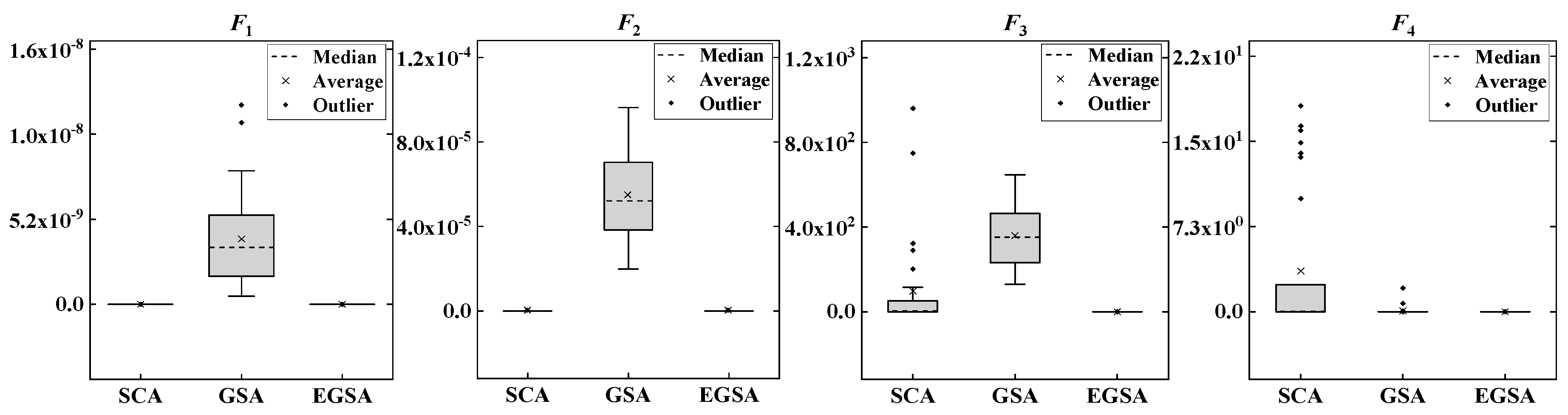
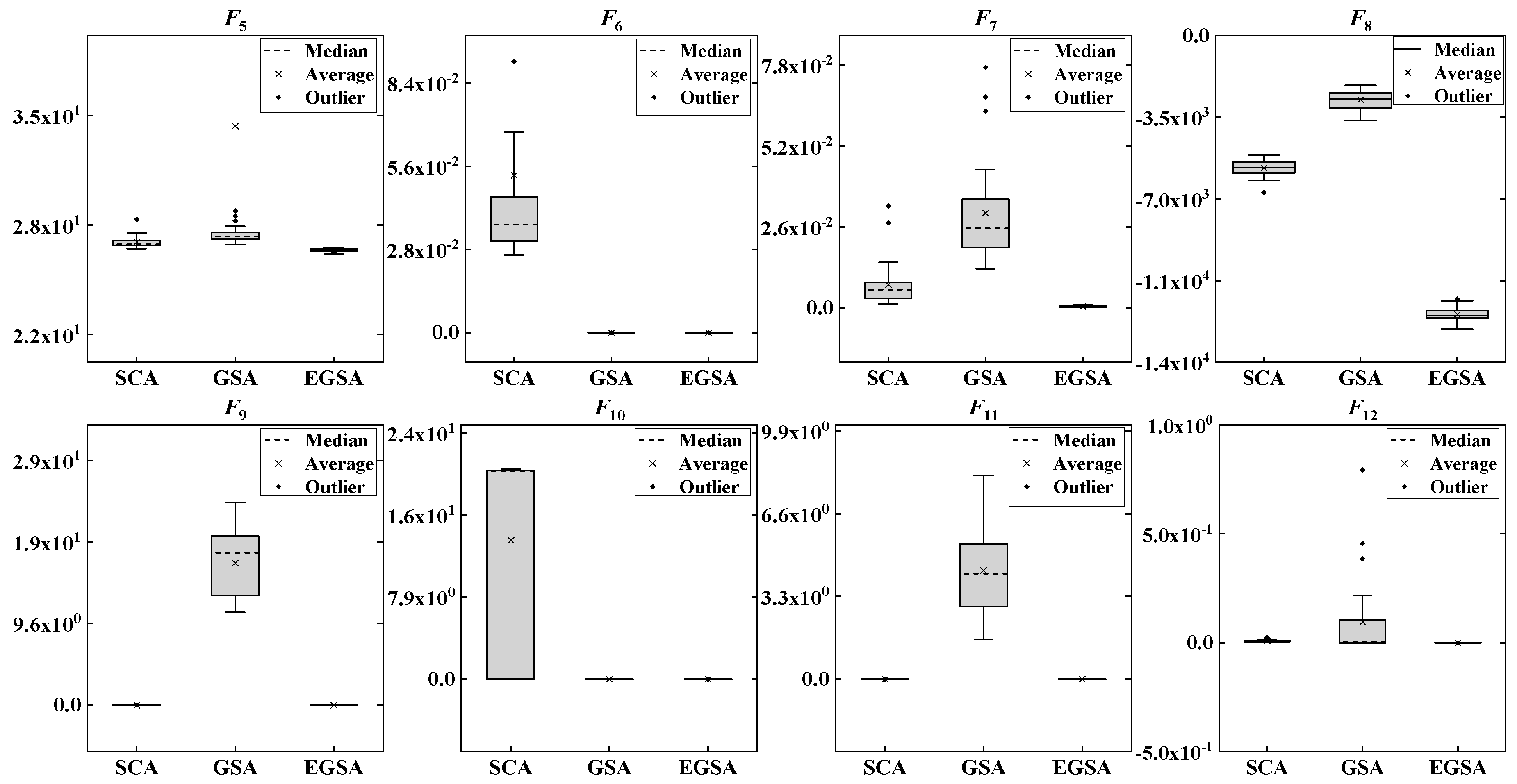
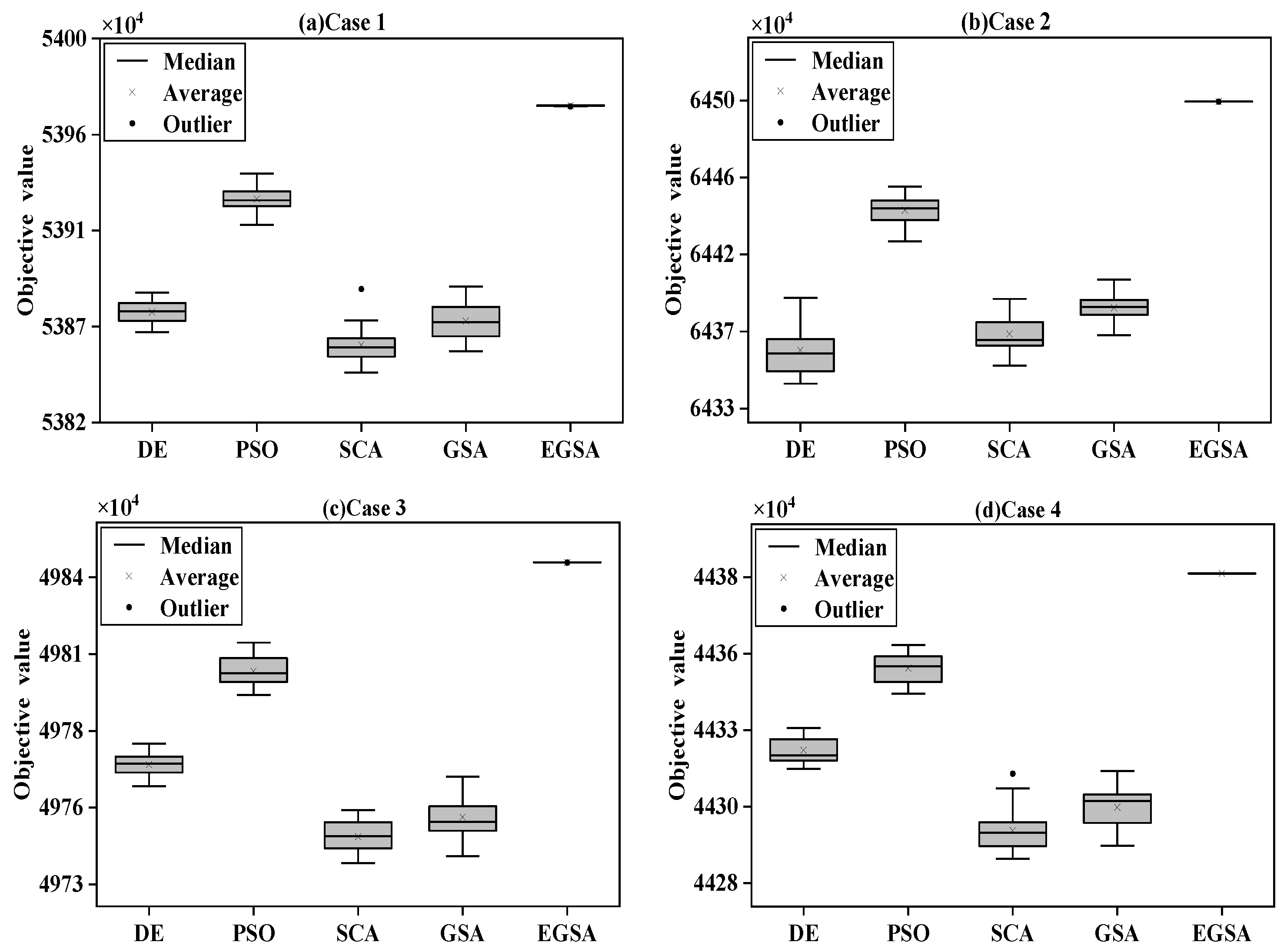
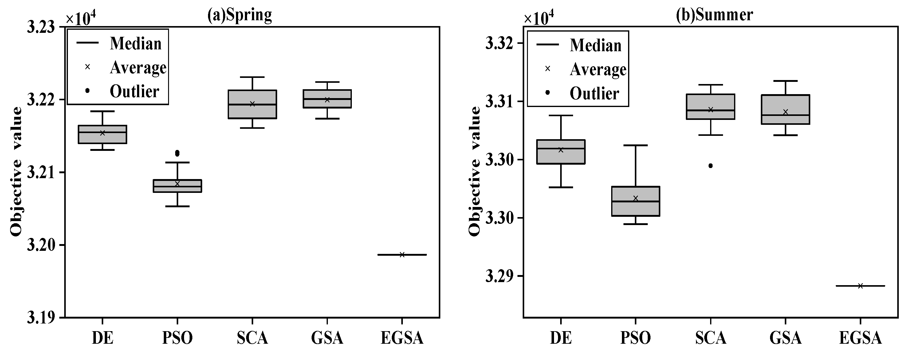
3.3.2. Box and Whisker Test

In this section, the box and whisker test was employed to demonstrate the objective distribution of the solutions since it can show the abundant information (including minimum, second and third quartile, median, and maximum) on the studied data. Figure 2 shows the detailed data obtained by the three methods in 30 independent runs. It could be clearly observed that compared to the other methods, the proposed method had a smaller distribution and better values in all indices. For instance, the standard GSA algorithm had different degrees of outliers on F4F5, which indicated that this method easily fell into the state of premature convergence in the search process; the SCA algorithm exhibited outliers in most functions but had a distribution of relatively discrete solutions in F3, which indicated that SCA was not ideal in terms of robustness. Additionally, the EGSA method had a more concentrated solution distribution and fewer outliers in all functions, demonstrating its satisfying robustness and search ability. Thus, the performances of the EGSA method were superior to the comparative methods in the 12 functions.

3.3.3. Wilcoxon Nonparametric Test

To achieve statistically meaningful conclusions, the Wilcoxon nonparametric test was employed to test the significance level of various methods. Table 3 shows the statistical results of various methods. If the results of the EGSA was better than the control method, it was recorded as a win; if two methods were tied, it was recorded as a tie; otherwise, it was recorded as a loss. From Table 3, it can be seen that the proposed method could produce better solutions as compared to the other methods, due to the larger number of the ‘Win’ symbol. Then, the multiple-problem statistical results obtained by the Wilcoxon nonparametric test with a significance level of 0.05 are given in Table 4, where the mean objective value obtained by each method is chosen as the data sample. From Table 4, it can be found that the proposed method could achieve higher R+ than R in all comparisons, while all values of p were smaller than 0.05. This case proved that the EGSA method outperformed the other methods in a statistical manner.

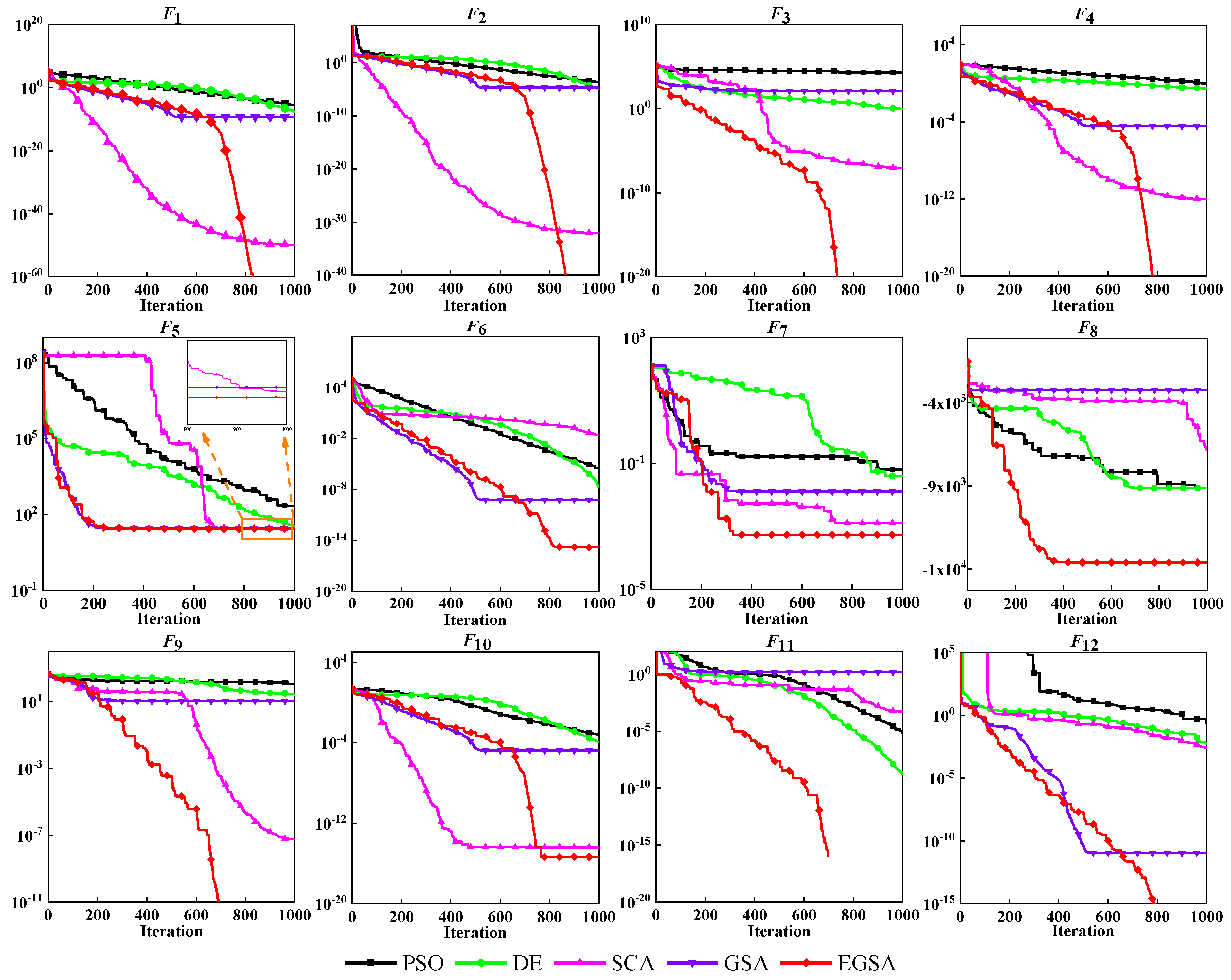
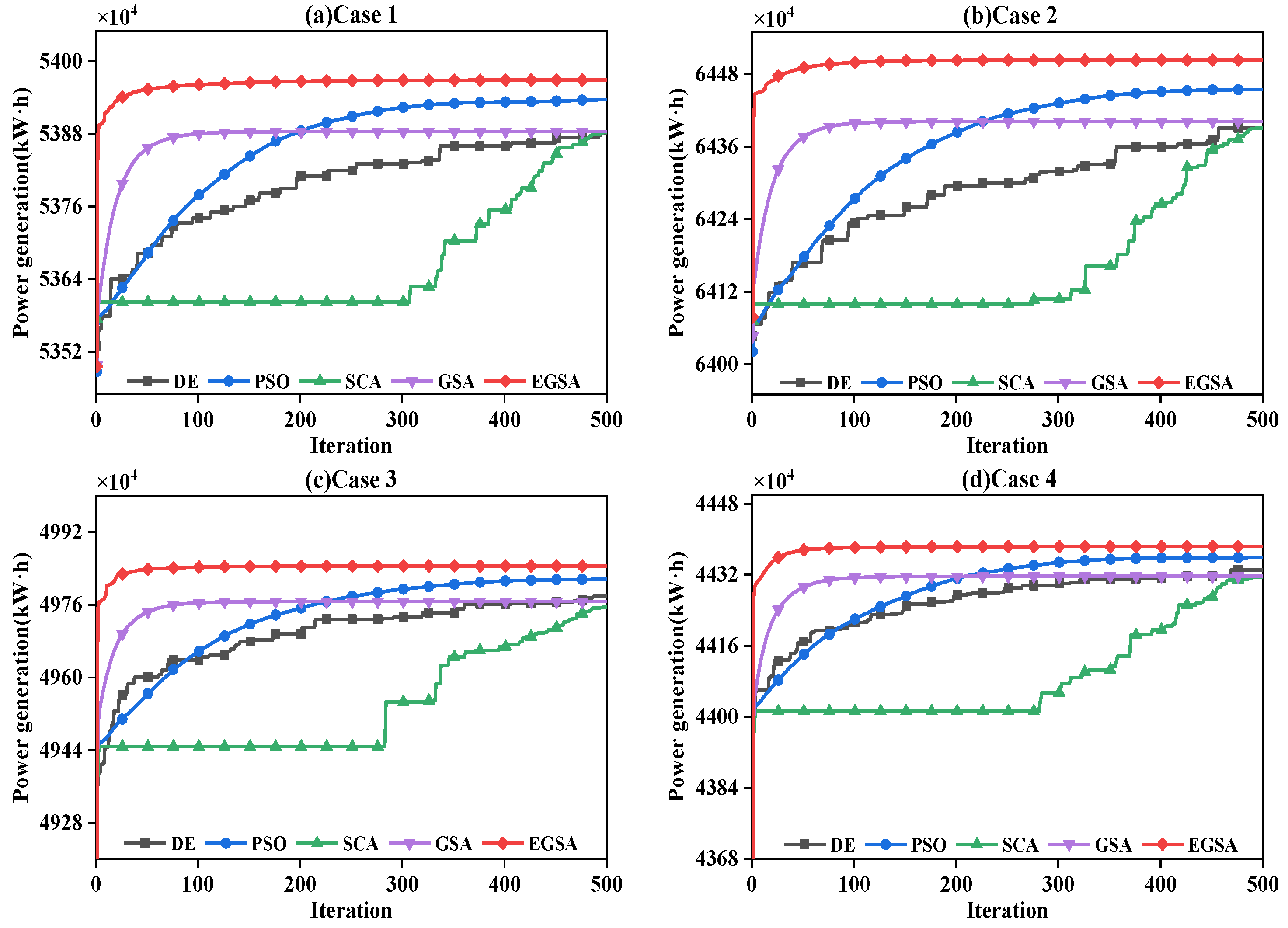
3.3.4. Convergence Analysis

Figure 3 shows the convergence trajectories of five algorithms for 12 functions with 30 variables. It can be seen that the proposed method could constantly improve the solution’s quality from the beginning to the end, and could find the best solutions in the end. Taking the functions F1F4 as examples, three methods (GSA, PSO, and DE) quickly fail into local optima because their best-so-far solutions change slightly in the evolutionary process; both EGSA and SCA converge to a smaller objective at the initial stage, but EGSA can quickly find better solutions at iteration 800, while SCA fails to make it. Additionally, for multimodal functions, EGSAs achieve the global optimal solution in both F9 and F11, and better results than other methods in F8, F10, and F12. Thus, the above analysis fully proves that the presented method has a superior convergence speed and global search ability.

4. EGSA for the Multi-Objective Operation of Cascade Hydropower Reservoirs

4.1. Mathematical Model

4.1.1. Objective Functions

With the advantages of low pollutant emission and high operational efficiency, hydropower now plays an increasingly important role in the energy system throughout the world [68,69,70]. As a result, the cascade hydropower reservoirs are often responsible for a variety of operational requirements. Considering the practical requirements of generation enterprises and electrical power systems in China, the generation benefit and peak operations were chosen as the focus of this paper.
(1) Power Generation
For almost all hydropower enterprises, the economic benefit is an important indicator of performance check under the market environment [71,72,73]. Generally, the same amount of available water resource can produce numerous scheduling schemes with different generation benefits. Hence, the first objective was chosen to find the best scheme that could maximize the total power generation of all hydropower reservoirs, which could be expressed as below:
E = max   t = 1 T n = 1 N P n , t × Δ t
where E is the power generation of all hydropower reservoirs. T is the number of periods. N is the number of hydropower reservoirs. P n , t is the output of the nth hydroplant at the tth period. Δ t is the total hours of the tth period.
(2) Peak Operation
In modern power systems, the hydropower system is often asked to respond to the peak loads of power grid to produce a relatively smooth load series for other kinds of energy systems (like thermal, solar, and wind) [74,75,76]. In this way, the total operational cost of the electrical power system in the long run can be sharply reduced [77,78,79]. Hence, the second objective function was chosen to minimize the mean square deviation of the residual load curve obtained by subtracting all power outputs of hydropower reservoirs from the original energy load curve, which could be expressed as:
F = min   1 2 t = 1 T [ L o a d t n = 1 N P n , t ] 2
where L o a d t is the load demand of the power system at the tth period.

4.1.2. Physical Constraints

(1) Water Balance Equation:
V n , t + 1 = V n , t + 3600 Δ t × [ I n , t + i = 1 N u m ( Q i , t + S i , t ) Q n , t S n , t ]
where V n , t , I n , t , Q n , t , S n , t are the storage volume, local inflow, turbine discharge and spillage of the nth hydroplant at the tth period, respectively. Num is the number of upstream hydroplants directly connected to the nth hydroplant.
(2) Reservoir Storage Constraint:
V _ n , t V n , t V ¯ n , t
where V ¯ n , t and V _ n , t denote the maximum and minimum storage volumes of the nth hydroplant at the tth period, respectively.
(3) Turbine Discharge Constraint:
Q _ n , t Q n , t Q ¯ n , t
where Q ¯ n , t and Q _ n , t denote the maximum and minimum turbine discharges of the nth hydroplant at the tth period, respectively.
(4) Total Discharge Constraint:
q _ n , t q n , t q ¯ n , t
where q ¯ n , t and q _ n , t denote the maximum and minimum total discharges of the nth hydroplant at the tth period, respectively.
(5) Power Output Constraint:
P _ n , t P n , t P ¯ n , t
where P ¯ n , t and P _ n , t denote the maximum and minimum power outputs of the nth hydroplant at the tth period, respectively.
(6) Initial and Final Water Levels Constraint:
{ Z n , 0 = Z n b e g Z n , T = Z n e n d
where Z n b e g and Z n e n d represent the initial and final water level of the nth hydroplant, respectively.

4.2. Technique for Order Preference by Similarity to an Ideal Solution (TOPSIS)

As mentioned above, the multi-objective operation of cascade hydropower reservoirs is a typical multiple-criteria decision-making problem. Thus, it was necessary to find some tools to transform the original multi-objective problem into the single-objective optimization problem that can be addressed by EGSA. After a comprehensive comparison, TOPSIS was introduced to achieve this goal. In TOPSIS, the best scheme had the smallest distance from the positive ideal scheme and the largest distance from the negative ideal scheme, respectively. Then, the procedure of TOPSIS was give as below:
Step 1: Create an initial decision evaluation matrix with m schemes and J attributes. For the target problem, each scheme is composed of two attributes—the power generation E and the peak operation F. Then, the decision-making matrix A can be expressed as follows:
A = ( a i , j ) m × J = [ a 11 a 12 a 1 J a 21 a 22 a 2 J a i , j a m 1 a m 2 a m J ]
where a i , j is the original value of the jth attribute in the ith scheme.
Step 2: Obtain the modified decision evaluation matrix to reduce the potential impact of various attribute properties (like measurement unit and tendency); given below:
B = ( b i , j ) m × J = [ b 11 b 12 b 1 J b 21 b 22 b 2 J b i , j b m 1 b m 2 b m J ]
b i j = { a j max a i j a j max a j min minimization   attribute a i j a j min a j max a j min maximization   attribute , i = 1 , 2 , , m ; j = 1 , 2 , , J
where a j max and a j min are the maximum and minimum values of the jth attribute.
Step 3: Obtain the normalized decision-making matrix to reduce the possible numerical problem caused by the feature differences (like units or magnitude), which could be expressed as below:
R = ( r i , j ) m × J = [ r 11 r 12 r 1 J r 21 r 22 r 2 J r i , j r m 1 r m 2 r m J ]
r i j = b i j i = 1 m b i j 2 , i = 1 , 2 , , m ;   j = 1 , 2 , , J
where r i j is the normalized value of the jth attribute in the ith scheme.
Step 4: Set the weight vector w = [ w 1 , , w j , , w J ] , where w j is the weight of the jth attribute and there is j = 1 J w j = 1 . Then, calculate the weighted normalized decision-making matrix V by:
V = ( v i , j ) m × J = ( w j × r i , j ) m × J
Step 5: Determine the positive ideal scheme C + and negative ideal scheme C by:
{ C + = [ c 1 + , c 2 + , , c J + ] = max { v i , j | i = 1 , 2 , , m } C = [ c 1 , c 2 , , c J ] = min { v i , j | i = 1 , 2 , , m } j = 1 , 2 , , J
Step 6: Calculate the Euclidean distances between the decision scheme and the positive (negative) ideal scheme, which could be expressed as below:
{ D i + = j = 1 J ( v i j c j + ) 2 D i = j = 1 J ( v i j c j ) 2 , i = 1 , 2 , m
where D i + or D i is the distance between the ith scheme and the position (or negative) ideal scheme.
Step 7: Calculate the closeness of each decision plan to the negative ideal scheme by
f i = D i D i + D i + , i = 1 , 2 , m
Step 8: Use the obtained closeness values to sort all the schemes, and the scheme possessing the maximum closeness will be treated as the optimal decision scheme.
f b e s t = max { f 1 , f 2 , , f m }

4.3. Details of EGSA for Multi-Objective Operation of Cascade Hydropower Reservoirs

4.3.1. Individual Structure and Swarm Initialization

To enhance the execution efficiency of reservoir operation, the total discharge of the hydropower reservoir is selected as the decision variable for encoding, and then the ith agent at the kth iteration X i ( k ) can be expressed as below:
X i ( k ) = [ q 1 , 1 q 1 , 2 q 1 , T q 2 , 1 q 2 , 2 q 2 , T q n , t q N , 1 q N , 2 q N , T ]
During the initialization phase, the elements of the solution X i ( k ) are randomly generated in the preset of the total discharge scopes of all hydroplants, which could be expressed as follows:
q n , t = q _ n , t + r a n d o m × ( q ¯ n , t q _ n , t )
where random is the random number uniformly distributed in the range of [0,1].

4.3.2. Heuristic Constraint Handling Method

During the evolutionary process, it is possible that some agents violate the equality or inequality constraints imposed on the hydropower system. In order to effectively modify the infeasible agents, this section presents a heuristic constraint handling method that tries to equally allocate the violated final storage volume to the turbine discharges of all adjusting periods. The detailed procedures for the solution X i ( k ) are given as below:
Step 1: Set n = 1 and determine the necessary parameters for the constraint processing.
Step 2: Set the counter L = 1, and then use the water balance equation to calculate the storage of the nth hydroplant at the tth period by
V n , t = max { V _ n , t , min { V n , t 1 + 3600 Δ t 1 × [ I n , t 1 + i = 1 N u m ( Q i , t 1 + S i , t 1 ) Q n , t 1 S n , t 1 ] , V ¯ n , t } }
Step 3: Set L = L + 1, and then calculate the violation value η n of the final storage by Equation (33). Then, if | η n | is smaller than the accuracy ε or L is larger than the maximum iteration, go to Step 5; otherwise, turn to Step 4.
η n = f n ( Z n , T ) f n ( Z n e n d )
where f n ( · ) is the nonlinear stage-storage curve of the nth hydropower reservoir.
Step 4: Use Equation (34) to obtain the modified total discharges of the target reservoir, and then calculate the corresponding reservoir storage volume by Equation (32) before turning to Step 3.
q n , t = max { q _ n , t , min { q n , t + η n T × 3600 Δ t , q ¯ n , t } }
Step 5: Set n = n+1. If nN, turn to Step 2 for the new hydroplant; otherwise, stop the iteration.

4.3.3. Calculation of the Modified Objective Values

Generally, the agents modified by the above heuristic constraint handling procedures would satisfy most of the physical constraints. Nevertheless, the agents might still violate some constraints due to reasons like unreasonable operation trajectory and limited adjusted times. To eliminate the negative effect of the infeasible agents, the value of the constraint violation involved in the solution X i ( k ) ( V i o l [ X i ( k ) ] for short) was obtained by Equation (35), and then merged into two original objective values (E and F) by Equation (36) to obtain the modified objective values (E and F).
V i o l [ X i ( k ) ] = l 1 = 1 L g c l 1 · max { g l 1 ( X i ( k ) ) , 0 } + l 2 = 1 L e c l 2 · [ e l 2 ( X i ( k ) ) ] 2
{ E [ X i ( k ) ] = t = 1 T n = 1 N P n , t × Δ t V i o l [ X i ( k ) ] F [ X i ( k ) ] = 1 2 t = 1 T [ L o a d t n = 1 N P n , t ] 2 + V i o l [ X i ( k ) ]
where g l 1 ( · ) 0 is the l1th inequality constraint; e l 2 ( · ) 0 is the l2th equality constraint; c l 1 and c l 2 are the penalty coefficients for the relevant inequality or equality constraint. L g and L e denote the number of inequality and equality constraints, respectively.

4.3.4. Execution Procedures of the EGSA Method for the Target Problem

The flowchart of the developed EGSA method for solving multi-objective operation of cascade hydropower reservoirs is given in Figure 4.

5. Case Studies

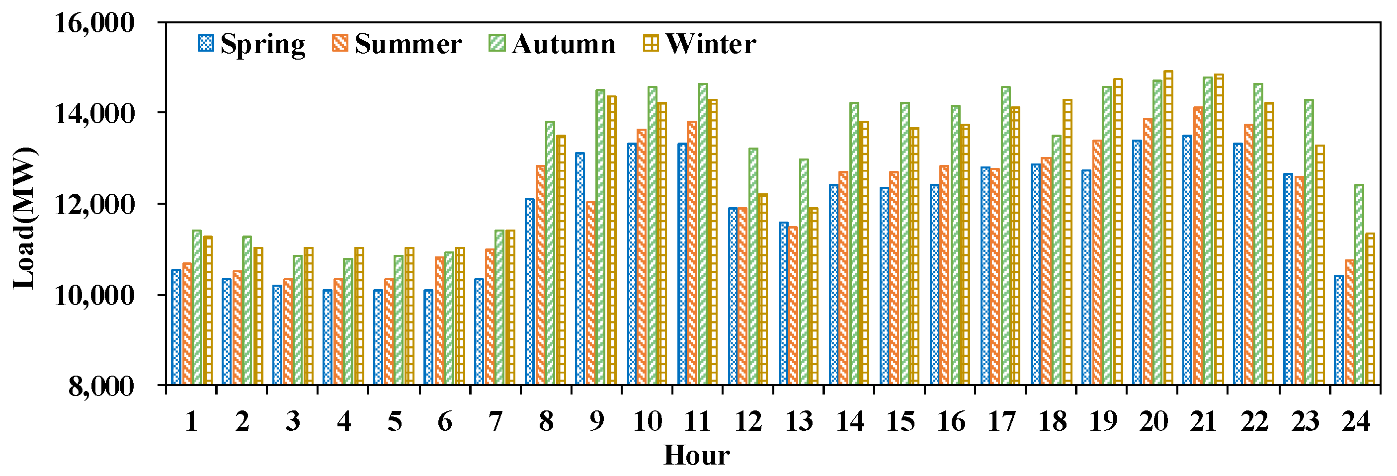
5.1. Engineering Background

In this section, five reservoirs of the Wu hydropower system in Southwest China were chosen to test the performance of the proposed method, including Hongjiadu (HJD), Dongfeng (DF), Suofengying (SFY), Wujiangdu (WJD), and Goupitan (GPT). Since being put into operation, the Wu hydropower system has played a vitally important role in the environment protection and economic development of the Guizhou province. Figure 5 shows the topological structure of the selected hydropower reservoirs, while the typical load demand curves of the four seasons are shown in Figure 6. From Figure 5 and Figure 6, it could be observed that in the Wu hydropower system, there were tight hydraulic and electrical connections from upstream to downstream reservoirs, while four load curves with different features further increased the optimization difficulty.

5.2. Case Study 1: Power Generation of Cascade Hydropower Reservoirs

5.2.1. Robustness Testing of Different Evolutionary Algorithms

In this section, to verify the robustness of the developed method, four famous methods (DE, PSO, SCA, and GSA) were introduced for comparative analysis. Table 5 shows the detailed statistical results of the 5 methods in 20 independent runs for 4 cases, where the swarm size and maximum iteration were set as 50 and 500, respectively. It can be clearly seen that the solutions obtained by the EGSA method were more stable than the other methods. For instance, in Case 1, the EGSA method could make about 96.4%, 96.5%, 97.8%, and 97.7% reductions in the standard deviations of the DE, PSO, SCA, and GSA. Hence, the feasibility of the EGSA method was fully demonstrated in this case.
Figure 7 draws the box and whisker test of the best-so-far solutions obtained by 5 algorithms in 4 cases. It can be observed that the performances of four control methods in the power generation of hydropower system are relatively stable but still inferior to the EGSA method possessing the smallest variation ranges in the final solutions. Therefore, the proposed method proves to be an effective tool to deal with the power generation of a hydropower system.

5.2.2. Comparison of the Optimal Results Obtained by Different Evolutionary Algorithms

Table 6 shows the detailed results in the best solutions obtained by different methods. It can be seen that in all cases, EGSA can always find the best results among all algorithms. For instance, compared with DE, PSO, SCA, and GSA, the EGSA method could make about 8.77 × 10⁴ kW·h, 3.2 × 10⁴ kW·h, 8.61 × 10⁴ kW·h, and 8.5 × 10⁴ kW·h improvements in power generation in Case 1, respectively. Additionally, among all hydroplants, the GPT hydroplant with a huge installed capacity produced the largest proportion of power generation in all solutions, which was in line with the actual operation situation of the hydropower system [80,81,82,83]. Thus, the above analysis demonstrated the effectiveness and rationality of the scheduling process obtained by the proposed method.

5.2.3. Convergence Analysis of Different Evolutionary Algorithms

Figure 8 shows the convergence trajectories of 5 algorithms in different cases. It could be observed that in four cases, SCA failed into a local optima at the early stage, and then started to improve the quality of solutions as the iteration number reached 300, but still failed to find out the satisfying solutions at the end; due to the loss of individual diversity [84], three other methods (PSO, GSA, and DE) outperformed the SCA method but were still inferior to the proposed method from the beginning to end. Additionally, the proposed method could quickly converge to the scheduling schemes that were close to the optimal solution at the early stage, and then change slightly with an increasing number of iterations. Thus, it could be concluded that three modified strategies could effectively enhance the performance of the standard GSA method.

5.3. Case Study 2: Peak Operation of Cascade Hydropower Reservoirs

5.3.1. Robustness Testing of Different Evolutionary Algorithms

In this section, the proposed method was applied to deal with the peak operation of a hydropower system. Table 7 shows the statistical results of the 5 methods in 20 independent runs for 4 cases. It was observed that all of the methods could achieve the goal of reducing the peak loads of a power system due to the reductions in the statistical indices; while the proposed method had the performances among all methods. For instance, the average improvements in the range of the objective values of EGSA was about 99.7%, compared to the three other methods in the 4 cases. Hence, the feasibility of the EGSA method in addressing the peak operation of the hydropower system was proved in this case.
Figure 9 shows the box and whisker test of 5 algorithms in different cases. It can be seen that the distribution ranges of the solutions obtained by the proposed method were much smaller than the other methods, demonstrating the effectiveness of the constraint handling method and the modified strategies. Thus, it can be concluded that the EGSA method could produce stable scheduling schemes for the complex hydropower system peak operation problem.

5.3.2. Comparison of the Optimal Results Obtained by Different Evolutionary Algorithms

To clearly show the feasibility of the EGSA method, the detailed results in the best solutions as obtained by different methods are given in Table 8. It was found that the EGSA method could achieve satisfactory results. For instance, the proposed method could bring about a 30.9% reduction in the peak values in Summer, which was obviously better than 21.0% of DE and 24.9% of PSO, 23.9% of SCA and 19.4% of GSA. Thus, this simulation clearly proved the superiority of the proposed method in responding to the peak operation requirement of the power system.

5.3.3. Rationality Analysis of the Best Results Obtained by the Different Evolutionary Algorithms

Figure 10 shows the detailed output process obtained by the different methods in four cases. It was found that there were often two peak periods (morning and evening) in the original load curves, and obvious differences in the load features (like peak times or numbers) of the four load curves, which would increase the optimization difficulty of the peak operation. The two methods (GSA and EGSA) exhibited excellent responses to the load changes by collecting the hydropower generation at the peak periods and storing the energy at valley periods. The EGSA method was superior to the GSA method due to its smoother residual load curves; besides, the outputs of all the hydroplants varied in the feasible range between the minimum output limit and the installed capacity. Thus, the EGSA method could produce feasible solutions for the peak operation of a hydropower system.

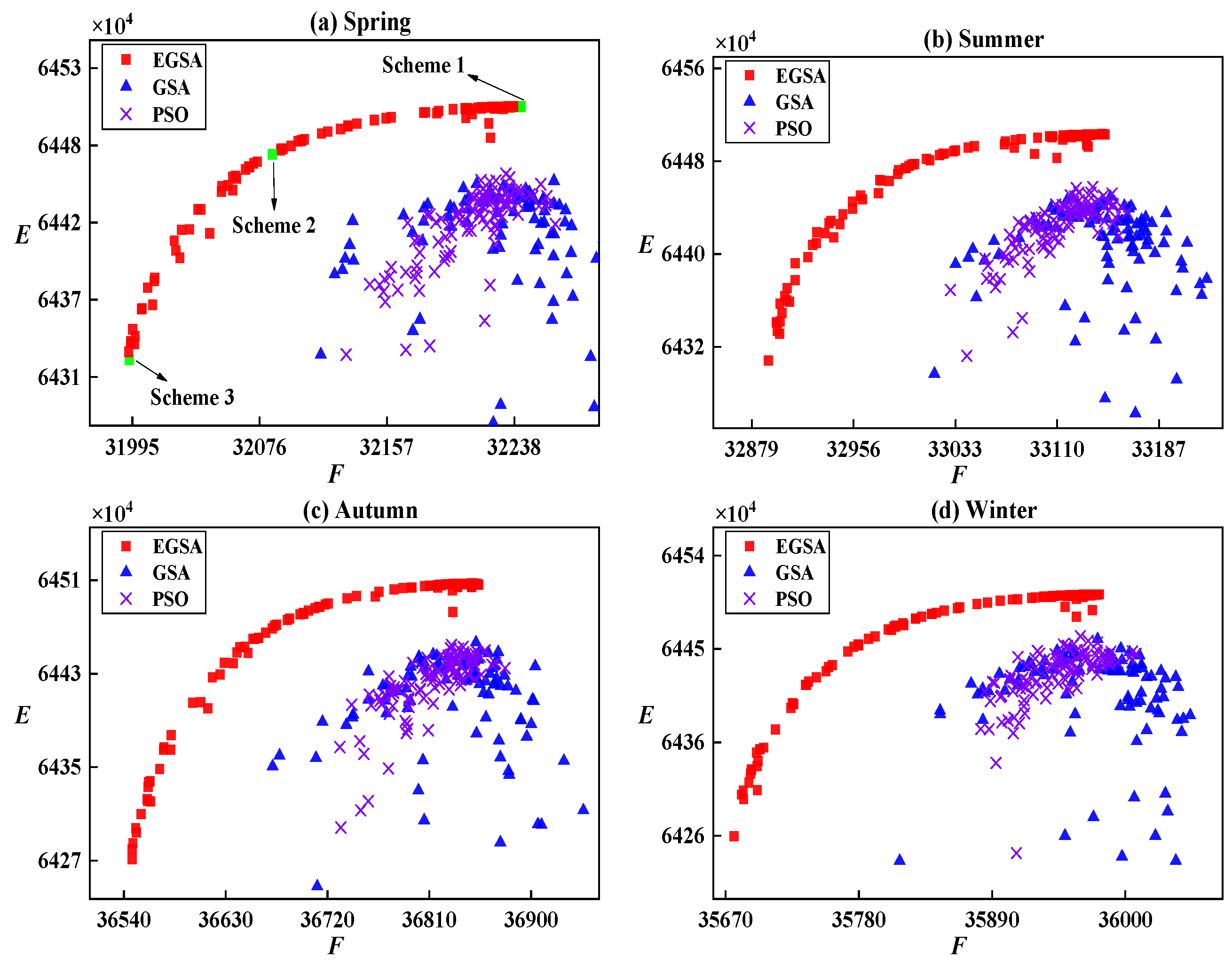
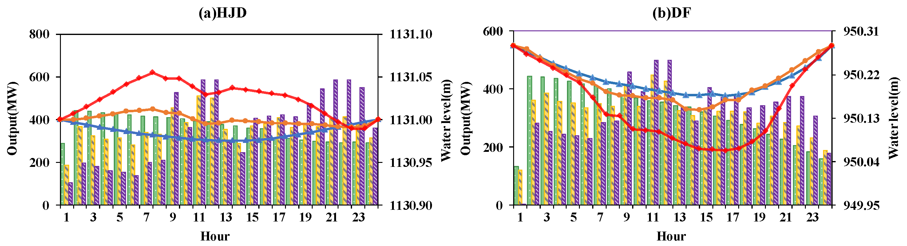
5.4. Case Study 3: Mutli-Objective Operation of Cascade Hydropower Reservoirs

5.4.1. Comparative Analysis of the Optimal Results Obtained by the Different Methods with 100 Weights

The focus of this section is on the demonstration of the feasibility of the proposed method in addressing the multi-objective optimization problems of a hydropower system. Figure 11 draws the distributions of the objective functions obtained by different methods, where each method was executed in 100 different weight combinations. Specifically, the weight w1 for power generation was increased from 0 to 1.0 at the same interval of 0.01, while the weight w2 for peak operation was set as 1.0 – w1. From Figure 11, it was observed that the total generation was gradually decreasing with the increasing objective value of peak operation, which implied that there was an obvious conflict between power generation and peak operation. Additionally, the solutions of PSO and GSA were dominated by that of the EGSA method, which meant that the EGSA method had a higher probability to obtain the Pareto optimal solutions than the PSO and GSA method. Thus, the proposed method can generate the near-optimal Pareto solutions to approximate the relationship between power generation and peak shaving in practice.

5.4.2. Rationality Analysis of the Best Results Obtained by the Different Evolutionary Algorithms

Figure 12 shows the detailed results of three typical schemes obtained by the EGSA method in Spring, where Scheme 1 showed the maximum power generation, Scheme 3 had the best peak operation performance, while Scheme 2 could achieve a balance between power generation and peak operation. It could be seen that for all the hydropower reservoirs, the water levels varied in the preset range between a dead water level and a normal water level while the power outputs were smaller than the installed capacity, demonstrating the effectiveness of the heuristic constraint handling method in guaranteeing the feasibility of the solution. Meanwhile, there were obvious differences in the peak operation and power generations of the three typical schemes, which indicated that it was necessary to choose a suitable scheme based on the actual requirement. Thus, this case again proved the practicability of the EGSA method in solving the multi-objective operation problems.

6. Conclusions

In this research, an enhanced gravitational search algorithm coupled with the Technique for Order Preference by Similarity to an Ideal Solution (TOPSIS) was developed to deal with the complex multi-objective operation problem of cascade hydropower reservoirs balancing the power generation and peak operation benefits. The proposed method and several famous evolutionary methods were used to solve the 12 famous benchmark functions and the optimal operation of the Wu hydropower system in China. The critical findings obtained from the experimental results are given as below:
(1)
Due to the loss of the population diversity, the conventional GSA method suffered from severe premature convergence shortcomings. The proposed method based on the three modified strategies (opposite learning strategy, partial mutation strategy and elastic-ball modification strategy) could effectively improve the convergence speed, swarm diversity, and solution feasibility of the standard GSA method, respectively.
(2)
For the original complex multi-objective optimization problem, balancing power generation and peak operation requirements, the famous TOPSIS method was used to transform it into the relatively simple single-objective problem, which could help make an obvious reduction in the modeling difficulty of the multi-objective decision.
(3)
There was a competitive relationship between the generation benefit of the hydropower enterprise and the peak operation of the power system. In other words, an increasing value of one objective would obviously reduce another objective value. Thus, it was necessary for operators to carefully determine the scheduling schemes so as to effectively balance the practical requirements of power generation enterprises and power grid companies.

Author Contributions

All authors contributed extensively to the work presented in this paper. Z.-k.F. and W.-j.N. contributed to the finalized the manuscripts. S.L. contributed to the modeling and programming. Z.-q.J. contributed to the literature review. M.-s.M. and B.L. contributed to the data analyses.

Funding

This research was supported by the Natural Science Foundation of Hubei Province (2018CFB573), National Natural Science Foundation of China (51709119 and 51909133), and the Fundamental Research Funds for the Central Universities (HUST: 2017KFYXJJ193).

Acknowledgments

The writers would like to express appreciation to both editors and reviewers for their valuable comments and suggestions.

Conflicts of Interest

The authors declare no conflict of interest.

References

  1. Chang, J.; Li, Y.; Yuan, M.; Wang, Y. Efficiency evaluation of hydropower station operation: A case study of Longyangxia station in the Yellow River, China. Energy 2017, 135, 23–31. [Google Scholar] [CrossRef]
  2. Feng, M.; Liu, P.; Guo, S.; Gui, Z.; Zhang, X.; Zhang, W.; Xiong, L. Identifying changing patterns of reservoir operating rules under various inflow alteration scenarios. Adv. Water Resour. 2017, 104, 23–36. [Google Scholar] [CrossRef]
  3. Liu, P.; Li, L.; Chen, G.; Rheinheimer, D.E. Parameter uncertainty analysis of reservoir operating rules based on implicit stochastic optimization. J. Hydrol. 2014, 514, 102–113. [Google Scholar] [CrossRef]
  4. Zhao, T.; Zhao, J.; Yang, D. Improved dynamic programming for hydropower reservoir operation. J. Water Res. Plan. Manag. 2014, 140, 365–374. [Google Scholar] [CrossRef]
  5. Liu, S.; Feng, Z.K.; Niu, W.J.; Zhang, H.R.; Song, Z.G. Peak operation problem solving for hydropower reservoirs by elite-guide sine cosine algorithm with Gaussian local search and random mutation. Energies 2019, 12, 2189. [Google Scholar] [CrossRef]
  6. Feng, Z.K.; Niu, W.J.; Cheng, C.T. China’s large-scale hydropower system: Operation characteristics, modeling challenge and dimensionality reduction possibilities. Renew. Energy 2019, 136, 805–818. [Google Scholar] [CrossRef]
  7. Bai, T.; Wu, L.; Chang, J.X.; Huang, Q. Multi-Objective Optimal Operation Model of Cascade Reservoirs and Its Application on Water and Sediment Regulation. Water Resour. Manag. 2015, 29, 2751–2770. [Google Scholar] [CrossRef]
  8. Guo, X.Y.; Ma, C.; Tang, Z.B. Multi-timescale joint optimal dispatch model considering environmental flow requirements for a dewatered river channel: Case study of Jinping cascade hydropower stations. J. Water Res. Plan. Manag. 2018, 144, 05018014. [Google Scholar] [CrossRef]
  9. Liu, P.; Nguyen, T.D.; Cai, X.; Jiang, X. Finding multiple optimal solutions to optimal load distribution problem in hydropower plant. Energies 2012, 5, 1413–1432. [Google Scholar] [CrossRef]
  10. Chang, J.; Wang, X.; Li, Y.; Wang, Y.; Zhang, H. Hydropower plant operation rules optimization response to climate change. Energy 2018, 160, 886–897. [Google Scholar] [CrossRef]
  11. Guo, S.; Chen, J.; Li, Y.; Liu, P.; Li, T. Joint operation of the multi-reservoir system of the Three Gorges and the Qingjiang cascade reservoirs. Energies 2011, 4, 1036–1050. [Google Scholar] [CrossRef]
  12. Zhang, Y.; Jiang, Z.; Ji, C.; Sun, P. Contrastive analysis of three parallel modes in multi-dimensional dynamic programming and its application in cascade reservoirs operation. J. Hydrol. 2015, 529, 22–34. [Google Scholar] [CrossRef]
  13. Reddy, S.; Abhyankar, A.R.; Bijwe, P.R. Reactive power price clearing using multi-objective optimization. Energy 2011, 36, 3579–3589. [Google Scholar] [CrossRef]
  14. Feng, Z.K.; Niu, W.J.; Wang, S.; Cheng, C.T.; Jiang, Z.Q.; Qin, H.; Liu, Y. Developing a successive linear programming model for head-sensitive hydropower system operation considering power shortage aspect. Energy 2018, 155, 252–261. [Google Scholar] [CrossRef]
  15. Catalao, J.P.S.; Mariano, S.J.P.S.; Mendes, V.M.F.; Ferreira, L.A.F.M. Scheduling of head-sensitive cascaded hydro systems: A nonlinear approach. IEEE Trans. Power Syst. 2009, 24, 337–346. [Google Scholar] [CrossRef]
  16. Jiang, Z.; Wang, C.; Liu, Y.; Feng, Z.; Ji, C.; Zhang, H. Study on the raw water allocation and optimization in shenzhen city, China. Water 2019, 11, 1426. [Google Scholar] [CrossRef]
  17. Jiang, Z.; Ji, C.; Qin, H.; Feng, Z. Multi-stage progressive optimality algorithm and its application in energy storage operation chart optimization of cascade reservoirs. Energy 2018, 148, 309–323. [Google Scholar] [CrossRef]
  18. Huang, G.H.; He, L.; Zeng, G.M.; Lu, H.W. Identification of optimal urban solid waste flow schemes under impacts of energy prices. Environ. Eng. Sci. 2008, 25, 685–695. [Google Scholar] [CrossRef]
  19. Ren, G.; Cao, Y.; Wen, S.; Huang, T.; Zeng, Z. A modified Elman neural network with a new learning rate scheme. Neurocomputing 2018, 286, 11–18. [Google Scholar] [CrossRef]
  20. Xie, X.; Wen, S.; Zeng, Z.; Huang, T. Memristor-based circuit implementation of pulse-coupled neural network with dynamical threshold generators. Neurocomputing 2018, 284, 10–16. [Google Scholar] [CrossRef]
  21. Wen, S.; Xie, X.; Yan, Z.; Huang, T.; Zeng, Z. General memristor with applications in multilayer neural networks. Neural Netw. 2018, 103, 142–149. [Google Scholar] [CrossRef] [PubMed]
  22. Yang, T.; Gao, X.; Sellars, S.L.; Sorooshian, S. Improving the multi-objective evolutionary optimization algorithm for hydropower reservoir operations in the California Oroville-Thermalito complex. Environ. Model. Softw. 2015, 69, 262–279. [Google Scholar] [CrossRef]
  23. Xu, B.; Zhong, P.A.; Du, B.; Chen, J.; Liu, W.; Li, J.; Guo, L.; Zhao, Y. Analysis of a stochastic programming model for optimal hydropower system operation under a deregulated electricity market by considering forecasting uncertainty. Water 2018, 10, 885. [Google Scholar] [CrossRef]
  24. Zhao, T.; Zhao, J. Improved multiple-objective dynamic programming model for reservoir operation optimization. J. Hydroinform. 2014, 16, 1142–1157. [Google Scholar] [CrossRef]
  25. Feng, Z.K.; Niu, W.J.; Cheng, C.T. Optimizing electrical power production of hydropower system by uniform progressive optimality algorithm based on two-stage search mechanism and uniform design. J. Clean. Prod. 2018, 190, 432–442. [Google Scholar] [CrossRef]
  26. Catalão, J.P.S.; Mariano, S.J.P.S.; Mendes, V.M.F.; Ferreira, L.A.F.M. Nonlinear optimization method for short-term hydro scheduling considering head-dependency. Eur. Trans. Electr. Power 2010, 20, 172–183. [Google Scholar] [CrossRef]
  27. Jia, B.; Zhong, P.; Wan, X.; Xu, B.; Chen, J. Decomposition-coordination model of reservoir group and flood storage basin for real-time flood control operation. Hydrol. Res. 2015, 46, 11–25. [Google Scholar] [CrossRef]
  28. Dong, M.; Wen, S.; Zeng, Z.; Yan, Z.; Huang, T. Sparse fully convolutional network for face labeling. Neurocomputing 2019, 331, 465–472. [Google Scholar] [CrossRef]
  29. Li, Z.; Dong, M.; Wen, S.; Hu, X.; Zhou, P.; Zeng, Z. CLU-CNNs: Object detection for medical images. Neurocomputing 2019, 350, 53–59. [Google Scholar] [CrossRef]
  30. Cao, Y.; Wang, S.; Guo, Z.; Huang, T.; Wen, S. Synchronization of memristive neural networks with leakage delay and parameters mismatch via event-triggered control. Neural Netw. 2019, 119, 178–189. [Google Scholar] [CrossRef]
  31. Zheng, F. Comparing the real-time searching behavior of four differential-evolution variants applied to water-distribution-network design optimization. J. Water Res. Plan. Manag. 2015, 141, 04015016. [Google Scholar] [CrossRef]
  32. Yang, T.; Asanjan, A.A.; Faridzad, M.; Hayatbini, N.; Gao, X.; Sorooshian, S. An enhanced artificial neural network with a shuffled complex evolutionary global optimization with principal component analysis. Inf. Sci. 2017, 418–419, 302–316. [Google Scholar] [CrossRef]
  33. Wan, W.; Guo, X.; Lei, X.; Jiang, Y.; Wang, H. A Novel Optimization Method for Multi-Reservoir Operation Policy Derivation in Complex Inter-Basin Water Transfer System. Water Resour. Manag. 2018, 32, 31–51. [Google Scholar] [CrossRef]
  34. Feng, Z.K.; Niu, W.J.; Cheng, C.T. Optimization of hydropower reservoirs operation balancing generation benefit and ecological requirement with parallel multi-objective genetic algorithm. Energy 2018, 153, 706–718. [Google Scholar] [CrossRef]
  35. Zheng, F.; Zecchin, A.C.; Maier, H.R.; Simpson, A.R. Comparison of the searching behavior of NSGA-II, SAMODE, and borg MOEAs applied to water distribution system design problems. J. Water Res. Plan. Manag. 2016, 142, 04016017. [Google Scholar] [CrossRef]
  36. Salkuti, S.R. Short-term electrical load forecasting using hybrid ANN–DE and wavelet transforms approach. Electr. Eng. 2018, 100, 2755–2763. [Google Scholar] [CrossRef]
  37. Chang, J.X.; Bai, T.; Huang, Q.; Yang, D.W. Optimization of Water Resources Utilization by PSO-GA. Water Resour. Manag. 2013, 27, 3525–3540. [Google Scholar] [CrossRef]
  38. Ji, Y.; Lei, X.; Cai, S.; Wang, X. Hedging rules for water supply reservoir based on the model of simulation and optimization. Water 2016, 8, 249. [Google Scholar] [CrossRef]
  39. Zhang, J.; Li, Z.; Wang, X.; Lei, X.; Liu, P.; Feng, M.; Khu, S.T.; Wang, H. A novel method for deriving reservoir operating rules based on flood classification-aggregation-decomposition. J. Hydrol. 2019, 568, 722–734. [Google Scholar] [CrossRef]
  40. Niu, W.J.; Feng, Z.K.; Cheng, C.T.; Wu, X.Y. A parallel multi-objective particle swarm optimization for cascade hydropower reservoir operation in southwest China. Appl. Soft Comput. J. 2018, 70, 562–575. [Google Scholar] [CrossRef]
  41. Ming, B.; Chang, J.X.; Huang, Q.; Wang, Y.M.; Huang, S.Z. Optimal Operation of Multi-Reservoir System Based-On Cuckoo Search Algorithm. Water Resour. Manag. 2015, 29, 5671–5687. [Google Scholar] [CrossRef]
  42. Reddy, S.S.; Panigrahi, B.K.; Debchoudhury, S.; Kundu, R.; Mukherjee, R. Short-term hydro-thermal scheduling using CMA-ES with directed target to best perturbation scheme. Int. J. Bio-Inspired Comput. 2015, 7, 195–208. [Google Scholar] [CrossRef]
  43. Salkuti, S.R. Short-term optimal hydro-thermal scheduling using clustered adaptive teaching learning based optimization. Int. J. Electr. Comput. Eng. 2019, 9, 3359–3365. [Google Scholar]
  44. Niu, W.; Feng, Z.; Cheng, C.; Zhou, J. Forecasting daily runoff by extreme learning machine based on quantum-behaved particle swarm optimization. J. Hydrol. Eng. 2018, 23, 04018002. [Google Scholar] [CrossRef]
  45. Zheng, F.; Zecchin, A.C.; Simpson, A.R. Self-adaptive differential evolution algorithm applied to water distribution system optimization. J. Comput. Civ. Eng. 2013, 27, 148–158. [Google Scholar] [CrossRef]
  46. Zheng, F.; Simpson, A.R.; Zecchin, A.C. A combined NLP-differential evolution algorithm approach for the optimization of looped water distribution systems. Water Resour. Res. 2011, 47. [Google Scholar] [CrossRef] [Green Version]
  47. Feng, Z.K.; Niu, W.J.; Cheng, C.T. Multi-objective quantum-behaved particle swarm optimization for economic environmental hydrothermal energy system scheduling. Energy 2017, 131, 165–178. [Google Scholar] [CrossRef]
  48. Bai, T.; Kan, Y.B.; Chang, J.X.; Huang, Q.; Chang, F.J. Fusing feasible search space into PSO for multi-objective cascade reservoir optimization. Appl. Soft Comput. J. 2017, 51, 328–340. [Google Scholar] [CrossRef]
  49. Rezaei, F.; Safavi, H.R.; Mirchi, A.; Madani, K. f-MOPSO: An alternative multi-objective PSO algorithm for conjunctive water use management. J. Hydro-Environ. Res. 2017, 14, 1–18. [Google Scholar] [CrossRef]
  50. Reddy, S.S.; Bijwe, P.R. Multi-Objective Optimal Power Flow Using Efficient Evolutionary Algorithm. Int. J. Emerg. Electr. Power Syst. 2017, 18. [Google Scholar] [CrossRef]
  51. Ji, B.; Yuan, X.; Yuan, Y.; Lei, X.; Fernando, T.; Iu, H.H.C. Exact and heuristic methods for optimizing lock-quay system in inland waterway. Eur. J. Oper. Res. 2019, 277, 740–755. [Google Scholar] [CrossRef]
  52. Mirjalili, S.; Lewis, A. Adaptive gbest-guided gravitational search algorithm. Neural Comput. Appl. 2014, 25, 1569–1584. [Google Scholar] [CrossRef]
  53. Rashedi, E.; Nezamabadi-Pour, H.; Saryazdi, S. GSA: A gravitational search algorithm. Inf. Sci. 2009, 179, 2232–2248. [Google Scholar] [CrossRef]
  54. Niu, W.J.; Feng, Z.K.; Zeng, M.; Feng, B.F.; Min, Y.W.; Cheng, C.T.; Zhou, J.Z. Forecasting reservoir monthly runoff via ensemble empirical mode decomposition and extreme learning machine optimized by an improved gravitational search algorithm. Appl. Soft Comput. J. 2019, 82, 105589. [Google Scholar] [CrossRef]
  55. Tian, H.; Yuan, X.; Ji, B.; Chen, Z. Multi-objective optimization of short-term hydrothermal scheduling using non-dominated sorting gravitational search algorithm with chaotic mutation. Energy Convers. Manag. 2014, 81, 504–519. [Google Scholar] [CrossRef]
  56. Mahootchi, M.; Tizhoosh, H.R.; Ponnambalam, K. Oppositional extension of reinforcement learning techniques. Inf. Sci. 2014, 275, 101–114. [Google Scholar] [CrossRef]
  57. Mahdavi, S.; Rahnamayan, S.; Deb, K. Opposition based learning: A literature review. Swarm Evol. Comput. 2018, 39, 1–23. [Google Scholar] [CrossRef]
  58. Ewees, A.A.; Abd Elaziz, M.; Houssein, E.H. Improved grasshopper optimization algorithm using opposition-based learning. Expert Syst. Appl. 2018, 112, 156–172. [Google Scholar] [CrossRef]
  59. Xia, Y.; Feng, Z.; Niu, W.; Qin, H.; Jiang, Z.; Zhou, J. Simplex quantum-behaved particle swarm optimization algorithm with application to ecological operation of cascade hydropower reservoirs. Appl. Soft Comput. 2019, 84, 105715. [Google Scholar] [CrossRef]
  60. Chen, Z.; Yuan, X.; Tian, H.; Ji, B. Improved gravitational search algorithm for parameter identification of water turbine regulation system. Energy Convers. Manag. 2014, 78, 306–315. [Google Scholar] [CrossRef]
  61. Mirjalili, S. The ant lion optimizer. Adv. Eng. Softw. 2015, 83, 80–98. [Google Scholar] [CrossRef]
  62. Yang, X.; Deb, S. Cuckoo Search via Lévy Flights; IEEE: Piscataway, NJ, USA, 2009; pp. 210–214. [Google Scholar]
  63. Walton, S.; Hassan, O.; Morgan, K.; Brown, M.R. Modified cuckoo search: A new gradient free optimisation algorithm. Chaos Solitons Fractals 2011, 44, 710–718. [Google Scholar] [CrossRef]
  64. Shareef, H.; Ibrahim, A.A.; Mutlag, A.H. Lightning search algorithm. Appl. Soft Comput. 2015, 36, 315–333. [Google Scholar] [CrossRef]
  65. Mirjalili, S.; Mirjalili, S.M.; Lewis, A. Grey wolf optimizer. Adv. Eng. Softw. 2014, 69, 46–61. [Google Scholar] [CrossRef]
  66. Yang, X.S. Firefly Algorithm in Engineering Optimization; John Wiley & Sons Inc.: Hoboken, NJ, USA, 2010. [Google Scholar]
  67. Mirjalili, S.; Lewis, A. The whale optimization algorithm. Adv. Eng. Softw. 2016, 95, 51–67. [Google Scholar] [CrossRef]
  68. Hua, Z.; Ma, C.; Lian, J.; Pang, X.; Yang, W. Optimal capacity allocation of multiple solar trackers and storage capacity for utility-scale photovoltaic plants considering output characteristics and complementary demand. Appl. Energy 2019, 238, 721–733. [Google Scholar] [CrossRef]
  69. Reddy, S.S.; Bijwe, P.R.; Abhyankar, A.R. Optimal dynamic emergency reserve activation using spinning, hydro and demand-side reserves. Front. Energy 2016, 10, 409–423. [Google Scholar] [CrossRef]
  70. Reddy, S.S.; Bijwe, P.R. Real time economic dispatch considering renewable energy resources. Renew. Energy 2015, 83, 1215–1226. [Google Scholar] [CrossRef]
  71. Feng, Z.K.; Niu, W.J.; Zhang, R.; Wang, S.; Cheng, C.T. Operation rule derivation of hydropower reservoir by k-means clustering method and extreme learning machine based on particle swarm optimization. J. Hydrol. 2019, 576, 229–238. [Google Scholar] [CrossRef]
  72. Feng, Z.K.; Niu, W.J.; Cheng, C.T.; Wu, X.Y. Optimization of hydropower system operation by uniform dynamic programming for dimensionality reduction. Energy 2017, 134, 718–730. [Google Scholar] [CrossRef]
  73. Zhang, C.; Ding, W.; Li, Y.; Meng, F.; Fu, G. Cost-Benefit Framework for Optimal Design of Water Transfer Systems. J. Water Res. Plan. Manag. 2019, 145, 04019007. [Google Scholar] [CrossRef]
  74. Li, H.; Chen, D.; Arzaghi, E.; Abbassi, R.; Xu, B.; Patelli, E.; Tolo, S. Safety assessment of hydro-generating units using experiments and grey-entropy correlation analysis. Energy 2018, 165, 222–234. [Google Scholar] [CrossRef] [Green Version]
  75. Chen, D.; Liu, S.; Ma, X. Modeling, nonlinear dynamical analysis of a novel power system with random wind power and it’s control. Energy 2013, 53, 139–146. [Google Scholar] [CrossRef]
  76. Zhang, R.; Chen, D.; Ma, X. Nonlinear predictive control of a hydropower system model. Entropy-Switz 2015, 17, 6129–6149. [Google Scholar] [CrossRef]
  77. Feng, Z.; Niu, W.; Wang, W.; Zhou, J.; Cheng, C. A mixed integer linear programming model for unit commitment of thermal plants with peak shaving operation aspect in regional power grid lack of flexible hydropower energy. Energy 2019, 175, 618–629. [Google Scholar] [CrossRef]
  78. Feng, Z.; Niu, W.; Wang, S.; Cheng, C.; Song, Z. Mixed integer linear programming model for peak operation of gas-fired generating units with disjoint-prohibited operating zones. Energies 2019, 12, 2179. [Google Scholar] [CrossRef]
  79. Feng, Z.K.; Niu, W.J.; Cheng, C.T.; Zhou, J.Z. Peak shaving operation of hydro-thermal-nuclear plants serving multiple power grids by linear programming. Energy 2017, 135, 210–219. [Google Scholar] [CrossRef]
  80. Niu, W.J.; Feng, Z.K.; Feng, B.F.; Min, Y.W.; Cheng, C.T.; Zhou, J.Z. Comparison of multiple linear regression, artificial neural network, extreme learning machine, and support vector machine in deriving operation rule of hydropower reservoir. Water 2019, 11, 88. [Google Scholar] [CrossRef]
  81. Ma, C.; Lian, J.; Wang, J. Short-term optimal operation of Three-gorge and Gezhouba cascade hydropower stations in non-flood season with operation rules from data mining. Energy Convers. Manag. 2013, 65, 616–627. [Google Scholar] [CrossRef]
  82. Jiang, Z.; Liu, P.; Ji, C.; Zhang, H.; Chen, Y. Ecological flow considered multi-objective sorage energy operation chart optimization of large-scale mixed reservoirs. J. Hydrol. 2019, 577, 123949. [Google Scholar] [CrossRef]
  83. Lian, J.; Yao, Y.; Ma, C.; Guo, Q. Reservoir operation rules for controlling algal blooms in a tributary to the impoundment of three Gorges Dam. Water 2014, 6, 3200–3223. [Google Scholar] [CrossRef]
  84. Fu, W.; Wang, K.; Zhang, C.; Tan, J. A hybrid approach for measuring the vibrational trend of hydroelectric unit with enhanced multi-scale chaotic series analysis and optimized least squares support vector machine. Trans. Inst. Meas. Control 2019, 41, 4436–4449. [Google Scholar] [CrossRef]
Figure 1. Sketch map of the gravitational search algorithm (GSA) method for a two-variable problem.
Water 11 02040 g001
Figure 2. Box and whisker test of three algorithms for 12 functions with 30 variables.
Water 11 02040 g002aWater 11 02040 g002b
Figure 3. Convergence trajectories of the different methods for 12 benchmark functions with 30 variables.
Water 11 02040 g003
Figure 4. The flowchart of enhanced gravitational search algorithm (EGSA) for multi-objective operation of cascade hydropower reservoirs.
Water 11 02040 g004
Figure 5. The topological structure of the studied hydropower reservoirs.
Water 11 02040 g005
Figure 6. Typical load curves in different season.
Water 11 02040 g006
Figure 7. Box and whisker test of different algorithms in different cases for power generation.
Water 11 02040 g007
Figure 8. Convergence trajectories of 5 methods in different cases.
Water 11 02040 g008
Figure 9. Box and whisker test of 5 algorithms in different cases for peak operation.
Water 11 02040 g009aWater 11 02040 g009b
Figure 10. Detailed output process obtained by the different methods in the four cases.
Water 11 02040 g010
Figure 11. Distributions of the objective functions obtained by different methods with 100 weights.
Water 11 02040 g011
Figure 12. Detailed scheduling results of three typical schemes obtained by EGSA in Spring.
Water 11 02040 g012aWater 11 02040 g012b
Table 1. Detailed information of the twelve benchmark functions.
FunctionDRangefmin
F 1 ( x ) = i = 1 n x i 2 30[−100,100]0
F 2 ( x ) = i = 1 n | x i | + i = 1 n | x i | 30[−10,10]0
F 3 ( x ) = i = 1 n ( j = 1 i x j ) 2 30[−100,100]0
F 4 ( x ) = max { | x i | , 1 i n } 30[−100,100]0
F 5 ( x ) = i = 1 n 1 [ 100 ( x i + 1 x i 2 ) 2 + ( x i 1 ) 2 ] 30[−30,30]0
F 6 ( x ) = i = 1 n ( x i + 0.5 ) 2 30[−100,100]0
F 7 ( x ) = i = 1 n i x i 4 + r a n d o m [ 0 , 1 ) 30[−1.28,1.28]0
F 8 ( x ) = i = 1 n x i sin ( | x i | ) 30[−500,500]−418.9 × D
F 9 ( x ) = i = 1 n [ x i 2 10 cos ( 2 π x i ) + 10 ] 30[−5.12,5.12]0
F 10 ( x ) = 20 exp ( 0.2 1 n i = 1 n x i 2 ) exp ( 1 n i = 1 n cos ( 2 π x i ) ) + 20 + e 30[−32,32]0
F 11 ( x ) = 1 4000 i = 1 n x i 2 i = 1 n cos ( x i i ) + 1 30[−600,600]0
F 12 ( x ) = π n { 10 sin 2 ( π y 1 ) + i = 1 n 1 ( y i 1 ) 2 [ 1 + 10 sin 2 ( π y i + 1 ) ] + ( y n 1 ) 2 } + i = 1 n u ( x i , 10 , 100 , 4 ) y i = 1 + x i + 1 4 , u ( x i , a , k , m ) = { k ( x i a ) m      x i > a 0         a x i < a k ( x i a ) m    x i < a 30[−50,50]0
Table 2. Statistical indexes of 12 algorithms for all the test functions.
FunctionItemCSMCSLSAGWOFAWOAALODEPSOSCAGSAEGSA
F1Ave.9.06 × 1011.01 × 1004.81 × 10−86.59 × 10−281.20 × 10−21.41 × 10−302.59 × 10−107.80 × 10−64.58 × 10−72.87 × 10−354.00 × 10−96.96 × 10−134
Std.2.62 × 1012.72 × 10−13.40 × 10−76.34 × 10−54.30 × 10−34.91 × 10−301.65 × 10−103.14 × 10−63.51 × 10−71.26 × 10−342.92 × 10−93.70 × 10−133
F2Ave.9.70 × 1001.81 × 10−13.68 × 10−27.18 × 10−173.73 × 10−11.06 × 10−211.84 × 10−63.73 × 10−41.19 × 10−42.21 × 10−275.48 × 10−55.21 × 10−69
Std.1.98 × 1003.31 × 10−21.56 × 10−12.90 × 10−21.01 × 10−12.39 × 10−216.58 × 10−79.05 × 10−58.03 × 10−56.99 × 10−272.24 × 10−52.09 × 10−68
F3Ave.3.84 × 1034.62 × 1024.32 × 1013.29 × 10−61.81 × 1035.39 × 10−76.06 × 10−102.94 × 1042.33 × 1009.74 × 1013.61 × 1024.30 × 10−119
Std.7.24 × 1021.23 × 1022.99 × 1017.91 × 1016.60 × 1022.93 × 10−66.34 × 10−104.13 × 1031.14 × 1002.24 × 1021.45 × 1022.29 × 10−118
F4Ave.7.23 × 1001.73 × 1001.49 × 1005.61 × 10−77.67 × 10−27.26 × 10−21.36 × 10−81.43 × 1005.35 × 10−12.66 × 1009.48 × 10−25.58 × 10−70
Std.6.76 × 10−15.12 × 10−11.30 × 1001.32 × 1001.46 × 10−23.97 × 10−11.81 × 10−93.21 × 10−11.33 × 10−14.16 × 1003.92 × 10−12.12 × 10−69
F5Ave.4.98 × 1005.81 × 1016.43 × 1012.68 × 1011.28 × 1022.79 × 1013.47 × 10−14.45 × 1021.64 × 1022.74 × 1013.45 × 1012.69 × 101
Std.1.75 × 1003.31 × 1014.38 × 1016.99 × 1012.79 × 1027.64 × 10−11.10 × 10−11.55 × 1021.55 × 1023.85 × 10−13.65 × 1019.72 × 10−2
F6Ave.4.31 × 1044.44 × 1033.34 × 1008.17 × 10−103.12 × 1002.56 × 10−107.94 × 10−69.29 × 10−75.30 × 10−24.99 × 10−98.23 × 10⁻¹⁵
Std.7.21 × 1037.52 × 1022.09 × 1001.26 × 10−405.32 × 10−11.09 × 10−103.39 × 10−61.93 × 10−64.98 × 10−23.74 × 10−94.61 × 10⁻¹⁵
F7Ave.2.46 × 10−29.10 × 10−32.41 × 10−22.21 × 10−33.52 × 10−21.43 × 10−34.29 × 10−31.35 × 10−13.55 × 1007.48 × 10−33.05 × 10−24.76 × 10−4
Std.7.90 × 10−32.20 × 10−35.72 × 10−31.00 × 10−12.40 × 10−21.15 × 10−35.09 × 10−32.93 × 10−24.79 × 1006.96 × 10−31.59 × 10−22.32 × 10−4
F8Ave.−8.98 × 10³−9.80 × 10³−8.00 × 10³−6.12 × 10³−5.90 × 10³−5.08 × 10³−1.61 × 10³−7.95 × 10³−6.39 × 10³−5.66 × 10³−2.75 × 10³−1.19 × 10⁴
Std.1.98 × 1025.31 × 1026.69 × 1024.09 × 1036.56 × 1026.96 × 1023.14 × 1023.33 × 1021.29 × 1033.52 × 1024.00 × 1023.13 × 102
F9Ave.2.94 × 1021.35 × 1026.28 × 1013.11 × 10−12.63 × 10107.71 × 10−61.32 × 1027.87 × 1011.87 × 10−91.67 × 10¹⁰
Std.1.43 × 1012.16 × 1011.49 × 1014.74 × 1019.15 × 10008.45 × 10−68.78 × 1002.91 × 1011.02 × 10−83.82 × 1000
F10Ave.1.93 × 1011.21 × 1012.69 × 1001.06 × 10−135.12 × 10−27.40 × 1003.73 × 10−151.37 × 10−35.99 × 10−41.34 × 1013.25 × 10−53.64 × 10⁻¹⁵
Std.3.50 × 10−17.52 × 10−19.11 × 10−17.78 × 10−21.37 × 10−29.90 × 1001.50 × 10−158.85 × 10−45.43 × 10−49.64 × 1001.10 × 10−51.08 × 10⁻¹⁵
F11Ave.2.12 × 1028.32 × 1007.24 × 10−34.49 × 10−35.84 × 10−32.89 × 10−41.86 × 10−23.36 × 10−36.98 × 10−31.86 × 10−54.34 × 1000
Std.3.97 × 1011.54 × 1006.70 × 10−36.66 × 10−31.43 × 10−31.59 × 10−39.55 × 10−31.06 × 10−28.16 × 10−31.02 × 10−41.66 × 1000
F12Ave.1.47 × 1001.38 × 10−13.58 × 10−15.34 × 10−22.40 × 10−43.40 × 10−19.74 × 10−126.87 × 10−12.01 × 10−28.52 × 10−39.59 × 10−25.30 × 10⁻¹⁷
Std.3.61 × 10−12.86 × 10−17.44 × 10−12.07 × 10−21.00 × 10−42.15 × 10−19.33 × 10−123.05 × 10−12.26 × 10−24.69 × 10−31.75 × 10−11.92 × 10⁻¹⁷
Note: Ave. = average; Std. = standard deviation.
Table 3. The results of Wilcoxon test for a single problem for statistical significance level at alpha = 0.05.
FunctionEGSA–CSEGSA–MCSEGSA–LSAEGSA–GWOEGSA–FAEGSA–WOAEGSA–ALOEGSA–DEEGSA–PSOEGSA–SCAEGSA–GSA
F1EGSAEGSAEGSAEGSAEGSAEGSAEGSAEGSAEGSAEGSAEGSA
F2EGSAEGSAEGSAEGSAEGSAEGSAEGSAEGSAEGSAEGSAEGSA
F3EGSAEGSAEGSAEGSAEGSAEGSAEGSAEGSAEGSAEGSAEGSA
F4EGSAEGSAEGSAEGSAEGSAEGSAEGSAEGSAEGSAEGSAEGSA
F5CSEGSAEGSAGWOEGSAEGSAALOEGSAEGSAEGSAEGSA
F6EGSAEGSAEGSAEGSAFAEGSAEGSAEGSAEGSAEGSAEGSA
F7EGSAEGSAEGSAEGSAEGSAEGSAEGSAEGSAEGSAEGSAEGSA
F8EGSAEGSAEGSAEGSAEGSAEGSAEGSAEGSAEGSAEGSAEGSA
F9EGSAEGSAEGSAEGSAEGSATieEGSAEGSAEGSAEGSAEGSA
F10EGSAEGSAEGSAEGSAEGSAEGSAEGSAEGSAEGSAEGSAEGSA
F11EGSAEGSAEGSAEGSAEGSAEGSAEGSAEGSAEGSAEGSAEGSA
F12EGSAEGSAEGSAEGSAEGSAEGSAEGSAEGSAEGSAEGSAEGSA
W/T/L11/0/112/0/012/0/011/0/111/0/111/1/011/0/112/0/012/0/012/0/012/0/0
Table 4. The results of Wilcoxon signed-rank test for statistically significance level at alpha = 0.05.
ItemEGSA–CSEGSA–MCSEGSA–LSAEGSA–GWOEGSA–FAEGSA–WOAEGSA–ALOEGSA–DEEGSA–PSOEGSA–SCAEGSA–GSA
R+727878707777.56778787878
R600810.5110000
p-value6.84 × 10−34.88 × 10−44.88 × 10−41.22 × 10−29.77 × 10−49.77 × 10−42.69 × 10−24.88 × 10−44.88 × 10−44.88 × 10−44.88 × 10−4
Significant
Table 5. Statistical results of the 5 methods in 20 independent runs for 4 cases of power generation (104 kW·h).
CaseMethodBestWorstAverageStandard DeviationRange
Case 1DE5388.105386.255387.190.561.85
PSO5393.675391.275392.490.572.40
SCA5388.265384.345385.650.893.92
GSA5388.375385.345386.760.883.03
EGSA5396.875396.815396.860.020.06
Case 2DE6439.126434.226436.141.434.90
PSO6445.486442.356444.120.793.13
SCA6439.066435.256437.071.033.81
GSA6440.176437.006438.550.793.17
EGSA6450.346450.336450.330.010.01
Case3DE4977.944976.384977.170.401.56
PSO4981.624979.714980.580.551.91
SCA4975.514973.584974.540.581.93
GSA4976.744973.834975.250.712.91
EGSA4984.564984.544984.550.010.02
Case4DE4433.084431.684432.320.441.40
PSO4435.894434.234435.110.491.66
SCA4431.514428.624429.580.702.89
GSA4431.614429.074430.370.642.54
EGSA4438.334438.324438.330.010.01
Table 6. Detailed results in the best solutions by different methods (104 kW·h).
RunoffMethodHJDDFSFYWJDGPTSum
Case 1DE726.73646.19527.411106.652381.12 5388.10
PSO728.66647.76526.511107.992382.75 5393.67
SCA727.92644.60527.681106.772381.29 5388.26
GSA728.35647.35526.771107.152378.75 5388.37
EGSA728.84646.94530.331108.102382.66 5396.87
Case 2DE869.46770.94632.251322.472844.00 6439.12
PSO871.70774.09627.591325.382846.72 6445.48
SCA871.15771.70628.341322.762845.11 6439.06
GSA871.48774.01627.421324.032843.23 6440.17
EGSA871.58773.17633.841324.912846.84 6450.34
Case 3DE234.57400.46461.271052.33 2829.314977.94
PSO235.21402.56459.191054.13 2830.534981.62
SCA233.99401.01459.941052.01 2828.564975.51
GSA235.02402.45457.711053.20 2828.364976.74
EGSA235.50401.67462.621054.23 2830.544984.56
Case 4DE208.46355.81411.02936.99 2520.84433.08
PSO208.58358.21409.24938.46 2521.44435.89
SCA208.26356.74409.21937.08 2520.224431.51
GSA208.82357.66408.43937.47 2519.234431.61
EGSA209.13357.35411.88938.51 2521.464438.33
Table 7. Statistical results of the 5 methods in 20 independent runs for 4 cases of peak operation.
SeasonItemBestWorstAverageStandard DeviationRange
SpringDE32,130.6932,183.8032,153.9016.2253.11
PSO32,052.9132,127.2232,084.1720.2474.31
SCA32,160.6732,230.8932,194.0022.3270.22
GSA32,173.7032,224.2232,199.7614.4150.52
EGSA31,986.4731,986.6231,986.530.040.15
SummerDE33,006.6333,093.0533,051.5623.5186.42
PSO32,962.4133,057.0332,993.6322.7294.62
SCA33,032.4033,129.7733,100.0824.0597.37
GSA33,069.2433,134.5633,097.2919.8365.32
EGSA32,888.0532,888.1632,888.100.030.11
AutumnDE36,681.4736,752.0136,719.4917.5170.54
PSO36,595.4336,714.7136,667.1430.32119.28
SCA36,745.9136,840.4336,781.1424.7394.52
GSA36,738.7236,835.3436,802.5727.2596.62
EGSA36,536.9536,537.0636,537.000.030.11
WinterDE35,825.8935,890.1435,857.5214.7964.25
PSO35,762.6335,850.2635,811.9723.9787.63
SCA35,822.7235,950.5135,896.2532.32127.79
GSA35,879.3135,965.3935,931.6322.6386.08
EGSA35,671.7035,671.8035,671.740.030.10
Table 8. Detailed results in the best solutions as obtained by the different methods (MW).
SeasonMethodItemPeakValleyPeak-valleyAverageStandard Deviation
Spring Original13,477.9310,101.603376.3311,910.931281.95
DEOptimization10,952.907716.773236.139242.92789.32
Reduction2525.032384.83140.202668.01492.63
PSOOptimization10,050.988169.901881.089231.64640.11
Reduction3426.951931.71495.252679.29641.84
SCAOptimization10,752.187809.302942.889239.61926.13
Reduction2725.752292.3433.452671.32355.82
GSAOptimization10,737.307592.293145.019229.751058.60
Reduction2740.632509.31231.322681.18223.35
EGSAOptimization9428.018987.22440.799232.28165.13
Reduction4049.921114.382935.542678.651116.82
Summer Original14,119.7810,342.983776.8012,170.941302.21
DEOptimization11,151.138535.002616.139505.54670.54
Reduction2968.651807.981160.672665.40631.67
PSOOptimization10,610.478392.242218.239492.57673.27
Reduction3509.311950.741558.572678.37628.94
SCAOptimization10,749.927591.093158.839500.12839.87
Reduction3369.862751.89617.972670.82462.34
GSAOptimization11,379.107774.713604.399493.041028.32
Reduction2740.682568.27172.412677.90273.89
EGSAOptimization9759.719234.99524.729492.46172.66
Reduction4360.071107.993252.082678.481129.55
Autumn Original14,773.8410,786.003987.8413,220.161528.83
DEOptimization12,615.248928.533686.7110,553.86880.28
Reduction2158.61857.5301.12666.3648.6
PSOOptimization11,234.249366.351867.8910,547.10613.62
Reduction3539.61419.652119.952673.06915.21
SCAOptimization11,891.578142.233749.3410,552.901099.32
Reduction2882.272643.77238.502667.26429.51
GSAOptimization12,649.338347.144302.1910,541.041193.12
Reduction2124.512438.86−314.352679.12335.71
EGSAOptimization10,760.1610,182.25577.9110,545.07221.99
Reduction4013.68603.753409.932675.091306.84
Winter Original14,913.2611,028.243885.0212,971.281489.76
DEOptimization11,709.538772.722936.8110,303.38955.49
Reduction3203.732255.52948.212667.90534.27
PSOOptimization11,884.528637.323247.2010,293.13970.91
Reduction3028.742390.92637.822678.15518.85
SCAOptimization12,391.098667.773723.3210,301.541052.86
Reduction2522.172360.47161.702669.74436.90
GSAOptimization11,946.428414.173532.2510,293.501174.01
Reduction2966.842614.07352.772677.78315.75
EGSAOptimization10,568.9310,012.57556.3610,295.50208.98
Reduction4344.331015.673328.662675.781280.78
Note: Reduction = original–optimization of the target method.

