The Role of Landscape Configuration, Season, and Distance from Contaminant Sources on the Degradation of Stream Water Quality in Urban Catchments

 ,
,  , and
, and 
Abstract
:1. Introduction
2. Materials and Methods
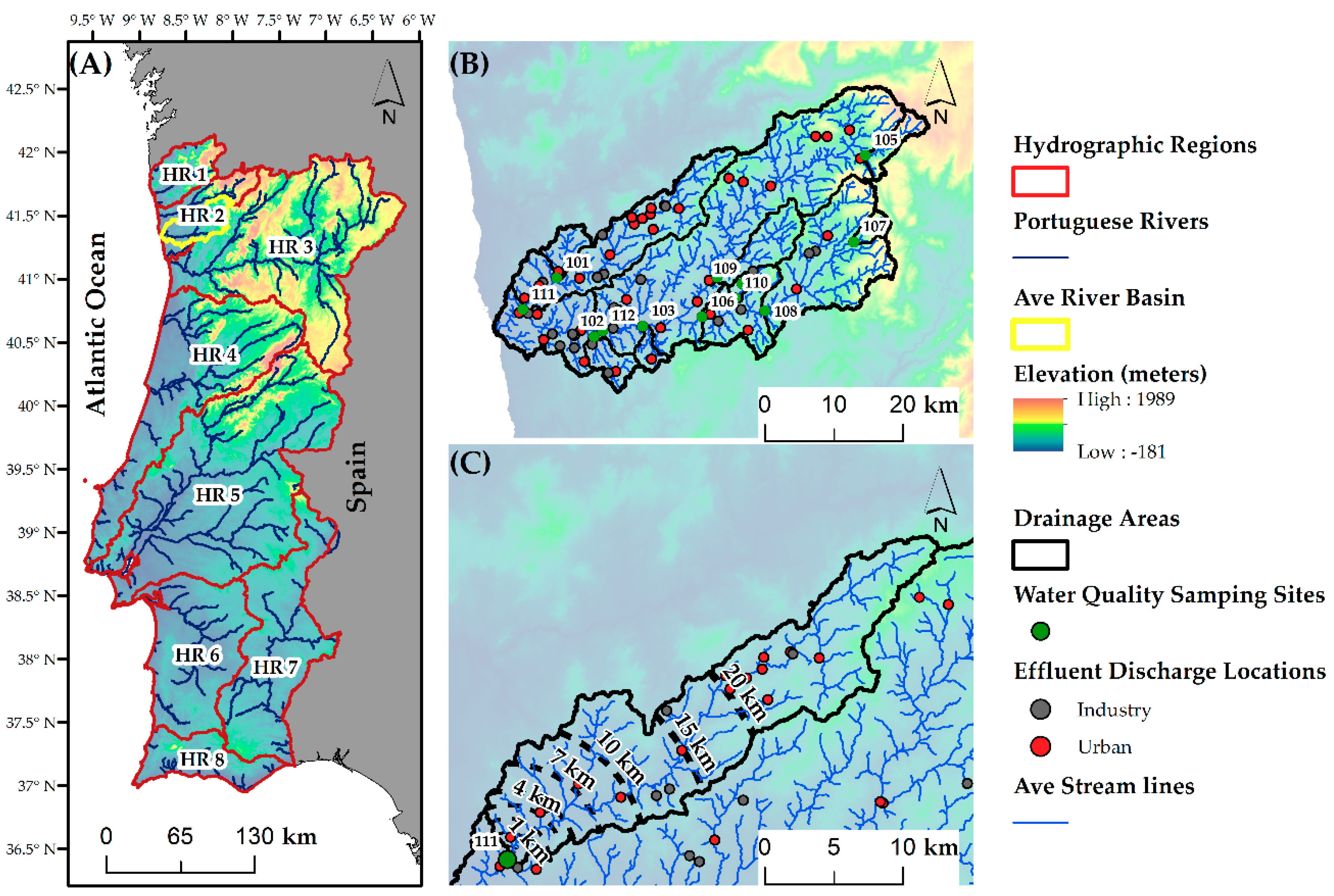
2.1. Study Area
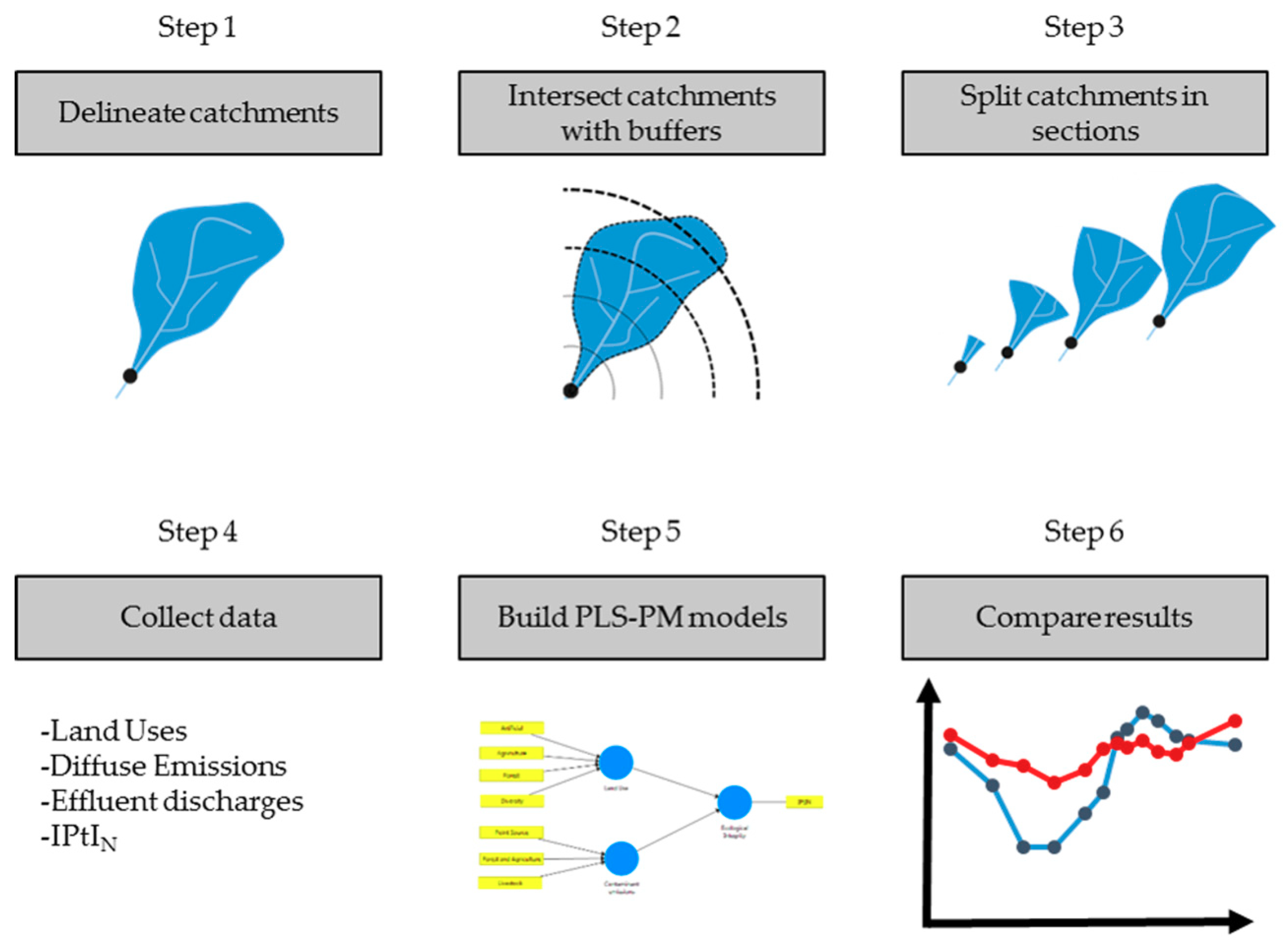
2.2. Workflow
2.3. Dataset
3. Results
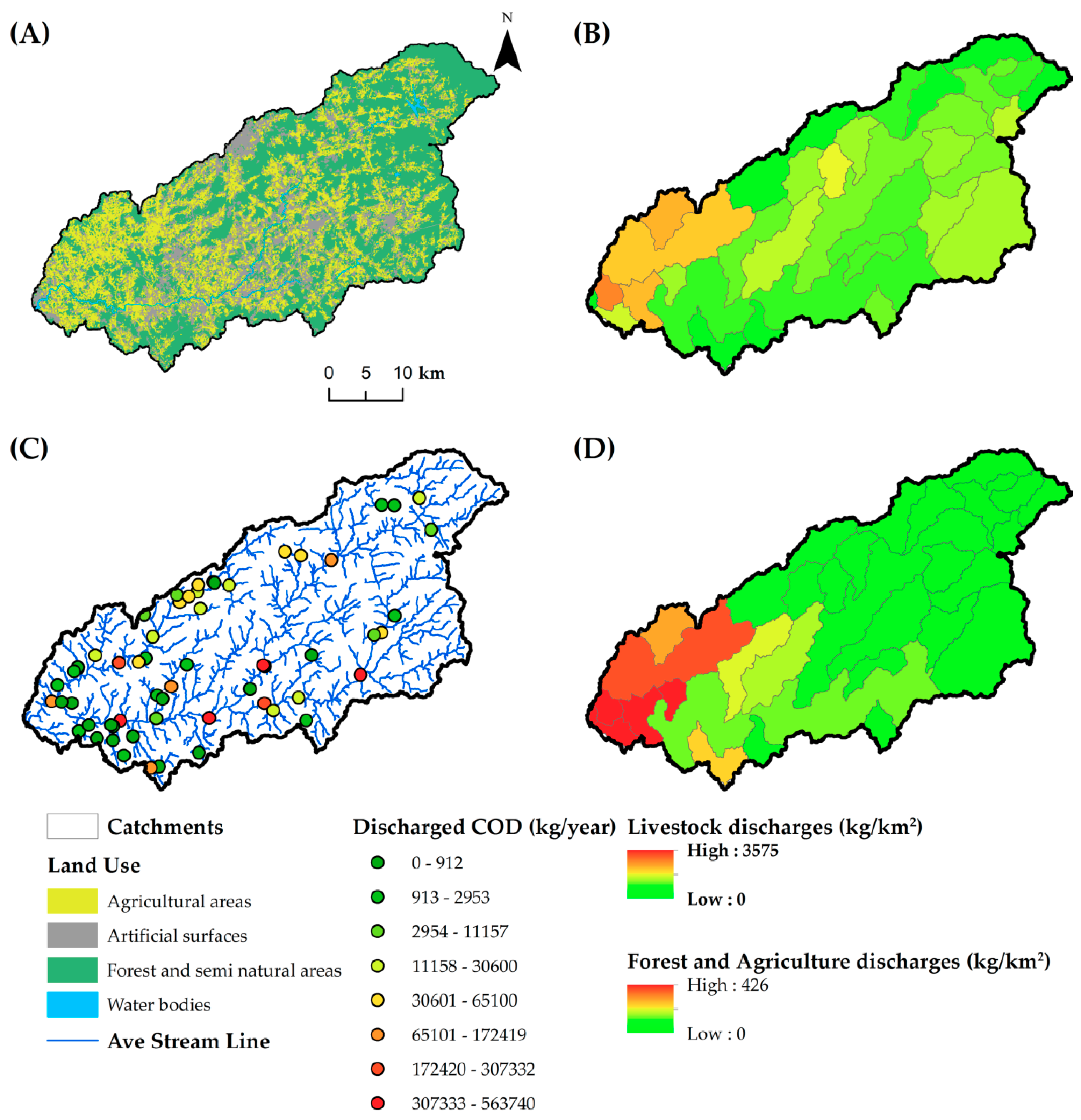
3.1. Spatial Data
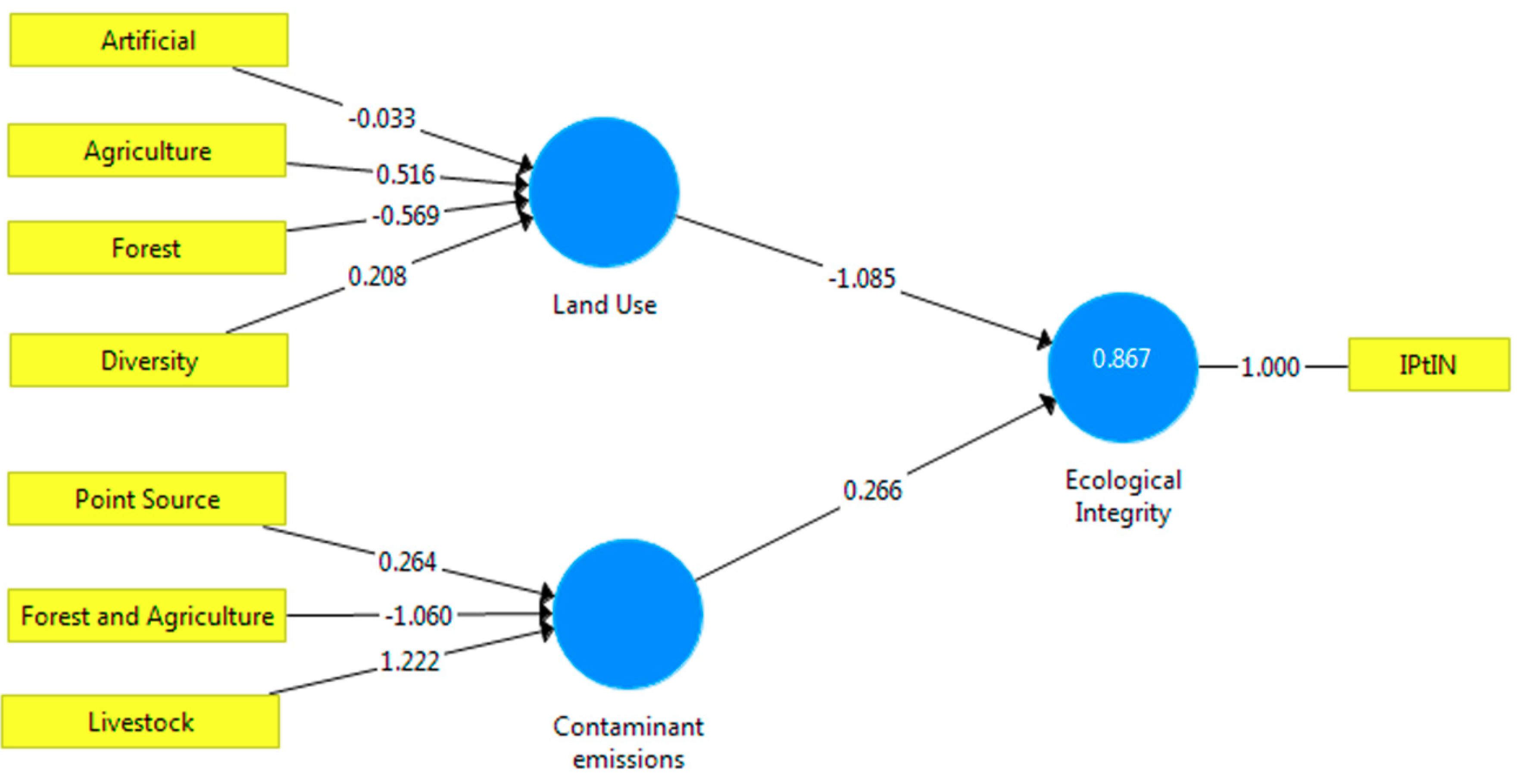
3.2. Interpretation of a PLS-PM Example Model
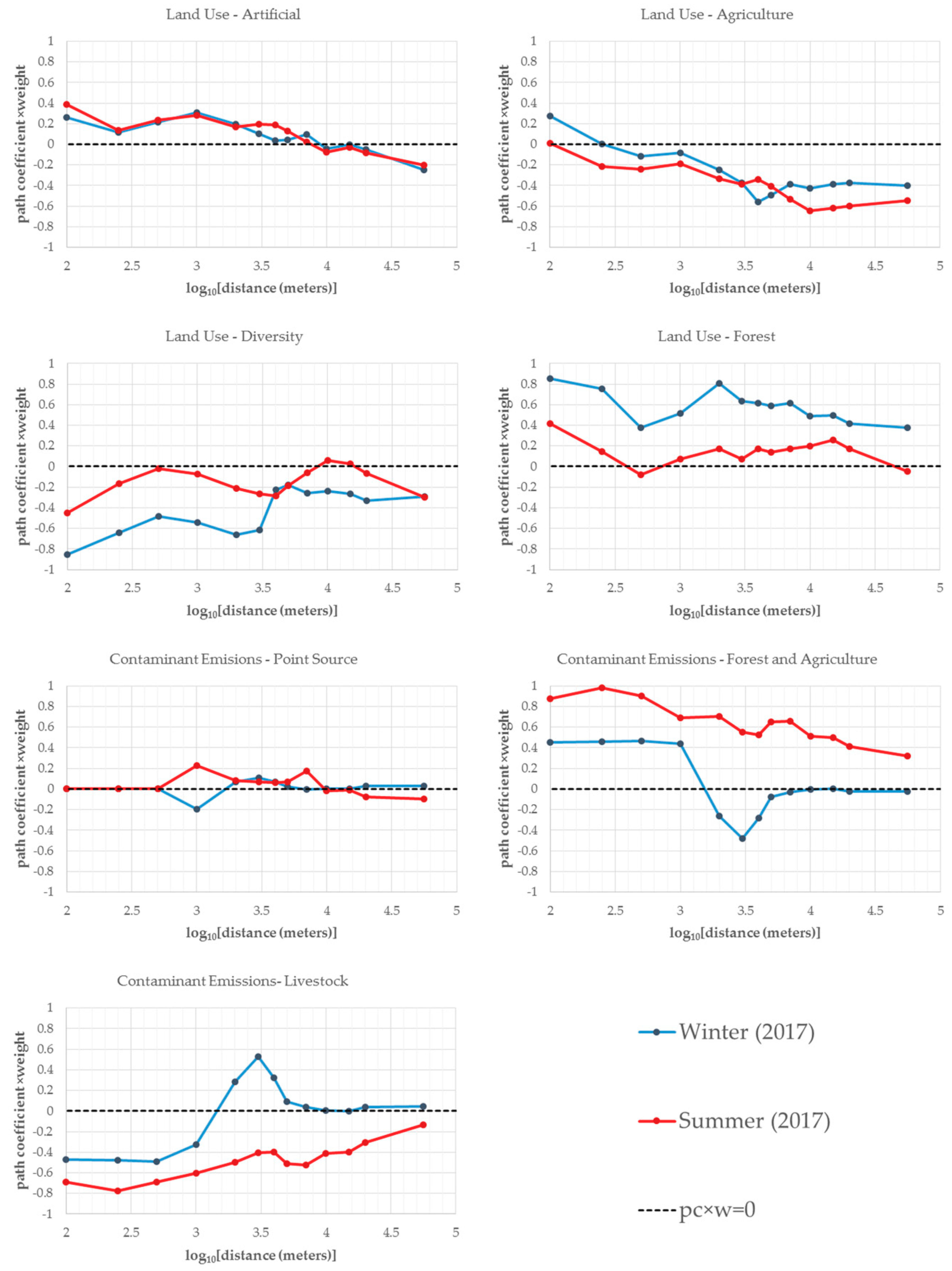
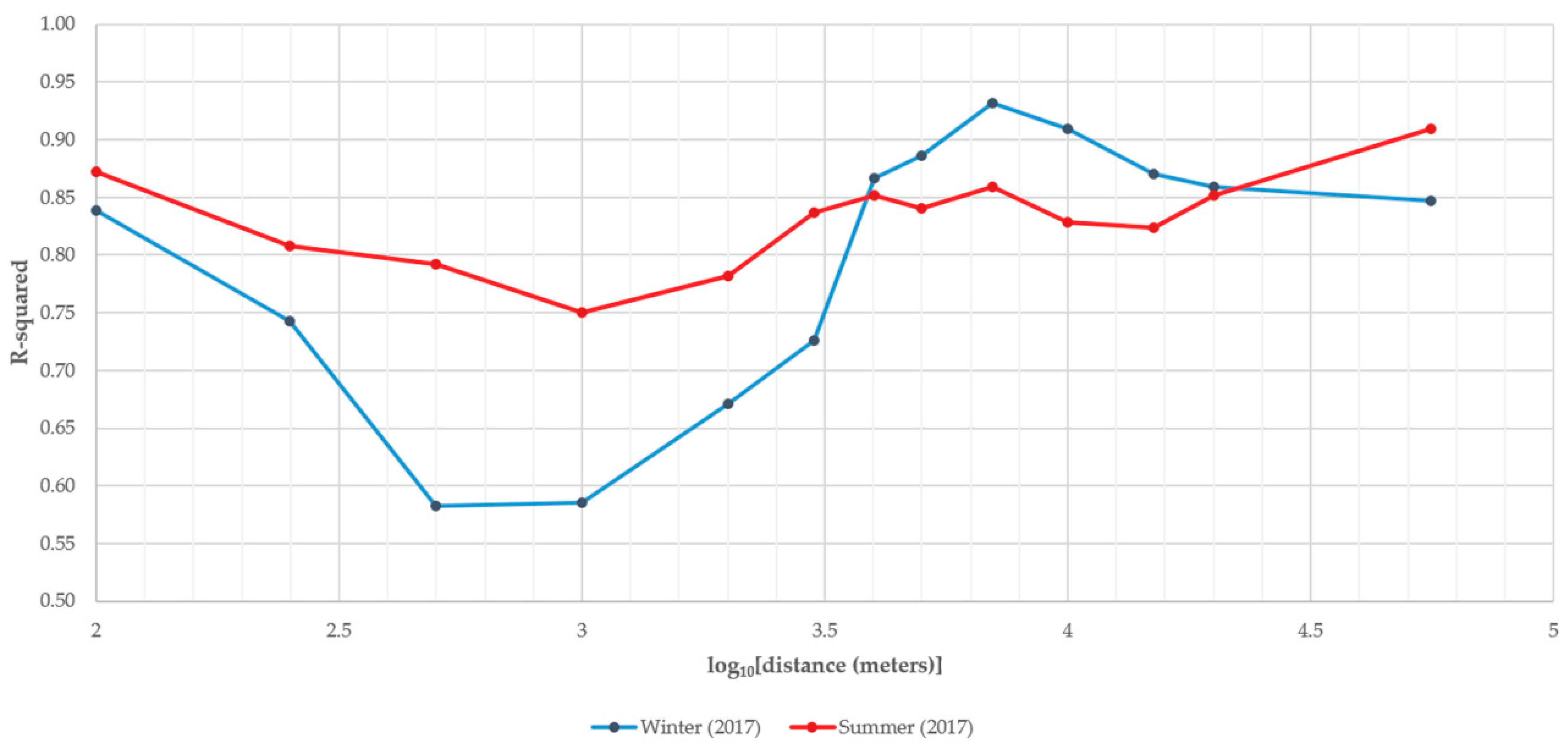
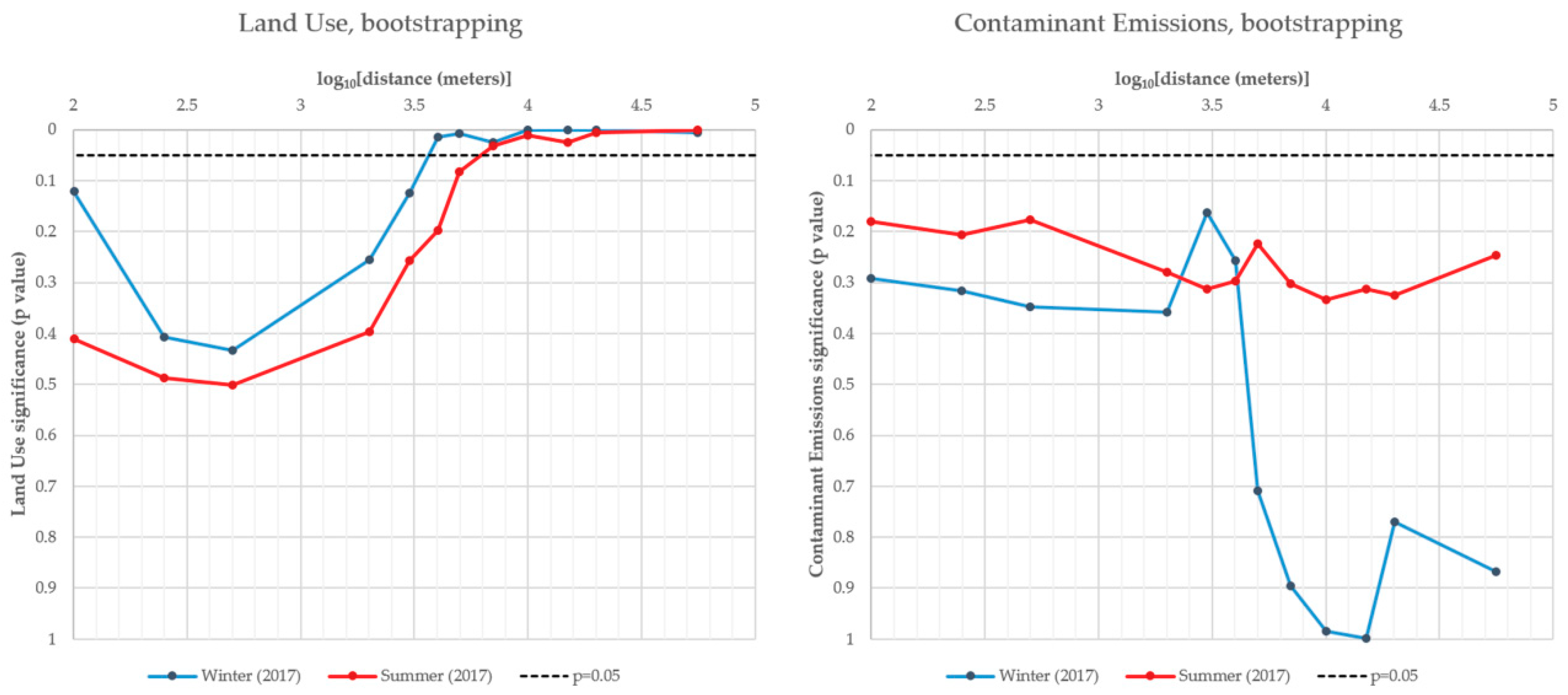
3.3. Results of All PLS-PM Models
4. Discussion
5. Conclusions
Supplementary Materials
Author Contributions
Funding
Conflicts of Interest
References
- Vorosmarty, C.J.; Green, P.; Salisbury, J.; Lammers, R.B. Global Water Resources: Vulnerability from Climate Change and Population Growth. Science 2000, 289, 284–288. [Google Scholar] [CrossRef] [PubMed] [Green Version]
- Delpla, I.; Jung, A.-V.; Baures, E.; Clement, M.; Thomas, O. Impacts of climate change on surface water quality in relation to drinking water production. Environ. Int. 2009, 35, 1225–1233. [Google Scholar] [CrossRef] [PubMed]
- Muga, H.E.; Mihelcic, J.R. Sustainability of wastewater treatment technologies. J. Environ. Manag. 2008, 88, 437–447. [Google Scholar] [CrossRef] [PubMed]
- Wright, J.; Gundry, S.; Conroy, R. Household drinking water in developing countries: A systematic review of microbiological contamination between source and point-of-use. Trop. Med. Int. Health 2004, 9, 106–117. [Google Scholar] [CrossRef] [PubMed]
- Hayet, C.; Saida, B.A.; Youssef, T.; Hédi, S. Study of biodegradability for municipal and industrial Tunisian wastewater by respirometric technique and batch reactor test. Sustain. Environ. Res. 2016, 26, 55–62. [Google Scholar] [CrossRef] [Green Version]
- Serrano-Grijalva, L.; Sánchez-Carrillo, S.; Angeler, D.G.; Sánchez-Andrés, R.; Álvarez-Cobelas, M. Effects of shrimp-farm effluents on the food web structure in subtropical coastal lagoons. J. Exp. Mar. Biol. Ecol. 2011, 402, 65–74. [Google Scholar] [CrossRef] [Green Version]
- Grizzetti, B.; Bouraoui, F.; De Marsily, G. Assessing nitrogen pressures on European surface water. Glob. Biogeochem. Cycles 2008, 22. [Google Scholar] [CrossRef]
- Sheoran, A.S.; Sheoran, V. Heavy metal removal mechanism of acid mine drainage in wetlands: A critical review. Miner. Eng. 2006, 19, 105–116. [Google Scholar] [CrossRef]
- Soares, H.M.V.; Boaventura, R.A.; Machado, A.A.S.; Esteves da Silva, J.C. Sediments as monitors of heavy metal contamination in the Ave river basin (Portugal): Multivariate analysis of data. Environ. Pollut. 1999, 105, 311–323. [Google Scholar] [CrossRef]
- Murphy, F.; Ewins, C.; Carbonnier, F.; Quinn, B. Wastewater Treatment Works (WwTW) as a Source of Microplastics in the Aquatic Environment. Environ. Sci. Technol. 2016, 50, 5800–5808. [Google Scholar] [CrossRef] [Green Version]
- Ayers, R.S.; Westcot, D.W. Water Quality for Agriculture; FAO United Nations: Rome, Italy, 1985. [Google Scholar]
- Nilsson, C.; Svedmark, M. Basic Principles and Ecological Consequences of Changing Water Regimes: Riparian Plant Communities. Environ. Manag. 2002, 30, 468–480. [Google Scholar] [CrossRef]
- Merritt, R.W.; Walker, E.D.; Small, P.L.C.; Wallace, J.R.; Johnson, P.D.R.; Benbow, M.E.; Boakye, D.A. Ecology and transmission of Buruli ulcer disease: A systematic review. PLoS Negl. Trop. Dis. 2010, 4, e911. [Google Scholar] [CrossRef] [PubMed]
- Santos, R.M.B.; Sanches Fernandes, L.F.; Varandas, S.G.P.; Pereira, M.G.; Sousa, R.; Teixeira, A.; Lopes-Lima, M.; Cortes, R.M.V.; Pacheco, F.A.L. Impacts of climate change and land-use scenarios on Margaritifera margaritifera, an environmental indicator and endangered species. Sci. Total Environ. 2015, 511, 477–488. [Google Scholar] [CrossRef] [PubMed]
- Townsend, S.A.; Douglas, M.M. The effect of a wildfire on stream water quality and catchment water yield in a tropical savanna excluded from fire for 10 years (Kakadu National Park, North Australia). Water Res. 2004, 38, 3051–3058. [Google Scholar] [CrossRef]
- Arkle, R.S.; Pilliod, D.S. Prescribed fires as ecological surrogates for wildfires: A stream and riparian perspective. For. Ecol. Manag. 2010, 259, 893–903. [Google Scholar] [CrossRef]
- Smith, H.G.; Sheridan, G.J.; Lane, P.N.J.; Nyman, P.; Haydon, S. Wildfire effects on water quality in forest catchments: A review with implications for water supply. J. Hydrol. 2011, 396, 170–192. [Google Scholar] [CrossRef]
- Santos, R.M.B.; Sanches Fernandes, L.F.; Pereira, M.G.; Cortes, R.M.V.; Pacheco, F.A.L. A framework model for investigating the export of phosphorus to surface waters in forested watersheds: Implications to management. Sci. Total Environ. 2015, 536, 295–305. [Google Scholar] [CrossRef]
- Júnior, R.; Galbiatti, J.A.; Pissarra, T.C.; Martins Filho, M. Diagnóstico do Conflito de Uso e Ocupação do Solo na Bacia do Rio Uberaba. Glob. Sci. Technol. 2013, 6, 40–52. [Google Scholar] [CrossRef]
- Pacheco, F.A.L.; Varandas, S.G.P.; Sanches Fernandes, L.F.; Valle Junior, R.F. Soil losses in rural watersheds with environmental land use conflicts. Sci. Total Environ. 2014, 485–486, 110–120. [Google Scholar] [CrossRef]
- Pacheco, F.A.L.; Sanches Fernandes, L.F. Environmental land use conflicts in catchments: A major cause of amplified nitrate in river water. Sci. Total Environ. 2016, 548–549, 173–188. [Google Scholar] [CrossRef]
- McGarigal, K. Landscape Pattern Metrics. In Wiley StatsRef: Statistics Reference Online; John Wiley & Sons Ltd.: Hoboken, NJ, USA, 2014. [Google Scholar]
- Uuemaa, E.; Roosaare, J.; Mander, Ü. Scale dependence of landscape metrics and their indicatory value for nutrient and organic matter losses from catchments. Ecol. Indic. 2005, 5, 350–369. [Google Scholar] [CrossRef]
- Lee, S.-W.; Hwang, S.-J.; Lee, S.-B.; Hwang, H.-S.; Sung, H.-C. Landscape ecological approach to the relationships of land use patterns in watersheds to water quality characteristics. Landsc. Urban Plan. 2009, 92, 80–89. [Google Scholar] [CrossRef]
- Łowicki, D. Prediction of flowing water pollution on the basis of landscape metrics as a tool supporting delimitation of Nitrate Vulnerable Zones. Ecol. Indic. 2012, 23, 27–33. [Google Scholar] [CrossRef]
- Wu, M.Y.; Xue, L.; Jin, W.B.; Xiong, Q.X.; Ai, T.C.; Li, B.L. Modelling the Linkage Between Landscape Metrics and Water Quality Indices of Hydrological Units in Sihu Basin, Hubei Province, China: An Allometric Model. Procedia Environ. Sci. 2012, 13, 2131–2145. [Google Scholar] [CrossRef] [Green Version]
- Wu, J.; Shen, W.; Sun, W.; Tueller, P.T. Empirical patterns of the effects of changing scale on landscape metrics. Landsc. Ecol. 2002, 17, 761–782. [Google Scholar] [CrossRef]
- Ding, J.; Jiang, Y.; Liu, Q.; Hou, Z.; Liao, J.; Fu, L.; Peng, Q. Influences of the land use pattern on water quality in low-order streams of the Dongjiang River basin, China: A multi-scale analysis. Sci. Total Environ. 2016, 551–552, 205–216. [Google Scholar] [CrossRef] [PubMed]
- Morley, S.A.; Karr, J.R. Assessing and restoring the health of urban streams in the Puget Sound Basin. Conserv. Biol. 2002, 16, 1498–1509. [Google Scholar] [CrossRef]
- Allan, J.D.; Erickson, D.L.; Fay, J. The influence of catchment land use on stream integrity across multiple spatial scales. Freshw. Biol. 1997, 37, 149–161. [Google Scholar] [CrossRef] [Green Version]
- Roth, N.E.; Allan, J.D.; Erickson, D.L. Landscape influences on stream biotic integrity assessed at multiple spatial scales. Landsc. Ecol. 1996, 11, 141–156. [Google Scholar] [CrossRef]
- Potter, K.M.; Cubbage, F.W.; Schaberg, R.H. Multiple-scale landscape predictors of benthic macroinvertebrate community structure in North Carolina. Landsc. Urban Plan. 2005, 71, 77–90. [Google Scholar] [CrossRef]
- Hunsaker, C.T.; Levine, D.A. Hierarchical Approaches to the Study of Water Quality in Rivers. Bioscience 1995, 45, 193–203. [Google Scholar] [CrossRef]
- Zhang, J.; Li, S.; Dong, R.; Jiang, C.; Ni, M. Influences of land use metrics at multi-spatial scales on seasonal water quality: A case study of river systems in the Three Gorges Reservoir Area, China. J. Clean. Prod. 2019, 206, 76–85. [Google Scholar] [CrossRef]
- Johnson, L.B.; Richards, C.; Host, G.E.; Arthur, J.W. Landscape influences on water chemistry in Midwestern stream ecosystems. Freshw. Biol. 1997, 37, 193–208. [Google Scholar] [CrossRef]
- Dodds, W.K.; Oakes, R.M. Headwater influences on downstream water quality. Environ. Manag. 2008, 41, 367–377. [Google Scholar] [CrossRef] [PubMed]
- Tran, C.P.; Bode, R.W.; Smith, A.J.; Kleppel, G.S. Land-use proximity as a basis for assessing stream water quality in New York State (USA). Ecol. Indic. 2010, 10, 727–733. [Google Scholar] [CrossRef]
- Schiff, R.; Benoit, G. Effects of impervious cover at multiple spatial scales on coastal watershed streams. J. Am. Water Resour. Assoc. 2007, 43, 712–730. [Google Scholar] [CrossRef]
- Yu, S.; Xu, Z.; Wu, W.; Zuo, D. Effect of land use types on stream water quality under seasonal variation and topographic characteristics in the Wei River basin, China. Ecol. Indic. 2016, 60, 202–212. [Google Scholar] [CrossRef]
- Thakur, A.K. Model: Mechanistic vs Empirical. In New Trends in Pharmacokinetics; Springer: Boston, MA, USA, 1991; pp. 41–51. [Google Scholar]
- Loucks, D.P.; van Beek, E. Water Quality Modelling and Prediction. In Water Resources Systems Planning and Management; UNESKO: Paris, France, 2005. [Google Scholar]
- Astrachan, C.B.; Patel, V.K.; Wanzenried, G. A comparative study of CB-SEM and PLS-SEM for theory development in family firm research. J. Fam. Bus. Strategy 2014, 5, 116–128. [Google Scholar] [CrossRef]
- Gorai, A.K.; Tuluri, F.; Tchounwou, P.B. Development of PLS–path model for understanding the role of precursors on ground level ozone concentration in Gulfport, Mississippi, USA. Atmos. Pollut. Res. 2015, 6, 389–397. [Google Scholar] [CrossRef]
- Chenini, I.; Khmiri, S. Evaluation of ground water quality using multiple linear regression and structural equation modeling. Int. J. Environ. Sci. Technol. 2009, 6, 509–519. [Google Scholar] [CrossRef] [Green Version]
- Levêque, J.G.; Burns, R.C. A Structural Equation Modeling approach to water quality perceptions. J. Environ. Manag. 2017, 197, 440–447. [Google Scholar] [CrossRef] [PubMed] [Green Version]
- Nugroho, A.R.; Masduqi, A. Structural equation modelling as instrument for water pollution factor analysis. In Proceedings of the 4th International Conference Advances in Applied Science and Environmental Technology—ASET 2016, Bangkok, Thailand, 7–8 May 2016. [Google Scholar]
- Martins, L.; Pereira, A.; Oliveira, A.; Fernandes, A.; Sanches Fernandes, L.F.; Pacheco, F.A.L. An assessment of groundwater contamination risk with radon based on clustering and structural models. Water 2019, 11, 1107. [Google Scholar] [CrossRef]
- Salgado Terêncio, D.P.; Sanches Fernandes, L.F.; Vitor Cortes, R.M.; Moura, J.P.; Leal Pacheco, F.A. Can Land Cover Changes Mitigate Large Floods? A Reflection Based on Partial Least Squares-Path Modeling. Water 2019, 11, 684. [Google Scholar] [CrossRef]
- Garcês, A.; Pires, I.; Pacheco, F.A.L.; Sanches Fernandes, L.F.; Soeiro, V.; Lóio, S.; Prada, J.; Cortes, R.; Queiroga, F.L. Preservation of wild bird species in northern Portugal—Effects of anthropogenic pressures in wild bird populations (2008–2017). Sci. Total Environ. 2019, 650, 2996–3006. [Google Scholar] [CrossRef] [PubMed]
- Ferreira, A.R.L.; Sanches Fernandes, L.F.; Cortes, R.M.V.; Pacheco, F.A.L. Assessing anthropogenic impacts on riverine ecosystems using nested partial least squares regression. Sci. Total Environ. 2017, 583, 466–477. [Google Scholar] [CrossRef] [PubMed]
- Sanches Fernandes, L.F.; Fernandes, A.C.P.; Ferreira, A.R.L.; Cortes, R.M.V.; Pacheco, F.A.L. A partial least squares—Path modeling analysis for the understanding of biodiversity loss in rural and urban watersheds in Portugal. Sci. Total Environ. 2018, 626, 1069–1085. [Google Scholar] [CrossRef] [PubMed]
- Fernandes, A.C.P.; Sanches Fernandes, L.F.; Moura, J.P.; Cortes, R.M.V.; Pacheco, F.A.L. A structural equation model to predict macroinvertebrate-based ecological status in catchments influenced by anthropogenic pressures. Sci. Total Environ. 2019, 681, 242–257. [Google Scholar] [CrossRef]
- APA—ARH-Norte. Plano de Gestão da Região Hidrográfica do Cávado, Ave e Leça (RH2). Relatório Base 1o Ciclo Parte 1—Enquadramento e Aspectos Gerais; Agência Portuguesa do Ambiente: Porto, Portugal, 2012. [Google Scholar]
- Gonçalves, E.P.R.; Boaventura, R.A.R.; Mouvet, C. Sediments and aquatic mosses as pollution indicators for heavy metals in the Ave river basin (Portugal). Sci. Total Environ. 1992, 114, 7–24. [Google Scholar] [CrossRef]
- Alves, C.; Boaventura, R.; Soares, H. Evaluation of Heavy Metals Pollution Loadings in the Sediments of the Ave River Basin (Portugal). Soil Sediment. Contam. 2009, 18, 603–618. [Google Scholar] [CrossRef]
- Peixoto, F.P.; Carrola, J.; Coimbra, A.M.; Teixeira, P.; Coelho, L.; Conceição, I.; Oliveira, M.M.; Fontaínhas-Fernandes, A.; Fernandes, C. Oxidative stress responses and histological hepatic alterations in barbel, Barbus bocagei, from Vizela River, Portugal. Rev. Int. Contam. Ambient. 2013, 29, 29–38. [Google Scholar]
- Pascoal, C.; Pinho, M.; Cássio, F.; Gomes, P. Assessing structural and functional ecosystem condition using leaf breakdown: Studies on a polluted river. Freshw. Biol. 2003, 48, 2033–2044. [Google Scholar] [CrossRef]
- Pascoal, C.; Cássio, F.; Marvanová, L. Anthropogenic stress may affect aquatic hyphomycete diversity more than leaf decomposition in a low-order stream. Arch. Hydrobiol. 2005, 162, 481–496. [Google Scholar] [CrossRef]
- Dunck, B.; Lima-Fernandes, E.; Cássio, F.; Cunha, A.; Rodrigues, L.; Pascoal, C. Responses of primary production, leaf litter decomposition and associated communities to stream eutrophication. Environ. Pollut. 2015, 202, 32–40. [Google Scholar] [CrossRef] [PubMed]
- Pinto, D.; Fernandes, A.; Fernandes, R.; Mendes, I.; Pereira, S.; Vinha, A.; Herdeiro, T.; Santos, E.; Machado, M. Determination of heavy metals and other indicators in waters, soils and medicinal plants from Ave valley, in Portugal, and its correlation to urban and industrial pollution. Sci. Microb. Pathog. Commun. Curr. Res. Technol. Adv. 2011, 303–309. [Google Scholar]
- Ribeiro, C.M.R.; Maia, A.S.; Ribeiro, A.R.; Couto, C.; Almeida, A.A.; Santos, M.; Tiritan, M.E. Anthropogenic pressure in a Portuguese river: Endocrine-disrupting compounds, trace elements and nutrients. J. Environ. Sci. Health Part. A 2016, 51, 1043–1052. [Google Scholar] [CrossRef]
- Environmental Systems Resource Institute. ArcMap 10.2.; ESRI: Redlands, CA, USA, 2014. [Google Scholar]
- Maidment, D.R. Arc Hydro: GIS for Water Resources; ESRI Inc.: Redlands, CA, USA, 2002. [Google Scholar]
- Santos, R.M.B.; Sanches Fernandes, L.F.; Cortes, R.M.V.; Varandas, S.G.P.; Jesus, J.J.B.; Pacheco, F.A.L. Integrative assessment of river damming impacts on aquatic fauna in a Portuguese reservoir. Sci. Total Environ. 2017, 601, 1108–1118. [Google Scholar] [CrossRef]
- Fonseca, A.R.; Sanches Fernandes, L.F.; Fontainhas-Fernandes, A.; Monteiro, S.M.; Pacheco, F.A.L. The impact of freshwater metal concentrations on the severity of histopathological changes in fish gills: A statistical perspective. Sci. Total Environ. 2017, 599, 217–226. [Google Scholar] [CrossRef] [PubMed]
- Pacheco, F.A.L. Regional groundwater flow in hard rocks. Sci. Total Environ. 2015, 506, 182–195. [Google Scholar] [CrossRef] [PubMed]
- Pacheco, F.A.L.; Sousa Oliveira, A.; Van Der Weijden, A.J.; Van Der Weijden, C.H. Weathering, biomass production and groundwater chemistry in an area of dominant anthropogenic influence, the Chaves-Vila Pouca de Aguiar region, north of Portugal. Water Air Soil Pollut. 1999, 115, 481–512. [Google Scholar] [CrossRef]
- Pacheco, F.A.L.; Landim, P.M.B. Two-Way Regionalized Classification of Multivariate Datasets and its Application to the Assessment of Hydrodynamic Dispersion. Math. Geol. 2005, 37, 393–417. [Google Scholar] [CrossRef] [Green Version]
- Pacheco, F.A.L.; Landim, P.M.B.; Szocs, T. Anthropogenic impacts on mineral weathering: A statistical perspective. Appl. Geochem. 2013, 36, 34–48. [Google Scholar] [CrossRef]
- Valle Junior, R.F.; Varandas, S.G.P.; Sanches Fernandes, L.F.; Pacheco, F.A.L. Multi Criteria Analysis for the monitoring of aquifer vulnerability: A scientific tool in environmental policy. Environ. Sci. Policy 2015, 48, 250–264. [Google Scholar] [CrossRef] [Green Version]
- Valera, C.A.; Pissarra, T.C.T.; Martins Filho, M.V.; Valle Junior, R.F.; Sanches Fernandes, L.F.; Pacheco, F.A.L. A legal framework with scientific basis for applying the ‘polluter pays principle’ to soil conservation in rural watersheds in Brazil. Land Use Policy 2017, 66, 61–71. [Google Scholar] [CrossRef]
- Environmental Systems Resource Institute. ArcHydro Tools for ArcGIS 10—Tutorial; ESRI: Redlands, CA, USA, 2012. [Google Scholar]
- Ring, C.M.; Wende, S.; Will, A. Smart PLS. Hamburg, Germany. 2005. Available online: http//www.smartpls.de (accessed on 1 May 2019).
- Hair, J.F., Jr.; Sarstedt, M.; Hopkins, L.; Kuppelwieser, V.G. Partial least squares structural equation modeling (PLS-SEM). Eur. Bus. Rev. 2014, 26, 106–121. [Google Scholar] [CrossRef]
- Schindler, U.; Klinner, K.; Nestler, W. Microsoft® Excel—Grundlagen der Makroprogrammierung; Springer: Berlin/Heidelberg, Germany, 2013. [Google Scholar]
- Adamczyk, J.; Tiede, D. ZonalMetrics—A Python toolbox for zonal landscape structure analysis. Comput. Geosci. 2017, 99, 91–99. [Google Scholar] [CrossRef]
- APA Critérios de Classificação do Estado das Massas de Água—Rios e Albufeiras. Available online: https://www.apambiente.pt/dqa/criterios-classificacao.html (accessed on 22 June 2019).
- UKTAG (UKTechnical Advisory Group on the WaterFramework Directive). Technical Report on Groundwater Hazardous Substances. 2016. Available online: https://www.wfduk.org (accessed on 22 June 2019).
- European Commission. Monitoring under the Water Framework Directive. In Common Implementation Strategy for the Water Framework Directive (2000/60/EC); European Commission: Brussels, Belgium, 2003. [Google Scholar]
- Pielou, E.C. The measurement of diversity in different types of biological collections. J. Theor. Biol. 1966, 13, 131–144. [Google Scholar] [CrossRef]
- Jost, L. The Relation between Evenness and Diversity. Diversity 2010, 2, 207–232. [Google Scholar] [CrossRef]
- Devís-Devís, J.; Villamón-Herrera, M. A scientific field searching visibility. International Workshop on Physical Activity and Sport Sciences Quality Journals. Proc. Prof. Inf. 2008, 17, 242–246. [Google Scholar]
- Ketchen, D.J. A Primer on Partial Least Squares Structural Equation Modeling. Long Range Plan. 2013, 46, 184–185. [Google Scholar] [CrossRef]
- Neary, D.G.; Ice, G.G.; Jackson, C.R. Linkages between forest soils and water quality and quantity. For. Ecol. Manag. 2009, 258, 2269–2281. [Google Scholar] [CrossRef]
- Snyder, C.D.; Young, J.A.; Villella, R.; Lemarié, D.P. Influences of upland and riparian land use patterns on stream biotic integrity. Landsc. Ecol. 2003, 18, 647–664. [Google Scholar] [CrossRef]
- Sliva, L.; Dudley Williams, D. Buffer Zone versus Whole Catchment Approaches to Studying Land Use Impact on River Water Quality. Water Res. 2001, 35, 3462–3472. [Google Scholar] [CrossRef]
- Bu, H.; Meng, W.; Zhang, Y.; Wan, J. Relationships between land use patterns and water quality in the Taizi River basin, China. Ecol. Indic. 2014, 41, 187–197. [Google Scholar] [CrossRef]
- Grizzetti, B.; Bouraoui, F.; de Marsily, G.; Bidoglio, G. A statistical method for source apportionment of riverine nitrogen loads. J. Hydrol. 2005, 304, 302–315. [Google Scholar] [CrossRef]
- Bowes, M.J.; Smith, J.T.; Jarvie, H.P.; Neal, C.; Barden, R. Changes in point and diffuse source phosphorus inputs to the River Frome (Dorset, UK) from 1966 to 2006. Sci. Total Environ. 2009, 407, 1954–1966. [Google Scholar] [CrossRef]
- Heathwaite, A.L.; Dils, R.M.; Liu, S.; Carvalho, L.; Brazier, R.E.; Pope, L.; Hughes, M.; Phillips, G.; May, L. A tiered risk-based approach for predicting diffuse and point source phosphorus losses in agricultural areas. Sci. Total Environ. 2005, 344, 225–239. [Google Scholar] [CrossRef] [PubMed]
- Spieles, D.J.; Mitsch, W.J. The effects of season and hydrologic and chemical loading on nitrate retention in constructed wetlands: A comparison of low- and high-nutrient riverine systems. Ecol. Eng. 1999, 14, 77–91. [Google Scholar] [CrossRef]
- Jones, J.P.; Sudicky, E.A.; Brookfield, A.E.; Park, Y.-J. An assessment of the tracer-based approach to quantifying groundwater contributions to streamflow. Water Resour. Res. 2006, 42. [Google Scholar] [CrossRef] [Green Version]
- Coltman, T.; Devinney, T.M.; Midgley, D.F.; Venaik, S. Formative versus reflective measurement models: Two applications of formative measurement. J. Bus. Res. 2008, 61, 1250–1262. [Google Scholar] [CrossRef] [Green Version]
- McGarigal, K.; Marks, B.J. FRAGSTATS: Spatial Pattern Analysis Program for Quantifying Landscape Structure; U.S. Department Agriculture Forest Service/Pacific Northwest Research Station: Washington, DC, USA, 1995.


| Data | Description | Source |
|---|---|---|
| Elevation model | Elevation model raster file, with a pixel size of 25 per 25 m. | http://www.eea.europa.eu |
| Effluent discharge points | Flow of discharged biological and chemical oxygen demands, nitrogen and phosphorous from urban effluents in surface water and underground water. | http://www.apambiente.pt |
| Diffuse discharge values | Nitrogen and phosphorous yields sourced from agriculture, forest, and livestock production areas. | http://www.apambiente.pt |
| Land use | Land uses map of Portuguese territory in 2015. | http://www.dgterritorio.pt |
| Macroinvertebrate index (IPtIN) | Biodiversity of benthic macroinvertebrates | measured in field |
| Site | Winter 2017 | Summer 2017 | ||
|---|---|---|---|---|
| Value | Classification | Value | Classification | |
| 101 | 0.415 | Poor | 0.979 | Excellent |
| 102 | 0.632 | Moderate | 0.398 | Poor |
| 103 | 0.389 | Poor | 0.364 | Poor |
| 104 | 0.113 | Very Poor | 0.498 | Moderate |
| 105 | 1.048 | Excellent | 1.017 | Excellent |
| 106 | 0.307 | Poor | 0.512 | Moderate |
| 107 | 1.050 | Excellent | 0.936 | Excellent |
| 108 | 0.493 | Moderate | 0.582 | Moderate |
| 109 | 0.138 | Very Poor | 0.346 | Poor |
| 110 | 0.522 | Moderate | 0.308 | Poor |
| 111 | 0.432 | Moderate | 0.397 | Poor |
| 112 | 0.219 | Poor | 0.275 | Poor |
© 2019 by the authors. Licensee MDPI, Basel, Switzerland. This article is an open access article distributed under the terms and conditions of the Creative Commons Attribution (CC BY) license (http://creativecommons.org/licenses/by/4.0/).
Share and Cite
Fernandes, A.C.P.; Sanches Fernandes, L.F.; Cortes, R.M.V.; Leal Pacheco, F.A. The Role of Landscape Configuration, Season, and Distance from Contaminant Sources on the Degradation of Stream Water Quality in Urban Catchments. Water 2019, 11, 2025. https://doi.org/10.3390/w11102025
Fernandes ACP, Sanches Fernandes LF, Cortes RMV, Leal Pacheco FA. The Role of Landscape Configuration, Season, and Distance from Contaminant Sources on the Degradation of Stream Water Quality in Urban Catchments. Water. 2019; 11(10):2025. https://doi.org/10.3390/w11102025
Chicago/Turabian StyleFernandes, António Carlos Pinheiro, Luís Filipe Sanches Fernandes, Rui Manuel Vitor Cortes, and Fernando António Leal Pacheco. 2019. "The Role of Landscape Configuration, Season, and Distance from Contaminant Sources on the Degradation of Stream Water Quality in Urban Catchments" Water 11, no. 10: 2025. https://doi.org/10.3390/w11102025