Article

A Hybrid Computational Intelligence Approach to Groundwater Spring Potential Mapping

1
Geographic Information Science Research Group, Ton Duc Thang University, Ho Chi Minh City, Vietnam
2
Faculty of Environment and Labour Safety, Ton Duc Thang University, Ho Chi Minh City, Vietnam
3
Department of Rangeland and Watershed Management, Faculty of Natural Resources, University of Kurdistan, Sanandaj 66177-15175, Iran
4
Department of Geomorphology, Faculty of Natural Resources, University of Kurdistan, Sanandaj 66177-15175, Iran
5
Center for Advanced Modeling and Geospatial System (CAMGIS), Faculty of Engineering and IT, University of Technology Sydney, CB11.06.106, Building 11, 81 Broadway, Sydney, NSW 2007, Australia
6
Department of Energy and Mineral Resources Engineering, Sejong University, Choongmu-gwan, 209 Neungdong-ro, Gwangjin-gu, Seoul 05006, Korea
7
Institute of Research and Development, Duy Tan University, Da Nang 550000, Vietnam
8
Department of Biological and Agricultural Engineering & Zachry Department of Civil Engineering, Texas A & M University, College Station, TX 77843-2117, USA
9
College of Geology and Environment, Xi’an University of Science and Technology, Xi’an 710054, China
10
School of Engineering, University of Guelph, Guelph, ON N1G 2W1, Canada
11
Faculty of Built Environment and Surveying, Universiti Teknologi Malaysia (UTM), 81310 Johor Bahru, Malaysia
12
Geoscience Platform Research Division, Korea Institute of Geoscience and Mineral Resources (KIGAM), 124, Gwahak-ro Yuseong-gu, Daejeon 34132, Korea
13
Department of Geophysical Exploration, Korea University of Science and Technology, 217 Gajeong-ro Yuseong-gu, Daejeon 34113, Korea
*
Authors to whom correspondence should be addressed.
Water 2019, 11(10), 2013; https://doi.org/10.3390/w11102013
Submission received: 20 July 2019 / Revised: 21 September 2019 / Accepted: 22 September 2019 / Published: 27 September 2019
(This article belongs to the Special Issue Characterizing Groundwater - Surface Water Interaction Using GIS)

Abstract

:
This study proposes a hybrid computational intelligence model that is a combination of alternating decision tree (ADTree) classifier and AdaBoost (AB) ensemble, namely “AB–ADTree”, for groundwater spring potential mapping (GSPM) at the Chilgazi watershed in the Kurdistan province, Iran. Although ADTree and its ensembles have been widely used for environmental and ecological modeling, they have rarely been applied to GSPM. To that end, a groundwater spring inventory map and thirteen conditioning factors tested by the chi-square attribute evaluation (CSAE) technique were used to generate training and testing datasets for constructing and validating the proposed model. The performance of the proposed model was evaluated using statistical-index-based measures, such as positive predictive value (PPV), negative predictive value (NPV), sensitivity, specificity accuracy, root mean square error (RMSE), and the area under the receiver operating characteristic (ROC) curve (AUROC). The proposed hybrid model was also compared with five state-of-the-art benchmark soft computing models, including single ADTree, support vector machine (SVM), stochastic gradient descent (SGD), logistic model tree (LMT), logistic regression (LR), and random forest (RF). Results indicate that the proposed hybrid model significantly improved the predictive capability of the ADTree-based classifier (AUROC = 0.789). In addition, it was found that the hybrid model, AB–ADTree, (AUROC = 0.815), had the highest goodness-of-fit and prediction accuracy, followed by the LMT (AUROC = 0.803), RF (AUC = 0.803), SGD, and SVM (AUROC = 0.790) models. Indeed, this model is a powerful and robust technique for mapping of groundwater spring potential in the study area. Therefore, the proposed model is a promising tool to help planners, decision makers, managers, and governments in the management and planning of groundwater resources.

1. Introduction

Groundwater serves as the source of water supply needed for different sectors, including agriculture, industry, animal husbandry, and communities in many countries around the world [1,2]. Groundwater is often the result of infiltration of rainwater, snowmelt water into soil and underlying rocks, and thereupon fills the pore space of soil and rocks [3,4]. Recently, based on the Bundesanstalt für Geowissenschaften und Rohstoffe [5] report, the consumption of groundwater has increased over the last few years, such that it amounts to 1000 km3, while the recharge of groundwater globally has reached 12,700 km3/year [5]. Furthermore, the level of pollution and wider distribution of groundwater is low, which, in turn, has attracted more human population throughout the world [6].
In Iran, most of the people living in rural and urban areas (70%) are dependent on groundwater as a safe water resource [7]. In recent years, due to climate change and intensive withdrawal of available groundwater resources, many regions of Iran have become dry and semi-dry, which has caused a serious lack of water throughout the country [1,2,8,9,10,11,12]. Since groundwater consumption in Iran has been increasing dramatically, development of proper methods to assess the aquifer productivity and groundwater potential areas are badly needed. These methods are essential for future systematic development, profitable management, and arresting the decline of groundwater resources [13]. Due to the requirement of fresh groundwater increases, plans for groundwater spring potential zones become an important task to successfully determine, manage, and protect groundwater programs. Therefore, groundwater spring potential mapping (GSPM) is important for protecting water quality and managing the use of groundwater [14]. Hence, GSPM is useful for proper groundwater protection and management [15].
In recent decades, remote sensing (RS) integrated with geographical information system (GIS) has been popularly applied for GSPM [16,17,18,19,20,21,22,23,24,25,26,27,28,29]. Many statistical models have been applied to GSPM, such as analytical hierarchy process (AHP) [12,30,31,32,33], frequency ratio (FR) [13,15], multi-criteria decision analysis (MCDA) [34,35,36], weight of evidence (WofE) [37,38,39], and evidential belief function (EBF) [40,41,42,43].
In recent years, machine learning algorithms (MLAs) have been proposed and suggested to solve many real world problems, including groundwater spring potential mapping, which are logistic regression (LR) [22,37,44], random forest [12,14,42], Naive Bayes [45], and decision tree (DT) [46,47,48]. However, they are also widely used in some fields of hydrology worldwide, including (i) surface water hydrology, such as rainfall and runoff forecasting [49,50], stream flow and sediment yield forecasting [51,52], evaporation and evapotranspiration forecasting [53,54,55], lake and reservoir water level prediction [56,57], flood susceptibility mapping and forecasting [58,59,60,61,62], and snow avalanche forecasting [63]; (ii) groundwater hydrology, such as groundwater level prediction [64], soil moisture estimation [65], and groundwater quality assessment [66].
More recently, machine learning ensemble models have been shown to be better than conventional methods in many fields, especially in natural hazards such as floods [58,59,62,67,68,69,70,71], wildfires [72], sinkholes [73], droughts [74], earthquakes [75,76], gully erosion [77,78], land/ground subsidence [79], and landslides [80,81,82,83,84,85,86,87,88,89,90,91,92,93,94,95,96,97,98,99,100,101,102,103,104,105,106,107,108]. However, exploration of these methods for GSPM has always been considered a big challenge. On the other hand, due to the flexibility and high prediction power of machine learning ensemble models, they are more applied in water studies, such as GSPM. Literature review shows that some methods have been used to identify areas with high potential of groundwater. In other words, modeling has not only continued, but it has progressed more rapidly in recent years in many fields. This illustrates that the subject of groundwater is of great importance and is being pursued to achieve high-precision maps to avoid costly traditional groundwater exploration methods and also to use groundwater aquifers in critical times, especially in drought periods. Achieving groundwater potential maps with high prediction accuracy by hybrid techniques seems to be a necessity these days. Therefore, the main objective of this study was to use a hybrid machine learning model for mapping areas with high potential of groundwater at Chilgazi watershed, northwest of Iran. In this study, the ADTree algorithm as a single/base algorithm and AdaBoost (AB) as a Mate classifier algorithm were selected for modeling groundwater. The AB algorithm is a powerful ensemble that combines sub-training datasets. Then, an ADTree was performed on each dataset, and finally, all these datasets were summed and output was achieved. This process enhanced the prediction power of ADTree and results were found more reasonable. The ensembles of ADTree algorithm are still rare in groundwater potential mapping.
Therefore, this study can be considered as a pioneering work in this area. The generated maps can be useful for decision makers, planners, managers, and government agencies for the sustainable management of ground water resources. The main objectives of this study were (i) applying an ensemble machine learning model, AB–ADTree, for groundwater spring potential mapping; (ii) selecting the most important conditioning factors for groundwater productivity; and (iii) comparing the performance of the applied model and also suggesting a promising model for groundwater exploitation instead of traditional methods, such as drilling, hydro-geological, geological, and geophysical. Additionally, we compared and validated the results obtained from the proposed model with six state-of-the-art soft computing benchmark models, including logistic regression (LR), logistic model tree (LMT), stochastic gradient descent (SGD), support vector machine (SVM), alternating decision tree (ADTree), and random forest (RF). Modeling process and susceptibility maps were done in Weka 3.6.9 and ArcGIS 10.3, respectively.

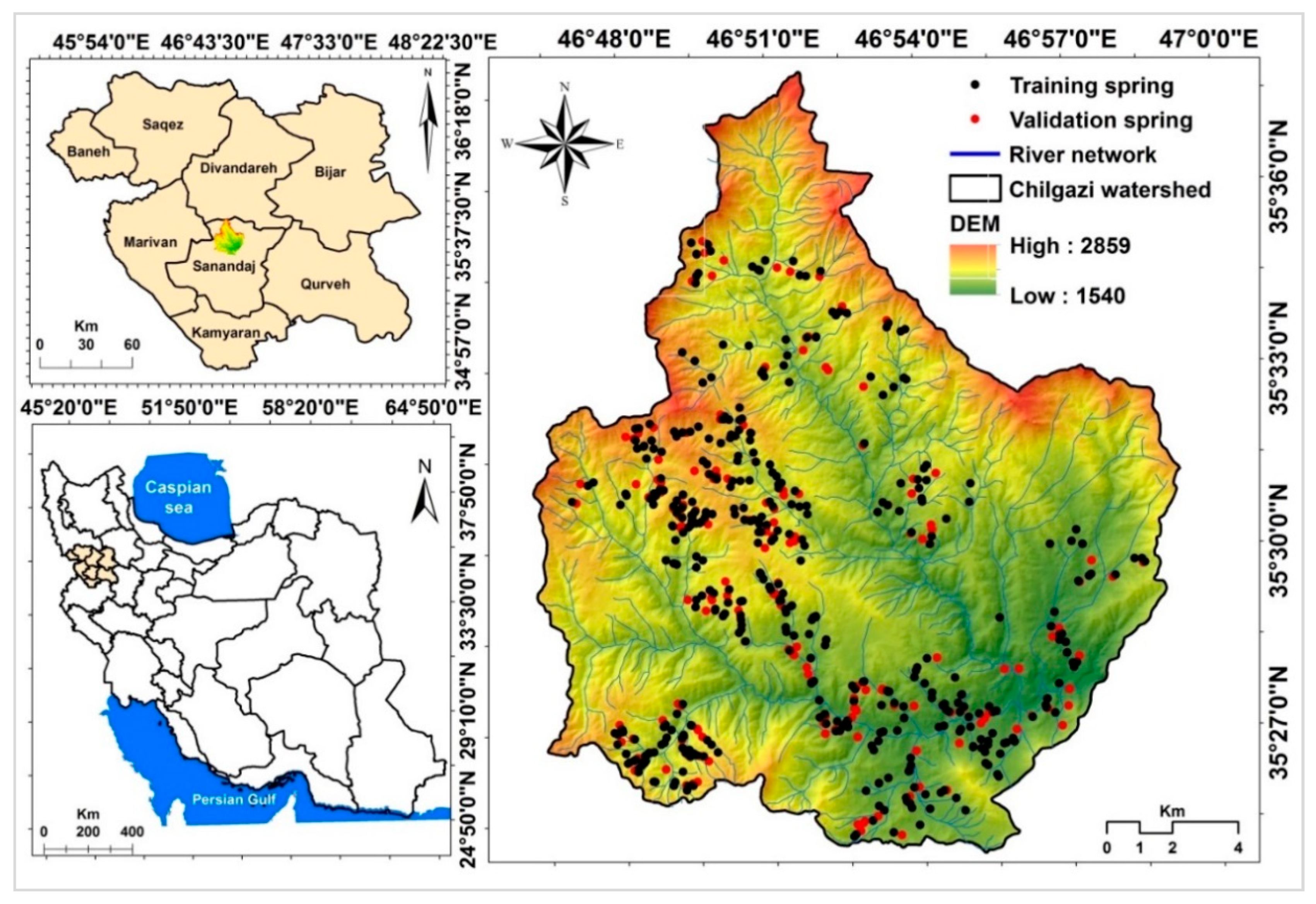
2. Research Area and Groundwater Spring Geodatabase

Description of Research Area
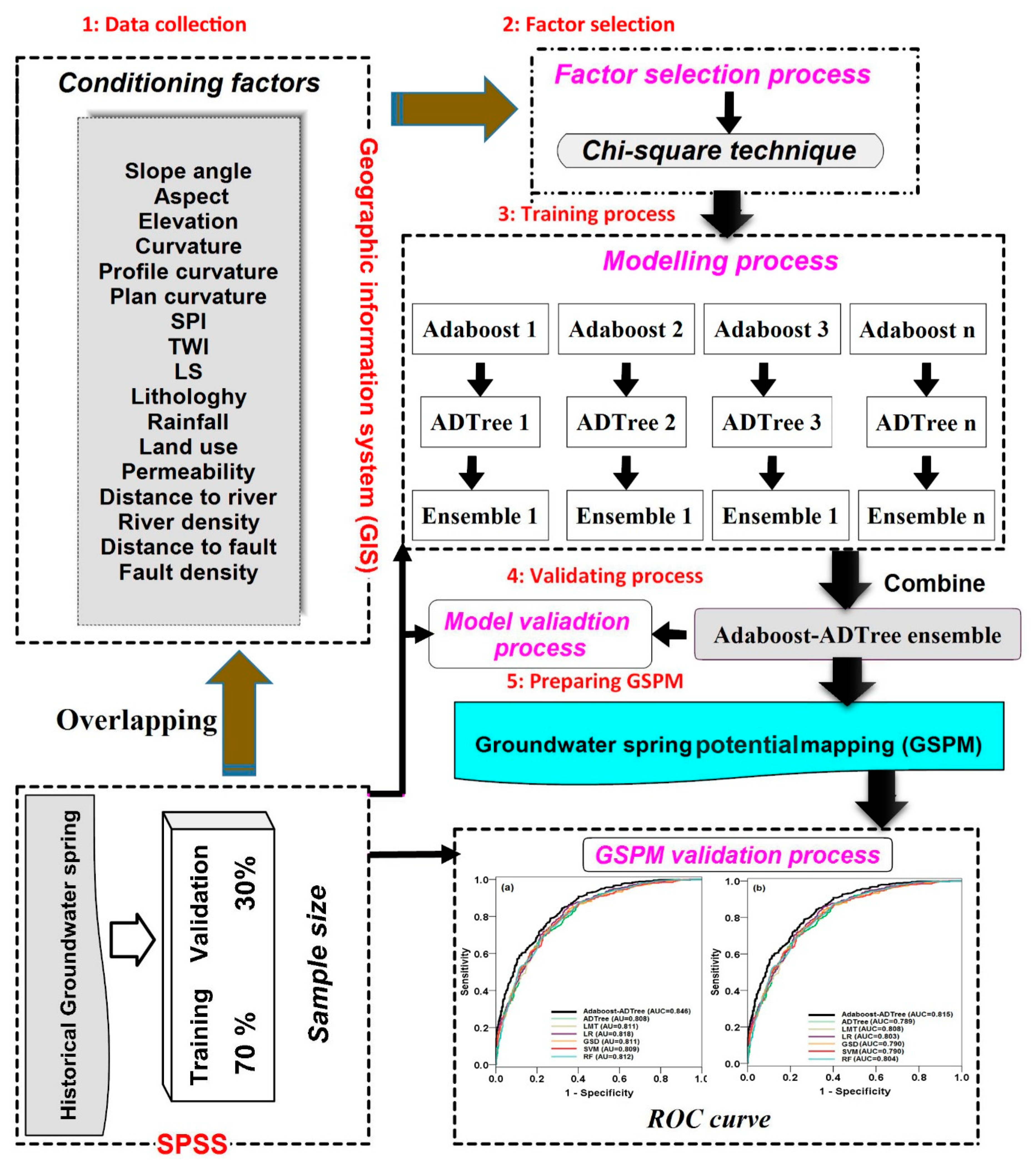
The Chilgazi watershed, which is located north of Sanandaj city, Kurdistan province, Iran, lies between 46°45′ to 46°57′ E longitudes and 35°25′ to 35°28′ N latitudes. This area covers an area of around 272 km2. The elevation of the study area ranges from 1550 to 2859 m (Figure 1). The Ghishlagh Dam is located at the outlet of the Chilgazi watershed. The average annual temperature is 14.2 °C; the average daily minimum temperature in winter is 6.5 °C, and the average daily maximum temperature in summer is about 37 °C. The average annual precipitation is 464.2 mm, such that it mainly occurs in December to April (more than 75%). The climate of the study area based on De-Marttone climatic system is classified as semi-arid [109]. Most of the area is covered by agricultural lands (23,465 ha) and rangelands (3768 ha). In addition, barren lands, pastures, residential areas, and gardens are other types of land use in the study area. The study area is geologically part of elevated Zagros (Northern Zagros) where joints, gaps, and faults have been created. Also, soil of the study area is mainly semi-deep with predominant sandy-loamy texture. Most of the study area has been covered by the Quaternary deposits, including andesite–basalt ( K v c ), Sanandaj shale ( K S S ), and limestone ( K u l ). In addition, surface water and groundwater are the two sources of water supply, where surface water is often used for irrigation purposes and groundwater is commonly utilized for agricultural production as well as domestic purposes.

3. Data Acquisition

3.1. Data Collection and Interpretation

The locations of springs were determined in three steps: (1) The initial locations of springs were acquired from the Iran Water Resources Management Company (IWRMC), recorded between 2008 and 2010; (2) these locations were overlaid on the topographic map with a scale of 1:25,000 in order to control the initial location; and (3) some springs were randomly checked by field surveying for the final confirmation of their locations. Table 1 illustrates some statistical measures of springs. Basically, the discharge (lit/s) of all springs ranged between 0.2 and 10. Additionally, the average water temperature of springs (T), electrical conductivity (EC), and potential of hydrogen (pH) were 14.812 °C, 364.688, and 7.525, respectively.
In this study, the target (dependent) variable is spring locations over the study area as binary coding (spring (1) and non-spring (0) locations); however, independent variables (conditioning factors) were selected, based on the literature and data availability. Accordingly, a total of 633 springs were recorded and detected, of which 70% (444) of spring locations were randomly utilized for training and the other (30% or 190) were considered for validation of models using SPSS software. In the modeling process, using machine learning the independent variables should be binary, such as spring and non-spring occurrences. The locations of springs in the study area were easily recorded by global position system (GPS); however, the non-spring locations were recorded randomly over the study area using the “create random point” tool in Arc GIS 10.2. It is assumed that these locations are free from springs and that they do not have enough potential for spring occurrence. Some researchers have used these techniques for modeling groundwater productivity [29,110,111]. Therefore, to construct the datasets, similar to the training sample size, 633 locations were randomly selected and also partitioned into 70% (training) and 30% (validation) for modeling and evaluation, respectively. All spring locations and conditioning factors were converted to pixel sizes of 20 × 20 m to construct the final dataset.

3.2. Groundwater Spring Conditioning Factors

Selecting the most relevant conditioning factors (geo-database), related to the occurrence of a spring, is a critical issue for GSPM. Hence, based on the literature review, 17 groundwater spring influencing factors were detected and classified into four groups: Topography (slope angle, curvature, slope aspect, plan curvature, elevation, profile curvature, and sediment transport index), hydrology (rainfall, sediment transport power (SPI), distance to river, topographic wetness index (TWI), and river density), geology (lithology, fault density, distance to fault, and permeability), and land cover (land use) factors (Table 2). To generate the thematic (slope angle, slope aspect, elevation, curvature, profile curvature, plan curvature, sediment transport index (STI), SPI, TWI, distance to rivers, and river density) maps, a digital elevation model (DEM) of the study area with 20 m spatial resolution was constructed from the topographic map (1:25,000 scale). Hence, for all the conditioning factors, a pixel size of 20 × 20 m was selected.

3.2.1. Topographic Factors

Slope angle was considered as a terrain feature to recognize groundwater conditions [112,113]. It affects the recharge through infiltration so that the more the slope angle is, the greater the infiltration and the recharge are [114]. Slope angle of the study area ranged from 10 to >40 degrees which was then classified into five classes, such as (1) 0–10; (2) 10–20; (3) 20–30; (4) 30–40; and (5) >40 (Table 2).
Slope aspect is a well-known conditioning factor of GSPM [12,13,22]. Slope aspect can affect hydrologic response, such as solar radiation, soil-water retention, soil porosity, hydraulic conductivity, snow ablation, evapotranspiration, water cycling, and vegetation communities [115,116,117,118,119]. Generally, in the northern hemisphere, north-facing slopes are colder and wetter than south-facing slopes, which are warmer and drier [120]. Therefore, the north-facing slopes have more potential for spring occurrence that indicates that groundwater is higher than at the other places. The slope aspect map of this area was derived from DEM with nine classes (Table 2), including Flat, North, Northeast, East, Southeast, South, Southeast, West, and Northwest.
Elevation is known as the height above the earth surface; it is related with climate and environment, thus affecting groundwater springs [121]. It can affect the weather and climate change, and can influence soil properties and vegetation communities [39]. Basically, the higher the elevation is, the more the potential of springs because of more rainfall in comparison to lower elevations. The elevation map of this study was extracted from DEM and classified into five classes, including (1) <1800; (2) 1800–1900; (3) 1900–2000; (4) 2000–2200; and (5) >2200 (Table 2).
Curvature generally has a negative relationship with groundwater recharge [13]. Thus, it is considered as a conditioning factor affecting groundwater spring [13]. The curvature map of the study area was generated in five categories: (1) ((−13.5)–(−2.24)); (2) ((−2.24)–(−0.661)); (3) ((−0.661)–(−0.394)); (4) >((−0.394)–(−1.66)); and (5) ((−1.66)–(−13.3)) (Table 2).
Plan curvature and profile curvature are the curvatures of a contour line formed by intersecting the surface with a horizontal plan and a vertical plan, respectively; thus, they affect groundwater springs [83]. Plan curvature describes the divergence and convergence of flow and it can affect the concentration of flow on the ground [122]. However, profile curvature can affect the pore water pressure, saturated and recharge resulting in the development of groundwater. The plan curvature map of study area was extracted from DEM and classified into five levels, such as (1) ((−7.78)–(−1.3)); (2) ((−1.3)–(−0.381)); (3) ((−0.381)–0.339); (4) >(0.339–1.45); and (5) (1.45–8.91) (Table 2). The profile curvature was also extracted from DEM and classified into five classes, including (1) ((−7.13)–(−1.46)); (2) ((−1.46)–(-0.450)); (3) ((−0.450)–0.141); (4) >(0.141–0.791); and (5) (0.791–7.89) (Table 2).
STI/low susceptibility (LS), as an important conditioning factor in the study of groundwater spring, shows the erosion power of overland streams due to two structural elements, including carrier content of alluvium flow and basin evolvement [123,124]. The STI is computed from the following equation:
S T I = ( A s 22.13 ) 0.6 ( sin β 0.0896 ) 1.3
where A s is the specific basin area (m2/m), and β the slope gradient [78]. In this study, the STI values of study area were divided into five classes, involving (1) 0–3.83; (2) 3.83–8.66; (3) 8.66–13.3; (4) 13.3–18.8; and (5) 18.8–42.5 (Table 2).

3.2.2. Hydrological Factors

Rainfall is a hydrologic process for recharging aquifers [125,126]. Groundwater potentiality increases as rainfall increases [114]. In this study, the mean annual rainfall data of ten meteorological stations were acquired from the I.R. of Iran Meteorological Organization (IRIMO). Rainfall in the study area ranged between 300 and >480 mm, which was then classified into seven classes, including (1) 300–340; (2) 340–360; (3) 360–380; (4) 380–400; (5) 400–440; (6) 440–480; and (7) >480 (Table 2).
SPI has been considered as one of the conditioning factors which contributes to groundwater springs [41,42]. Generally, the higher the SPI is, the higher the potential for spring occurrence because of having a higher water table. It was extracted DEM, where SPI values can be computed by the following equation [127]:
S P I = A s tan β
where A s is defined as the specific basin area, and β is defined as the local slope gradient in degree.
The SPI values ranged from 500 to 116,000 which were divided into five categories: (1) 0–500; (2) 500–1000; (3) 1000–1500; (4) 1500–2000; and (5) 2000–116,000 (Table 2).
TWI is an important conditioning factor for GSPM [13,128], as permeability and pore water pressure of materials are affected by water infiltration and soil strength [42]. It has been extensively used to describe the effect of topography on the size and location of saturated source areas which are prone to runoff generation. Basically, areas with higher TWI indicate also the higher potential for spring occurrence. The following equation was used for the TWI computation [129]:
T W I = L n ( A s tan β )
where A s is defined as the specific basin area, and tanβ is defined as the angle of slope at that point. The TWI values for the study area were classified into five classes: (1) 0.649–3.31; (2) 3.31–4.16; (3) 4.16–6.42; (4) 6.42–8.88; (5) 8.88–10.9 (Table 2).
Distance to rivers affects the moisture content of soil and rock on the slope, thus affecting groundwater springs [28]. This factor can affect the recharge process so that the shorter the distance from river, the higher the potential to infiltration in comparison to farther distance from the river networks [130]. According to the DEM of the study area, the multi-buffer values of rivers were generated with five classes: (1) 0–100; (2) 100–200; (3) 200–300; (4) 300–400; and (5) >400 (Table 2).
River density is considered as an important conditioning factor for GSPM [114], as when the drainage density is lower, the infiltration and recharge are greater [125,131]. The higher the drainage density is, the lower the infiltration and the higher the surface runoff are, which indicates that this factor has a reverse relationship with groundwater [131]. The river density of the study area varied from 0 to 0.00633 (km/km2) which was then divided into five categories: (1) 0–0.000744; (2) 0.000744–0.00169; (3) 0.00169–0. 00248; (4) 0. 00248–0.00337; and (5) 0.00337–0.00633 (Table 2).

3.2.3. Geological Factors

Lithology is related to both soil porosity and water permeability of aquifers [114,132]. In general, karst and fissured rock aquifers have lower capacity and specific storage of groundwater springs than sedimentary aquifers [114]. The lithology map of the area was constructed from the geological map at 1:100,000 scale collected from the Geological Survey & Mineral Exploitation of Iran (GSMEI). In this study, lithology was reclassified into ten classes, including (1) alluvial fan and terraces (Qt1 and Qt2); (2) alluvial deposits (Qal); (3) limestone (Kul, Kpf, and Kf1); (4) sandstone (Kvsl); (5) shale (Kss); (6) turbidite sequence (Ktsc); (7) conglomerate with intermediate of Sandston (Klt); (8) un-granulated conglomerate with shale and sandstone (Kco); (9) lava and tuff (Kvc and Kv); and (10) coarse-grained gabbro (gb) (Table 2).
Distance to fault is another vital factor for studying groundwater springs. This factor can affect infiltration so that the shorter the distance from the fault, the higher the potential to infiltration in comparison to farther distance from the river networks. Different types of faults can control the movement of groundwater springs on the geological structure of an area [15]. Faults of the study area were extracted from the geological map at 1:100,000 scale and distance to faults map was constructed with five categories, such as (1) 0–100; (2) 100–200; (3) 200–300; (4) 300–400; and (5) >400 (Table 2).
Fault density is described as the relationship between the sum of fault lengths in the pixel and the area of the corresponding pixel [121]. The areas with more faults, if they receive enough moisture and water, are also more likely to develop springs and develop aquifers than the areas with less faults. Therefore, these areas easily recharge the groundwater aquifers. The fault density of the study area was calculated from the geological map at 1:100,000 scale and was then divided into five classes: (1) 0–0.000418; (2) 0.000418–0.00114; (3) 0.00114–0.00185; (4) 0.00185–0.00267; and (5) 0.00267–0.00508 km/km2 (Table 2).
Permeability is one of the geological factors that affects the groundwater spring occurrence using discontinuity structures, such as joints, cracks, and faults. This factor was evaluated using expert knowledge and field surveys based on the lithological units. Eventually, the permeability map was classified into four categories, including very low, low, moderate, and high (Table 2).

3.2.4. Land Cover Factors

Land use affects infiltration and runoff, thus affecting GSPM [131]. Moreover, the development of groundwater spring resources is due to land use [133]. In this study, land use was generated from ETM+ satellite images in 2013 with different classes: (1) Woodland; (2) residential area; (3) barren land; (4) outcrop land; (5) range land; (6) dry farming land; and (7) farming land (Table 2).

4. Theoretical Background of Machine Learning Algorithms

4.1. Logistic Regression (LR)

The LR model has become a widely used and accepted model to analyze the binary outcome variables [134,135], describing both independent and dependent variables. In LR, the relationship between independent and dependent variables is nonlinear [136]. Thus, it was used to describe the relationship between spring occurrence and spring-affected factors, and can be expressed as follows:
p = 1 1 + e m
where p is defined as the probability of a spring occurrence, and m infers the linear combination of a set of spring-affected factors.

4.2. Logistic Model Tree (LMT)

LMT is a comprehensive approach, which combines a decision tree and linear logistic regression technique and takes advantages of them [137]. It has a high speed of learning process as a stage wise fitting process is applied to the structure of LMT [138].
Compared with a traditional decision tree, LMT employs the logistic regression functions to value the probability of each class, and applies the LogitBoost algorithm to build the logistic regression functions at the nodes of a tree. It uses the well-known CART algorithm [139] for pruning. A posterior probability for each class is determined as follows:
P ( c l a s s = c | x ) = e ( H c ( x ) ) n = 1 C e ( H n ( x ) )
where H c ( x ) is transformed such that c = 1 c H c ( x ) = 0 , and c is the number of classes.

4.3. Stochastic Gradient Descent (SGD)

It is necessary to introduce a simple supervised learning set-up before introducing a stochastic gradient descent approach. An arbitrary input x and a scalar output y make up an example z ( x , y ) . In this study, x is the spring-affected factor, and y is the spring and non-spring. There is a function h ( y , y ) which measures the cost of predicting y when the actual answer is y , and a function f θ ( x ) parameterized by a weight vector θ is chosen. Then we seek the function f which can minimize the loss D ( z , θ ) = h ( f θ ( x ) , y ) averaged on the examples:
R ( f ) = h ( f θ ( x ) , y ) d P ( z )
R n ( f ) = 1 n i = 1 n h ( f ( x i ) , y i )
where R ( f ) measures the generalization performance, and R n ( f ) measures the training dataset performance. The SGD algorithm is a drastic simplification without the gradient of R n ( f θ ) [140]. This model can directly optimize the expected risk, since the examples are randomly withdrawn from the ground truth distribution.

4.4. Support Vector Machine (SVM)

SVMs are a set of optimal separating hyper plane-based machine learning techniques [141,142]. The goal of the SVM model is to minimize both model complexity and error test. In this case, our aim is to discriminate between spring and non-spring. SVMs have separate examples in different classes using the following function:
h ( x ) = { w , x } + c = i = 1 N ( w i x i ) + c = 0
where x represents the independent spring-affected factors, w represents the vector of weight, and c is a constant.

4.5. Alternating Decision Tree (ADTree)

ADTree is a generalization of decision trees, combining the boosting algorithm and decision tree [143,144]. ADTree graphical rule sets form leaves of the tree. Each branch of the tree ends in an outcome and goes for another rule until it reaches the root [145]. The path continues with all of the node children when reaching a prediction node. Once a set of instances reaches the leaf node, a classification is established over them. For numerical prediction purposes, the leaf nodes would be the numeric outcomes for which the values are computed, based on a weight as a contribution of that node to the final outcome. The final prediction probability is formed from the summation of all the weights contributing to the root of the tree [144].

4.6. Random Forest (RF)

Random forest (RF), which was first developed by Breiman [146], is a non-parametric model and an extension of the classification and regression trees (CART) algorithm. It produces many classification trees to enhance the prediction performance of the model. In the RF model, the splitting process of the tree at each node is done using a randomized subset of the variables. The output of the RF model is obtained by the averaging of the results of all trees [147]. The RF model is constituted by numerous trees, that each tree is produced by bootstrap samples using the out-of-bag (OOB) error. The OOB is an unbiased estimate of the generalization error that has been explained and interpreted by Breiman [146]. This technique (bootstrap by OOB error) has advantages, including: (1) Prevention of over-fitting during modeling by training dataset; (2) decreasing the bias and variance of the training dataset because of a large number of trees; (3) decreasing the correlation among the individual trees when the diversity of forest arises by using limit variables; (4) robust error estimates using the OOB data; and (5) achieving a higher prediction performance (Wiesmeier et al. [148]). Breiman [146] and Liaw and Wiener [149] have explained the mathematical equations of the RF in detail. In this study, the RF was used to analyze the relationship between groundwater spring locations as binary dependent variables (groundwater spring locations (1) and groundwater on-spring locations (0)), and independent variables such as slope angle, curvature, slope aspect, plan curvature, elevation, profile curvature, and sediment transport index, rainfall, sediment transport power (SPI), distance to river, topographic wetness index (TWI), and river density, lithology, fault density, distance to fault, permeability, and land use. The RF was used to obtain a probability value for each pixel of the study area to prepare groundwater spring potential mapping.

4.7. AB Learning Ensemble Techniques

As a kind of ensemble algorithm, AB constructs a composite classifier by sequentially training classifiers. The algorithm was first proposed by Freund and Schapire to improve the performance of weak classifiers [150].
This algorithm assigns a weight to each factor in the training dataset C . At the same time, each sample in the training dataset C is assigned an equal weight ( 1 / n ); therefore, in the first process, all of the samples have the same opportunity to be selected. It takes T rounds of training-based learners with T different training sample groups G t ( t = 1 , 2 , T ) to generate the AB model, and this process continues until reaching a terminated condition [151].

“AB–ADTree” Model

In this study, we combined a decision tree classifier, Alternating Decision Tree (ADTree), with a Meta/ensemble classifier, AB—named “AB–ADTree”—in order to spatially predict springs. The framework of the proposed ensemble model is shown in Figure 2. Basically, the GSPM using the proposed model was performed in five steps: (1) Data collection and interpretation; (2) selecting the most conditioning factors using the chi-square technique in modeling; (3) training the AB–ADTree ensemble model; (4) validating and comparing spring models; and (5) preparing groundwater potential maps.

4.8. Accuracy Assessment (Validation) and Comparison of Methods

The most important issue in introducing a novel model, and also comparing some methods with each other, is to assess the performance (classifier performance or model validation). Validation as an essential process in any natural hazard phenomenon which reflects the predictive power of a model is related to the comparison of model performance with a real-word dataset [152].

4.8.1. Statistical Measures

Generally, there are statistical criteria for validating machine learning models [153]; however, in this study, six statistical index-based measures, including sensitivity (recall), root mean square error (RMSE) specificity, negative predictive value (NPV), accuracy, positive predictive value (PPV), and the area under the receiver operating characteristic (ROC) curve (AUROC), were used to evaluate the predictive capability of the proposed model with other benchmark models. Most of the above-mentioned criteria were computed based on the contingency table (confusion matrix), which is shown in Table 3 where TP is the number of pixels that are correctly classified as positive (springs) predictions, while the number of pixels that are correctly classified as negative (non-springs) predictions was TN. FP and FN are the pixels that were incorrectly classified as positive (springs) and negative (non-springs) predictions, respectively.
More specifically, sensitivity (recall) is the number of correctly classified springs per total predicted springs, while specificity is defined as the number of incorrectly classified springs per total predicted non-springs. Accuracy (efficiency) is the proportion of spring and non-spring pixels which are correctly classified [123,126,154]. PPV and NPV are the probabilities of pixels that were correctly classified as springs and non-springs, respectively. RMSE indicates the error metric between the estimated and observed values [154]. A smaller RMSE indicates a better performance of the models [155]. The statistical index-based measures were calculated using following equations:
Sensitivity = T P T P + F N
Specificity = T N T N + F P
Accuracy   = TP + TN TP + TN + FP + FN
P P V = T P T P + F P
N P V = T N T N + F N
RMSE = 1 n i = 1 n ( X p r e d i c t e d X a c t u a l ) 2
where n is defined as the total sample in a dataset; X p r e d i c t e d is the predicted value in the dataset; and X a c t u a l is the actual (output) value.

4.8.2. Receiver Operating Characteristics Curve (ROC)

The receiver operating characteristic curve was first suggested by Spackman [156] to evaluate the performance of empirical learning systems [105]. It is another statistical tool which is a popular and highly useful graphical representation of evaluation of the model performance [157]. Graphically, it is plotted on two axes (two-dimensional), including x-axis labeled with true positive rate or sensitivity ( TP   =   TP / ( TP   +   FN )   =   TP / N ) and y-axis labeled with false positive rate or 100-specificty ( FP   =   FP / ( FP   +   TN )   =   FP / N ) [158]. In the machine learning techniques, ROC is a flexible and robust framework for evaluating the performance of classifier [159,160]. The ROC is quantitatively defined using the area under the curve (AUC), which is widely used as a popular measure in the classification of performance [153]. It is more applicable over other performance metrics when no threshold is fixed and applied to the scores, and is invariant to changes in cost and class distribution [161]. In the optimal classifier (perfect model), the AUC has a value of 1, while for a random classifier (inaccurate model) a value of 0.5 is obtained [162].

4.8.3. Statistical Assessment

In order to check the statistical difference between the two groundwater spring potential models, Friedman and Wilcoxon rank tests were used in this study, where Friedman test indicates that there is no significant difference between the two models and Wilcoxon rank test indicates that statistical difference is observed between the two models. Friedman test, as a non-parametric test, is based on the null hypothesis that the performances of groundwater spring models is different at the significance level of α = 0.05. The p-value was used to evaluate this hypothesis, as if a hypothesis is likely true, then the null hypothesis is rejected, which indicates a significant difference between the two models and vice versa [58]. However, the Friedman test cannot perform pairwise comparisons between the models. Therefore, the Wilcoxon sign-rank was used to evaluate the systematic pairwise differences between the models. In general, the null hypothesis is rejected if the p-value is <0.05 and the z-value is >(−1.96 and +1.96) [58].

4.9. Selection of Training Factors Using Chi-Square Technique

The chi-square statistical test was employed to select training factors among attributes (conditioning factors). It is a traditional statistic to measure the relationship between two variables (factors) in the contingency table. The chi-square test compared the observed and expected frequencies of variables, so that the greater the chi-square for a variable, the higher the relationship. The results of this test were obtained using the following basic functions:
χ 2 = ( x i j E i j ) 2 E i j
E i j = ( x i x j ) N
where E i j is the expected value for each cell in the contingency table. We used the chi-square statistical test to specify the independence between spring and no-spring locations with other conditioning factors. If χ 2 equaled 0, it was assumed that there was no association between them and the conditioning factor would be eliminated from the model training.

5. Results and Analysis

5.1. Groundwater Spring Conditioning Factor Analysis

Both models and input data affect the quality of GSPM results [15]. The influence of conditioning factors on groundwater spring occurrence is different, such that some of them may reduce the model accuracy. The main step in the spatial GSPM is the selection of suitable factors and the elimination of irrelevant conditioning factors to find the most reliable database. In this study, the chi-square attribute evaluation (CSAE) technique, which is one of the most efficient and popular methods [163], with 10-fold cross validation for the training dataset was used to assess the prediction capability of conditioning factors. Results of the chi-square test (Figure 3) show that the most important conditioning factors for groundwater spring potential were TWI (AM = 98.598), followed by distance from river (AM = 97.73), SPI (AM = 83.736), slope angle (AM = 77.624), plan curvature (AM = 67.59), STI (AM = 55.488), Land use (AM = 48.146), geology (AM = 44.805), curvature (AM = 31.404), stream density (AM = 31.830), rainfall (AM = 30.530), elevation (AM = 30.304), and permeability (AM = 17.481).

5.2. Model Training and Assessment

The results of seven models, namely AB–ADTree, ADTree, SGD, LMT, SVM, and LR, constructed for groundwater spring potential prediction using the selected conditioning factors and training dataset are shown in Table 4. The training dataset was used to train the models. In the training dataset, the hybrid model (AB–ADTree) had the highest performance based on PPV, NPV, sensitivity, specificity, accuracy, kappa, AUC, and RMSE criteria. This shows that the hybrid model outperformed other individual models. AB–ADTree had the highest PPV (0.815), followed by ADTree (0.751), RF (0.749), LMT (0.746), LR (0.746), SVM (0.745), and SGD (0.724), indicating that these models in 81.5%, 75.1%, 74.6%, 74.6%, 74.5%, and 72.4% of the cases correctly classified pixels in the groundwater spring occurrence class.
Regarding NPV, AB–ADTree had the highest performance (0.785), demonstrating that 78.5% of pixels were correctly classified as the non-groundwater potential occurrence class, followed by RF (0.748), SGD (0.745), SVM (0.739), LR (0.738), LMT (0.736), and ADTree (0.718). AB–ADTree obtained the highest sensitivity (0.775), showing that 77.5% of the groundwater spring occurrence pixels were correctly classified as the groundwater spring occurrence class, followed by RF (0.748), SGD (0.757), SVM (0.736), LR (0.734), LMT (0.730), and ADTree (0.698). The highest specificity (0.824) of the AB–ADTree model showed that 82.4% of the non-groundwater spring occurrence pixels were correctly classified as the non-groundwater spring occurrence class, followed by ADTree (0.768), LMT (0.755), RF and LR (0.750), SVM (0.748), and SGD (0.712). The AB–ADTree model also acquired the highest performance (0.800) evaluated by the accuracy criterion, followed by RF (0.749), LMT, SVM and LR (0.742), SGD (0.734), and ADTree (0.733). Results of RMSE demonstrated that AB–ADTree had the lowest error (0.375), followed by LR (0.417), LMT and SVM (0.418), ADTree (0.424), and SGD (0.515). Regarding AUC, the hybrid model of AB–ADTree had the highest AUC (0.881), followed by RF (0.818), ADTree (0.817), LR (0.816), SVM and LMT (0.815), and SGD (0.675). The findings prove that the designed hybrid model showed the highest performance in groundwater spring potential prediction based on all criteria used in the training phase of modeling in this research.

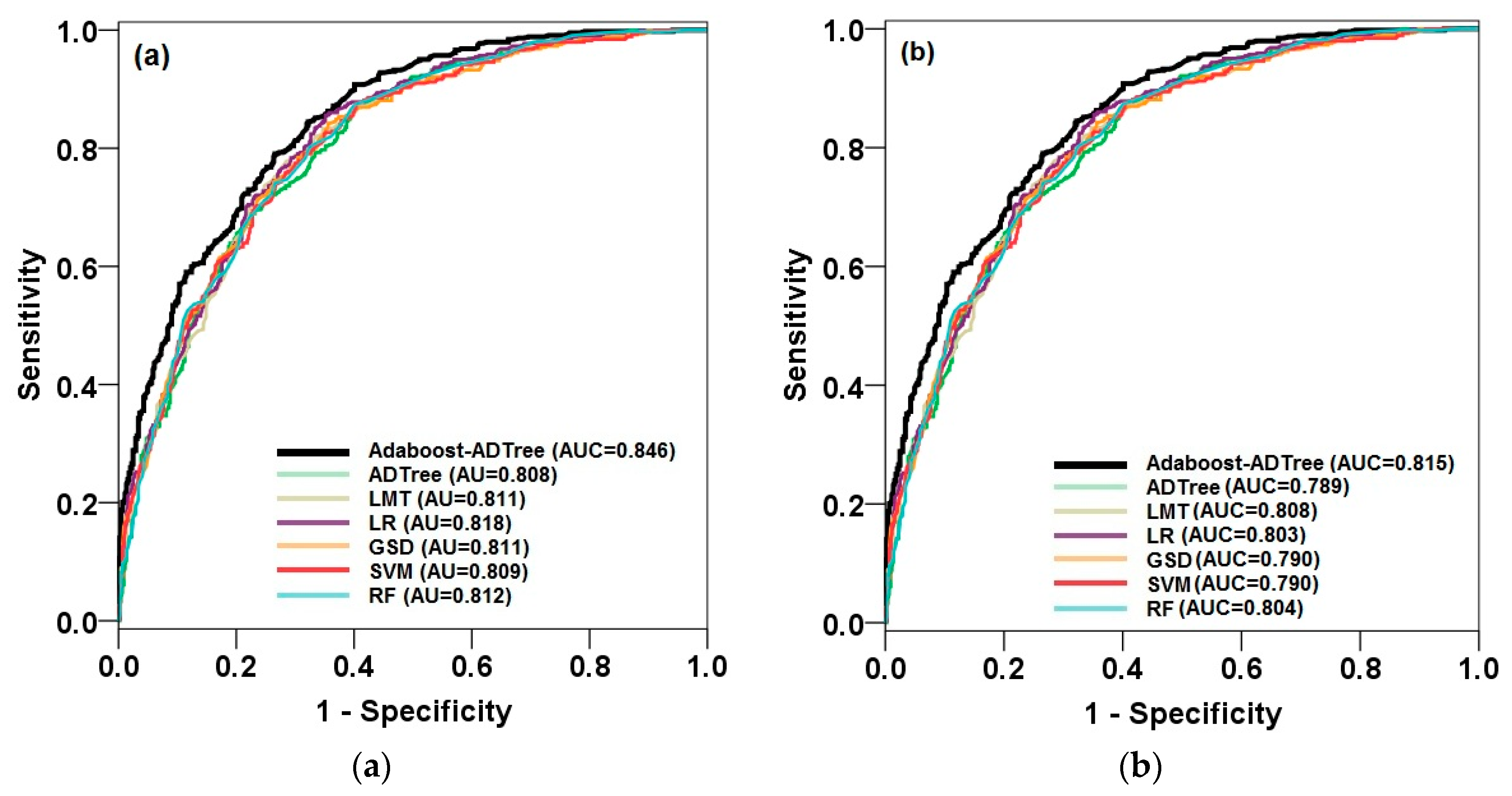
5.3. Models Validation and Comparison

Validating or testing the dataset that was not used in the training step was employed for the prediction capability of seven models for the identification of groundwater spring potential and their comparison. Results of the prediction power of the models are shown in Table 5. The hybrid model showed a higher performance than other individual models in the testing phase for most of the evaluation methods. The AB–ADTree model had the highest probability to correctly classify pixels of the groundwater spring potential classes (73.2%), followed by LR (73.1%), LMT (72.6%), RF and SVM (72.4%), SGD (71.4%), and ADTree (70.8%), whereas SGD showed the highest probability to correctly classify pixels to non-spring potential (76.5%), followed by LR (75.8%), RF and SVM (75.7%), LMT (75.4%), AB–ADTree (75.3%), and ADTree (73.6%). The SGD model classified 78.9% of the spring occurrence pixels correctly as spring potential classes showed the highest sensitivity, followed by RF, SVM, and LR (77.4%), LMT (76.8%), AB–ADTree (76.3%), and ADTree (75.3%), whereas the AB–ADTree model classified 72.1% of the non-spring occurrences pixels correctly as non-spring potential classes which had the highest specificity, followed by LR (71.6%) and LMT (71.1%), RF and SVM (70.5%), ADTree (68.9%), and SGD (68.4%). The highest classification accuracy belonged to AB–ADTree (74.2%), followed by RF, LMT, and SVM (73.9%), SGD (73.7%), ADTree (72.1%), and LR (65.4%). The ADTree model had the lowest RMSE (0.375), followed by AB–ADTree (0.419), RF (0.413), SVM (0.425), LMT and LR (0.426), and finally SGD (0.513). The AB–ADTree model demonstrated the highest AUC (0.829), followed by RF (0.809), SVM (0.807), LR (0.805), LMT (0.803), ADTree (0.790), and SGD (0.675). The results reveal that the designed hybrid model of AB–ADTree performed much better than other studied models in the validation phase of modeling in this research.

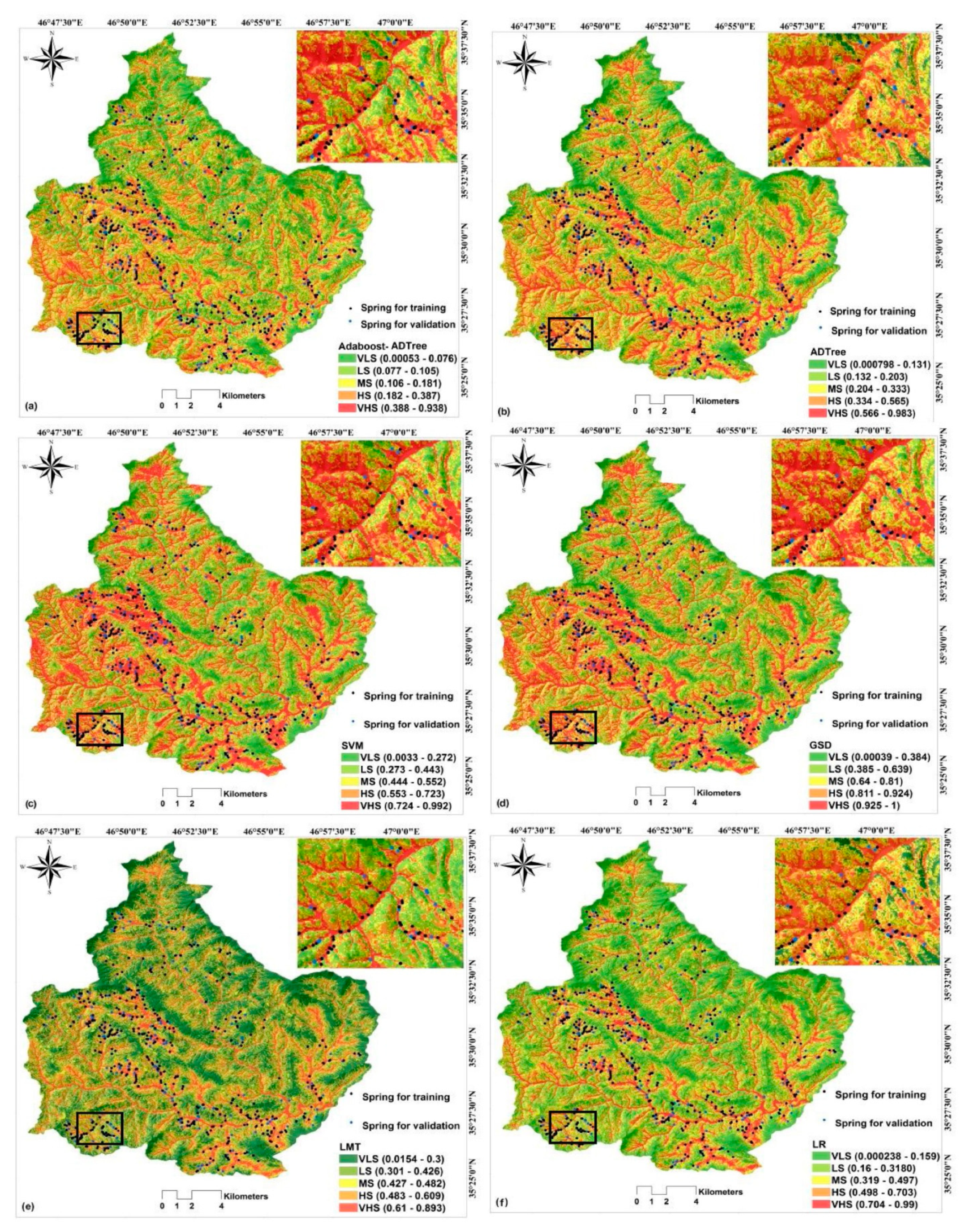
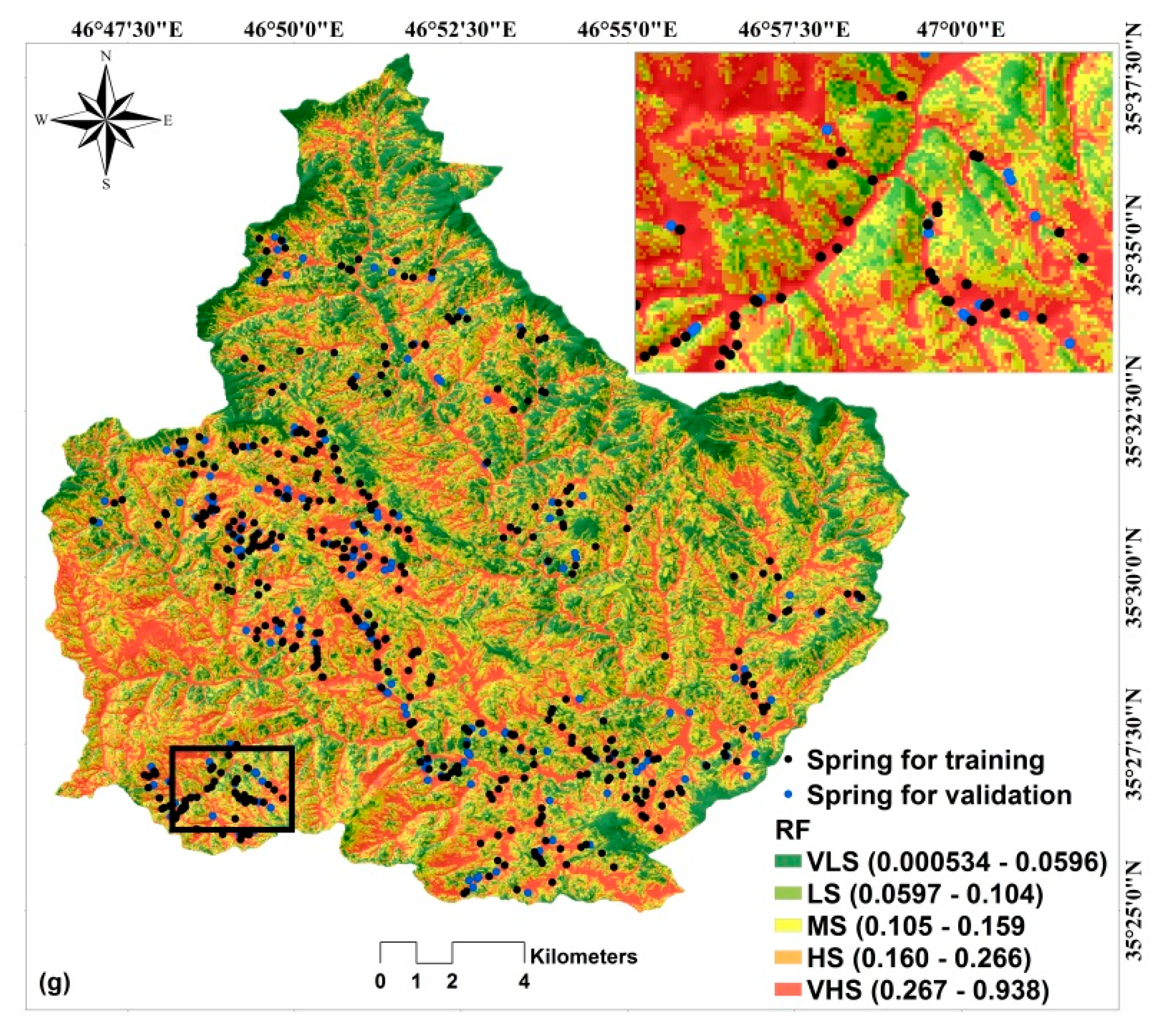
5.4. Groundwater Spring Potential Mapping

After successful modeling in the training phase, the AB–ADTree, ADTree, SGD, LMT, SVM LR, and RF models were used to calculate the groundwater spring potential index for all pixels. Exported in GIS format, these indices were visualized by means of five susceptibility classes of groundwater spring potential, including very low susceptibility (VLS), low susceptibility (LS), moderate susceptibility (MS), high susceptibility (HS), and very high susceptibility (VHS). Different classification methods can be used for the classification of potential indices, such that in the current research, the quantile method was used, based on the literature review and the nature of data.
AB–ADTree, ADTree, SGD, LMT, SVM, LR, and RF were used for preparing the GSPM at the Chilgazi watershed. Two main steps for generating groundwater spring potential indices and reclassifying these indices were used for the preparation of maps. In the first step, a unique susceptibility index was assigned to each pixel of the research area and in the second step, these indices were classified into different classes using the quantile method [164], resulting in six maps by six models (Figure 4). Results show that the west part of the Chilgazi watershed showed higher potential for spring occurrence than other parts.

5.5. GSPM Validation and Comparison

The reliability of these spring potential maps was evaluated using success and prediction rates (Figure 5). For this purpose, the training dataset and validation dataset were overlaid on the GSPM and the AUC was calculated for training and validation datasets. According to Figure 5a (success rate curve), results indicate that the hybrid model, AB–ADTree, had the highest goodness-of-fit base on the training dataset (AUC = 0.846). This implies that, at the present condition of the study area, this model could appropriately distinguish the areas with high groundwater spring potential. On the other hand, most of the spring locations were located in high and very high potential areas of the map. It was followed by the RF (AUC = 0.812), LR (AUC = 0.818), LMT equal to SGD (AUC = 0.811), and SVM (AUC = 809) models. This means that the ability of the RF model to classify and detect the areas with high groundwater potential is higher than that of the LR, LMT, SGD, and SVM models.
For prediction rate or model validation that was built using the validation dataset, the highest AUC belonged to AB–ADTree (0.815), followed by LMT (0.808), RF (0.804), LR (0.803), and SGD and SVM (0.790). Therefore, the map resulting from the novel hybrid model was ranked as the most accurate and reliable model among others. Yesilnacar [165] classified the success of a model using a quantitative–qualitative relationship. Basically, if a model has an AUC between 0.9 and 1, its prediction accuracy is excellent, and for 0.8–0.9, 0.7–0.8, 0.6–0.7, and 0.5–0.6, the prediction accuracy is very good, good, average, and poor, respectively. Regarding this classification and Figure 5b, the findings indicate that all machine learning models had a good prediction power in groundwater potential mapping, although the ability of the AB–ADTree, LMT, RF, and LR models for groundwater was relatively higher than the ADTree, SGD, and SVM models in the study area.

5.6. Similarities Between Prediction Power of Models

The seven models used in this study showed very good to good prediction abilities, while it remained to be determined whether there were statistically significant differences between them or not. The Freidman test was used at the significance level of 5% for this purpose (Table 6). The mean ranking of the seven models for the study area is shown in Table 6. Results reveal that because the p-value was 0.000, i.e., less than 0.05, the null hypothesis was rejected, indicating that there were statistically significant differences between the six models.
The Freidman test was not able to provide comparisons between the seven models. Therefore, the Wilcoxon sign-rank test was carried out to check the statistical significance of pairwise differences between the GSPM models. In this test, there was a pairwise comparison between the models at the 5% significant level. The p-value and z-value were used to evaluate the statistically significant differences between models. The results can be seen in Table 7. Because the p-value in all of the pairwise comparisons was less than 0.05 (0.000) and the z-value exceeded the z critical values (from −1.96 to +1.96), the null hypothesis was rejected, implying that the performances of the seven GSPM models were significantly different from each other.

6. Discussion

Recognizing the areas that have enough potential for groundwater exploration based on the spring density can be considered as one of the significant areas for water resources management, especially in semi-arid watersheds such as Chilgazi in the case study. Therefore, machine learning and ensemble techniques can be used as alternative and effective tools for preparing GSPM due to their ability and flexibility. This study applied and extended a hybrid machine learning algorithm, AB–ADTree, for this purpose, and the results were compared and validated based on statistical metrics and also some soft computing benchmark models. The factor selection using the chi-square attribute evaluation (CSAE) technique concluded that among 17 conditioning factors, only 13 factors were more significant and were considered for modeling—in which TWI was the most important factor. TWI indicates topographic wetness of the ground surface, and the higher the TWI is, the higher the probability of the water table to be closer to the ground surface. Springs occur in regions where the water table reaches ground surface. Naghibi and Dashtpagerdi [166] reported that according to the generalized cross validation technique TWI, slope angle and fault density were more important factors for GSPM in their study area. Additionally, some conditioning factors, including aspect, profile curvature, permeability, fault density, and distance to fault, were removed from the modeling in the training phase due to having zero chi-square values. There are two reasons for that: (i) The removed conditioning factors were maybe not contributing to explaining the spatial distribution of springs in the study area; (ii) it is probable that the cartography or method used for extracting the removed conditioning factors did not properly reflect them.
Results of modeling depict that the proposed ensemble model and benchmark machine learning models had satisfactory performances for groundwater spring potential mapping. The area under the ROCs illustrates that all models had an AUC from 0.790 to 0.815, indicating that although all models had high performance and prediction accuracy, the proposed model, AB–ADTree, outperformed and outclassed the other benchmarks models (ADTree, SGD, LR, LMT, SVM, and RF). In this line, this model had acceptable results in the other fields of the environment, such as groundwater well potential mapping [166], ecological modeling [167], landslide susceptibility modeling [168], and flood susceptibility modeling [169,170]. The findings pinpoint that the AB–ADTree ensemble model had a better fit to the training dataset during the modeling process, and then it had high prediction accuracy. In other words, adaptive boosting, known as AdaBoost, randomly divided the training dataset into some sub-training datasets. Then, on each dataset, the ADTree was employed and, finally, an output was obtained based on a weighted sum of all ADTree base performed models [171]. This process improved the goodness-of-fit and prediction accuracy of the ADTree by decreasing the over-fitting, and also errors, in training dataset [94,172,173].
Among benchmark machine learning models, the RF model had the highest prediction accuracy (AUC = 0.809), followed by the LMT, LR, SGD, SVM, and ADTree models. The LMT is one of the decision tree classifiers that is a combination of linear logistic regression model and a decision tree classifier that, in this study, had higher performance. On the other hand, the LR, SVM, and SGD models are based on the equation function to obtain the weight for each conditioning factor to spatially predict the groundwater potential. The results were obtained for the current study area, although the results may be different in other regions. This conflict is reflected by the uncertainties in the modeling process due to data and model selection. In other words, data (conditioning factors) are different from one region to another and it makes a different result during modeling. Additionally, the result of a model is totally different with another model in a given region with similar conditioning factors. Hence, each model should be tested and evaluated based on its conditions, and the best model with the highest predictive power should be selected. Meanwhile, the main goal was to reach a high-precision groundwater potential map that will allow to identify areas with high groundwater aquifers in the future to use in a critical condition, such as drought. Therefore, we tested the proposed model and other models for GSPM and it was confirmed to use in other environmental regions with similar conditions with more caution and requirements.

7. Conclusions

Springs, as groundwater resources, are important for many sectors, such as domestic consumption and agriculture in arid and semi-arid areas of the world. Sometimes, several families or villagers depend heavily on a spring; therefore, their spatial modeling is necessary. Different approaches can be taken for this type of modeling. We designed a hybrid machine learning approach called AB–ADTree to deal with this issue. Hydrological factors, including TWI, distance to river, and SPI, among others, such as topographic, geological, and land cover factors, were first evaluated as the most affecting conditioning factors for GSPM based on the chi-square attribute evaluation (CSAE) factor selection technique. This indicates that these factors can be applied to explore groundwater in the study area and similar areas in semi-arid regions.
To model GSPM, we selected the ADTree algorithm, and its ensemble was then applied based on the AB algorithm. This resulted in designing a hybrid machine learning model, AB–ADTree, to spatially predict groundwater spring locations in the Chilgazi watershed, Kurdistan province, Iran. The efficiency of this approach was verified by applying several soft computing benchmark algorithms, such as SGD, LMT, LR, SVM, and RF. The hybrid model was successfully trained and evaluated such that it acquired the highest rank of testing criteria, including PPV, NPV, sensitivity, specificity, accuracy, RMSE, and AUC, in both training and validation datasets. GSPM maps were generated by all of the applied models and evaluated by AUROC. The hybrid generated model had the highest prediction accuracy in comparison to other models. The Friedman and Wilcoxon rank statistical tests were used for further confirmation of the results. The findings indicate that the hybrid model, AB–ADTree, can be considered as a promising technique for the mapping of groundwater potential that has been overcome based on the study area conditions, and it is recommended that for other regions, it should be further tested and evaluated. Moreover, it can be useful for decision makers, planners, managers, and government agencies for the sustainable management of ground water resources.

Author Contributions

D.T.B., A.S., K.C., H.S., B.P., B.T.P., V.P.S., W.C., K.K., B.B.A., and S.L. contributed equally to the work. A.S., K.C., and H.S. collected field data and conducted the groundwater spring mapping and analysis. A.S., K.C., H.S., V.P.S., W.C., and K.K. wrote the manuscript. D.T.B., B.P., B.T.P., V.P.S., B.B.A., and S.L. provided critical comments in planning this paper and edited the manuscript. All the authors discussed the results and edited the manuscript.

Funding

This research was supported by the Basic Research Project of the Korea Institute of Geoscience, Mineral Resources (KIGAM) funded by the Minister of Science and ICT and Universiti Teknologi Malaysia (UTM) based on Research University Grant (Q. J130000.2527.17H84).

Conflicts of Interest

The authors declare no conflict of interest.

References

  1. Ayazi, M.H.; Pirasteh, S.; Arvin, A.; Pradhan, B.; Nikouravan, B.; Mansor, S. Disasters and risk reduction in groundwater: Zagros Mountain Southwest Iran using geoinformatics techniques. Disaster Adv. 2010, 3, 51–57. [Google Scholar]
  2. Neshat, A.; Pradhan, B.; Pirasteh, S.; Shafri, H.Z.M. Estimating groundwater vulnerability to pollution using a modified DRASTIC model in the Kerman agricultural area, Iran. Environ. Earth Sci. 2014, 71, 3119–3131. [Google Scholar] [CrossRef]
  3. Banks, D.; Robins, N.; Robins, N. An Introduction to Groundwater in Crystalline Bedrock; Norges geologiske undersøkelse: Trondheim, Norway, 2002. [Google Scholar]
  4. Saraf, A.; Choudhury, P. Integrated remote sensing and GIS for groundwater exploration and identification of artificial recharge sites. Int. J. Remote Sens. 1998, 19, 1825–1841. [Google Scholar] [CrossRef]
  5. BGR. Federal Institute for Geosciences and Natural Resources. Available online: http://www.bgr.bund.de (accessed on 12 July 2011).
  6. Arkoprovo, B.; Adarsa, J.; Prakash, S.S. Delineation of groundwater potential zones using satellite remote sensing and geographic information system techniques: A case study from Ganjam district, Orissa, India. Res. J. Recent Sci. 2012, 9, 59–66. [Google Scholar]
  7. Rahmati, O. An Investigation of Quantitative Zonation and Groundwater Potential (Case Study: Ghorveh-Dehgolan plain). Master’s Thesis, Tehran University, Tehran, Iran, 2013. [Google Scholar]
  8. Ghayoumian, J.; Saravi, M.M.; Feiznia, S.; Nouri, B.; Malekian, A. Application of GIS techniques to determine areas most suitable for artificial groundwater recharge in a coastal aquifer in southern Iran. J. Asian Earth Sci. 2007, 30, 364–374. [Google Scholar] [CrossRef]
  9. Abbaspour, K.C.; Faramarzi, M.; Ghasemi, S.S.; Yang, H. Assessing the impact of climate change on water resources in Iran. Water Resour. Res. 2009, 45, 1–16. [Google Scholar] [CrossRef]
  10. Zarghami, M.; Abdi, A.; Babaeian, I.; Hassanzadeh, Y.; Kanani, R. Impacts of climate change on runoffs in East Azerbaijan, Iran. Glob. Planet. Chang. 2011, 78, 137–146. [Google Scholar] [CrossRef]
  11. Hosseini, M.; Ghafouri, A.M.; Amin, M.; Tabatabaei, M.; Goodarzi, M.; Abde Kolahchi, A. Effects of land use changes on water balance in Taleghan Catchment, Iran. J. Agric. Sci. Technol. 2012, 14, 1161–1174. [Google Scholar]
  12. Rahmati, O.; Samani, A.N.; Mahdavi, M.; Pourghasemi, H.R.; Zeinivand, H. Groundwater potential mapping at Kurdistan region of Iran using analytic hierarchy process and GIS. Arab. J. Geosci. 2015, 8, 7059–7071. [Google Scholar] [CrossRef]
  13. Oh, H.J.; Kim, Y.S.; Choi, J.K.; Park, E.; Lee, S. GIS mapping of regional probabilistic groundwater potential in the area of Pohang City, Korea. J. Hydrol. 2011, 399, 158–172. [Google Scholar] [CrossRef]
  14. Zabihi, M.; Pourghasemi, H.R.; Pourtaghi, Z.S.; Behzadfar, M. GIS-based multivariate adaptive regression spline and random forest models for groundwater potential mapping in Iran. Environ. Earth Sci. 2016, 75, 665. [Google Scholar] [CrossRef]
  15. Moghaddam, D.D.; Rezaei, M.; Pourghasemi, H.; Pourtaghie, Z.; Pradhan, B. Groundwater spring potential mapping using bivariate statistical model and GIS in the Taleghan watershed, Iran. Arab. J. Geosci. 2015, 8, 913–929. [Google Scholar] [CrossRef]
  16. Kumar, U.; Kumar, B.; Mallick, N. Groundwater Prospects Zonation Based on RS and GIS Using Fuzzy Algebra in Khoh River Watershed, Pauri-Garhwal District, Uttarakhand, India. Glob. Perspect. Geogr. 2013, 1, 37–45. [Google Scholar]
  17. Israil, M.; Singhal, D.C.; Kumar, B.; Rao, M.S.; Verma, K. Groundwater resources evaluation in the Piedmont zone of Himalaya, India, using Isotope and GIS techniques. J. Spat. Hydrol. 2006, 6, 105–119. [Google Scholar]
  18. Kumar, B.; Kumar, U. Integrated approach using RS and GIS techniques for mapping of ground water prospects in Lower Sanjai Watershed, Jharkhand. Int. J. Geomat. Geosci. 2010, 1, 587–598. [Google Scholar]
  19. Kumar, A.; Sharma, H.C.; Kumar, S. Planning for replenishing the depleted groundwater in upper Gangetic plains using RS and GIS. Indian J. Soil Conserv. 2011, 39, 195–201. [Google Scholar]
  20. Thilagavathi, N.; Subramani, T.; Suresh, M.; Karunanidhi, D. Mapping of groundwater potential zones in Salem Chalk Hills, Tamil Nadu, India, using remote sensing and GIS techniques. Environ. Monit. Assess. 2015, 187, 164. [Google Scholar] [CrossRef]
  21. Jha, M.K.; Bongane, G.M.; Chowdary, V.M.; Cluckie, I.D.; Chen, Y.; Babovic, V.; Konikow, L.; Mynett, A.; Demuth, S.; Savic, D.A. Groundwater potential zoning by remote sensing, GIS and MCDM techniques: A case study of eastern India. In Proceedings of the Symposium JS.4 at the IAHS & IAH Convention, Hyderabad, India, 6–12 September 2009; pp. 432–441. [Google Scholar]
  22. Ozdemir, A. Using a binary logistic regression method and GIS for evaluating and mapping the groundwater spring potential in the Sultan Mountains (Aksehir, Turkey). J. Hydrol. 2011, 405, 123–136. [Google Scholar] [CrossRef]
  23. Elbeih, S.F. An overview of integrated remote sensing and GIS for groundwater mapping in Egypt. Ain Shams Eng. J. 2015, 6, 1–15. [Google Scholar] [CrossRef] [Green Version]
  24. Javed, A.; Wani, M.H. Delineation of groundwater potential zones in Kakund watershed, Eastern Rajasthan, using remote sensing and GIS techniques. J. Geol. Soc. India 2009, 73, 229–236. [Google Scholar] [CrossRef]
  25. Kumar, T.; Gautam, A.K.; Kumar, T. Appraising the accuracy of GIS-based Multi-criteria decision making technique for delineation of Groundwater potential zones. Water Resour. Manag. 2014, 28, 4449–4466. [Google Scholar] [CrossRef]
  26. Rahmati, O.; Choubin, B.; Fathabadi, A.; Coulon, F.; Soltani, E.; Shahabi, H.; Mollaefar, E.; Tiefenbacher, J.; Cipullo, S.; Ahmad, B.B.; et al. Predicting uncertainty of machine learning models for modelling nitrate pollution of groundwater using quantile regression and UNEEC methods. Sci. Total Environ. 2019, 688, 855–866. [Google Scholar] [CrossRef] [PubMed]
  27. Chen, W.; Pradhan, B.; Li, S.; Shahabi, H.; Rizeei, H.M.; Hou, E.; Wang, S. Novel hybrid integration approach of bagging-based fisher’s linear discriminant function for groundwater potential analysis. Nat. Resour. Res. 2019, 28, 1239–1258. [Google Scholar] [CrossRef]
  28. Miraki, S.; Zanganeh, S.H.; Chapi, K.; Singh, V.P.; Shirzadi, A.; Shahabi, H.; Pham, B.T. Mapping groundwater potential using a novel hybrid intelligence approach. Water Resour. Manag. 2019, 33, 281–302. [Google Scholar] [CrossRef]
  29. Rahmati, O.; Naghibi, S.A.; Shahabi, H.; Bui, D.T.; Pradhan, B.; Azareh, A.; Rafiei-Sardooi, E.; Samani, A.N.; Melesse, A.M. Groundwater spring potential modelling: Comprising the capability and robustness of three different modeling approaches. J. Hydrol. 2018, 565, 248–261. [Google Scholar] [CrossRef]
  30. Machiwal, D.; Jha, M.K.; Mal, B.C. Assessment of groundwater potential in a semi-arid region of India using remote sensing, GIS and MCDM techniques. Water Resour. Manag. 2011, 25, 1359–1386. [Google Scholar] [CrossRef]
  31. Adiat, K.; Nawawi, M.; Abdullah, K. Assessing the accuracy of GIS-based elementary multi criteria decision analysis as a spatial prediction tool–A case of predicting potential zones of sustainable groundwater resources. J. Hydrol. 2012, 440, 75–89. [Google Scholar] [CrossRef]
  32. Shekhar, S.; Pandey, A.C. Delineation of groundwater potential zone in hard rock terrain of India using remote sensing, geographical information system (GIS) and analytic hierarchy process (AHP) techniques. Geocarto Int. 2015, 30, 402–421. [Google Scholar] [CrossRef]
  33. Chowdhury, A.; Jha, M.; Chowdary, V.; Mal, B. Integrated remote sensing and GIS-based approach for assessing groundwater potential in West Medinipur district, West Bengal, India. Int. J. Remote Sens. 2009, 30, 231–250. [Google Scholar] [CrossRef]
  34. Chenini, I.; Mammou, A.B. Groundwater recharge study in arid region: An approach using GIS techniques and numerical modeling. Comput. Geosci. 2010, 36, 801–817. [Google Scholar] [CrossRef]
  35. Gupta, M.; Srivastava, P.K. Integrating GIS and remote sensing for identification of groundwater potential zones in the hilly terrain of Pavagarh, Gujarat, India. Water Int. 2010, 35, 233–245. [Google Scholar] [CrossRef]
  36. Murthy, K.; Mamo, A.G. Multi-criteria decision evaluation in groundwater zones identification in Moyale-Teltele subbasin, South Ethiopia. Int. J. Remote Sens. 2009, 30, 2729–2740. [Google Scholar] [CrossRef]
  37. Lee, S.; Kim, Y.S.; Oh, H.J. Application of a weights-of-evidence method and GIS to regional groundwater productivity potential mapping. J. Environ. Manag. 2012, 96, 91–105. [Google Scholar] [CrossRef] [PubMed]
  38. Corsini, A.; Cervi, F.; Ronchetti, F. Weight of evidence and artificial neural networks for potential groundwater spring mapping: An application to the Mt. Modino area (Northern Apennines, Italy). Geomorphology 2009, 111, 79–87. [Google Scholar] [CrossRef]
  39. Al-Abadi, A.M. Groundwater potential mapping at northeastern Wasit and Missan governorates, Iraq using a data-driven weights of evidence technique in framework of GIS. Environ. Earth Sci. 2015, 74, 1109–1124. [Google Scholar] [CrossRef]
  40. Mogaji, K.; Omosuyi, G.; Adelusi, A.; Lim, H. Application of GIS-Based Evidential Belief Function Model to Regional Groundwater Recharge Potential Zones Mapping in Hardrock Geologic Terrain. Environ. Process. 2016, 3, 93–123. [Google Scholar] [CrossRef]
  41. Nampak, H.; Pradhan, B.; Manap, M.A. Application of GIS based data driven evidential belief function model to predict groundwater potential zonation. J. Hydrol. 2014, 513, 283–300. [Google Scholar] [CrossRef]
  42. Naghibi, S.A.; Pourghasemi, H.R.; Pourtaghi, Z.S.; Rezaei, A. Groundwater qanat potential mapping using frequency ratio and Shannon’s entropy models in the Moghan watershed, Iran. Earth Sci. Inform. 2015, 8, 171–186. [Google Scholar] [CrossRef]
  43. Tahmassebipoor, N.; Rahmati, O.; Noormohamadi, F.; Lee, S. Spatial analysis of groundwater potential using weights-of-evidence and evidential belief function models and remote sensing. Arab. J. Geosci. 2016, 9, 79. [Google Scholar] [CrossRef]
  44. Kim, K.D.; Lee, S.; Oh, H.J.; Choi, J.K.; Won, J.S. Assessment of ground subsidence hazard near an abandoned underground coal mine using GIS. Environ. Geol. 2006, 50, 1183–1191. [Google Scholar] [CrossRef]
  45. Aguilera, P.A.; Fernández, A.; Ropero, R.F.; Molina, L. Groundwater quality assessment using data clustering based on hybrid Bayesian networks. Stoch. Environ. Res. Risk Assess. 2013, 27, 435–447. [Google Scholar] [CrossRef]
  46. Duan, H.; Deng, Z.; Deng, F.; Wang, D. Assessment of Groundwater Potential Based on Multicriteria Decision Making Model and Decision Tree Algorithms. Math. Probl. Eng. 2016, 16, 1–11. [Google Scholar] [CrossRef]
  47. Lee, S.; Lee, C.W. Application of Decision-Tree Model to Groundwater Productivity-Potential Mapping. Sustainability 2015, 7, 13416–13432. [Google Scholar] [CrossRef] [Green Version]
  48. Cracknell, M.J.; Reading, A.M. Geological mapping using remote sensing data: A comparison of five machine learning algorithms, their response to variations in the spatial distribution of training data and the use of explicit spatial information. Comput. Geosci. 2014, 63, 22–33. [Google Scholar] [CrossRef] [Green Version]
  49. Papacharalampous, G.; Tyralis, H.; Koutsoyiannis, D. Comparison of stochastic and machine learning methods for multi-step ahead forecasting of hydrological processes. Stoch. Environ. Res. Risk Assess. 2019, 33, 481–514. [Google Scholar] [CrossRef]
  50. Tripathi, S.; Srinivas, V.; Nanjundiah, R.S. Downscaling of precipitation for climate change scenarios: A support vector machine approach. J. Hydrol. 2006, 330, 621–640. [Google Scholar] [CrossRef]
  51. Emamgholizadeh, S.; Bateni, S.M.; Nielson, J.R. Evaluation of different strategies for management of reservoir sedimentation in semi-arid regions: A case study (Dez Reservoir). Lake Reserv. Manag. 2018, 34, 270–282. [Google Scholar] [CrossRef]
  52. Kisi, O.; Shiri, J. River suspended sediment estimation by climatic variables implication: Comparative study among soft computing techniques. Comput. Geosci. 2012, 43, 73–82. [Google Scholar] [CrossRef]
  53. Liu, B.; Xu, M.; Henderson, M.; Gong, W. A spatial analysis of pan evaporation trends in China, 1955–2000. J. Geophys. Res. Atmos. 2004, 109, 1–9. [Google Scholar] [CrossRef]
  54. Izadifar, Z.; Elshorbagy, A. Prediction of hourly actual evapotranspiration using neural networks, genetic programming, and statistical models. Hydrol. Process. 2010, 24, 3413–3425. [Google Scholar] [CrossRef]
  55. Rezaie-Balf, M.; Kisi, O.; Chua, L.H. Application of ensemble empirical mode decomposition based on machine learning methodologies in forecasting monthly pan evaporation. Hydrol. Res. 2018, 50, 498–516. [Google Scholar] [CrossRef]
  56. Jadhav, M.S.; Khare, K.C.; Warke, A.S. Water Quality Prediction of Gangapur Reservoir (India) Using LS-SVM and Genetic Programming. Lakes Reserv. Res. Manag. 2015, 20, 275–284. [Google Scholar] [CrossRef]
  57. Nwachukwu, A.; Jeong, H.; Pyrcz, M.; Lake, L.W. Fast evaluation of well placements in heterogeneous reservoir models using machine learning. J. Pet. Sci. Eng. 2018, 163, 463–475. [Google Scholar] [CrossRef]
  58. Chapi, K.; Singh, V.P.; Shirzadi, A.; Shahabi, H.; Bui, D.T.; Pham, B.T.; Khosravi, K. A novel hybrid artificial intelligence approach for flood susceptibility assessment. Environ. Model. Softw. 2017, 95, 229–245. [Google Scholar] [CrossRef]
  59. Wang, Y.; Hong, H.; Chen, W.; Li, S.; Panahi, M.; Khosravi, K.; Shirzadi, A.; Shahabi, H.; Panahi, S.; Costache, R. Flood susceptibility mapping in dingnan county (China) using adaptive neuro-fuzzy inference system with biogeography based optimization and imperialistic competitive algorithm. J. Environ. Manag. 2019, 247, 712–729. [Google Scholar] [CrossRef] [PubMed]
  60. Khosravi, K.; Pham, B.T.; Chapi, K.; Shirzadi, A.; Shahabi, H.; Revhaug, I.; Prakash, I.; Bui, D.T. A comparative assessment of decision trees algorithms for flash flood susceptibility modeling at Haraz watershed, northern Iran. Sci. Total Environ. 2018, 627, 744–755. [Google Scholar] [CrossRef] [PubMed]
  61. Ahmadlou, M.; Karimi, M.; Alizadeh, S.; Shirzadi, A.; Parvinnejhad, D.; Shahabi, H.; Panahi, M. Flood susceptibility assessment using integration of adaptive network-based fuzzy inference system (ANFIS) and biogeography-based optimization (BBO) and BAT algorithms (BA). Geocarto Int. 2019, 34, 1252–1272. [Google Scholar] [CrossRef]
  62. Shafizadeh-Moghadam, H.; Valavi, R.; Shahabi, H.; Chapi, K.; Shirzadi, A. Novel forecasting approaches using combination of machine learning and statistical models for flood susceptibility mapping. J. Environ. Manag. 2018, 217, 1–11. [Google Scholar] [CrossRef] [Green Version]
  63. Thüring, T.; Schoch, M.; van Herwijnen, A.; Schweizer, J. Robust snow avalanche detection using supervised machine learning with infrasonic sensor arrays. Cold Reg. Sci. Technol. 2015, 111, 60–66. [Google Scholar] [CrossRef]
  64. Sahoo, S.; Russo, T.A.; Elliott, J.; Foster, I. Machine learning algorithms for modeling groundwater level changes in agricultural regions of the US. Water Resour. Res. 2017, 53, 3878–3895. [Google Scholar] [CrossRef]
  65. Kashif Gill, M.; Kemblowski, M.W.; McKee, M. Soil moisture data assimilation using support vector machines and ensemble Kalman filter 1. JAWRA J. Am. Water Resour. Assoc. 2007, 43, 1004–1015. [Google Scholar] [CrossRef]
  66. Su, F.; Wu, J.; He, S. Set pair analysis-Markov chain model for groundwater quality assessment and prediction: A case study of Xi’an city, China. Hum. Ecol. Risk Assess. Int. J. 2019, 25, 158–175. [Google Scholar] [CrossRef]
  67. Khosravi, K.; Shahabi, H.; Pham, B.T.; Adamowski, J.; Shirzadi, A.; Pradhan, B.; Dou, J.; Ly, H.B.; Gróf, G.; Ho, H.L. A comparative assessment of flood susceptibility modeling using Multi-Criteria Decision-Making Analysis and Machine Learning Methods. J. Hydrol. 2019, 573, 311–323. [Google Scholar] [CrossRef]
  68. Chen, W.; Hong, H.; Li, S.; Shahabi, H.; Wang, Y.; Wang, X.; Ahmad, B.B. Flood susceptibility modelling using novel hybrid approach of reduced-error pruning trees with bagging and random subspace ensembles. J. Hydrol. 2019, 575, 864–873. [Google Scholar] [CrossRef]
  69. Tien Bui, D.; Khosravi, K.; Shahabi, H.; Daggupati, P.; Adamowski, J.F.; Melesse, A.M.; Thai Pham, B.; Pourghasemi, H.R.; Mahmoudi, M.; Bahrami, S. Flood spatial modeling in northern Iran using remote sensing and gis: A comparison between evidential belief functions and its ensemble with a multivariate logistic regression model. Remote Sens. 2019, 11, 1589. [Google Scholar] [CrossRef]
  70. Bui, D.T.; Panahi, M.; Shahabi, H.; Singh, V.P.; Shirzadi, A.; Chapi, K.; Khosravi, K.; Chen, W.; Panahi, S.; Li, S. Novel hybrid evolutionary algorithms for spatial prediction of floods. Sci. Rep. 2018, 8, 15364. [Google Scholar] [CrossRef] [PubMed]
  71. Tien Bui, D.; Khosravi, K.; Li, S.; Shahabi, H.; Panahi, M.; Singh, V.; Chapi, K.; Shirzadi, A.; Panahi, S.; Chen, W. New hybrids of anfis with several optimization algorithms for flood susceptibility modeling. Water 2018, 10, 1210. [Google Scholar] [CrossRef]
  72. Jaafari, A.; Zenner, E.K.; Panahi, M.; Shahabi, H. Hybrid artificial intelligence models based on a neuro-fuzzy system and metaheuristic optimization algorithms for spatial prediction of wildfire probability. Agric. For. Meteorol. 2019, 266, 198–207. [Google Scholar] [CrossRef]
  73. Taheri, K.; Shahabi, H.; Chapi, K.; Shirzadi, A.; Gutiérrez, F.; Khosravi, K. Sinkhole susceptibility mapping: A comparison between Bayes-based machine learning algorithms. Land Degrad. Dev. 2019, 30, 730–745. [Google Scholar] [CrossRef]
  74. Roodposhti, M.S.; Safarrad, T.; Shahabi, H. Drought sensitivity mapping using two one-class support vector machine algorithms. Atmos. Res. 2017, 193, 73–82. [Google Scholar] [CrossRef]
  75. Lee, S.; Panahi, M.; Pourghasemi, H.R.; Shahabi, H.; Alizadeh, M.; Shirzadi, A.; Khosravi, K.; Melesse, A.M.; Yekrangnia, M.; Rezaie, F. Sevucas: A Novel GIS-Based Machine Learning Software for Seismic Vulnerability Assessment. Appl. Sci. 2019, 9, 3495. [Google Scholar] [CrossRef]
  76. Alizadeh, M.; Alizadeh, E.; Asadollahpour Kotenaee, S.; Shahabi, H.; Beiranvand Pour, A.; Panahi, M.; Bin Ahmad, B.; Saro, L. Social vulnerability assessment using artificial neural network (ANN) model for earthquake hazard in Tabriz city, Iran. Sustainability 2018, 10, 3376. [Google Scholar] [CrossRef]
  77. Azareh, A.; Rahmati, O.; Rafiei-Sardooi, E.; Sankey, J.B.; Lee, S.; Shahabi, H.; Ahmad, B.B. Modelling gully-erosion susceptibility in a semi-arid region, Iran: Investigation of applicability of certainty factor and maximum entropy models. Sci. Total Environ. 2019, 655, 684–696. [Google Scholar] [CrossRef] [PubMed]
  78. Tien Bui, D.; Shirzadi, A.; Shahabi, H.; Chapi, K.; Omidavr, E.; Pham, B.T.; Talebpour Asl, D.; Khaledian, H.; Pradhan, B.; Panahi, M. A Novel Ensemble Artificial Intelligence Approach for Gully Erosion Mapping in a Semi-Arid Watershed (Iran). Sensors 2019, 19, 2444. [Google Scholar] [CrossRef] [PubMed]
  79. Tien Bui, D.; Shahabi, H.; Shirzadi, A.; Chapi, K.; Pradhan, B.; Chen, W.; Khosravi, K.; Panahi, M.; Bin Ahmad, B.; Saro, L. Land subsidence susceptibility mapping in south korea using machine learning algorithms. Sensors 2018, 18, 2464. [Google Scholar] [CrossRef] [PubMed]
  80. Tien Bui, D.; Shahabi, H.; Shirzadi, A.; Chapi, K.; Alizadeh, M.; Chen, W.; Mohammadi, A.; Ahmad, B.; Panahi, M.; Hong, H. Landslide detection and susceptibility mapping by airsar data using support vector machine and index of entropy models in cameron highlands, malaysia. Remote Sens. 2018, 10, 1527. [Google Scholar] [CrossRef]
  81. Chen, W.; Peng, J.; Hong, H.; Shahabi, H.; Pradhan, B.; Liu, J.; Zhu, A.X.; Pei, X.; Duan, Z. Landslide susceptibility modelling using GIS-based machine learning techniques for Chongren County, Jiangxi Province, China. Sci. Total Environ. 2018, 626, 1121–1135. [Google Scholar] [CrossRef] [PubMed]
  82. Pham, B.T.; Prakash, I.; Singh, S.K.; Shirzadi, A.; Shahabi, H.; Bui, D.T. Landslide susceptibility modeling using Reduced Error Pruning Trees and different ensemble techniques: Hybrid machine learning approaches. Catena 2019, 175, 203–218. [Google Scholar] [CrossRef]
  83. Shirzadi, A.; Bui, D.T.; Pham, B.T.; Solaimani, K.; Chapi, K.; Kavian, A.; Shahabi, H.; Revhaug, I. Shallow landslide susceptibility assessment using a novel hybrid intelligence approach. Environ. Earth Sci. 2017, 76, 60. [Google Scholar] [CrossRef]
  84. Pham, B.T.; Prakash, I.; Dou, J.; Singh, S.K.; Trinh, P.T.; Tran, H.T.; Le, T.M.; Van Phong, T.; Khoi, D.K.; Shirzadi, A. A novel hybrid approach of landslide susceptibility modelling using rotation forest ensemble and different base classifiers. Geocarto Int. 2019, 35, 1–25. [Google Scholar] [CrossRef]
  85. Pradhan, B. A comparative study on the predictive ability of the decision tree, support vector machine and neuro-fuzzy models in landslide susceptibility mapping using GIS. Comput. Geosci. 2013, 51, 350–365. [Google Scholar] [CrossRef]
  86. Chen, W.; Shahabi, H.; Shirzadi, A.; Hong, H.; Akgun, A.; Tian, Y.; Liu, J.; Zhu, A.X.; Li, S. Novel hybrid artificial intelligence approach of bivariate statistical-methods-based kernel logistic regression classifier for landslide susceptibility modeling. Bull. Eng. Geol. Environ. 2019, 78, 4397–4419. [Google Scholar] [CrossRef]
  87. He, Q.; Shahabi, H.; Shirzadi, A.; Li, S.; Chen, W.; Wang, N.; Chai, H.; Bian, H.; Ma, J.; Chen, Y. Landslide spatial modelling using novel bivariate statistical based Naïve Bayes, RBF Classifier, and RBF Network machine learning algorithms. Sci. Total Environ. 2019, 663, 1–15. [Google Scholar] [CrossRef] [PubMed]
  88. Jaafari, A.; Panahi, M.; Pham, B.T.; Shahabi, H.; Bui, D.T.; Rezaie, F.; Lee, S. Meta optimization of an adaptive neuro-fuzzy inference system with grey wolf optimizer and biogeography-based optimization algorithms for spatial prediction of landslide susceptibility. Catena 2019, 175, 430–445. [Google Scholar] [CrossRef]
  89. Hong, H.; Shahabi, H.; Shirzadi, A.; Chen, W.; Chapi, K.; Ahmad, B.B.; Roodposhti, M.S.; Hesar, A.Y.; Tian, Y.; Bui, D.T. Landslide susceptibility assessment at the Wuning area, China: A comparison between multi-criteria decision making, bivariate statistical and machine learning methods. Nat. Hazards 2019, 96, 173–212. [Google Scholar] [CrossRef]
  90. Shafizadeh-Moghadam, H.; Minaei, M.; Shahabi, H.; Hagenauer, J. Big data in Geohazard; pattern mining and large scale analysis of landslides in Iran. Earth Sci. Inform. 2019, 12, 1–17. [Google Scholar] [CrossRef]
  91. Nguyen, V.V.; Pham, B.T.; Vu, B.T.; Prakash, I.; Jha, S.; Shahabi, H.; Shirzadi, A.; Ba, D.N.; Kumar, R.; Chatterjee, J.M. Hybrid machine learning approaches for landslide susceptibility modeling. Forests 2019, 10, 157. [Google Scholar] [CrossRef]
  92. Pham, B.T.; Shirzadi, A.; Shahabi, H.; Omidvar, E.; Singh, S.K.; Sahana, M.; Asl, D.T.; Ahmad, B.B.; Quoc, N.K.; Lee, S. Landslide Susceptibility Assessment by Novel Hybrid Machine Learning Algorithms. Sustainability 2019, 11, 4386. [Google Scholar] [CrossRef]
  93. Nguyen, P.T.; Tuyen, T.T.; Shirzadi, A.; Pham, B.T.; Shahabi, H.; Omidvar, E.; Amini, A.; Entezami, H.; Prakash, I.; Phong, T.V. Development of a Novel Hybrid Intelligence Approach for Landslide Spatial Prediction. Appl. Sci. 2019, 9, 2824. [Google Scholar] [CrossRef]
  94. Tien Bui, D.; Shahabi, H.; Omidvar, E.; Shirzadi, A.; Geertsema, M.; Clague, J.J.; Khosravi, K.; Pradhan, B.; Pham, B.T.; Chapi, K. Shallow landslide prediction using a novel hybrid functional machine learning algorithm. Remote Sens. 2019, 11, 931. [Google Scholar] [CrossRef]
  95. Tien Bui, D.; Shirzadi, A.; Shahabi, H.; Geertsema, M.; Omidvar, E.; Clague, J.J.; Thai Pham, B.; Dou, J.; Talebpour Asl, D.; Bin Ahmad, B. New Ensemble Models for Shallow Landslide Susceptibility Modeling in a Semi-Arid Watershed. Forests 2019, 10, 743. [Google Scholar] [CrossRef]
  96. Chen, W.; Zhao, X.; Shahabi, H.; Shirzadi, A.; Khosravi, K.; Chai, H.; Zhang, S.; Zhang, L.; Ma, J.; Chen, Y. Spatial prediction of landslide susceptibility by combining evidential belief function, logistic regression and logistic model tree. Geocarto Int. 2019, 34, 1–25. [Google Scholar] [CrossRef]
  97. Shirzadi, A.; Solaimani, K.; Roshan, M.H.; Kavian, A.; Chapi, K.; Shahabi, H.; Keesstra, S.; Ahmad, B.B.; Bui, D.T. Uncertainties of prediction accuracy in shallow landslide modeling: Sample size and raster resolution. Catena 2019, 178, 172–188. [Google Scholar] [CrossRef]
  98. Tien Bui, D.; Shahabi, H.; Shirzadi, A.; Chapi, K.; Hoang, N.D.; Pham, B.; Bui, Q.T.; Tran, C.T.; Panahi, M.; Bin Ahamd, B. A novel integrated approach of relevance vector machine optimized by imperialist competitive algorithm for spatial modeling of shallow landslides. Remote Sens. 2018, 10, 1538. [Google Scholar] [CrossRef]
  99. Chen, W.; Zhang, S.; Li, R.; Shahabi, H. Performance evaluation of the GIS-based data mining techniques of best-first decision tree, random forest, and naïve Bayes tree for landslide susceptibility modeling. Sci. Total Environ. 2018, 644, 1006–1018. [Google Scholar] [CrossRef] [PubMed]
  100. Chen, W.; Shahabi, H.; Zhang, S.; Khosravi, K.; Shirzadi, A.; Chapi, K.; Pham, B.; Zhang, T.; Zhang, L.; Chai, H. Landslide susceptibility modeling based on gis and novel bagging-based kernel logistic regression. Appl. Sci. 2018, 8, 2540. [Google Scholar] [CrossRef]
  101. Zhang, T.; Han, L.; Chen, W.; Shahabi, H. Hybrid integration approach of entropy with logistic regression and support vector machine for landslide susceptibility modeling. Entropy 2018, 20, 884. [Google Scholar] [CrossRef]
  102. Abedini, M.; Ghasemian, B.; Shirzadi, A.; Shahabi, H.; Chapi, K.; Pham, B.T.; Bin Ahmad, B.; Tien Bui, D. A novel hybrid approach of bayesian logistic regression and its ensembles for landslide susceptibility assessment. Geocarto Int. 2018, 28, 1–31. [Google Scholar] [CrossRef]
  103. Chen, W.; Xie, X.; Peng, J.; Shahabi, H.; Hong, H.; Bui, D.T.; Duan, Z.; Li, S.; Zhu, A.X. GIS-based landslide susceptibility evaluation using a novel hybrid integration approach of bivariate statistical based random forest method. Catena 2018, 164, 135–149. [Google Scholar] [CrossRef]
  104. Chen, W.; Shirzadi, A.; Shahabi, H.; Ahmad, B.B.; Zhang, S.; Hong, H.; Zhang, N. A novel hybrid artificial intelligence approach based on the rotation forest ensemble and naïve Bayes tree classifiers for a landslide susceptibility assessment in Langao County, China. Geomat. Nat. Hazards Risk 2017, 8, 1955–1977. [Google Scholar]
  105. Hong, H.; Liu, J.; Zhu, A.X.; Shahabi, H.; Pham, B.T.; Chen, W.; Pradhan, B.; Bui, D.T. A novel hybrid integration model using support vector machines and random subspace for weather-triggered landslide susceptibility assessment in the Wuning area (China). Environ. Earth Sci. 2017, 76, 652. [Google Scholar] [CrossRef]
  106. Shadman Roodposhti, M.; Aryal, J.; Shahabi, H.; Safarrad, T. Fuzzy shannon entropy: A hybrid GIS-based landslide susceptibility mapping method. Entropy 2016, 18, 343. [Google Scholar] [CrossRef]
  107. Shahabi, H.; Hashim, M.; Ahmad, B.B. Remote sensing and GIS-based landslide susceptibility mapping using frequency ratio, logistic regression, and fuzzy logic methods at the central Zab basin, Iran. Environ. Earth Sci. 2015, 73, 8647–8668. [Google Scholar] [CrossRef]
  108. Shahabi, H.; Khezri, S.; Ahmad, B.B.; Hashim, M. Landslide susceptibility mapping at central Zab basin, Iran: A comparison between analytical hierarchy process, frequency ratio and logistic regression models. Catena 2014, 115, 55–70. [Google Scholar] [CrossRef]
  109. Darvishan, A.; Sadeghi, S.; Gholami, L. Efficacy of Time-Area Method in simulating temporal variation of sediment yield in Chehelgazi watershed, Iran. Ann. Wars. Univ. Life Sci. SGGW Land Reclam. 2010, 42, 51–60. [Google Scholar] [CrossRef]
  110. Chen, W.; Panahi, M.; Khosravi, K.; Pourghasemi, H.R.; Rezaie, F.; Parvinnezhad, D. Spatial prediction of groundwater potentiality using anfis ensembled with teaching-learning-based and biogeography-based optimization. J. Hydrol. 2019, 572, 435–448. [Google Scholar] [CrossRef]
  111. Naghibi, S.A.; Pourghasemi, H.R.; Abbaspour, K. A comparison between ten advanced and soft computing models for groundwater qanat potential assessment in Iran using R and GIS. Theor. Appl. Climatol. 2018, 131, 967–984. [Google Scholar] [CrossRef]
  112. Al Saud, M. Mapping potential areas for groundwater storage in Wadi Aurnah Basin, western Arabian Peninsula, using remote sensing and geographic information system techniques. Hydrogeol. J. 2010, 18, 1481–1495. [Google Scholar] [CrossRef]
  113. Ettazarini, S. Groundwater potentiality index: A strategically conceived tool for water research in fractured aquifers. Environ. Geol. 2007, 52, 477–487. [Google Scholar] [CrossRef]
  114. Oikonomidis, D.; Dimogianni, S.; Kazakis, N.; Voudouris, K. A GIS/Remote Sensing-based methodology for groundwater potentiality assessment in Tirnavos area, Greece. J. Hydrol. 2015, 525, 197–208. [Google Scholar] [CrossRef]
  115. Marr, J.W. Ecosystems of the East Slope of the Front Range in Colorado; University of Colorado Studies, Series in Biology Number 8; University of Colorado Press: Boulder, CO, USA, 1961. [Google Scholar]
  116. Broxton, P.D.; Troch, P.A.; Lyon, S.W. On the role of aspect to quantify water transit times in small mountainous catchments. Water Resour. Res. 2009, 45, 1–15. [Google Scholar] [CrossRef]
  117. Birkeland, P.; Shroba, R.; Burns, S.; Price, A.; Tonkin, P. Integrating soils and geomorphology in mountains—an example from the Front Range of Colorado. Geomorphology 2003, 55, 329–344. [Google Scholar] [CrossRef]
  118. Casanova, M.; Messing, I.; Joel, A. Influence of aspect and slope gradient on hydraulic conductivity measured by tension infiltrometer. Hydrol. Process. 2000, 14, 155–164. [Google Scholar] [CrossRef]
  119. Geroy, I.; Gribb, M.; Marshall, H.P.; Chandler, D.G.; Benner, S.G.; McNamara, J.P. Aspect influences on soil water retention and storage. Hydrol. Process. 2011, 25, 3836–3842. [Google Scholar] [CrossRef]
  120. Veblen, T.T.; Lorenz, D.C. The Colorado Front Range: A Century of Ecological Change; The University of Utah Press: Salt Lake City, UT, USA, 1991. [Google Scholar]
  121. Pourghasemi, H.R.; Beheshtirad, M. Assessment of a data-driven evidential belief function model and GIS for groundwater potential mapping in the Koohrang Watershed, Iran. Geocarto Int. 2015, 30, 662–685. [Google Scholar] [CrossRef]
  122. Naghibi, S.A.; Pourghasemi, H.R. A comparative assessment between three machine learning models and their performance comparison by bivariate and multivariate statistical methods in groundwater potential mapping. Water Resour. Manag. 2015, 29, 5217–5236. [Google Scholar] [CrossRef]
  123. Pradhan, A.M.S.; Kim, Y.T. Relative effect method of landslide susceptibility zonation in weathered granite soil: A case study in Deokjeok-ri Creek, South Korea. Nat. Hazards 2014, 72, 1189–1217. [Google Scholar] [CrossRef]
  124. Devkota, K.C.; Regmi, A.D.; Pourghasemi, H.R.; Yoshida, K.; Pradhan, B.; Ryu, I.C.; Dhital, M.R.; Althuwaynee, O.F. Landslide susceptibility mapping using certainty factor, index of entropy and logistic regression models in GIS and their comparison at Mugling–Narayanghat road section in Nepal Himalaya. Nat. Hazards 2013, 65, 135–165. [Google Scholar] [CrossRef]
  125. Magesh, N.; Chandrasekar, N.; Soundranayagam, J.P. Delineation of groundwater potential zones in Theni district, Tamil Nadu, using remote sensing, GIS and MIF techniques. Geosci. Front. 2012, 3, 189–196. [Google Scholar] [CrossRef] [Green Version]
  126. Manap, M.A.; Nampak, H.; Pradhan, B.; Lee, S.; Sulaiman, W.N.A.; Ramli, M.F. Application of probabilistic-based frequency ratio model in groundwater potential mapping using remote sensing data and GIS. Arab. J. Geosci. 2014, 7, 711–724. [Google Scholar] [CrossRef]
  127. Moore, I.D.; Wilson, J.P. Length-slope factors for the Revised Universal Soil Loss Equation: Simplified method of estimation. J. Soil Water Conserv. 1992, 47, 423–428. [Google Scholar]
  128. Naghibi, S.A.; Pourghasemi, H.R.; Dixon, B. GIS-based groundwater potential mapping using boosted regression tree, classification and regression tree, and random forest machine learning models in Iran. Environ. Monit. Assess. 2016, 188, 44. [Google Scholar] [CrossRef] [PubMed]
  129. Moore, I.D.; Grayson, R.; Ladson, A. Digital terrain modelling: A review of hydrological, geomorphological, and biological applications. Hydrol. Process. 1991, 5, 3–30. [Google Scholar] [CrossRef]
  130. Chen, W.; Tsangaratos, P.; Ilia, I.; Duan, Z.; Chen, X. Groundwater spring potential mapping using population-based evolutionary algorithms and data mining methods. Sci. Total Environ. 2019, 684, 31–49. [Google Scholar] [CrossRef] [PubMed]
  131. Dinesh Kumar, P.; Gopinath, G.; Seralathan, P. Application of remote sensing and GIS for the demarcation of groundwater potential zones of a river basin in Kerala, southwest coast of India. Int. J. Remote Sens. 2007, 28, 5583–5601. [Google Scholar] [CrossRef]
  132. Chowdhury, A.; Jha, M.K.; Chowdary, V. Delineation of groundwater recharge zones and identification of artificial recharge sites in West Medinipur district, West Bengal, using RS, GIS and MCDM techniques. Environ. Earth Sci. 2010, 59, 1209. [Google Scholar] [CrossRef]
  133. Shaban, A.; Khawlie, M.; Abdallah, C. Use of remote sensing and GIS to determine recharge potential zones: The case of Occidental Lebanon. Hydrogeol. J. 2006, 14, 433–443. [Google Scholar] [CrossRef]
  134. Gutirrez, P.A.; Fernndez, J.C.; Herv, C.; Lpezgranados, F.; Juradoexpsito, M.; Peabarrag, J.M. Feature Selection for Hybrid Neuro-Logistic Regression Applied to Classification of Remote Sensed Data. In Proceedings of the International Conference on Hybrid Intelligent Systems, Barcelona, Spain, 10–12 September 2008; pp. 625–630. [Google Scholar]
  135. Chen, W.; Pourghasemi, H.R.; Zhao, Z. A GIS-based comparative study of Dempster-Shafer, logistic regression and artificial neural network models for landslide susceptibility mapping. Geocarto Int. 2017, 32, 367–385. [Google Scholar] [CrossRef]
  136. Park, H.A. An introduction to logistic regression: From basic concepts to interpretation with particular attention to nursing domain. J. Korean Acad. Nurs. 2013, 43, 154–164. [Google Scholar] [CrossRef]
  137. Tien Bui, D.; Tuan, T.A.; Klempe, H.; Pradhan, B.; Revhaug, I. Spatial prediction models for shallow landslide hazards: A comparative assessment of the efficacy of support vector machines, artificial neural networks, kernel logistic regression, and logistic model tree. Landslides 2016, 13, 361–378. [Google Scholar] [CrossRef]
  138. Sumner, M.; Frank, E.; Hall, M. Speeding up logistic model tree induction. J. Min. Sci. 2005, 45, 227–234. [Google Scholar]
  139. Breiman, L. Classification and Regression Trees; Routledge: New York, NY, USA, 2017. [Google Scholar]
  140. Wang, Y.; Choi, I.C.; Liu, H. Generalized Ensemble Model for Document Ranking in Information Retrieval. IEEE Trans. Knowl. Data Eng. 2015, 41, 367–395. [Google Scholar] [CrossRef]
  141. Cortes, C.; Vapnik, V. Support-vector networks. Mach. Learn. 1995, 20, 273–297. [Google Scholar] [CrossRef]
  142. Chen, W.; Wang, J.; Xie, X.; Hong, H.; Trung, N.V.; Bui, D.T.; Wang, G.; Li, X. Spatial prediction of landslide susceptibility using integrated frequency ratio with entropy and support vector machines by different kernel functions. Environ. Earth Sci. 2016, 75, 1344. [Google Scholar] [CrossRef]
  143. Chen, W.; Pourghasemi, H.R.; Kornejady, A.; Zhang, N. Landslide spatial modeling: Introducing new ensembles of ANN, MaxEnt, and SVM machine learning techniques. Geoderma 2017, 305, 314–327. [Google Scholar] [CrossRef]
  144. Freund, Y.; Mason, L. The alternating decision tree learning algorithm. Icml 1999, 99, 124–133. [Google Scholar]
  145. Pham, B.T.; Bui, D.T.; Dholakia, M.; Prakash, I.; Pham, H.V. A comparative study of least square support vector machines and multiclass alternating decision trees for spatial prediction of rainfall-induced landslides in a tropical cyclones area. Geotech. Geol. Eng. 2016, 34, 1807–1824. [Google Scholar] [CrossRef]
  146. Breiman, L. Random forests. Mach. Learn. 2001, 45, 5–32. [Google Scholar] [CrossRef]
  147. Cutler, D.R.; Edwards, T.C., Jr.; Beard, K.H.; Cutler, A.; Hess, K.T.; Gibson, J.; Lawler, J.J. Random forests for classification in ecology. Ecology 2007, 88, 2783–2792. [Google Scholar] [CrossRef]
  148. Wiesmeier, M.; Barthold, F.; Blank, B.; Kögel-Knabner, I. Digital mapping of soil organic matter stocks using Random Forest modeling in a semi-arid steppe ecosystem. Plant Soil 2011, 340, 7–24. [Google Scholar] [CrossRef]
  149. Liaw, A.; Wiener, M. Classification and regression by randomForest. R News 2002, 2, 18–22. [Google Scholar]
  150. Freund, Y.; Schapire, R.E. A Decision-Theoretic Generalization of On-Line Learning and an Application to Boosting. J. Comput. Syst. Sci. 1997, 55, 119–139. [Google Scholar] [CrossRef] [Green Version]
  151. Tien Bui, D.; Ho, T.C.; Pradhan, B.; Pham, B.T.; Nhu, V.H.; Revhaug, I. GIS-based modeling of rainfall-induced landslides using data mining-based functional trees classifier with AdaBoost, Bagging, and MultiBoost ensemble frameworks. Environ. Earth Sci. 2016, 75, 1101. [Google Scholar] [CrossRef]
  152. Beguería, S. Validation and evaluation of predictive models in hazard assessment and risk management. Nat. Hazards 2006, 37, 315–329. [Google Scholar] [CrossRef]
  153. Hand, D.J. Measuring classifier performance: A coherent alternative to the area under the ROC curve. Mach. Learn. 2009, 77, 103–123. [Google Scholar] [CrossRef]
  154. Bennett, N.D.; Croke, B.F.; Guariso, G.; Guillaume, J.H.; Hamilton, S.H.; Jakeman, A.J.; Marsili-Libelli, S.; Newham, L.T.; Norton, J.P.; Perrin, C. Characterising performance of environmental models. Environ. Model. Softw. 2013, 40, 1–20. [Google Scholar] [CrossRef]
  155. Pham, B.T.; Bui, D.T.; Prakash, I.; Dholakia, M. Hybrid integration of Multilayer Perceptron Neural Networks and machine learning ensembles for landslide susceptibility assessment at Himalayan area (India) using GIS. Catena 2017, 149, 52–63. [Google Scholar] [CrossRef]
  156. Spackman, K.A. Signal detection theory: Valuable tools for evaluating inductive learning. In Proceedings of the Sixth International Workshop on Machine Learning, Ithaca, NY, USA, 26–27 June 1989; pp. 160–163. [Google Scholar]
  157. Kononenko, I.; Bratko, I. Information-based evaluation criterion for classifier’s performance. Mach. Learn. 1991, 6, 67–80. [Google Scholar] [CrossRef]
  158. Pietraszek, T. On the use of ROC analysis for the optimization of abstaining classifiers. Mach. Learn. 2007, 68, 137–169. [Google Scholar] [CrossRef] [Green Version]
  159. Fawcett, T. An introduction to ROC analysis. Pattern Recognit. Lett. 2006, 27, 861–874. [Google Scholar] [CrossRef]
  160. Shahabi, H.; Hashim, M. Landslide susceptibility mapping using GIS-based statistical models and Remote sensing data in tropical environment. Sci. Rep. 2015, 5, 9899. [Google Scholar] [CrossRef] [PubMed] [Green Version]
  161. Vanderlooy, S.; Hüllermeier, E. A critical analysis of variants of the AUC. Mach. Learn. 2008, 72, 247–262. [Google Scholar] [CrossRef] [Green Version]
  162. Shirzadi, A.; Shahabi, H.; Chapi, K.; Bui, D.T.; Pham, B.T.; Shahedi, K.; Ahmad, B.B. A comparative study between popular statistical and machine learning methods for simulating volume of landslides. Catena 2017, 157, 213–226. [Google Scholar] [CrossRef]
  163. Bui, D.T.; Pradhan, B.; Revhaug, I.; Nguyen, D.B.; Pham, H.V.; Bui, Q.N. A novel hybrid evidential belief function-based fuzzy logic model in spatial prediction of rainfall-induced shallow landslides in the Lang Son city area (Vietnam). Geomat. Nat. Hazards Risk 2015, 6, 243–271. [Google Scholar] [CrossRef]
  164. Tehrany, M.S.; Pradhan, B.; Mansor, S.; Ahmad, N. Flood susceptibility assessment using GIS-based support vector machine model with different kernel types. Catena 2015, 125, 91–101. [Google Scholar] [CrossRef]
  165. Yesilnacar, E.K. The Application of Computational Intelligence to Landslide Susceptibility Mapping in Turkey; Department, 200; University of Melbourne: Melbourne, Australia, 2005. [Google Scholar]
  166. Naghibi, S.A.; Dashtpagerdi, M.M. Evaluation of four supervised learning methods for groundwater spring potential mapping in Khalkhal region (Iran) using GIS-based features. Hydrogeol. J. 2017, 25, 169–189. [Google Scholar] [CrossRef]
  167. Chan, J.C.W.; Paelinckx, D. Evaluation of Random Forest and Adaboost tree-based ensemble classification and spectral band selection for ecotope mapping using airborne hyperspectral imagery. Remote Sens. Environ. 2008, 112, 2999–3011. [Google Scholar] [CrossRef]
  168. Shirzadi, A.; Soliamani, K.; Habibnejhad, M.; Kavian, A.; Chapi, K.; Shahabi, H.; Chen, W.; Khosravi, K.; Thai Pham, B.; Pradhan, B. Novel GIS based machine learning algorithms for shallow landslide susceptibility mapping. Sensors 2018, 18, 3777. [Google Scholar] [CrossRef]
  169. Liu, X.; Sahli, H.; Meng, Y.; Huang, Q.; Lin, L. Flood inundation mapping from optical satellite images using spatiotemporal context learning and modest AdaBoost. Remote Sens. 2017, 9, 617. [Google Scholar] [CrossRef]
  170. Al-Abadi, A.M. Mapping flood susceptibility in an arid region of southern Iraq using ensemble machine learning classifiers: A comparative study. Arab. J. Geosci. 2018, 11, 218. [Google Scholar] [CrossRef]
  171. Bui, D.T.; Ho, T.C.; Revhaug, I.; Pradhan, B.; Nguyen, D.B. Landslide susceptibility mapping along the national road 32 of Vietnam using GIS-based J48 decision tree classifier and its ensembles. In Cartography from Pole to Pole; Springer: Berlin/Heidelberg, Germany, 2014; pp. 303–317. [Google Scholar]
  172. Pham, B.T.; Shirzadi, A.; Bui, D.T.; Prakash, I.; Dholakia, M. A hybrid machine learning ensemble approach based on a radial basis function neural network and rotation forest for landslide susceptibility modeling: A case study in the Himalayan area, India. Int. J. Sediment Res. 2018, 33, 157–170. [Google Scholar] [CrossRef]
  173. Chen, W.; Shahabi, H.; Shirzadi, A.; Li, T.; Guo, C.; Hong, H.; Li, W.; Pan, D.; Hui, J.; Ma, M. A novel ensemble approach of bivariate statistical-based logistic model tree classifier for landslide susceptibility assessment. Geocarto Int. 2018, 33, 1398–1420. [Google Scholar] [CrossRef]
Figure 1. Location of the research area and groundwater springs.
Water 11 02013 g001
Figure 2. The flowchart of the methodology for groundwater spring potential mapping. Abbreviations: ROC, receiver operating characteristic.
Water 11 02013 g002
Figure 3. Most effective conditioning factors for groundwater spring potential mapping.
Water 11 02013 g003
Figure 4. The GSPM using; (a) AB–ADTree, (b) ADTree, (c) SVM, (d) SGD, (e) LMT, (f) LR, and (g) RF.
Water 11 02013 g004aWater 11 02013 g004b
Figure 5. Area under the ROC curve (AUROC) of the seven models for groundwater potential mapping (GSPM) using training (a) and validation (b) datasets.
Water 11 02013 g005
Table 1. Statistical measure of springs in the study area.
MinimumMaximumMeanSDVariance
Q (lit/s)0.2100.56310.2780.278
T (°C)0.32714.8124.63621.494
EC (µmho/cm)0.0627364.688126.576160.216
pH0.18.87.5252.0974.398
Table 2. Groundwater spring conditioning factors and their classifications for modeling groundwater spring potential mapping (GSPM) at Chilgazi watershed. Abbreviations: SPI, sediment transport power; TWI, topographic wetness index; LS, low susceptibility; STI, sediment transport index.
Main FactorsNo.Conditioning FactorsClasses
Topographic1Slope (o) (1) 0–10; (2) 10–20; (3) 20–30; (4) 30–40; and (5) >40
2Aspect(1) Flat; (2) North; (3) Northeast; (4) East; (5) Southeast; (6) South; (7) Southwest; (8) West; and (9) Northwest
3Elevation (m)(1) <1800; (2) 1800–1900; (3) 1900–2000; (4) 2000–2200; and (5) >2200
4Curvature(1) ((−13.5)–(−2.24)); (2) ((−2.24)–(−0.661)); (3) ((−0.661)–(−0.394)); (4) >((−0.394)–(−1.66)); and (5) ((−1.66)–(−13.3))
5Plan curvature(1) ((−7.78)–(−1.3)); (2) ((−1.3)–(−0.381)); (3) ((−0.381)–0.339); (4) >(0.339–1.45)); and (5) (1.45–8.91))
6Profile curvature(1) ((−7.13)–(−1.46)); (2) ((−1.46)–(−0.450)); (3) ((−0.450)–0.141); (4) >(0.141–0.791)); and (5) (0.791–7.89))
7SPI (1) 0–500; (2) 500–1000; (3) 1000–1500; (4) 1500–2000; and (5) 2000–116000
Hydrological8TWI(1) 0.649–3.31; (2) 3.31–4.16; (3) 4.16–6.42; (4) 6.42–8.88; and (5) 8.88–10.9
9STI/LS(1) 0–3.83; (2) 3.83–8.66; (3) 8.66–13.3; (4) 13.3–18.8; and (5) 18.8–42.5
10Rainfall (mm/y)(1) 300–340; (2) 340–360; (3) 360–380; (4) 380–400; (5) 400–440; (6) 440–480; and (7) >480
11Distance to rivers (m)(1) 0–100; (2) 100–200; (3) 200–300; (4) 300–400; and (5) >400
12River density (km/km2)(1) 0–0.000744; (2) 0.000744–0.00169; (3) 0.00169–0. 00248; (4) 0. 00248–0.00337; and (5) 0.00337–0.00633
Geological13Lithology(1) Alluvial fan and terraces (Qt1 and Qt2); (2) alluvial deposits (Qal); (3) limestone (Kul, Kpf and Kf1); (4) sandstone (Kvsl); (5) shale (Kss); (6) turbidite sequence (Ktsc); (7) conglomerate with intermediate of Sandston (Klt); (8) un-granulated conglomerate with shale and sandstone (Kco); (9) lava and tuff (Kvc and Kv); and (10) coarse-grained gabbro (gb)
14Distance to faults (m)(1) 0–100; (2) 100–200; (3) 200–300; (4) 300–400; and (5) >400
15Fault density(km/km2)(1) 0–0.000418; (2) 0.000418–0.00114; (3) 0.00114–0. 00185; (4) 0. 00185–0.00267; and (5) 0.00267–0.00508
16Permeability(1) Very low; (2) low; (3) moderate; and (4) high
Land cover17Land use(1) Woodland; (2) residential area; (3) barren land; (4) outcrop land; (5) range land; (6) dry farming land; and (7) farming land
Table 3. Confusion matrix. Abbreviations: TP, number of pixels correctly classified as positive (springs) predictions; TN, number of pixels correctly classified as negative (non-springs) predictions; FP, number of pixels incorrectly classified as positive (springs) predictions; FN, number of pixels incorrectly classified as negative (non-springs) predictions.
Predicted
X 1 (Spring) X 0 (Non-Spring)Sum
Observed X 1 (spring)TPFNP
X 0 (non-spring)FPTNN
Table 4. GSPM model validation using training dataset. Abbreviations: LMT, logistic model tree; LR, logistic regression; SVM, support vector machine; RF, random forest; SGD, stochastic gradient descent; PPV, positive predictive value; NPV, negative predictive value; RMSE, root mean square error; AUC, area under the curve.
AB–ADTreeADTree SGD LMTLRSVMRF
True positive344310336324326327332
True negative366341316335333332333
False positive78103128109111112111
False negative100134108120118117112
PPV (%)0.8150.7510.7240.7480.7460.7450.749
NPV (%)0.7850.7180.7450.7360.7380.7390.748
Sensitivity (%)0.7750.6980.7570.7300.7340.7360.748
Specificity (%)0.8240.7680.7120.7550.7500.7480.750
Accuracy (%)0.8000.7330.7340.7420.7420.7420.751
RMSE0.3750.4240.5150.4180.4170.4180.401
AUC0.8810.8170.6750.8150.8160.8150.818
Table 5. GSPM Model validation using validation dataset.
AB–ADTreeADTree SGD LMTLRSVMRF
True positive145143150146147147147
True negative137131130135135134134
False positive53596055555656
False negative45474044434343
PPV (%)0.7320.7080.7140.7260.7280.7240.724
NPV (%)0.7530.7360.7650.7540.7580.7570.757
Sensitivity (%)0.7630.7530.7890.7680.7740.7740.774
Specificity (%)0.7210.6890.6840.7110.7110.7050.705
Accuracy (%)0.7420.7210.7370.7390.7420.7390.739
RMSE0.4190.3750.5130.4260.4250.4260.413
AUC0.8290.7900.6750.8030.8070.8050.809
Table 6. Average ranking of the seven groundwater spring potential models (GSPM) using the Friedman test.
GSPMMean Ranksχ2Sig.
AB–ADTree1.343390.0710.000
ADTree2.27
SGD5.89
LMT3.05
LR3.09
SVM4.90
RF3.59
Table 7. Performance of the seven groundwater spring potential models (GSPM) using Wilcoxon sign-rank test (two-tailed).
Pair Wise ComparisonNpdNndz-Valuep-ValueSignificance
AB–ADTree vs. ADTree525835–20.7040.000Yes
AB–ADTree vs. SGD33854–25.3200.000Yes
AB–ADTree vs. LMT102785–19.9560.000Yes
AB–ADTree vs. LR63821–21.1620.000Yes
AB–ADTree vs. SVM44843–24.1970.000Yes
AB–ADTree vs. RF59836–13.5690.010Yes
ADTree vs. SGD0887–25.8000.000Yes
ADTree vs. LMT361526–6.0420.000Yes
ADTree vs. LR309573–12.1420.000Yes
ADTree vs. SVM17870–25.6970.000Yes
ADTree vs. RF78948–23.6580.000Yes
SGD vs. LMT85929–25.6770.000Yes
SGD vs. LR8870–25.8000.000Yes
SGD vs. SVM85532–25.5580.000Yes
SGD vs. RF81526–22.3480.020Yes
LMT vs. LR428459–2.0670.039Yes
LMT vs. SVM55833–25.0270.000Yes
LMT vs. RF65929–20.1230.000Yes
LR vs. SVM8860–25.7850.000Yes
LR vs. RF82615–18.2360.031Yes
SVM vs. RF80218–19.6800.000Yes
(The standard p-value is 0.05) NPD: Number of positive differences, NND: Number of negative differences.

