Analysis of the Interconnections between Classic Vortex Models of Coherent Structures Based on DNS Data

College of Civil Engineering, Fuzhou University, Fuzhou 350116, China
*
Author to whom correspondence should be addressed.
Water 2019, 11(10), 2005; https://doi.org/10.3390/w11102005
Submission received: 7 August 2019
/
Revised: 21 September 2019
/
Accepted: 23 September 2019
/
Published: 26 September 2019
(This article belongs to the Special Issue Physical and Mathematical Fluid Mechanics)
Abstract
:Low- and high-speed streaks (ejection, Q2, and sweep, Q4, events in quadrant analysis) are significant features of coherent structures in turbulent flow. Streak formation is closely related to turbulent structures in several vortex models, such as attached eddy models, streamwise vortex analysis models, and hairpin vortex models, which are all standard models. Vortex models are complex, whereby the relationships among the different vortex models are unclear; thus, further studies are still needed to complete our understanding of vortices. In this study, 30 sets of direct numerical simulation (DNS) data were obtained to analyze the mechanics of the formation of coherent structures. Image processing techniques and statistical analysis were used to identify and quantify streak characteristics. We used a method of vortex recognition to extract spanwise vortices in the x–z plane. Analysis of the interactions among coherent structures showed that the three standard vortex models all gave reasonably close results. The attached eddy vortex model provides a good explanation of the linear dimensions of streaky structures with respect to the water depth and Q2 and Q4 events, whereby it can be augmented to form the quasi-streamwise vortex model. The legs of a hairpin vortex envelop low-speed streaky structures and so move in the streamwise direction; lower-velocity vortex legs also gradually accumulate into a streamwise vortex. Statistical analysis allowed us to combine our present results with some previous research results to propose a mechanism for the formation of streaky structures. This study provides a deeper understanding of the interrelationships among different vortex models.
1. Introduction
Turbulence is generally not altogether chaotic, whereas there are many regular coherent structures in a turbulent flow. The coherent structures include streaky structures formed by low- and high-speed streaks, the bursting phenomenon that includes ejection and sweep events (in quadrants Q2 and Q4), vortex structure models (streamwise vortex model, attached eddy vortex model, hairpin vortex model and hairpin vortex groups), as well as superscale structures.
Low- and high-speed streaks are important in turbulence dynamics because of their large scale [1]. Experimental research into low- and high-speed streaks using hydrogen bubbles was first conducted by Kline et al. [2]. The characteristic scales of streaky structures were also identified by many researchers as the average nondimensional width W = 20–40y* and spanwise distance D = 100y* in the boundary layer region [3,4,5]. Note that y* = v/u* defines the inner scale, where v is kinematic viscosity and u* is friction velocity, which represents the shear stress velocity. Lin et al. [6] used particle image velocimetry (PIV) to capture the flow fields. Their results show that the spatial distribution of high-speed streaks is similar to that of low-speed streaks.
Zhong et al. [1] identified elongated streamwise low- and high-speed streaks near the free surface in open-channel flows by spanwise correlation analysis. The presence of large-scale streaks across the whole flow depth has been confirmed by many researchers. Previous evidence indicates that the distance between neighboring low-speed streaks is the water depth scale (H–2H) [7,8,9,10]. Sukhodolov et al. [11] found that streamwise streak length could exceed 3H while Zhong et al. [1] found the length to be greater than 10H. The existence of streaky structures throughout the whole turbulent layer is now commonly accepted [7,12,13,14].
Various hypotheses and models of vortices have been created to explain the formation of low- and high-speed streaky structures. Many studies proposed super-streamwise vortex models of Q2/Q4 events, which included alternating low- and high-speed streaks in the spanwise direction [9,15,16]. The attached eddy hypothesis developed by Townsend [17] explained Q2/Q4 events and the development of streaky structures, which scale linearly with their water depth from the inner region to the outer region. Adrian and Marusic [18] advocated a model using hairpin vortices and packets: hairpins and packets cause the ejection of low-speed streaks between the two legs of the hairpin vortex when the super-streamwise vortices feed themselves by sweeping low-momentum hairpins and packets into the low-speed regions. Secondary flow cells have also been modelled as vortices which originate in the vicinity of the side walls [19,20].
The existing research indicates that vortex models have limited use. Researchers accept the existence of super-streamwise vortices theoretically, but the literature reviewed above shows that there is no consensus among researchers concerning the formation of vortices. For example, the streamwise vortex model cannot explain how streak length varies linearly from inner region to outer region. The attached eddy vortex is a single structure, which does not explain the distribution and organization of the many funnel vortices in turbulent flow. Hairpin vortex models are usually developed for a single flow field and vortex structure in the x–y or x–z plane. However, current understanding of the characteristics of hairpin vortices is insufficient to generate a robust interpretational theory. There are relatively few studies of vortex models, and thus there is a lack of systematic quantitative vortex model analysis; vortex models can still be improved.
We used models to investigate vortices as coherent structures in turbulent flow, using direct numerical simulation (DNS) data. We identified the positions of low- and high-speed streaks using image processing and calculated the characteristic dimensions of streaky structures in both the inner and outer layers using a statistical method. We identified streamwise vortices, attached eddy vortices, and hairpin vortices by analyzing the variation in streak dimensions with respect to water depth and analyzed the spatial relationships between streaky structures and spanwise vortex position to explain the relationship between the three vortex models. Finally, we propose a new hypothesis.
The remainder of this paper is organized as follows. Section 2 describes the methods used to analyze the DNS data and to identify and calculate the characteristic dimensions of streaky structures. Section 3 presents an analysis of the regular variation in streaky structures and the mechanics of the three vortex models. Section 4 offers a summary and a brief discussion of our major findings and the conclusions we draw from them.
2. Materials and Methods
2.1. Closed Channel Flow: DNS
Particle image velocimetry (PIV) is the principal experimental method of measuring the flow field. The area captured by the camera is relatively small, due to the limited intensity of laser light, as the physical width (z direction) of the image. Thus the number of low- and high-speed streaks sampled is relatively small, whereby the characteristic scale of streaks is not particularly accurate. Therefore, we used the numerical data of Del Alamo et al. [21] to investigate coherent structures in turbulent flow, and thereby obtained complete flow field information for closed channel flow. Data series L950, which we used extensively, contains data for almost all recognized large-scale coherent structures scaled by water depth [5,21,22]. Figure 1 shows that the dimensionless length and width of the DNS flow field are both large, whereby the characteristic scales of the streaks are relatively accurate. We give a brief introductory summary here. Detailed information can be found in Del Alamo et al. [21].
The friction Reynolds number for the flow was 934, which indicates that the range of temporal and spatial fluid scales involved in turbulence was considered to be relatively large. The simulation covers a spatial domain (x, y, z) of 16πh/3 × 1h × 2πh, where h is the half-channel height and the domain is discretized into an array (x × y × z) of 2048 × 193 × 1536 points. Each grid point contains three velocity components corresponding to nine velocity gradient data points. The streamwise (x), vertical (y), and spanwise (z) dimensions are shown in Figure 1, which summarizes of the DNS data; u, v, and w represent the instantaneous velocities in the x, y, and z directions, respectively. Major parameters of the DNS data are summarized in Table 1.
In Table 1, H is the water depth; Lx, Ly, and Lz are the spatial domains along the x, y and z directions, respectively; Δx and Δz are the grid resolutions in the x and z directions, respectively; Nx and Nz correspond to the grid numbers; Δyc is wall-normal grid spacing at the channel center; Ny represents the grid numbers along the y direction; the superscript + denotes normalization by the inner scale (u* and v); and u* is the friction velocity and represents the shear stress velocity, for example, Δx+ = Δxu*/v.
For each of the three-dimensional instantaneous velocity fields, totals of 153 × 30 x–y planes, 204 × 30 y–z planes, and 193 × 30 x–z planes were extracted for analysis. There were 2048 × 124 (x–y plane), 245 × 1536 (y–z plane), and 2048 × 1536 (x–z plane) grid points. We extracted 193 × 30 x–z planes for analysis, and there are 2048 × 1536 grid points in each x–z plane.
2.2. Detection of Streaky Structures
The formation of low- and high-speed streaks are related to instantaneous turbulence fluctuations. Three steps were followed to study the characteristics scale of streaky structures: (1) the detection function was used to identify the high- and low-speed streaks; (2) image processing, including binarization and morphological operations, was used to extract the image structure of both low- and high-speed streaks [6,10]; and (3) statistical analysis was used to calculate the characteristic scales of streaks.
2.2.1. Detection Function
The method, after modification, used the following two functions,
where (m, n) is the grid position in the x–z plane; u’ is the streamwise velocity fluctuation; ustd(y+) is the standard deviation of the streamwise velocity at y+; Ct(y+) is the water depth threshold at y+; Fd is the dimensionless value of detection function; C is a constant, equal to 0.6, as recommended by Lin et al. [6]; and max[ustd] is the maximum value of ustd in the flow domain. Fd > Ct (high-speed) and Fd < −Ct (low-speed) identify the streaks. Justification for the two equations and specific details are provided in Wang et al. [10].
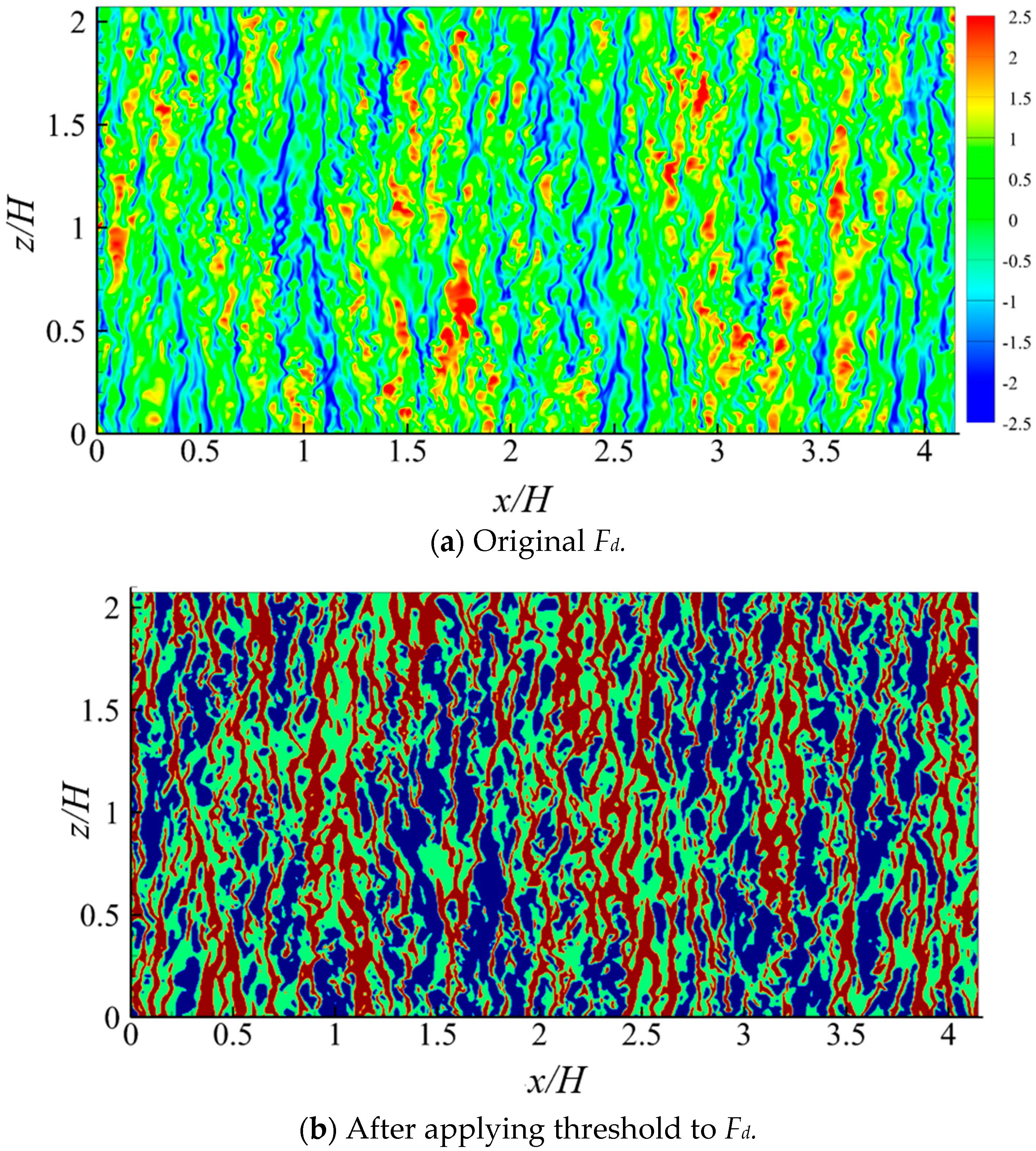
Figure 2a shows the contours of Fd for low-speed streaks at y+ = 21.05. The positive and negative values of Fd indicate the existence of instantaneous streamline fluctuations, forming the low- and high-speed streaks. Low-speed regions (brown), high-speed regions (blue), and other flow regions (green) can be recognized by applying a threshold value of Ct(y+) to the contour map, as shown in Figure 2b.
2.2.2. Image Processing
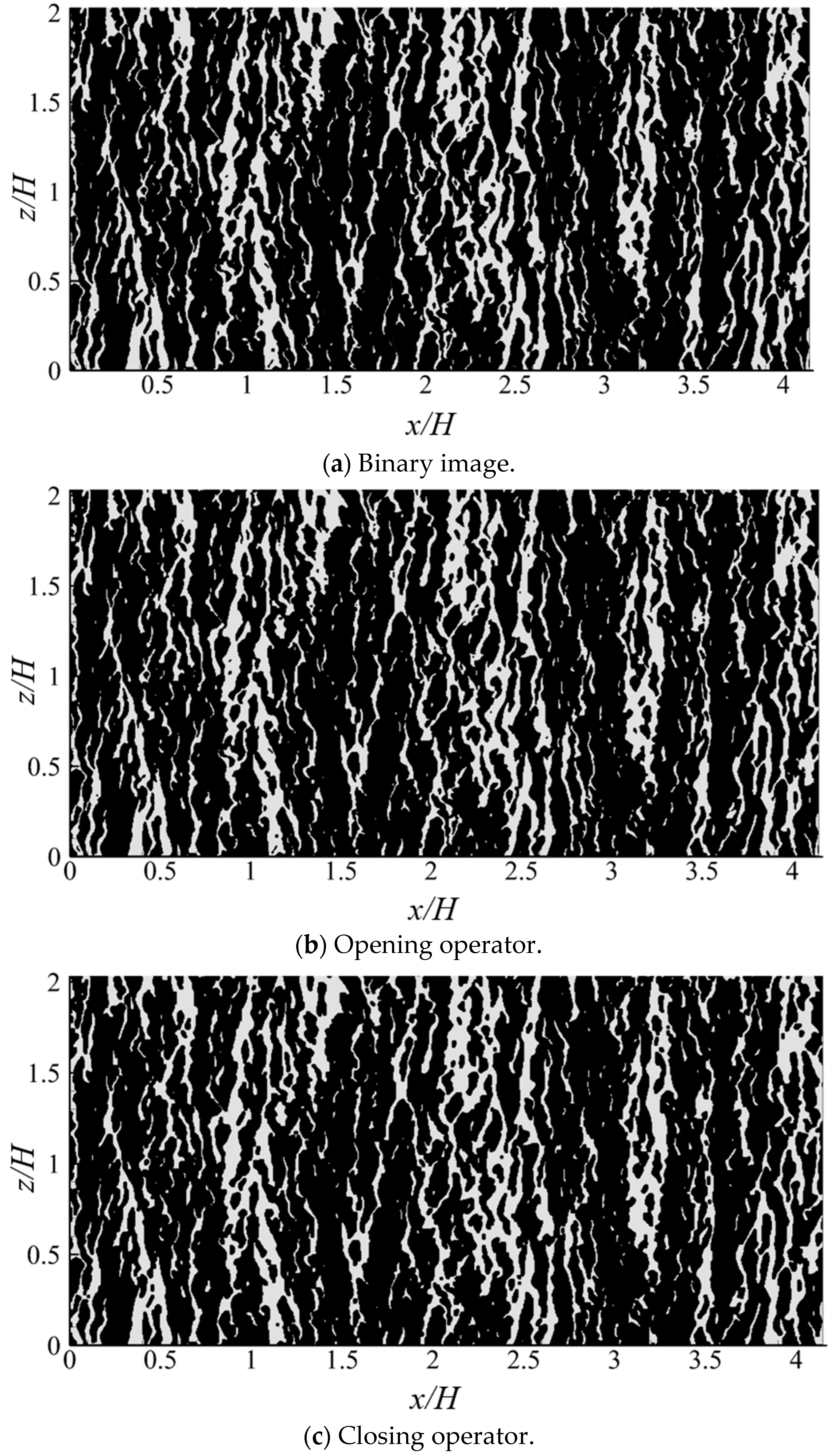
To better quantitatively analyze the low- and high-speed streaks, a binary procedure was used to extract the streaks: values less than −Ct were assigned the value 1, whereas values greater than –Ct were assigned a value 0. Figure 3 shows the image processing procedure for extracting low-speed streaks. The procedure for extracting high-speed streaks is similar, but uses a different Ct threshold value.
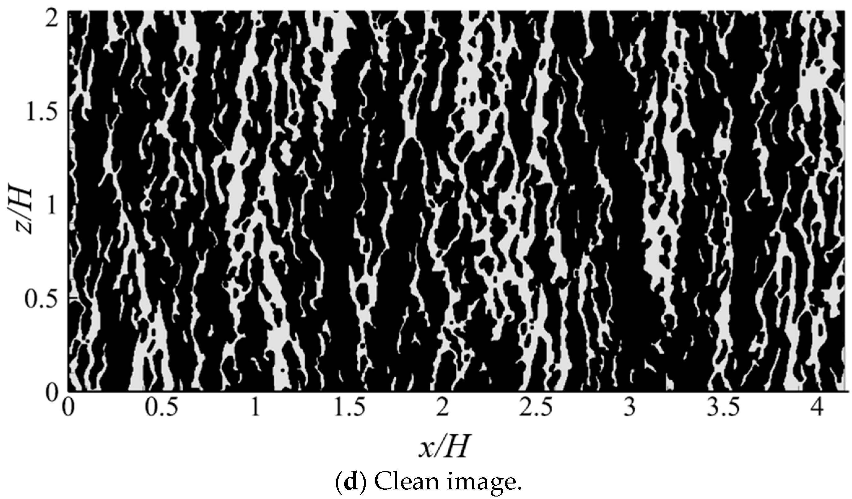
The original Fd image was binarized (Figure 3a), and a basic morphological transformation was used to filter out noise in the binary images. This transformation was done in two steps [23]. First, the opening operator (Figure 3b) and closing operator (Figure 3c) were used to delete some isolated regions and fill some holes. The opening operator is derived from the fundamental morphological operations of dilation as well as erosion and was used to break the adhesion between objects and remove small particle noise; the closing operator combines the operations of erosion and dilation and can be used to connect neighboring regions and fill in small holes. The area of the streak graph does not change significantly during calculation when using the opening and closing operators.
2.2.3. Model of Streaky Structures
We used streak width (w) and the distance between adjacent streaks (d) to scale and characterize streaky structures. As the structures vary spatiotemporally, the image was parsed line-by-line to quantify both w and d. We assumed that the number of streaky structures in a line of the image was ns. The streak widths are denoted by w1, …, wi−1, wi, wi+1, …, wns when the streak distances are denoted by d1, …, di−1, di, di+1, …, dns−1.
For the random row in the image (rth line), the mean streak width of the rth line, w(r), and the mean streak width of the whole velocity field at each y+, W (y+), were obtained by Equations (3) and (4):
where m is the total number of rows of the flow field. Similarly, the mean spanwise distance of each row, d(r), and the mean spanwise distance of the whole velocity field at each y+, D(y+), were calculated by
The dimensionless characteristic scales of the streaks can be obtained by D+ = Du*/v and W+ = Wu*/v. The 30 instantaneous x–z velocity fields (DNS data) were captured at each y position in all cases.
Comparisons between characteristic scales and previous data are given in Figure 8 of Wang et al. [10]. The variations in the mean spanwise distance relative to calculated wall distance are completely feasible, and the above method can be used to analyze the characteristic scales of streaky structures.
3. Results
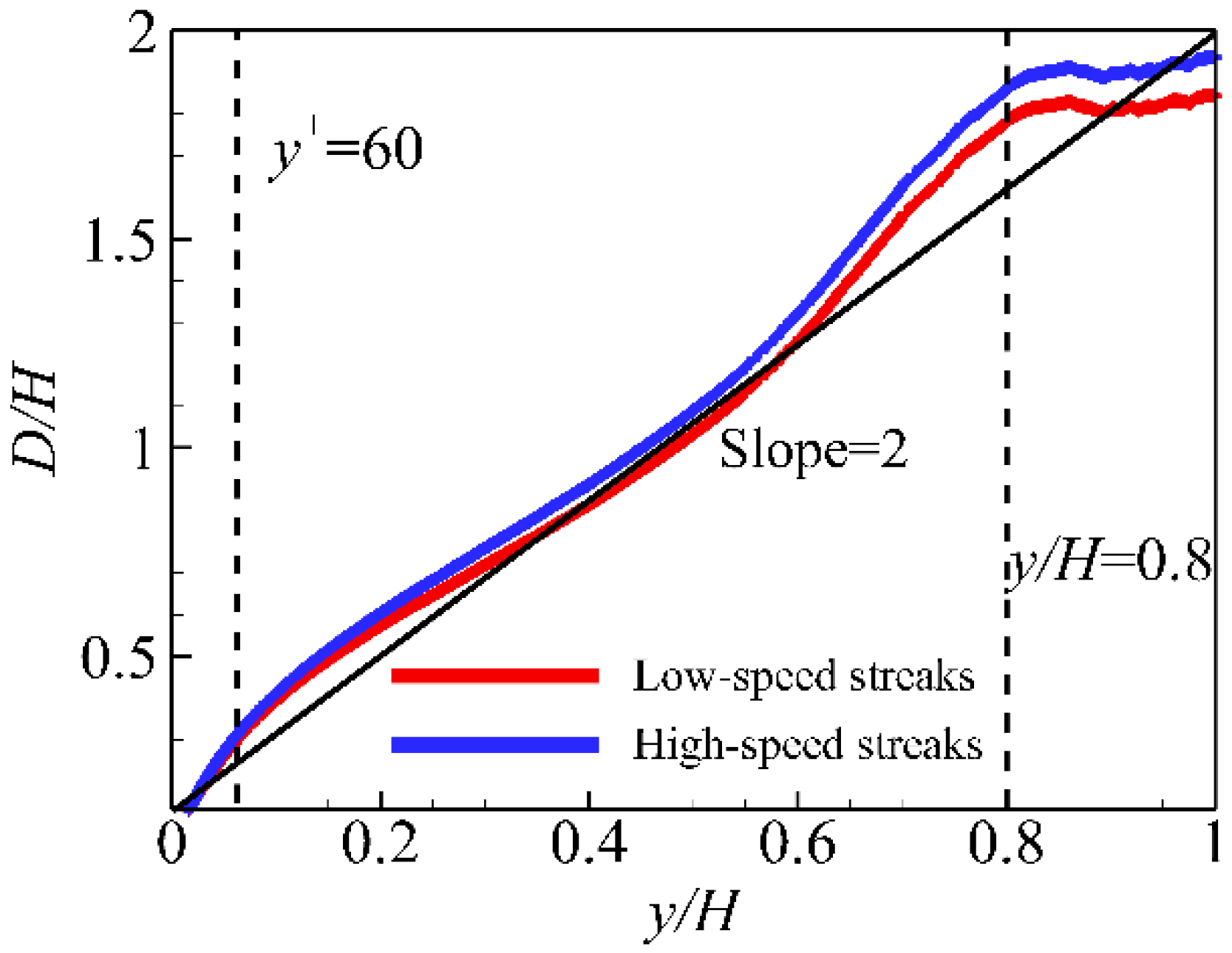
The relationship between the spanwise distance between streaks and the vortex model used is significant for analysis of the entire phenomenon. The spanwise interstreak distances for both low- and high-speed streaks D/H and water depth y/H were plotted. Figure 4 shows that the trend of high-speed streaks is similar to that of low-speed streaks. As water depth y/H increases, D/H reaches a turning point close to half the water depth of the closed-channel flow. The increased amplitude decreases significantly near the half water depth due to a weak boundary layer.
Most research on streaky structures has been concerned with the inner region (y+) and outer region (H) scales. The relationship between two streaky structures of different scales is unclear. We calculated the spanwise distances over the entire water depth continuously for both the inner and outer regions. The results show that the development of streaky structures along the entire flow depth is a continuous process.
D/H increases linearly with y/H in the outer layer (i.e., when 0.1 < y/H < 0.8), and the slope is approximately 2. Streaky structures are closely linked to the vortex model used. Our results are interpreted in the context of the streamwise and attached eddy vortex models as follows.
3.1. Streamwise Vortex Model
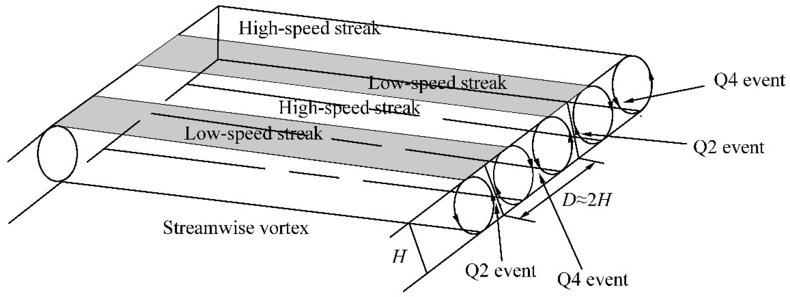
The spanwise distances are approximately twice the water depth, and the formation of streaky structures in the outer layer is related only to water depth. This is consistent with streamwise vortex structures being generated automatically from the self-organization of wall-bound turbulence [7]. In this case, the streamwise vortex also shows that the strong pumping action of low-speed fluid creates an ejection event in the associated second quadrant, Q2 (u < 0, v > 0). Fluid moving at high speed from the water surface toward the bed creates a sweep event in Q4 (v < 0, u > 0). The low- and high-speed streaks are located at the downwelling and upwelling sides of the streamwise vortices respectively.
3.2. Attached Eddy Vortex Model
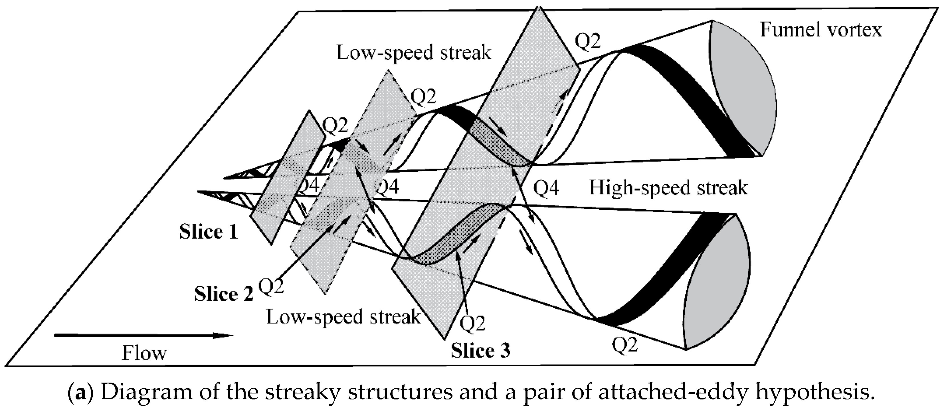
Figure 6a shows that the increases in the characteristic scales of the streaks are linear, which is a core assumption of Townsend’s attached eddy vortex hypothesis [17,23]. Our results indicate the suitability of the attached eddy vortex model.
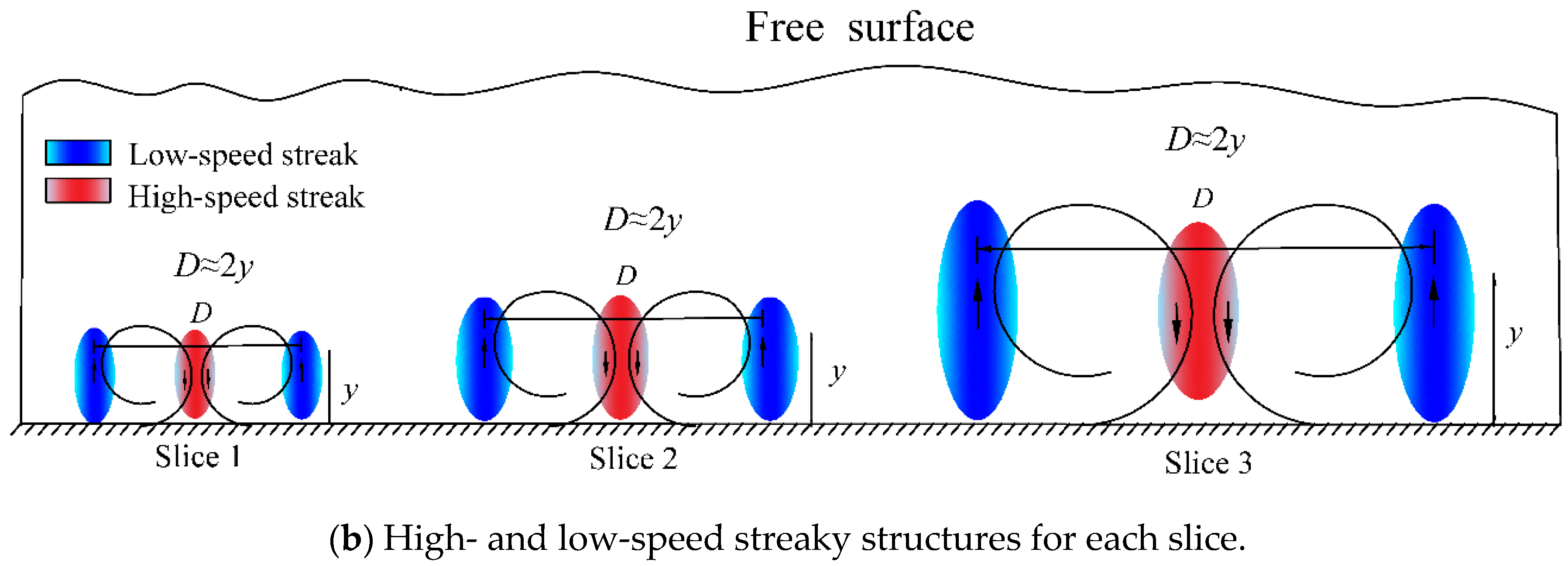
Figure 6a shows that, according to the model, the attached eddy vortex develops from the near-wall region into a conical vortex in the streamflow direction. The formation mechanics of low- and high-speed streaks and the Q2/Q4 events are similar to those of the streamwise vortex. In particular, the spanwise distances between adjacent low-speed (or high-speed) streaks are closely related to the size of the streamwise vortices and thus linearly proportional to y. Three cross-stream plane sections (slices) of the attached eddies at different water depths y are shown in Figure 6; the blue and red backgrounds indicate the low-speed and high-speed streaks, respectively. Figure 6a shows the Q2\Q4 events when Figure 6b shows that the dimensions of the vortex increase linearly as water depth increases and the relationship between D and h remains basically constant with D ≈ 2h. Overall, the attached eddy vortex model explains the distance between adjacent streaks from the inner region to the outer region.
3.3. Hairpin Vortex Model
The hairpin vortex model developed by Adrian is a relatively new vortex model [24]. We investigated the positional relationships between spanwise vortices and streaky structures in the x–z plane to determine the suitability of the hairpin vortex model.
3.3.1. Vortex Extraction in the X–Z Plane
We used the two-dimensional swirling-strength λci-criterion [25]. Streaky structures form in the in x–z plane, so a brief introduction to extracting a vortex in the x–z plane is given.
The swirling strength λci is given by
where
Following Wu and Christensen [26], we defined the normalized swirling strength Λci as , where ωz is the fluctuating spanwise vorticity and λci and Λci are swirling strength discriminators. is the local root mean square of Λci at the wall-normal position y, and we defined the normalized swirling strength Ωci by
In an ideal fluid, there is a clear boundary between rotating and irrotational fluid. Zero (0) can be used as a threshold to easily extract the vortex. However, in a nonideal (actual) fluid, viscosity causes dissipation of the vortex, which greatly complicates vortex identification. We used a non-zero threshold of 1.5 to identify a vortex, following the recommendation of Wu and Christensen [26], so that
Negative or positive values of Ωci in Equation (8) represent a clockwise or counterclockwise vortex, respectively.
3.3.2. Vortex Density
When the vortex structure has been determined by the preceding methods, the vortex population density Π+ is calculated by
where Nvortex is the spanwise number of vortices at position y+.
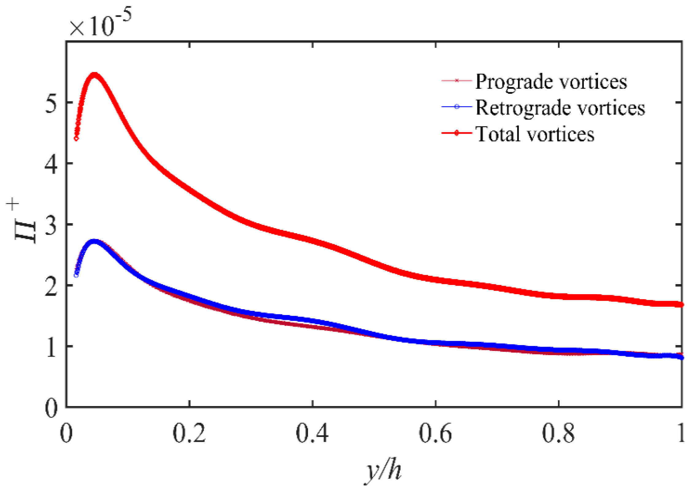
The prograde and retrograde vortices in the x–z plane were separated, and the population densities of the vortices were computed for each position of y+. Figure 7 shows that the population density of 2D vortices varies with water depth, reaching a maximum in the near-wall region at y+ = 40.22. This result may be partly due to the number of streamwise vortices in the deeper water. In the outer region, vortex density decreases gradually as y+ increases. As the shear stress in the x–z plane is approximately zero, the population density of prograde vortices is equal to that of retrograde vortices at each y+ position. These results agree with those obtained by Chen et al. [27], which confirms the logic of our vortex extraction method.
3.3.3. Location of Vortices and Streaks
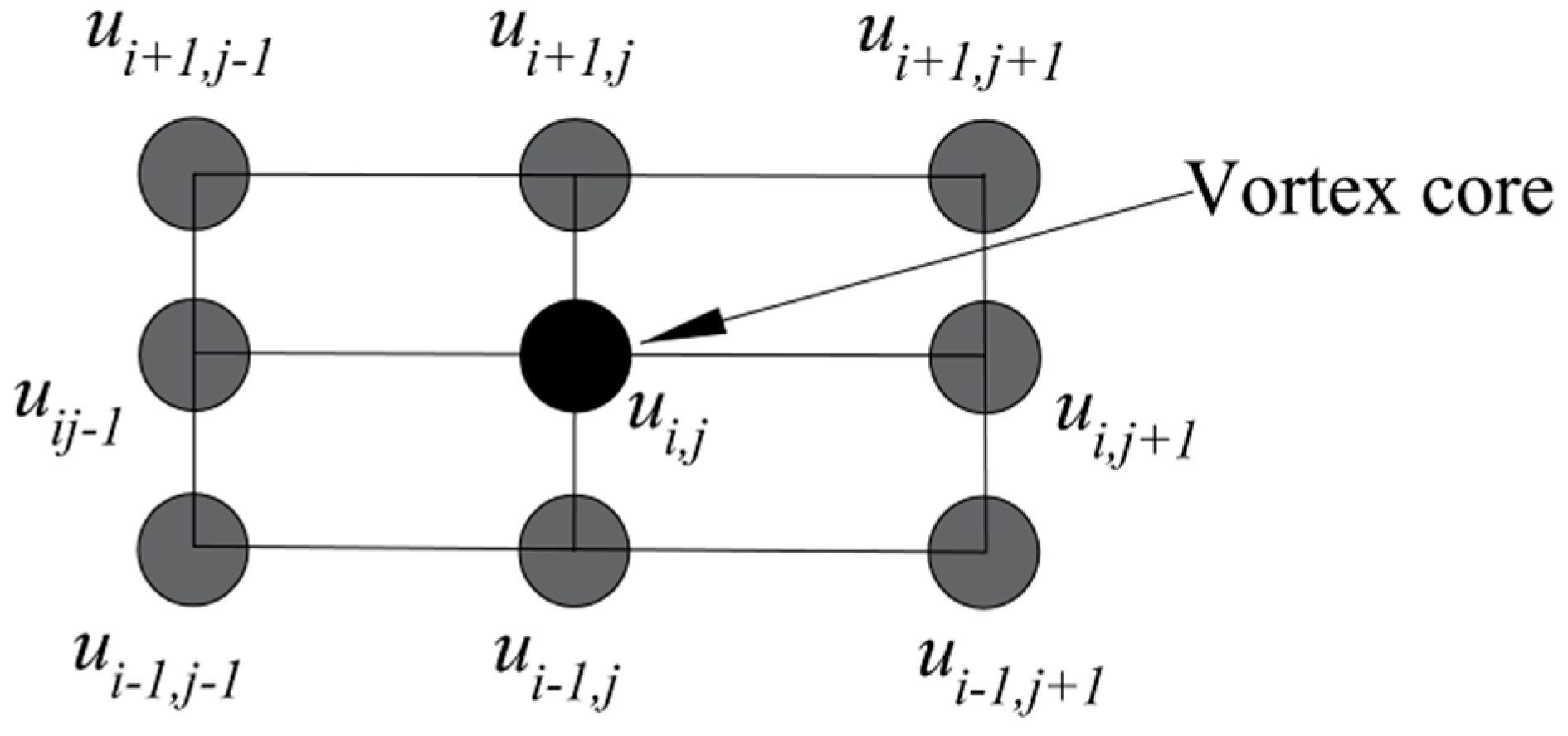
Figure 8 shows the cores of spanwise vortices surrounded by nine velocity vectors (red), high-speed streaks (yellow), low-speed streaks (blue), and the in-between region (green) that were obtained by the preceding methods. We extracted and analyzed 400 × 800 grid points in the x–z plane. The dimensionless area is 3040 × 3040, and x+ and z+ represent the dimensionless length along the streamwise and spanwise directions, respectively.
To further investigate the relationship between streaky structures and spanwise vortices, the vortex core (ui,j) velocity and the eight surrounding streamwise velocities (Figure 9) were averaged using Equation (10). Equation (11) was then used to calculate Fd at the core of each vortex. We use Ct(y) to identify the region of the distribution of vortex cores.
where ū is the average velocity of spanwise vortices in the x–z plane, ū′ is the fluctuating velocity, and is the detection function of average vortex velocity. We can now calculate the statistical measures of the vortices in different streaky structures.
In previous research, streaks have generally been divided into low- and high-speed. However, to obtain a more detailed analysis of the relationships between spanwise vortices and streaky structures, we divided the x–z plane into three types using the threshold Ct(y+): low-speed streaks, high-speed streaks, and in-between regions.
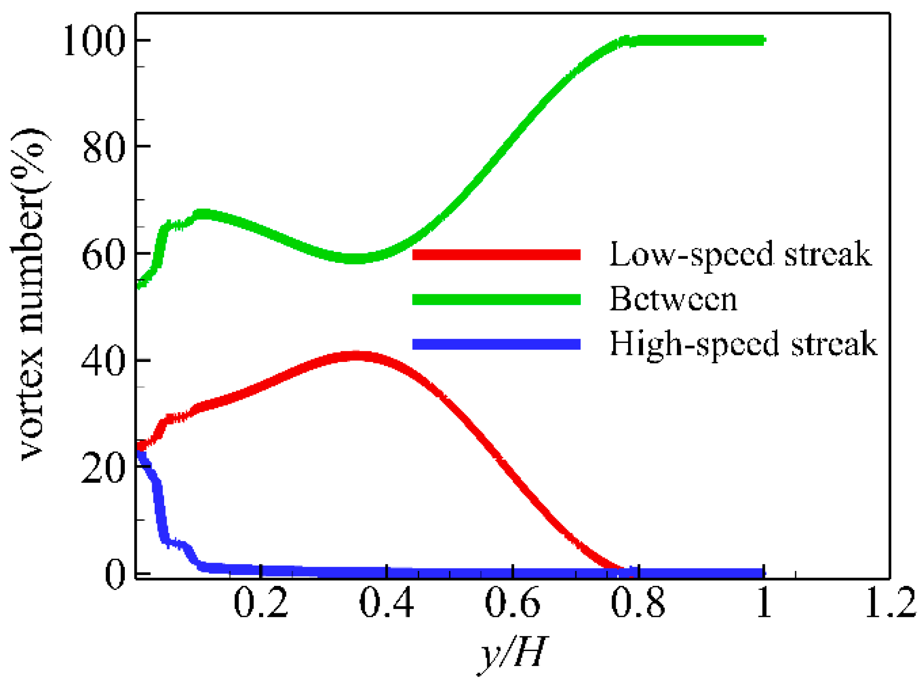
Figure 10 shows that the numbers of vortices differ greatly within the different streaks. The spanwise vortices in the in-between region occur in the greatest numbers, followed by low-speed streaks, with the least numbers in the high-speed streaks. When y/H > 0.1 the number of vortices in high-speed streaks is approximately equal to 0.
It should be noted that the three areas occupied by the three types are also different. By dividing the number of vortices by the area containing them, we eliminated the influence of area from our analysis to better understand the distributions of spanwise vortices located in streaky structures.
3.3.4. Vortex Density in Different Streaks
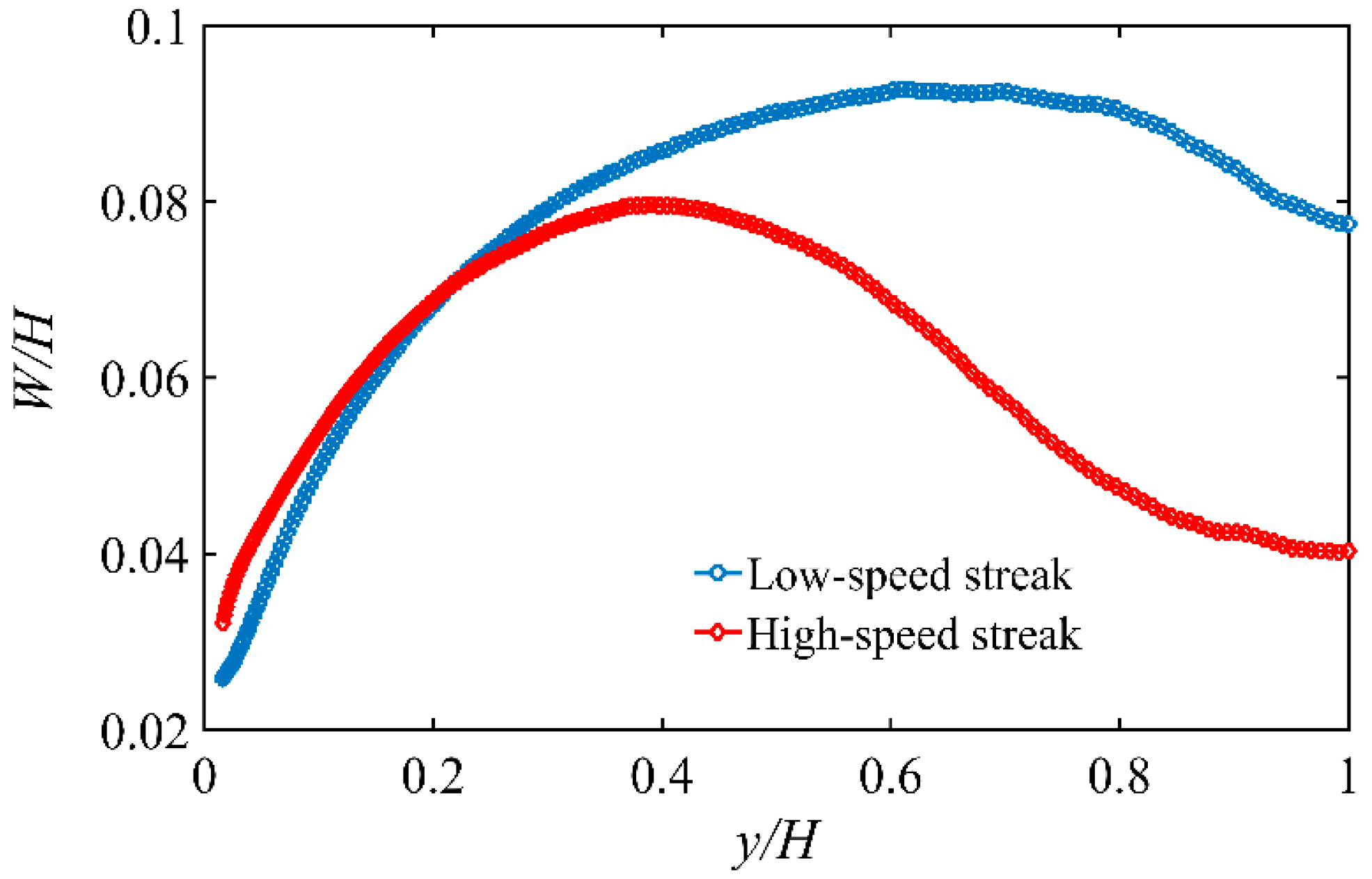
We first calculated the areas of the low- and high-speed streaks. The values of both low- and high-speed streak widths are influenced by the threshold value (Ct) and are difficult to recognize relative to the spanwise distance. If Ct is too large, the streak width will not include the whole with of the streak; nevertheless, if Ct is too small, the streak width will contain parts of the in-between region. However, even with different threshold values, the change tendencies are basically consistent. Here, we used the threshold value suggested by Lin et al. [6] to identify the width of low- and high-speed streaks. Figure 11 shows that as y+ increases, streak width first increases and then decreases. As the water depth increases from inner region to outer region, the streak scale also increases. When water depth is close to the surface (about 0.7H), the weak boundary layer restrains the streak scale, and the streak width will decrease. This trend is stable and clearly demonstrated.
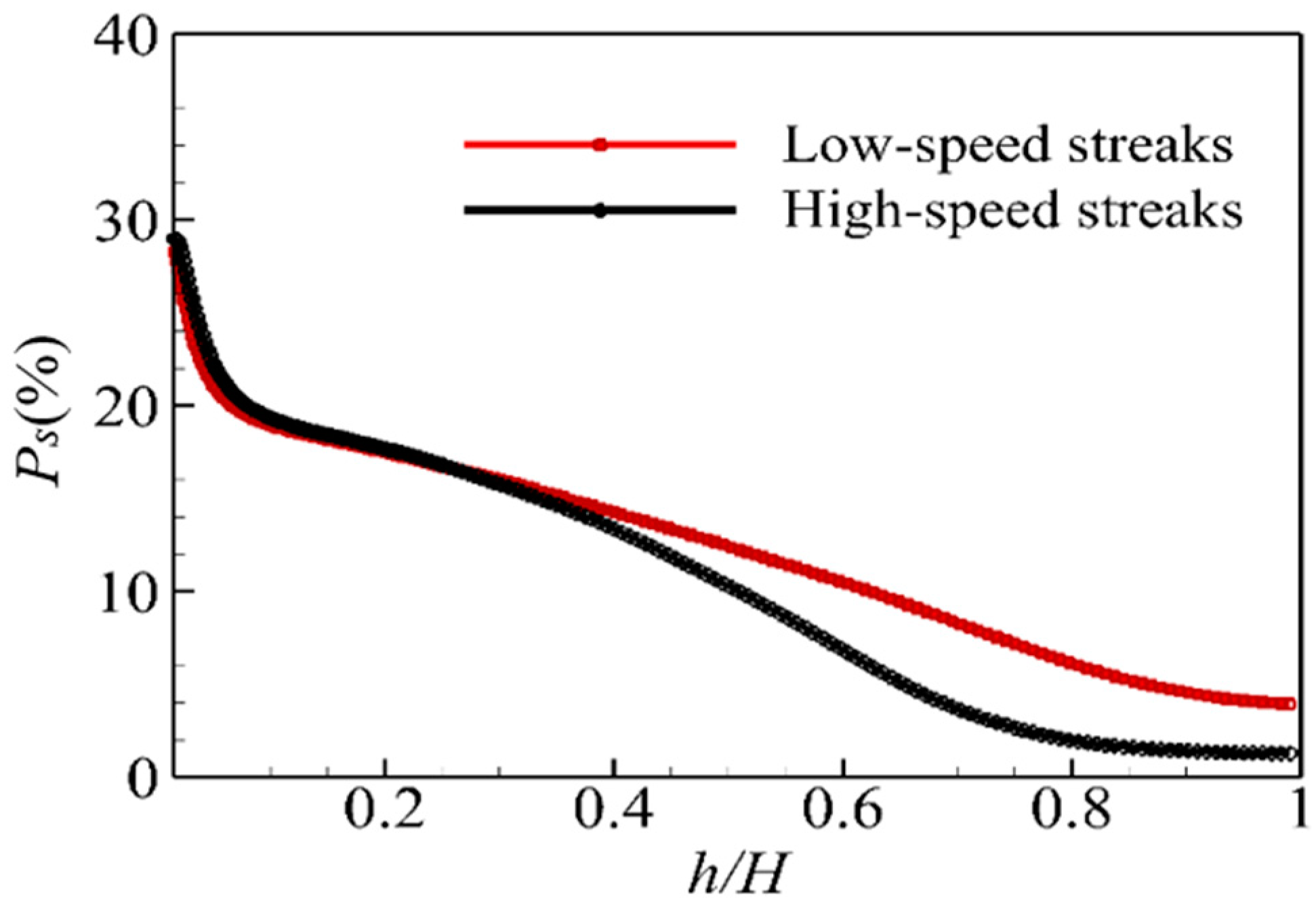
The area percentages of low- and high-speed streaks in the x–z plane at each position y+ are also important characteristic dimensions and can be regarded as the normalized areas of streaks. The area percentage, defined as Ps, can be obtained by
where As is the total area of low- or high-speed streaks and At is the total area of the flow field (2048 × 1536). Figure 12 shows that the percentage area of both low- and high-speed streaks decreases as y+ increases. In the near-wall region (y/h < 0.1), the gradients are steep; in the outer region (y/h > 0.3), the decreasing trends become less steep. This result shows that the streaks occur mainly in the near-wall region where there is high shear stress. Mean shear stress decreases as y/h increases, and so does its effect on the streaks. Streaks in the outer region decrease in number and so the percentages of both low- and high-speed streaks in the x–z plane also decrease.
3.3.5. Calculation of Vortex Density
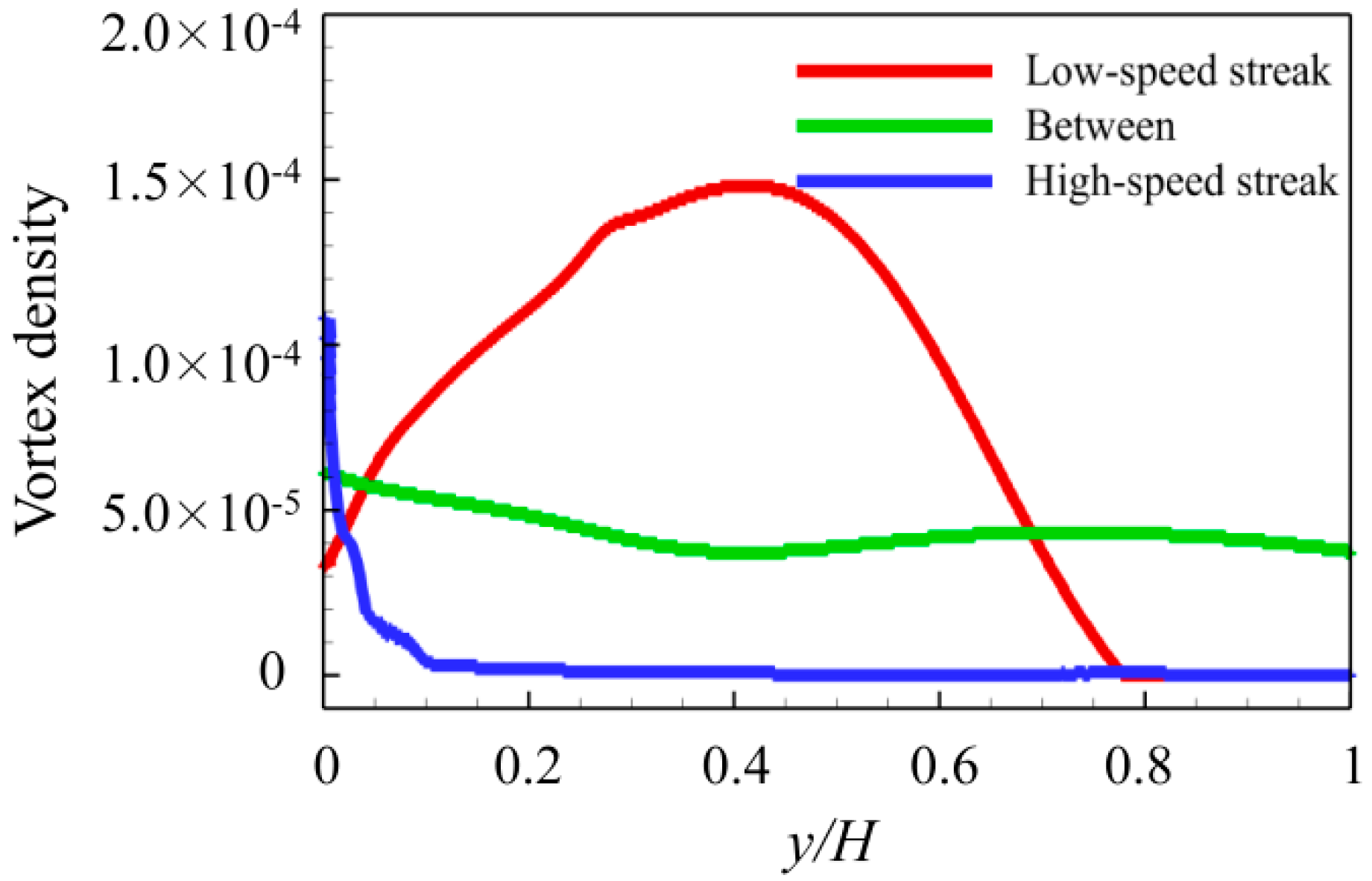
Equation (10) was used to calculate the density of spanwise vortices in different streaky structures, as shown in Figure 13. The density of spanwise vortices is highest in low-speed streaks, intermediate in the in-between region and least in the high-speed streaks. Thus, there are big differences between the number of vortices and vortex density located in different streaky structures.
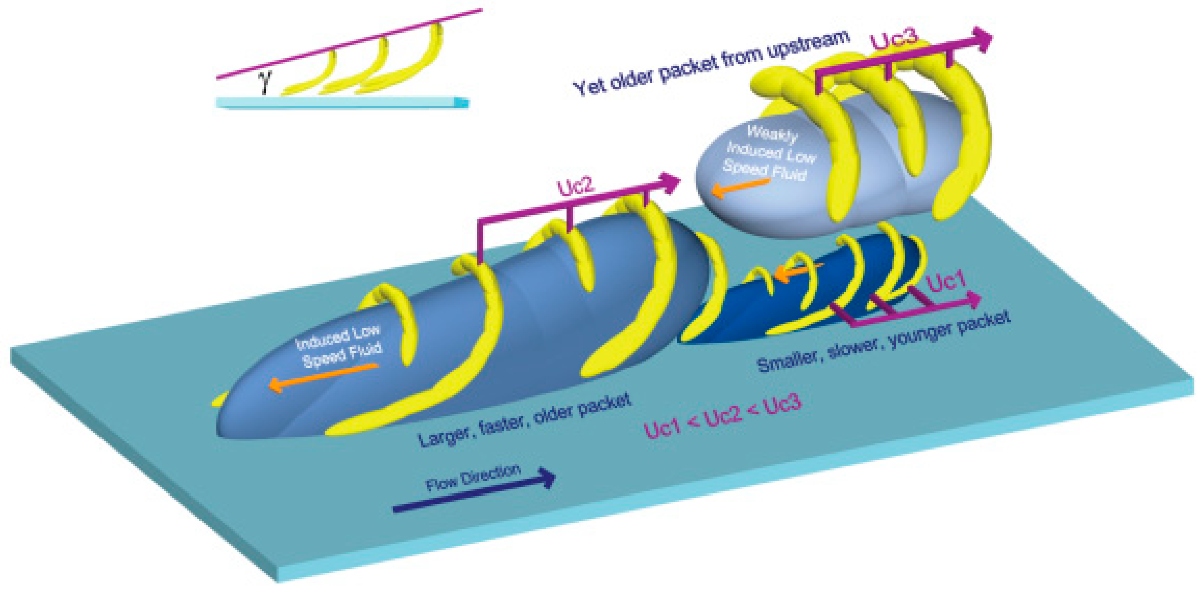
The hairpin vortex model developed by Adrian [24] has gained widespread acceptance, due to experimental visualization using particle image velocimetry and direct numerical simulation. Figure 14 shows the standard coherent structure model of a hairpin vortex developed by Adrian [24]. The alignment of coherent vortices induces a low-speed fluid region inside the hairpin packets. Due to the closed-loop feedback cycle between hairpin vortex cells and streamwise vortices [1,28], the streamwise vortices are stable.
Research into hairpin vortex behavior has become an important direction of research. However, the sample sizes used in the research are fairly small, so the regularity of the relationship between streaky structures and spanwise vortices in the x–z plane must be further researched by analyzing large samples.
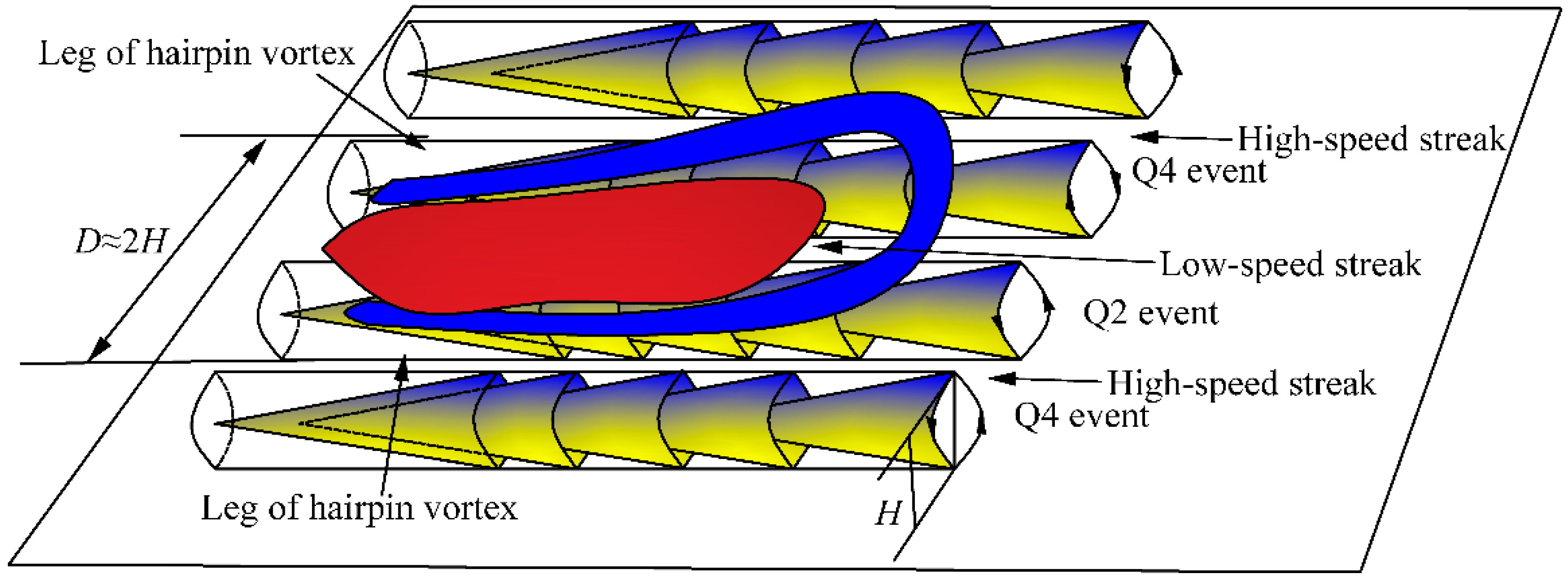
We obtained statistics from large DNS data samples, and we found that spanwise vortex density in low-speed streaks is greater than in high-speed streaks. This result indicates that hairpin vortex legs are closer to the low-speed streaks and further from the high-speed streaks. Thus, the results we obtained exhibit an important feature of hairpin vortex legs when they envelop low-speed streaks to move along the quasi-streamwise direction, as shown in Figure 14. The legs of the hairpin vortex are spanwise vortices in the x–z plane, as shown in Figure 15. Spanwise vortices are mainly distributed in the region of low-speed streaks, consistent with the structure of hairpin vortices. Our results support the logic of the hairpin vortex model and reveal mechanisms of hairpin vortex behavior more explicitly.
4. Discussion and Conclusions
4.1. Discussion
A large-scale vortex is a conceptual model, or representation, of a natural phenomenon intended to be used in the provision of logical explanations of all kinds of coherent structures in turbulent fluids. Classical and prevailing views of vortices have led to many vortex models being developed. We identified both low- and high-speed streaks from the wall to the surface using image processing technology; the meandering large scale motions are impossible to ignore. The low- and high-speed streaks are formed by an ejection event (Q2, u < 0, v > 0) and a sweep event (Q4, v < 0, u > 0) [14,18]. We used the super-streamwise vortex (Figure 5) as the interpretative model to explain the preceding results and the spanwise distance of nearby streaks (2H). We found that the scale of the streaks increased in proportion to their distance from the wall. The result is consistent with the classical model, which combines length growth with growth in eddies, developed by Townsend [17]. Our results also explain the logarithmic growth in open channel flow. The distributions of spanwise vortex density in low- and high-speed streaky structures suggest further research into hairpin vortices. We statistically sampled large datasets to compare and analyze three vortex models. Our analysis of the results shows the benefit of explaining coherent structures from the three different model perspectives.
The literature contains little record of large dataset statistical sampling, but it is urgently needed to demonstrate the suitability of different vortex models and to clarify the relationships between them. As stated in the introduction, the large-scale streamwise vortex model provides a good explanation of the coherent structures of Q2/Q4 events and the spanwise distances between adjacent streaky structures near the water surface (which is about 2H). However, the large-scale streamwise vortex model is relatively coarse and represents a large structure (Figure 5), and it cannot accurately explain the continuous development of streaks from the inner region to the outer region. The attached eddy vortex model cannot provide a precise organized structure for the large vortices that accumulate in turbulence. The hairpin vortex model requires more usage and analysis to show its suitability.
Vortex models are limited. However, our research into the characteristic dimensions of streaky structures across the entire water depth, described in this study, leads us to conclude: the streamwise vortex model, the attached eddy vortex model, and the hairpin vortex model are all suitable models in certain circumstances.
We used quantitative analysis to develop a theoretical model in which packets of attached eddy vortices self-organize and accumulate along the flow direction, thereby forming a cumulative vortex structure, the streamwise vortex. Figure 16 shows that many attached eddy vortices are connected along the flow direction to form the large-scale structure of a streamwise vortex. This behavior provides more details about the formation of large-scale streamwise vortexes. The model explains the characteristics of streamwise vortices (Q2/Q4 events and low- and high-speed streaky structures) and linear streaks based on water depth. Our investigation into the spatial relationships between spanwise vortex density and streaky structures shows that the legs of the hairpin vortex model envelop low-speed streaks. These low-speed hairpin vortex legs can be organized and accumulated into larger-scale quasi-streamwise vortices (Figure 16).
Further analysis of the details of the vortex models led us to propose a simple hypothesis: the three coherent structures, modeled individually as a streamwise vortex, while an attached eddy vortex and a hairpin vortex both exist separately in turbulent flow. It is likely that they are all manifestations of the same turbulent structure under different paradigmatic approaches, as shown in Figure 16.
4.2. Conclusions
We based this study on 30 sets of closed-channel flow DNS data. Image processing was employed to identify low- and high-speed streaks, using a detection function and a threshold value, Ct. Statistical methods were used to calculate the characteristic dimensions of both low- and high-speed streaks. We investigated three models of coherent structures (streamwise vortex, attached eddy vortex, and hairpin vortices) and demonstrated their application. Analysis of the characteristic dimensions of streaky structures and vortices and further analysis of the relationships among the three vortex models led us to suggest a straightforward hypothesis. The results we obtained are summarized as follows.
- (1)
- The average width of streaks and the average distance between adjacent streaks that we observed are consistent with the results of previous studies, which indicates the suitability of our method of identifying and calculating both low- and high-speed streaky structures.
- (2)
- The development of streaks from the inner turbulent region to the outer region is a continuous process. The length of streaky structures increases linearly with the water depth, and it is approximately twice the water depth. This result also shows the suitability of both the streamwise vortex and the funnel vortex models.
- (3)
- The spanwise vortex density in the x–z plane is greatest within low-speed streaks, intermediate in the in-between region, and least in the high-speed streaks. We infer that the legs of the hairpin vortices envelop the low-speed streaky structures to move in the streamwise direction and conclude that the hairpin vortex model provides a suitable representation.
- (4)
- The theoretical model of the locations in the x–z plane of streamwise vortices, attached-eddy vortices and hairpin vortices established the possibility of the coexistence of three vortex structures; this recognition increases our understanding of the mechanics of coherent structures in turbulent flows.
Author Contributions
H.W. performed the data collection, data processing, and manuscript preparation; G.P. assisted with the data analysis. All authors participated in the revision of the manuscript and graphics.
Funding
The study is financially supported by the National Natural Science Foundation of China (Grant No. 51709047), the CRSRI Open Research Program (Grant No. CKWV2018461/KY), and the Open Research Fund of State Key Laboratory of Simulation and Regulation of Water Cycle in River Basin (China institute of Water Resources and Hydropower Research, Grant No. IWHR-SKL-KF201815).
Conflicts of Interest
The authors declare no conflicts of interest.
Abbreviations
| Parameter Description Unit | |
| As | Total area of low- or high-speed streaky structures |
| At | Total area of the flow field (2048 × 1536) |
| Ct(y+) | Streak threshold at y+ |
| d(r) | Dimensionless spanwise distance at each y+ |
| D | Nondimensional spanwise distance |
| Detection function value of average vortex velocity | |
| Fd | Dimensionless value of detection function |
| m | Total number of rows of the flow field |
| Nx | Grid numbers in the x direction |
| Ny | Grid numbers in the y direction |
| Nz | Grid numbers in the x direction |
| Nvortex | Number of spanwise vortices at position y+ |
| Ps | Area percentages of low- and high-speed streaky structures |
| u | Instantaneous velocity in the x direction m/s |
| u* | Friction velocity m/s |
| uij | Velocity at the position of vortex core |
| ū | Average velocity of spanwise vortices in the x–z plane m/s |
| ū′ | Fluctuating velocity m/s |
| u′ | Streamwise velocity fluctuation m/s |
| v | Instantaneous velocity in the y direction m/s |
| w | Instantaneous velocity in the z direction m/s |
| W | Average nondimensional width |
| x | Streamwise direction |
| Δx | Grid resolution in the x directions |
| y* | Inner scale |
| y | Vertical direction |
| Δyc | Wall-normal grid spacing at the channel left |
| z | Spanwise direction |
| Δz | Grid resolution in the z directions |
| (m, n) | Grid position in the x–z plane |
| ustd(y+) | Standard deviation of the streamwise velocity at y+ |
| λci | Two-dimensional swirling-strength 1/s |
| Λci | Dimensionless swirling strength |
| ωz | Fluctuating spanwise vorticity 1/s |
| Local root mean square of Λci at the wall-normal position y | |
| Ωci | Normalized swirling strength |
| Π+ | Vortex population density |
| υ | Kinematic viscosity cm2/s |
References
- Zhong, Q.; Chen, Q.G.; Wang, H.; Li, D.X.; Wang, X.K. Statistical analysis of turbulent super-streamwise vortices based on observations of streaky structures near the free surface in the smooth open channel flow. Water Resour. Res. 2016, 52, 3563–3578. [Google Scholar] [CrossRef] [Green Version]
- Kline, S.J.; Reynolds, W.C.; Schraub, F.A.; Runstadler, P.W. The structure of turbulent boundary layers. J. Fluid Mech. 1967, 30, 741–773. [Google Scholar] [CrossRef] [Green Version]
- Kähler, C.J. Investigation of the spatio-temporal flow structure in the buffer region of a turbulent boundary layer by means of multiplane stereo PIV. Exp. Fluids 2004, 36, 114–130. [Google Scholar] [CrossRef]
- Carlier, J.; Stanislas, M. Experimental study of eddy structures in a turbulent boundary layer using particle image velocimetry. J. Fluid Mech. 2005, 535, 143–188. [Google Scholar] [CrossRef]
- Lagraa, B.; Labraga, L.; Mazouz, A. Characterization of low-speed streaks in the near-wall region of a turbulent boundary layer. Eur. J. Mech. B Fluids 2004, 23, 587–599. [Google Scholar] [CrossRef]
- Lin, J.; Laval, J.; Foucaut, J.; Stanislas, M. Quantitative characterization of coherent structures in the buffer layer of near-wall turbulence. Exp. Fluids 2008, 45, 999–1013. [Google Scholar] [CrossRef]
- Nakagawa, H.; Nezu, I. Structure of space-time correlations of bursting phenomena in an open-channel flow. J. Fluid Mech. 1981, 104, 1–43. [Google Scholar] [CrossRef]
- Shvidchenko, A.B.; Pender, G. Macroturbulent structure of open-channel flow over gravel beds. Water Resour. Res. 2001, 37, 709–719. [Google Scholar] [CrossRef]
- Roy, A.G.; Buffin-Belanger, T.; Lamarre, H.; Kirkbride, A.D. Size, shape and dynamics of large-scale turbulent flow structures in a gravel-bed river. J. Fluid Mech. 2004, 500, 1–27. [Google Scholar] [CrossRef] [Green Version]
- Wang, H.; Zhong, Q.; Wang, X.K.; Li, D.X. Quantitative characterization of streaky structures in open-channel flows. J. Hydraul. Eng. 2017, 143, 04017040. [Google Scholar] [CrossRef]
- Sukhodolov, A.N.; Nikora, V.I.; Katolikov, V.M. Flow dynamics in alluvial channels: The legacy of Kirill V. Grishanin. J. Hydraul. Res. 2011, 49, 285–292. [Google Scholar] [CrossRef]
- Fox, J.F.; Patrick, A. Large-scale eddies measured with large scale particle image velocimetry. Flow Meas. Instrum. 2008, 19, 283–291. [Google Scholar] [CrossRef]
- Panton, R.L. Overview of the self-sustaining mechanisms of wall turbulence. Prog. Aerosp. Sci. 2001, 37, 341–383. [Google Scholar] [CrossRef]
- Gulliver, J.S.; Halverson, M.J. Measurements of large streamwise vortices in an open-channel flow. Water Resour. Res. 1987, 23, 115–123. [Google Scholar] [CrossRef]
- Imamoto, H.; Ishigaki, T. Visualization of longitudinal eddies in an open channel flow. In Proceedings of the Fourth International Symposium on Flow Visualization IV, Paris, France, 26–29 August 1986; pp. 323–337. [Google Scholar]
- Rashidi, M.; Banerjee, S. Turbulence structure in free-surface channel flows. Phys. Fluids 1988, 31, 2491–2503. [Google Scholar] [CrossRef]
- Townsend, A.A. Equilibrium layers and wall turbulence. J. Fluid Mech. 1961, 11, 97–120. [Google Scholar] [CrossRef]
- Adrian, R.J.; Marusic, I. Coherent structures in flow over hydraulic engineering surfaces. J. Hydraul. Res. 2012, 50, 451–464. [Google Scholar] [CrossRef]
- Nezu, I.; Rodi, W. Open-channel flow measurements with a laser Doppler anemometer. J. Hydraul. Eng. 1986, 112, 335–355. [Google Scholar] [CrossRef]
- Nezu, I.; Nakagawa, H.; Jirka, G.H. Turbulence in open-channel flows. J. Hydraul. Eng. 1994, 120, 1235–1237. [Google Scholar] [CrossRef]
- Del Alamo, J.C.; Jiménez, J.; Zandonade, P.; Moser, R.D. Scaling of the energy spectra of turbulent channels. J. Fluid Mech. 2004, 500, 135–144. [Google Scholar] [CrossRef] [Green Version]
- Herpin, S.; Stanislas, M.; Soria, J. The organization of near- wall turbulence: A comparison between boundary layer SPIV data and channel flow DNS data. J. Turbul. 2010, 11, 1–30. [Google Scholar] [CrossRef]
- Kaftori, D.; Hetsroni, G.; Banerjee, S. Particle behavior in the turbulent boundary layer. I. Motion, deposition, and entrainment. Phys. Fluids 1995, 7, 1095–1106. [Google Scholar] [CrossRef]
- Adrian, R.J. Hairpin vortex organization in wall turbulence. Phys. Fluids 2007, 19, 041301. [Google Scholar] [CrossRef] [Green Version]
- Zhou, J.; Adrian, R.J.; Balachandar, S.S.; Kendall, T.M. Mechanisms for generating coherent packets of hairpin vortices in channel flow. J. Fluid Mech. 1999, 387, 353–396. [Google Scholar] [CrossRef]
- Wu, Y.; Christensen, K.T. Population trends of spanwise vortices in wall turbulence. J. Fluid Mech. 2006, 568, 55–76. [Google Scholar] [CrossRef] [Green Version]
- Chen, H.; Adrian, R.J.; Zhong, Q.; Wang, X.K. Analytic solutions for three dimensional swirling strength in compressible and incompressible flows. Phys. Fluids 2014, 26, 81701. [Google Scholar] [CrossRef]
- Zhong, Q.; Li, D.X.; Chen, Q.G.; Wang, X.K. Coherent structures and their interactions in smooth open channel flows. Environ. Fluid Mech. 2015, 15, 653–672. [Google Scholar] [CrossRef]
Figure 1.
The computation region of direct numerical simulation (DNS) in closed channel flow.

Figure 2.
Visualization of streaks represented by the dimensionless value of detection function Fd: (a) original Fd with the range of the color bar set from −2.5 to 2.5; (b) after applying the threshold value to Fd.
Figure 2.
Visualization of streaks represented by the dimensionless value of detection function Fd: (a) original Fd with the range of the color bar set from −2.5 to 2.5; (b) after applying the threshold value to Fd.

Figure 3.
Image processing: (a) binary image, (b) opening operator, (c) closing operator, and (d) clean image.
Figure 3.
Image processing: (a) binary image, (b) opening operator, (c) closing operator, and (d) clean image.


Figure 4.
Spanwise distances of streaks; D/H varies with water depth y/H.

Figure 5.
Representation of the streamwise vortex model.

Figure 6.
Streaky structures described in terms of the attached eddy hypothesis: (a) A pair of vortices and the (b) corresponding high- and low-speed streaky structures for each slice.
Figure 6.
Streaky structures described in terms of the attached eddy hypothesis: (a) A pair of vortices and the (b) corresponding high- and low-speed streaky structures for each slice.


Figure 7.
Vortex population density in the x–z plane.

Figure 8.
Positional distributions of streaks and spanwise vortices.

Figure 9.
Grid for streamwise velocity u showing the core of the vortex.

Figure 10.
Vortex numbers in low- and high-speed streaks and in-between regions.

Figure 11.
Characteristic dimensions (width) of low- and high-speed streaks varying with y+.

Figure 12.
Percentage area of low- and high-speed streaks along the x–z plane.

Figure 13.
Vortex densities located in different streaky areas.

Figure 14.
Representation of hairpins and hairpin packets by Adrian [24].
Figure 14.
Representation of hairpins and hairpin packets by Adrian [24].

Figure 15.
Representation of hairpin vortex and spanwise vortex.

Figure 16.
Theoretical models of a streamwise vortex, an attached eddy vortex, and a hairpin vortex in the x–z plane.
Figure 16.
Theoretical models of a streamwise vortex, an attached eddy vortex, and a hairpin vortex in the x–z plane.


Table 1.
Parameters of the DNS (data from Del Alamo et al. [21]).
Table 1.
Parameters of the DNS (data from Del Alamo et al. [21]).
| Parameter | Lx/H | Lz/H | Ly/H | Δx+ | Δz+ | Δyc+ | Nx | Nz | Ny |
|---|---|---|---|---|---|---|---|---|---|
| Original | 8π | 3π | 2 | 7.6 | 3.8 | 7.6 | 3072 | 2304 | 385 |
| Present study | 16π/3 | 2π | 1 | 7.6 | 3.8 | 7.6 | 2048 | 1536 | 193 |
© 2019 by the authors. Licensee MDPI, Basel, Switzerland. This article is an open access article distributed under the terms and conditions of the Creative Commons Attribution (CC BY) license (http://creativecommons.org/licenses/by/4.0/).
Share and Cite
MDPI and ACS Style
Wang, H.; Peng, G.; Chen, M.; Fan, J. Analysis of the Interconnections between Classic Vortex Models of Coherent Structures Based on DNS Data. Water 2019, 11, 2005. https://doi.org/10.3390/w11102005
AMA Style
Wang H, Peng G, Chen M, Fan J. Analysis of the Interconnections between Classic Vortex Models of Coherent Structures Based on DNS Data. Water. 2019; 11(10):2005. https://doi.org/10.3390/w11102005
Chicago/Turabian StyleWang, Hao, Guoping Peng, Ming Chen, and Jieling Fan. 2019. "Analysis of the Interconnections between Classic Vortex Models of Coherent Structures Based on DNS Data" Water 11, no. 10: 2005. https://doi.org/10.3390/w11102005
Note that from the first issue of 2016, this journal uses article numbers instead of page numbers. See further details here.