Article

Numerical Simulation of Air–Water Two-Phase Flow on Stepped Spillways behind X-Shaped Flaring Gate Piers under Very High Unit Discharge

1
State Key Laboratory of Water Resources and Hydropower Engineering Science, Wuhan University, Wuhan 430072, China
2
Laboratory of Hydraulics, Hydrology and Glaciology (VAW), Swiss Federal Institutes of Technology (ETH), 8093 Zurich, Switzerland
*
Author to whom correspondence should be addressed.
Water 2019, 11(10), 1956; https://doi.org/10.3390/w11101956
Submission received: 30 July 2019 / Revised: 16 September 2019 / Accepted: 17 September 2019 / Published: 20 September 2019

Abstract

:
Stepped spillways are commonly used under relatively low unit discharge, where cavitation pitting can be avoided by self-aerated flow. However, there are several dams in China with stepped spillways in combination with X-shaped flaring gate piers with unit design discharge considerably larger than specified in the available guidelines. Consequently, air–water two-phase flow on stepped spillway behind X-shaped flaring gate piers under very high unit discharge was investigated using Computational Fluid Dynamics (CFD) simulations. The 3-D Reynolds-averaged Navier–Stokes equations were solved, including sub-grid models for air entrainment, density evaluation, and drift-flux, to capture self-aerated free-surface flow over the spillway. The pressure on the vertical step faces was compared with laboratory data. In addition, the air–water two-phase flow characteristics and prototype step failure of the simulated prototype spillway were analyzed based on the numerical results of velocity, pressure, and air concentration. Moreover, an optimized bottom-aeration was further studied. The results reveal that the involved models can predict the air concentration near the steps. The cavitation index at the stepped surface is below the threshold value, and the air concentration is insufficient under high unit discharges. Moreover, with the proposed optimization of the aerator air entrainment can be improved and thereby cavitation erosion risk can be reduced.

1. Introduction

Stepped spillways are commonly used hydraulic structures owing to their construction convenience and excellent energy dissipation performance [1] below the critical unit discharge of roughly 25 m2·s−1 [2]. Their hydraulic characteristics have been widely and deeply investigated in the past several decades [3,4]. Sánchez-Juny et al. [5] measured the pressures on the step surfaces for skimming flow and found that pressures on the horizontal faces of the steps are always positive, while on the vertical faces, maximum pressure occurs in the vicinity of the internal edges, and the minimum values are often negative, appearing slightly below the step tips. Ohtsu and Yasuda [6], Li [7], and Zhang et al. [8] also determined a similar pressure distribution in their experiments. Frizell and Renna [9] used a specialized low-ambient pressure chamber (LAPC) to produce cavitation, and conducted a detailed investigation on the critical cavitation index and the shear strain rate close to the steps. They discovered that the cavitation inception was due to negative pressures, and was located at the highly intense shear layer slightly above the step tips. In terms of the absolute threshold value for the cavitation index, [9] proposed a value about four times the friction factor, i.e., about 0.5 for typical stepped spillways [10], while the critical inception index was acknowledged to be 0.20 to 0.25 for smooth spillways [11].
Despite negative pressures and consequently an increased cavitation potential induced by steps, stepped spillways are less prone to cavitation erosion than smooth spillways [11]. This relies on the self-aeration of the flow and subsequent air bubble downward transport, which supply air to the stepped surface and thereby efficiently prevent or at least reduce cavitation pitting. However, this process may be extenuated with increasing flow depth above the steps and decreasing flow aeration. The latter is mainly controlled by the boundary layer’s development [12], which can be mathematically translated to a threshold unit discharge. Boes and Hager [2] recommended the threshold unit discharge, qmax, to be approximately 25 m2·s−1, whereas Pfister et al. [13] reported qmax = 30 m2·s−1, and Liang et al. [14] reported qmax = 40 m2·s−1. Boes [10] provided a graph and a table to determine the threshold unit discharge for several typical chute slopes and step heights based on a critical cavitation index of 0.5. For higher unit discharge, bottom aerators must be arranged upstream to supply additional air [15]. As an alternative to unit discharge, critical velocities are provided in [2,16,17], which are around 15 to 20 m/s.
As far as we know, the design, construction, and operation of stepped spillways for unit discharge above the aforementioned critical values only exist in China, where these spillways are always combined with flaring gate piers (FGPs) to achieve efficient aeration (Figure 1) [18,19]. The unit design discharge of these spillways is usually around 200 m2·s−1, i.e., 5 to 8 times larger than the critical unit discharge for common stepped spillways. The FGP concept was put forward in China in 1978 to allow for an energy dissipator at Ankang dam, where bedrock and river dynamics conditions would have required the construction of a large-sized stilling basin. Fortunately, the laboratory model test showed that the FGP concept allowed for a reduction of the stilling basin length at Ankang dam by 1/3 to 1/2 [18]. Subsequently, the FGP concept became popular at many Chinese dams. For example, FGP was combined with a flip bucket in 1980 at Panjiakou dam, enabling a reduction of the depth of the downstream plunge pool by roughly 14% and relocation of the scouring region approximately 20 to 30 m downstream. Then, in 1993, the FGP concept was used combined with a bucket type stilling basin at Yantan dam, where the bucket region velocity and downstream scouring could be significantly reduced [18]. Simultaneously, the FGP concept was again used with stepped spillways (hereafter termed FGP-SS) and a bucket type stilling basin to save construction time and project investment at Shuidong dam, where slight damages were observed along the first steps behind the FGP after a flood in May 1994, with an unit discharge of around 90 m2·s−1 [19,20]. Several model tests in Chinese laboratories showed that FGP can horizontally squeeze and vertically stretch the nappe, inducing larger air contact areas, intensive impact between the jet and downstream water, and significant three-dimensional momentum exchange in the stilling basin, thereby dissipating large amounts of kinetic energy [18,21,22].
The X-shaped FGP (X-FGP) was put forward in 2003 for Suofengying dam to improve energy dissipation by the spillway steps under low discharges, since the flow at the bottom of the X-FGP is not squeezed. Moreover, it can also reduce the impact pressure on the stepped surface caused by the vertically stretched flow [23]. The term X-shaped stems from the side-view of the pier structure (see Figure 2). To the authors’ knowledge, there are 12 large dams in China that have simultaneously adopted the FGP and stepped spillway, whereof 8 have X-FGPs. As shown in Figure 1, both surface and bottom aeration can be achieved on FGP-SS. Surface aeration is enhanced compared to non-FGP spillways because the nappe is squeezed and expanded by the piers, leading to an increased surface area that evidently entrains more air. Moreover, bottom aeration can be improved by means of the cavity under the nappe, which is formed by an offset-like heightened first step and a deflector-like slope difference between the straight section of the weir’s downstream surface and the steps. Furthermore, ambient air can be supplied without obstruction to the cavity from the air-sided area behind the piers (see Figure 1). Despite these enhanced flow aeration structures, a failure of the steps at Shuidong dam [19] and Ludila dam (see Figure 3) took place. Limited studies on X-shaped FGP-SS can be found in publications, most of which are in Chinese. Liang et al. [14] carried out laboratory tests with a 1/50 scale model of a stepped spillway with a 1:0.75 slope, 1.2 m step height, and 180 m2·s−1 unit design discharge. They revealed that the air concentration on the stepped surface for Y-shaped FGP was 10% to 15%, and 3% to 5% for X-shaped FGP. The reference case without FGP featured an air concentration of 1%, and prototype air concentrations at Dachaoshan dam under identical hydraulic conditions were approximately two times the scale model values. Wang et al. [24] provided a relationship considering the first step height and the stepped spillway slope to estimate the cavity size at the steps below X-shaped flaring gate piers. Zhang et al. [25] simulated the two-phase flows along the stepped spillway below X-shaped FGP under a unit discharge of 195 m2·s−1, without any particular air entrainment model and bubble transport model, and presented general distributions of the velocity and pressure on the steps below FGP. Li et al. [26] simulated skimming flow over a pooled stepped spillway with four types of pool weirs, but no air entrainment was considered. Koh et al. [27] adopted the two-phase consistent particle method (CPM) for the simulation of a large dam break, where a thermodynamically consistent compressible solver was used by employing the ideal gas law for the compressible air phase. They successfully reproduced the air pocket trapped by overturning water and its cushion effect, obtaining better agreement with the experimental data than the single-phase simulations (both CPM and smoothed particle hydrodynamics-SPH). Wan et al. [28] numerically studied the hydrodynamics and aeration on a stepped spillway using the SPH method and obtained consistent velocity and dissolved oxygen distributions, in agreement with experimental data. Zhang et al. [29] simulated high turbulent air–water two-phase flows in a drop shaft using an air entrainment model, resulting in wall air concentrations that slightly deviated from the experimental data. Chen [30] successfully simulated the flow over typical stepped spillways using a k-ε turbulence model and the volume of fluid (VOF) method. However, investigations on the two-phase flows for FGP-SS remain insufficient for practical design and operation, especially in view of large-scale effects between the laboratory model and prototype, particularly for air concentration [31,32,33]. Therefore, numerical simulation could be an alternative to tackle this problem.
In this paper, the air–water two-phase flow on a stepped spillway below X-shaped FGP under very high unit discharges was studied using the commercial software FLOW-3D®, which incorporates the 3-D Reynolds-averaged Navier–Stokes (RANS) equations, including the RNG k-ε turbulence model, VOF method, and sub-grid models for air entrainment, density evaluation, and drift-flux. The results were compared with the experimental data from scale model tests obtained in the laboratory. Furthermore, the step failure at Ludila dam was analyzed in prototype scale based on the numerical results and an optimization of the corresponding bottom aeration was further studied.

2. Prototype Site and Investigated Sub-Model

The Ludila dam (see Figure 3a) is located in Yunan Province, China. In its flood-release dam section, there are five 15 m wide surface outlets equipped with X-shaped FGPs and connected to the following stepped spillway and bucket type stilling basin. The elevation of the weir crest is 1204 m a.s.l. The upstream weir curve is a standard three circular arc curve (Hd = 18.2 m) according to the US Army Corps of Engineers’ Hydraulic Design Criteria, followed by a power curve (y = 0.0425x1.85) and a linear slope of 1:0.854, ending at 1179.00 m a.s.l. The stepped spillway consists of 50 steps that are 0.9 m wide and 1.2 m high, except for the first step, which is 2.22 m high. The end of the spillway is connected to a bucket (1114 m a.s.l.) followed by the stilling basin (1115 m a.s.l.). A continuous tail sill is located 145.24 m downstream of the dam axis. More details can be found in the longitudinal profile as shown in Figure 2.
Moreover, the Ludila dam spillway underwent a failure of some steps in the summer flood in 2015. The prototype damage shown in Figure 3 was taken in the aftermath analysis.
A 1/40 scaled physical model of Ludila dam spillway was erected at the State Key Laboratory of Water Resources and Hydropower Engineering Science of Wuhan University. The model consisted of all the five surface holes in the lateral direction and covered the reservoir, stepped spillway, and bucket type stilling basin longitudinally. The stepped spillway and sidewalls were made of plexiglass with negligible roughness to provide a transparent view of the flow pattern. With the limitations imposed by the experimental equipment and step size (2.25 cm wide and 3 cm high), measurements of fluid velocity and air entrainment close to the stepped surface were unachievable. In the experiment, the pressure at the step surface was measured with both a rubber piezometric pipe and a high-speed pressure transmitter (the acquisition frequency and duration were 50 Hz and 180 s, respectively) at the middle of the corresponding step’s vertical face. Flow rates were measured with a permanent magnetic flow meter (±0.002 m3/s).
In the simulation, a sub-model of the Ludila dam was considered, including a 15 m wide weir field with FGPs, the downstream 40 m wide stepped spillway (see Figure 5), and the bucket type stilling basin. The inlet and outlet were set 100 and 227 m away from the dam axis (see Figure 2), respectively.

3. Mathematical Models and Simulation Setup

The commercial CFD code FLOW-3D® [34] was used to numerically solve the 3D Reynolds-averaged Navier–Stokes (RANS) equations for one fluid, including the RNG k-ε turbulence model [35] and the TurVOF method [36] for interface tracking. Sediment transport and cavitation processes were not considered in the current study.

3.1. Mass Continuity Equation

For incompressible two-phase flow, the continuity equation is given in the form of the volume-weighted average density and velocity of two phases as follows:
ρ m t + × ( ρ m u m ) × ( ϑ ρ m ) = 0
where ρ m and u m are the volume-weighted average density and velocity, respectively. The third term on the left side is the turbulent diffusion term, which only makes sense for turbulence mixing processes in fluids with a non-uniform density. ϑ is equal to S c μ m / ρ m , where S c is a constant and equals the reciprocal of the turbulent Schmidt number, and μ m is the volume-weighted average dynamic viscosity.

3.2. Momentum Equation

Conservation of momentum for the fluid mixture is described by:
( ρ m u m ) t + × ( ρ m u m u m ) = P + ρ m g + × τ
where P is pressure, τ is the Reynolds stress tensor, and g is the gravitational acceleration. τ can be calculated by the effective kinematic viscosity, ϑ e f f , the turbulent kinetic energy, k, and the identity matrix, I, using the Boussinesq hypothesis:
τ = ϑ e f f ( u m + u m T 2 3 I u m ) + 2 3 I k .

3.3. RNG k-ε Turbulence Model

In this work, turbulence was modelled using the RNG k-ε model, which is capable of accounting for the effects of smaller scales of motion. The RNG k-ε model is appropriate for flow with complex geometries and with strong shear effects. The governing equations for the turbulence model are:
D D t ( ρ m k ) = × ( ρ m D k k ) + P k ρ m ε
D D t ( ρ m ε ) = × ( ρ m D ε ε ) + C 1 P k ε k C 2 * ρ m ε 2 k
where D k and D ε represent the effective diffusivity of k and ε. P k is the generation of k due to the mean velocity gradients. The model parameter, C 1 , is 1.42, and C 2 * can be calculated from C 2 = 1.68 , k, and P k . More details about the RNG k-ε turbulence model can be found in the user manual of the software [34].

3.4. VOF Model

Flow-3D uses a so-called TruVOF technique, which tracks the interface of two immiscible fluids by an indicator scalar, f, ranging from 0 to 1, representing the fractional volume of the main fluid (i.e., water in our study) in all cells. Besides, the TruVOF is also capable of applying suitable boundary conditions at the interface, thereby avoiding having to solve the equations for the air phase, which significantly speeds up the simulation. The transport equation for f is:
f t + u m × f × ( ϑ f ) = 0
Similar to Equation (1), the third term on the left side stands for turbulent diffusion.

3.5. Air Entrainment Model

The air entrainment model [37,38] in FLOW-3D® is based on the assumption that air entrainment at the free surface will occur when instabilities due to turbulence (expressed by force Pt in Equation (8)) overcome the stabilizing forces, Pd, originating from gravity and surface tension. Consequently, air with volume, δV, may be entrained into the fluid, which can be described by the governing equations as follows:
L T = C N U 3 4 k 3 2 ε T
P t = ρ w k ;   P d = ρ w g n L T + σ s u r L T
δ V = { k a i r A s [ 2 ( P t P d ) ρ w ] 1 / 2 i f   P t > P d 0 i f   P t < P d
where L T is the turbulence length scale, C N U is a constant with a value of 0.09, and k T and ε T are the turbulent kinetic energy and turbulent dissipation, respectively. ρ w is the water density, g n is the component of gravity normal to the water surface, σ s u r is the coefficient of surface tension, δ V is the volume of air entrained per unit time, k a i r is a coefficient of proportionality, and is the surface area. In FLOW-3D®, the air entrainment is combined with a mixture model for the single-phase fluid, where air is added to the fluid as passive tracer, i.e., without directly affecting the fluid flow (e.g., no voids due to bubbles, no momentum transfer) but changes the density of the fluid depending on the air concentration. This approach is reliable only if the entrained air concentration in the computational cells is less than 10% [37]. To consider additional physical processes of air transport in the water, bulking and buoyancy effects were taken into account. These can be implemented by using the density evaluation and drift-flux models introduced hereafter.

3.6. Density Evaluation Model

The density evaluation model aims to account for the non-uniform fluid density resulting from the entrained air, thus the mixture density can be computed as:
ρ m = ( 1 C a ) ρ w + C a ρ a
where ρ m   and   ρ a are the mixture density and air density, respectively, and C a represents the air concentration.

3.7. Drift-Flux Model

The buoyancy and phase drag, as well as the bubble particle interaction, can be modelled by the drift-flux model [39]. In this model, the relative velocity between dispersed air bubbles and continuous water is considered steady, and thus the air transport equation becomes:
( 1 ρ w 1 ρ a ) P = ( f ρ w + ( 1 f ) ρ a f ( 1 f ) ρ w ρ a ) K u r
In Equation (5), f is the volume fraction of water, K is the cell drag coefficient, and u r represents the relative/slip velocity. K can be calculated from the single particle drag coefficient, K p :
K p = 1 2 A p ρ w ( C d U r + 12 μ w ρ w R p )
K = ( 1 f ) V P K P
where A p is the cross-sectional area of the air bubble, U r is the magnitude of u r , C d is a user-defined drag coefficient, μ w is the dynamic viscosity of water, and R p denotes the bubble radius, which is controlled by the critical Weber and capillary number.
The bubble diameters were dynamically computed by the dynamic droplet size sub-model [40], which accounts for bubble breakup using the critical Weber and capillary numbers. In high-velocity spillway flows, shear stress and surface tension (i.e., Weber number, W e ) dominate the bubble breakup process and herein the critical W e was chosen as the default value of 1.6, which was calculated as follows:
W e = ρ m U r 2 d p 8 σ s u r
where ρ m is the volume-averaged density, and d p is the bubble diameter. Moreover, the initial bubble diameter was set as 1 mm and a simple collision model [40] was used to account for bubble coalescence. For the drag force and bubble interaction, default numbers of 0.5 and 1 were used as the drag coefficient and Richardson–Zaki coefficient multiplier (introduced hereafter), respectively. The minimum and maximum volume fraction of water were set to 0.1 and 1, respectively, with gas escape considered. This means the two-phase flow surface is indicated by an iso-surface with an air concentration of 90% as usually defined in experimental investigations. The density and viscosity of air were set to 1.225 and 1.7∙10−5 kg m−1 s−1 since the operating temperature was considered to be 15 °C. Finally, the critical air volume fraction that controls the air turning from dispersed to continuous was defined as 1, which means water will always be in the continuous phase as suggested by FLOW-3D. More details about the drift-flux and dynamic bubble size sub-model can be found in [39,40].
Bubble coalescence will form larger bubbles and thus higher air fractions, which can significantly affect the drag force and bubble transportation. FLOW-3D adopted the approach of Richardson and Zaki [41], who modified the relative velocity to account for the effect of relatively high air fractions. The modified relative velocity was calculated by:
u r e f f = u r × max ( 0.5 , f ) k R Z ξ 0
where k R Z is the Richardson–Zaki coefficient multiplier, which was kept as the default value of 1, and ξ 0 is the Richardson–Zaki coefficient, which depends on the bubble Reynolds number, Re b   = d p u r / v w (where v w represents the kinematic viscosity of water), with ξ 0 = 4.45/ R e b 0.1 for 1 < Re b   ≤ 500, and ξ 0 = 2.39 for Re b   > 500 .

3.8. Simulation Setup

Two numerical models with identical geometries but at different scales, i.e., one at the prototype scale and the other at the physical model scale, were used for the simulations. The cell size thus had a scale of 1:40. Velocity, pressure, and air concentration were acquired at specific locations. For the numerical prototype model, pressure and velocity on the one hand, and air concentration on the other hand were determined at each step at characteristic locations. The air concentration values were taken at the center of the pseudo-bottom, whereas pressure and velocity were taken close to the position of maximum negative pressure, i.e., 0.3 m below the step tip (Figure 4). These flow parameters were collected in the last 10 s of the simulation when the flow reached a steady state. The simulations were considered to converge and reach a steady state when the relative variation of the total volume of fluid 1 in the domain was within 0.5%. The convergence for simulation case 3 is exemplarily shown in Figure A1. By considering that the geometry of the numerical model is slightly different from that of the prototype (Figure 4) due to the applied grid generation technique (FAVOR [42,43]), the locations of the pressure values were arranged 0.1 m away from the vertical step tread.
At the upstream and downstream boundaries, hydrostatic pressure boundaries based on the specified water elevation were set. At the top boundary, atmospheric pressure was specified. The left, right, and bottom boundaries were set as a solid non-slip wall. The standard wall function was used as commonly done in single-phase simulation, which implicitly indicates that the air phase effect on the near-wall flow characteristics was neglected. This is acceptable since the mesh Reynolds numbers adjacent to the step surface were as high as 1.7 × 10⁶ to 3 × 10⁶ (calculated by the velocity varying between 10 and 15m/s and mesh scale at 0.17 to 0.2 m) and therefore the air phase effect only occurs within a very small region near the wall and has an insignificant effect on the main flow. Three mesh blocks were used, namely a containing mesh block and two nested blocks, as shown in Figure 5. Two nested mesh blocks were arranged for the steps and the radial gate to resolve the geometry in the model. The size of the containing block (mesh block 1) was 1.2 × 1.2 × 1.2 m, and the size of the nested mesh blocks 2 and 3 were 0.3 × 0.67 × 0.4 m and 0.1 × 0.1 × 0.1 m, respectively, with respect to the x-y-z coordinate system, as shown in Figure 5.
For the investigated situation, the reservoir level at the upstream boundary was considered as 1223 m a.s.l., corresponding to the mean operation level, and the corresponding downstream water elevation was considered at a constant value of 1135 ± 2 m a.s.l. for the sake of simplicity. The opening of gate 3 was set to 4.75, 9.5, and 19 m (full-gate opening). The #2 and #4 outlets were blocked by sluice gates. These load cases are detailed in Table 1.

4. Calculation Results and Discussion

The numerical results discussed hereafter all refer to the longitudinal section in the axis of the computational domain, i.e., at y = 0 (see Figure 5).

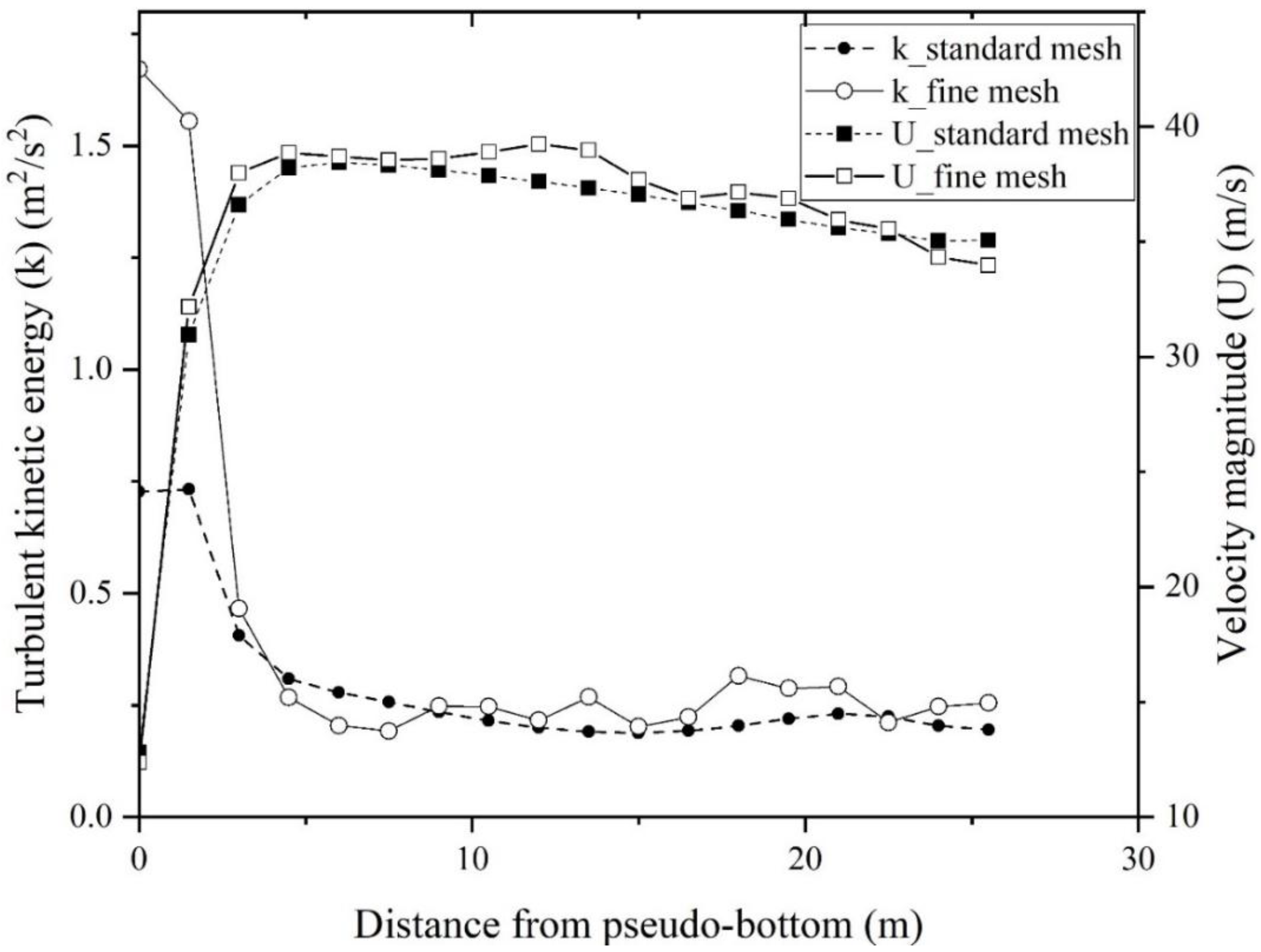
4.1. Mesh Sensitivity Analysis and Model Validation

A mesh sensitivity analysis was carried out for mesh block 2 by using a finer mesh of 0.15 × 0.33 × 0.2 m, i.e., for half the values of the standard cell size. For the finer mesh, only 3% of the discharge difference was found and an identical cavity length (expressed by the number of steps it covered) was obtained. The velocity magnitude (U) and turbulent kinetic energy (k) profiles perpendicular to the pseudo-bottom at the 30th step are presented in Figure 6 for the two meshes, showing only small differences. The larger differences of the near-wall k values result from the FAVOR treatment and wall functions, affecting a flow depth up to about 3 m from the pseudo-bottom, while the effect on the main flow is insignificant. Consequently, the standard mesh was selected for the further simulations due to a significantly less computational cost at high velocity (roughly 40 m/s) two-phase flow.
Load case 3 (see Table 1) was simulated with the numerical model to validate the involved sub-models. The numerical results and experimental measurements of the step surface pressure are shown in Figure 7. It can be seen that the distribution of the pressure, which was obtained by numerical simulation, was similar to that obtained in the lab experiment. The overall difference is around 150 Pa, which corresponds to the range of measuring and numerical errors. The rapid increase of the pressure after step 36 results from the downstream backwater (see Figure 2), whose elevation is approximately 1135m ± 2 m, i.e., at step 35 to 37.
Furthermore, the computed time-averaged discharge is in good agreement with the measurement data (+4.3%), and the size of the aeration cavity (around seven steps) is similar to that observed in the lab experiment. Accordingly, the overall accuracy of the adopted numerical model is good. This is also confirmed by a similar validation of the involved sub-models carried out by Khosro et al. [44] by simulating flow over flat and pooled stepped spillways, where only about a 5% average relative difference of air concentration was found, although no details about the drift-flux model were given.

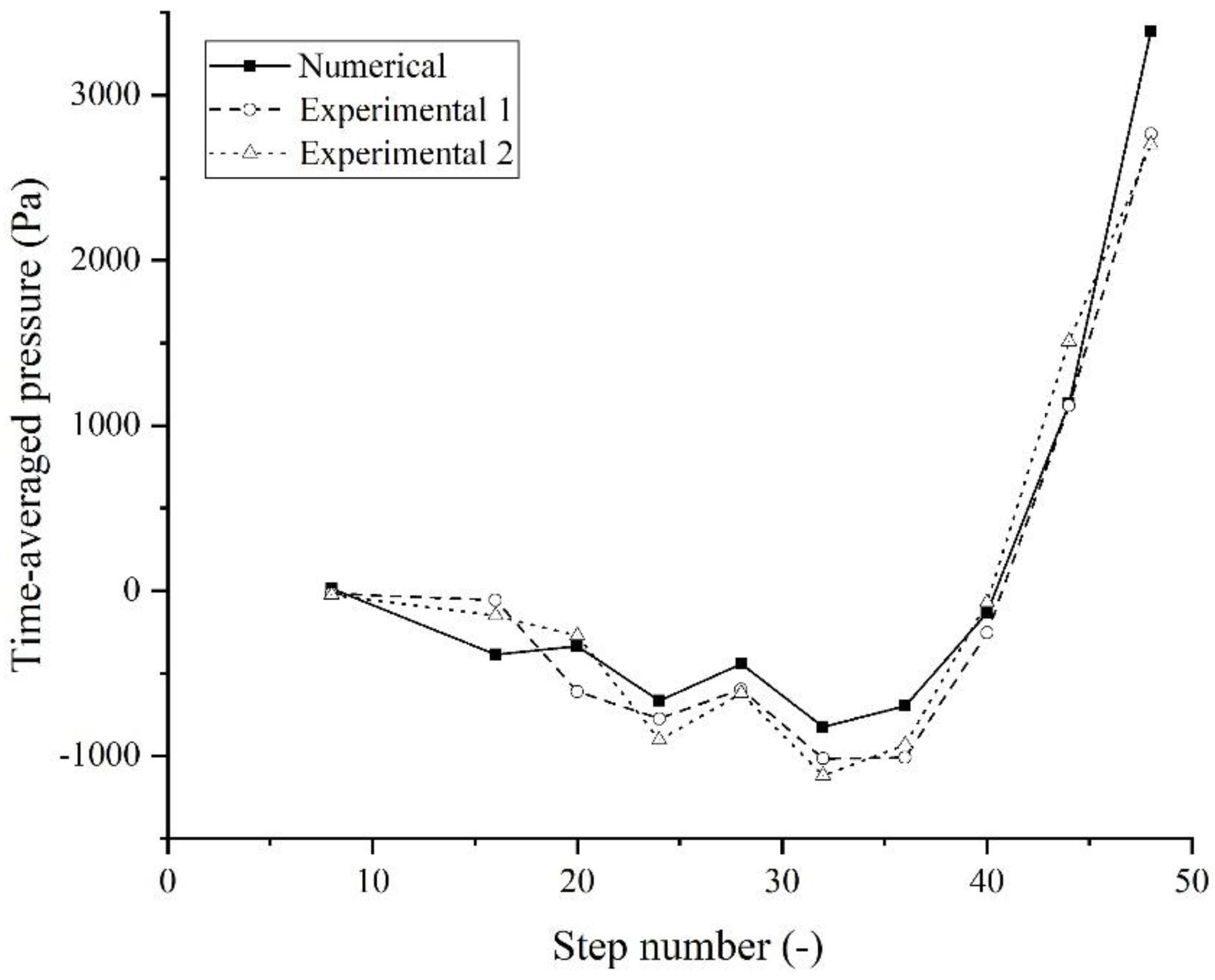
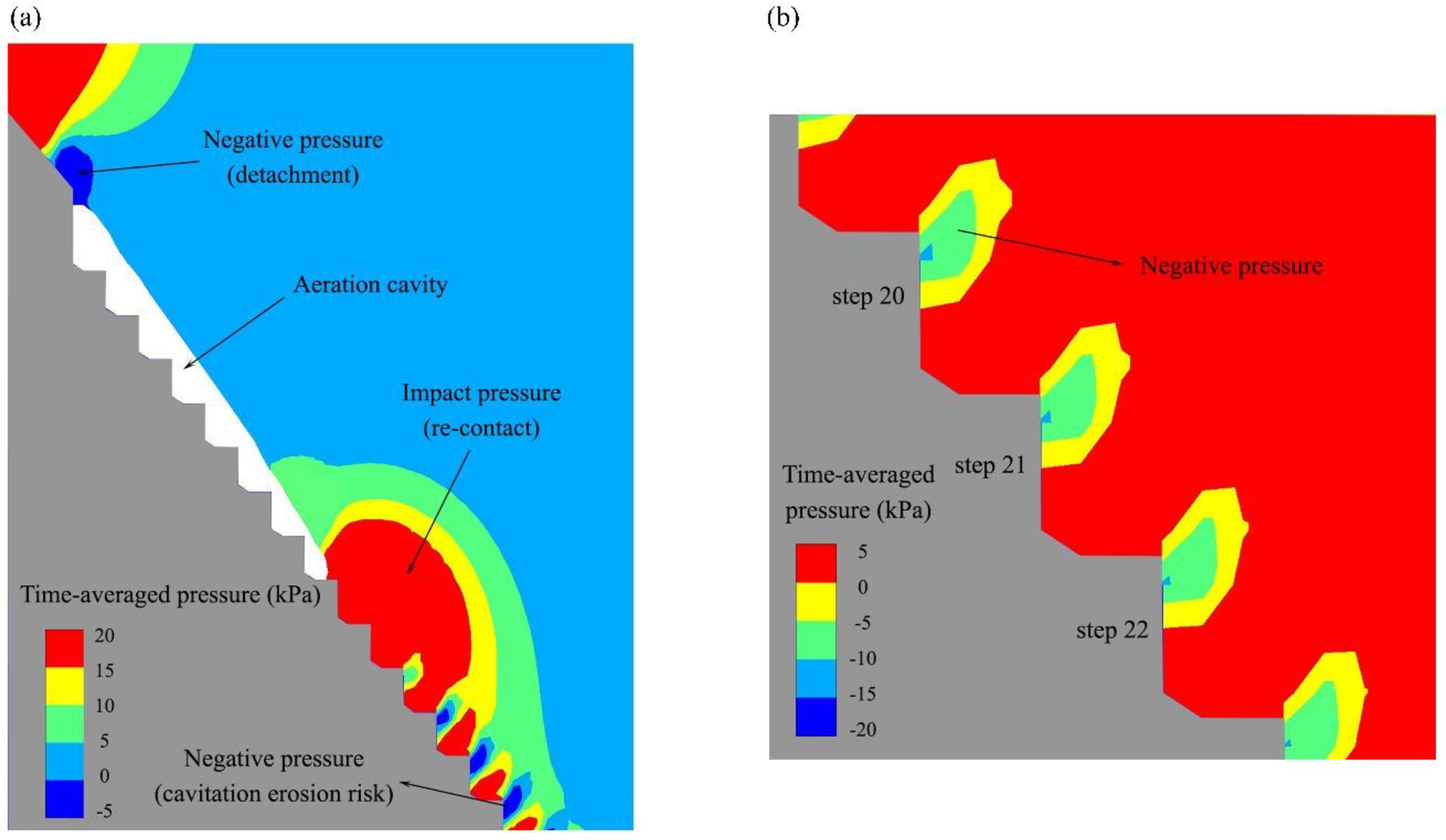
4.2. Pressure Distribution

The pressure distribution above the steps is illustrated in Figure 8. The pressure close to the first 13 steps and the steps 20 to 22 were depicted in detail using different adapted color scales to illustrate positive and negative pressure values. It is revealed in Figure 8a that there is a negative pressure zone at the top of the first step, where the flow detaches from the spillway surface. Upon recontact on the spillway on the eighth step, a large impact pressure is seen. Zhang et al. [25] also found such negative pressure by numerical simulation of the spillway at Suofengying dam with the same type of dissipator and for a similar unit discharge (8% larger than in our current case). They validated their results by corresponding physical model experiments.
In Figure 8b, the negative pressure region in the vicinity of each step tip is clearly visible. Similar pressure was observed by Sánchez-Juny et al.’s and Frizell and Renna’s experimental measurement [5,9]. Because negative pressure on steps may result in cavitation, the cavitation potential will be analyzed in Section 4.4 based on the cavitation index.

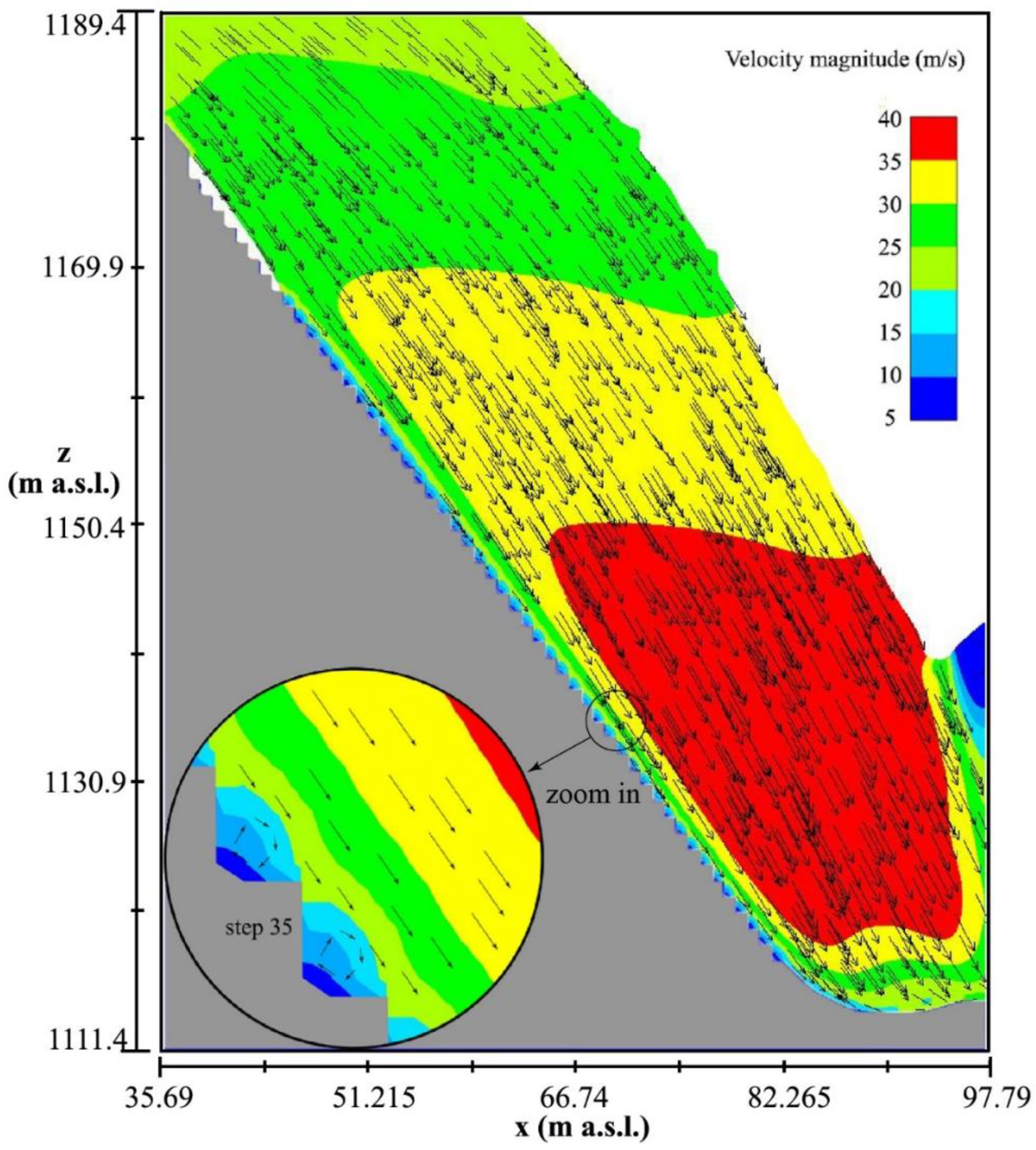
4.3. Velocity Magnitude

The velocity distribution at the axial longitudinal section is shown in Figure 9, where the main flow is approximately parallel to the steps, with a velocity magnitude of some 40 m/s. It can be seen in the enlarged picture (35th to 36th steps) in Figure 9 that in the step niches, the flow velocity is roughly 5 to 20 m/s, and above the pseudo-bottom, the velocity increases rapidly from 20 to 35 m/s within a distance of approximately three step heights. The step surface velocity is about 10 to 15 m/s without much variation, indicating that the pressure plays a more important role in affecting the cavitation index values and thus the cavitation potential.

4.4. Step Surface Cavitation Index

In the presence of negative pressure, high velocity (around 15 m/s), and reduced ambient pressure at the dam site (around 1180 m.a.s.l.), the steps are under high cavitation erosion risk. According to Frizell and Renna’s experimental study [9], the critical cavitation index, σ, for stepped spillways with an inclination angle of 21.9° and 68.1° is about 0.4 and 0.64, respectively. They used the widely known formula as shown in Equation (16) to calculate this cavitation index:
σ = P + P a m b P v p ρ w v 2 2
where σ is the cavitation index, P is the time-averaged gauge pressure, P a m b is the ambient pressure and was selected as 87,932 Pa herein, P v p denotes the vapour pressure (set as 2340 Pa), and ρ w and v are the water density and velocity, respectively. Herein, for a slope of 53°, the critical cavitation index was considered as 0.6. It worth emphasizing that this critical cavitation stands for where the rate of counts of acoustic emissions suddenly changes with decreasing σ , and inception cavitation is expected to occur for our present steps at σ = 1 as summarized in [10].
The damaged region after the 2015 flood at Ludila dam spillway is mainly concentrated at the axial longitudinal section of each surface outlet (see Figure 3a), mostly along steps 30 to 45 (Figure 10), which is called the main damage region hereafter.
Figure 10 presents the cavitation index and air concentration near each step. The cavitation index shows the same trend for the three different load cases: The σ values are almost constant for steps 21 to 35 with values of around 0.3 to 0.5, then they increase until step 45, and finally rise up rapidly from the 45th step to the 50th step. As the flow velocity near the step surface has almost the same value of 10 to 15 m/s in the skimming flow regime [45,46] (as can be seen in Figure 9), the variation of σ is mainly caused by the local pressure changes. The increase of σ after step 35 is likely due to the fact that the step surface pressure becomes larger because of downstream backwater. Note that the discharge only affects the cavitation index within a range of 0.2 to 0.3, and a small gate opening results in relatively small σ values and high cavitation potential. Based on the critical σ value of 0.6, it can be concluded that cavitation damage is likely to occur upstream of the 40th step for all of the three cases.

4.5. Air Concentration

Aeration is a common, efficient, and economical measure to avoid or at least reduce cavitation erosion. The stability of stepped spillways for such high unit discharge relies on the delicate design of the FGP, the bottom aeration at the first step, and the slope break, inducing jet deflection and air entrainment. For the situation at Ludila dam, both self-aeration and bottom aeration exist. The simulated air concentration in the axial longitudinal section is shown in Figure 11, while the air concentration along the steps together with the σ values is presented in Figure 10. According to Peterka [47], air concentration of 5% to 8% is considered sufficient for cavitation erosion prevention. A critical value of 7% was considered herein.
From Figure 10, for load cases 2 and 3, the air concentration near the steps decreases first and then starts to increase in the flow direction, whereas for load case 1, the air concentration increases continuously along the steps, i.e., the air concentration decreases with increasing gate opening and thus unit discharge. That is because a larger opening and the resulting larger nappe depth makes it more difficult for the top surface entrained air to reach the steps. The first damaged step is roughly located at where the step surface air concentration falls below the critical value of 7%. As can be seen in Figure 11a, for case 3, self-aeration occurs already after the FGP, but a sufficient amount of entrained air fails to reach the step surface before approximately the 45th step since the horizontally squeezed nappe is too thick. This may evoke a deeper investigation of the aeration performance of FGP as it was originally designed for enhancing flow turbulence and thus surface aeration while finally it also reduced the steps’ surface air concentration because it significantly thickened the nappe in the middle longitudinal section. On the other hand, a certain amount of air is entrained due to the bottom cavity and then it rises and escapes from the step surface quickly in the following 15 steps. Under the combined effect of these two processes, the air concentration at steps 30 to 45 is not sufficient (i.e., under 7%). This is also shown in Figure 11b by the narrow region in the lower part of the spillway, where the air concentration is lower than the threshold value of 7%. Although this low air concentration region is much narrower than the damaged region, this insufficiency remains responsible for the damage, as normally the main contribution of the so-called cavitation erosion is the consequential vibration of the reinforcement and elutriations induced by the initial real cavitation pitting, as deemed by Peterka [45].

4.6. Aerator Optimization

As mentioned above and depicted in Figure 10 and Figure 11, the air concentration on the stepped surface is locally below the critical air concentration of 7% for the highest discharge, so that cavitation erosion may occur. To improve the current design, a further heightening of the first step was considered to be an economic and efficient measure to entrain more air and thereby maintain more air on the stepped surface. With regard to the slope break between the straight section of the weir and the stepped spillway, a 0.146 m higher first step could be easily gained if the weir crest is extended by one step further downstream ( Δ h = 0.9   × (1/0.75 − 1/0.854) = 0.146 m). The extension of the weir crest by one step (0.9 m) results in a step height of 2.37 m (hereinafter M1) and for two steps (1.8 m) in 2.512 m (hereinafter M2), respectively (see Figure 12).
Figure 13 shows the air concentration distribution at the axial longitudinal section for the original design and the optimized structures M1 and M2. In addition, the air concentrations from the numerical simulations at the axial longitudinal section along the steps for the three above-mentioned designs are shown in Figure 14. It can be seen from Figure 13 that the cavity lengths in M1 and M2 were increased by one step. Consequently, with a higher first step and larger cavity, the step surface air concentration value increases significantly, especially at the upstream region above the 35th step. The lowest air concentration was increased from the original value of 6.1% to 6.7% and 7.7% for M1 and M2, respectively. The results show that heightening the first step is an efficient way for entraining more air and maintaining more air on the stepped surface.

5. Conclusions

The air–water two-phase flow on stepped spillways behind X-shaped flaring gate piers under very high discharge was numerically simulated using the commercial CFD code FLOW-3D®. In doing so, the 3-D Reynolds-averaged Navier–Stokes equations were solved, including the RNG k-ε turbulence model and a VOF method, to capture the free surface. A sub-grid air entrainment model was used in combination with a density evaluation model and drift-flux model to reproduce air entrainment and transport in water flow. The resulting pressure, velocity, and especially air concentration data above the steps were used for further data analysis and validation with data from laboratory experiments. As a case study, the stepped spillway at Ludila dam in southwest China was considered, which underwent damage to the steps in 2015. Finally, the effect of the height of the first step of the spillway on the air concentration along the stepped surface was addressed. The findings of the present research can be concluded as follows:
  • The reliability of the involved models is considered satisfying, as the results are in good agreement with laboratory data.
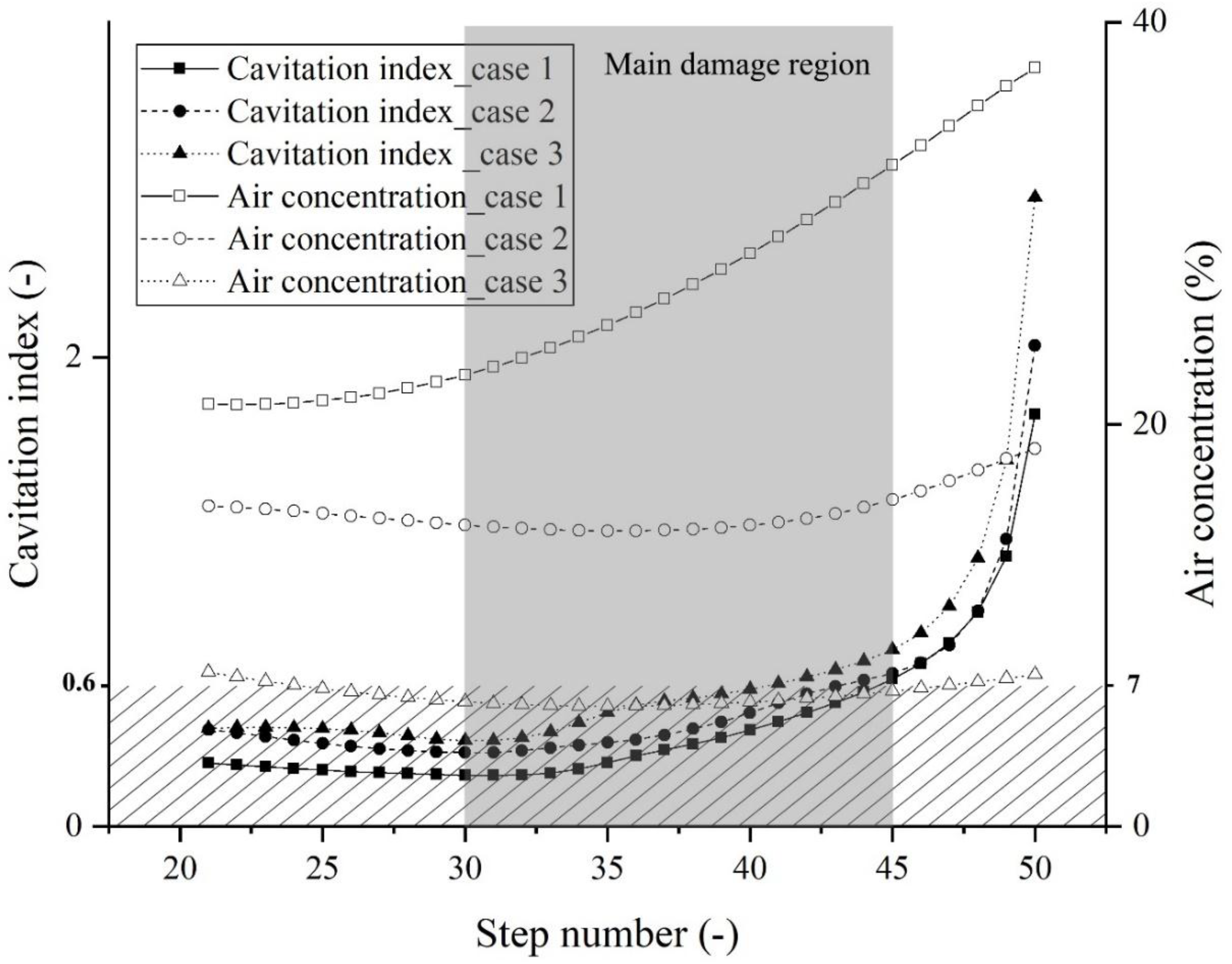
  • The velocity close to the step tips was about 15 m/s, indicating potential cavitation occurrence for all investigated discharges. The negative pressure close to the step tips is a key factor that may cause cavitation erosion, since both analytical evidence of a low cavitation index and practical real-world step failure were discovered.
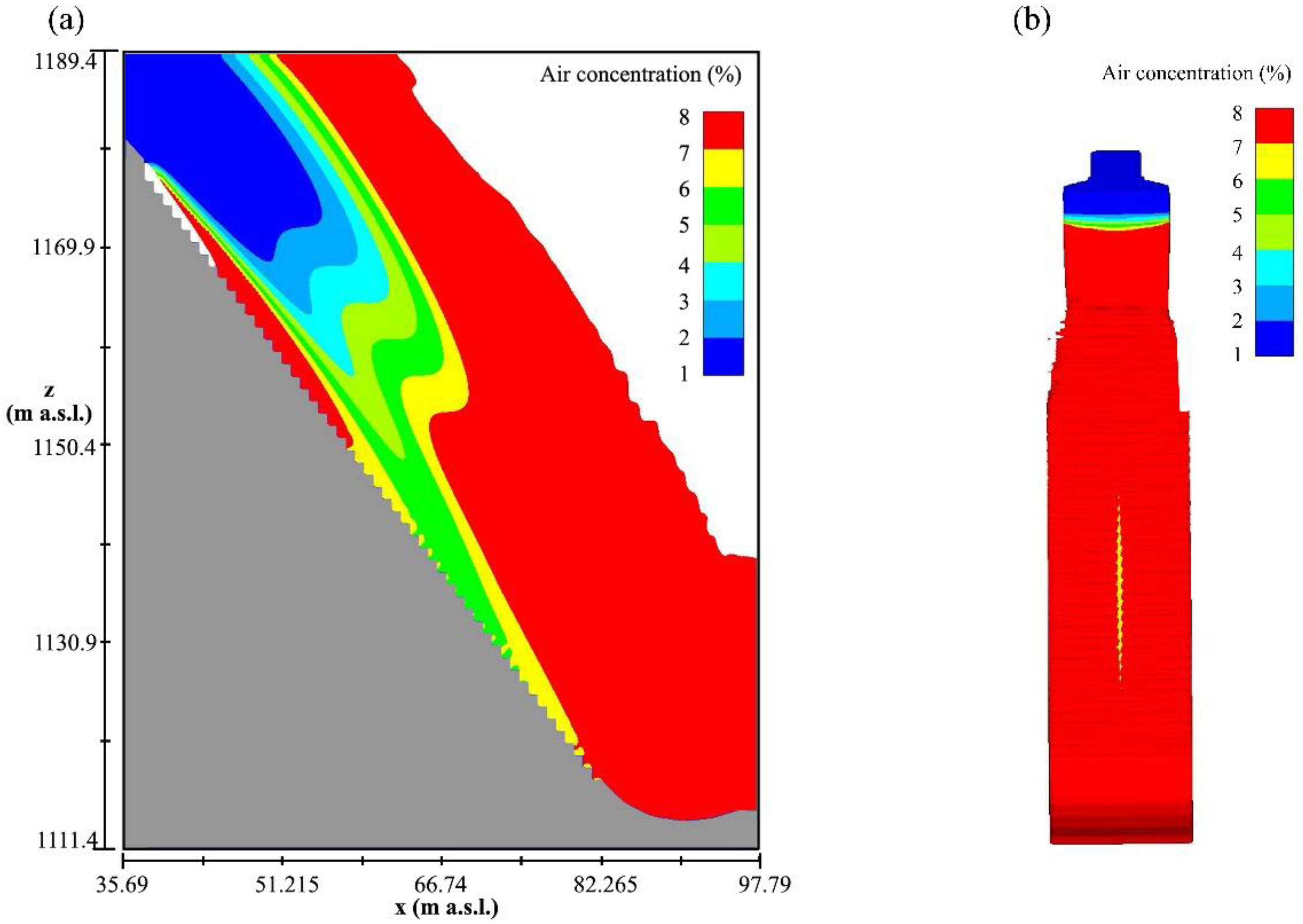
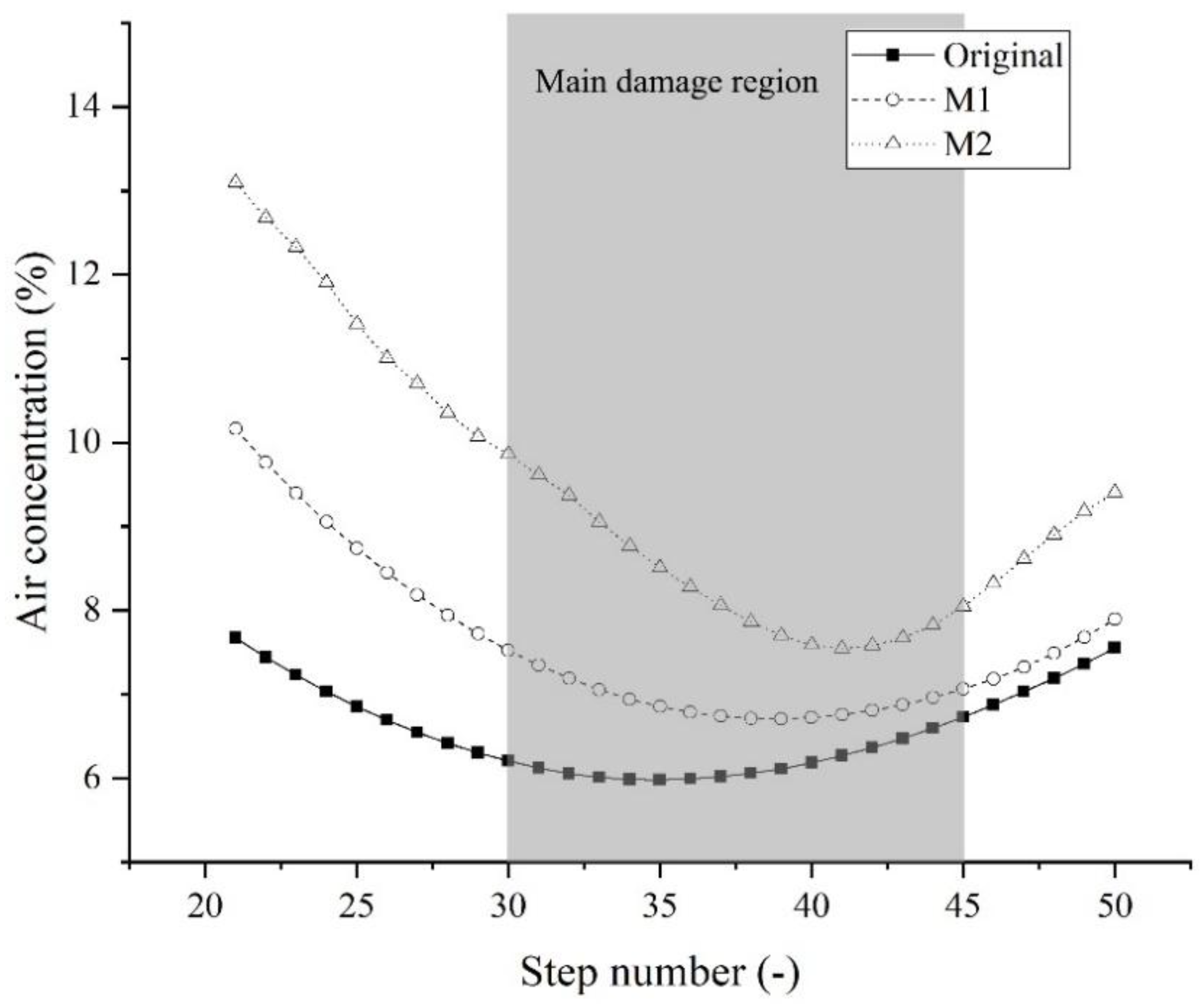
  • The calculated air concentration data is rather reliable, considering the air concentration on the stepped surface behind the X-shaped FGP of roughly 5% to 6% and the reported scaled physical model value of 3% to 5% in [14]. In addition, the simulated air concentration and derived cavitation potential are plausible with regard to the prototype step failure. It was found that for a high unit discharge of 166 m2/s and flow depths up to 30 m (25 times the step height), free surface self-entrained air fails to reach the stepped surface before step 45. A bottom-aeration thus becomes very important but insufficient if a threshold of 7% for the air concentration is considered necessary for cavitation erosion avoidance.
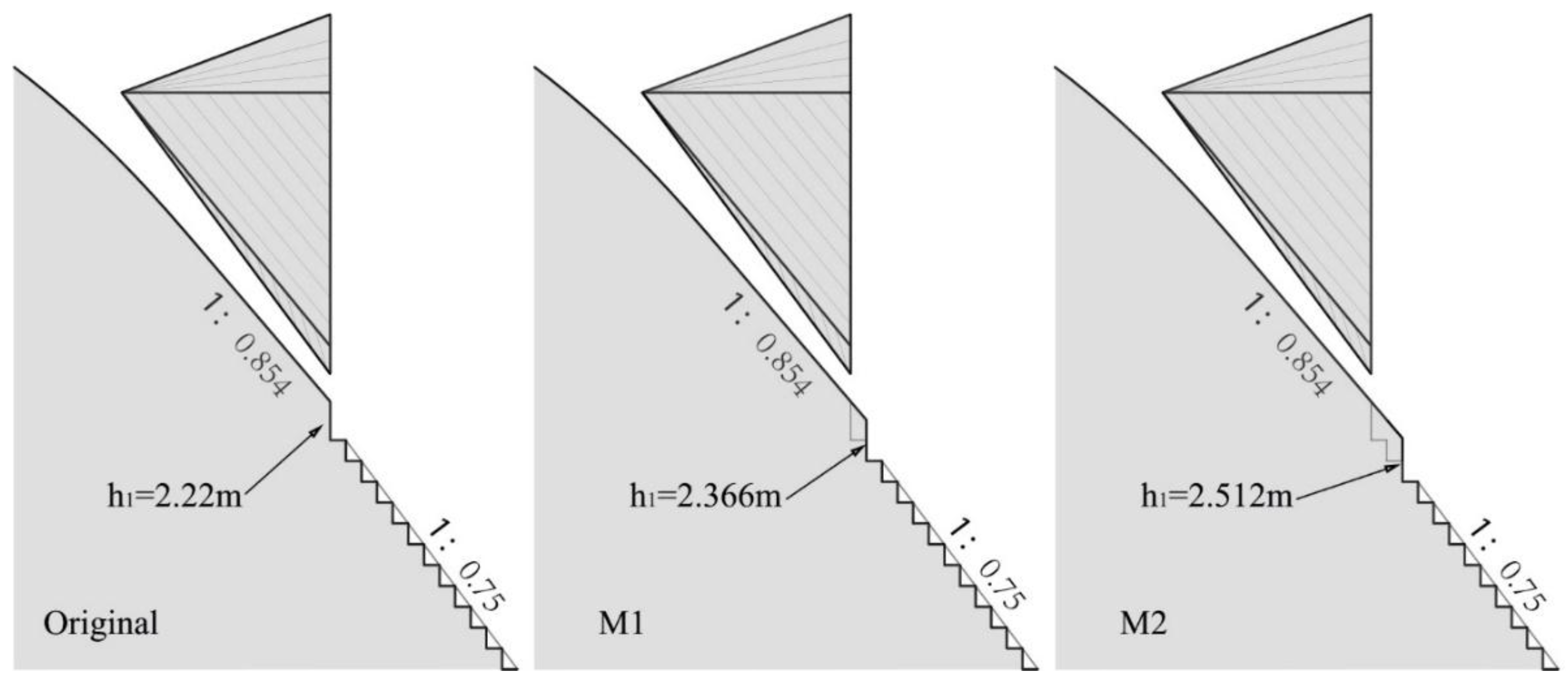
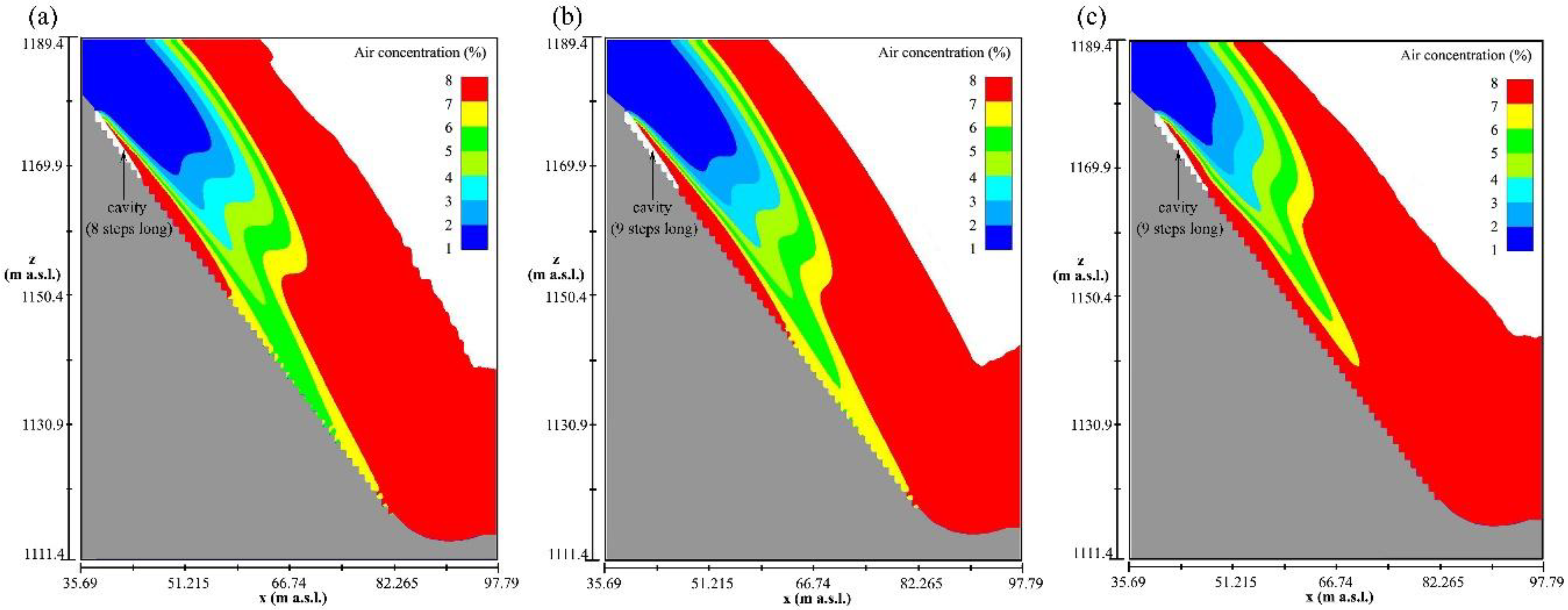
  • The height of the first step of the spillway may affect the air concentration on the stepped surface to some degree. An increased air concentration along the steps for a larger first step height was found in the case study of Ludia dam spillway, especially upstream of step 35. Therefore, for aerator optimization of built projects, heightening the first step could be an economic and efficient measure to prevent cavitation erosion.
However, the present study has some limitations. Air concentration data was not available from the physical model, which would have allowed for further calibration or fine-tuning of the numerical model, especially with regard to the parameters of sub-grid scale models for air-entrainment and transport. Furthermore, fluctuations of pressure and air concentration are also very important, but these remain impossible or at least extremely expensive to acquire for high-velocity two-phase flows. Nonetheless, the findings from the study are encouraging for the use of advanced numerical modelling techniques as used herein for the assessment of the cavitation potential and to propose mitigation measures based on design optimization. This could be of special interest for the operators of more than 10 dam spillways in China featuring a combination of FGPs and stepped spillways, to ensure safe operation and reduce maintenance costs.

Author Contributions

The conceptualization of this research was directed by G.T. and the experimental data was from J.W.; the numerical modelling was performed by Z.D. under the supervision of J.W. and D.F.V.; the manuscript was mainly finished by Z.D., D.F.V. and R.M.B.

Funding

This research received no external funding.

Acknowledgments

The first author would like to thank VAW, ETH Zurich for the computer and software resources and financial support and the China Scholarship Council for the funding of living abroad as an academic guest.

Conflicts of Interest

The authors declare no conflict of interest.

Notation

A p cross sectional area of air bubble (m2)
Asarea of surface disturbance (m2)
C a i r air concentration (–)
C d user-defined drag coefficient (–)
CNUcoefficient equal to 0.09 (–)
d p bubble diameter (m)
D k effective diffusivity of k (kg m−1 s−1)
D ε effective diffusivity of ε (kg m−1 s−1)
eopening of radial gate (m)
fwater volume fraction (–)
gncomponent of gravity normal to the free surface (m s−2)
Hddesign head of weir (m)
Iidentity matrix
K drag coefficient (kg m−3 s−1)
K p drag coefficient for single particle (kg s−1)
k a i r coefficient of proportionality (–)
kturbulent kinetic energy (m2 s−2)
k R Z Richardson–Zaki coefficient multiplier (-)
LTturbulent length (m)
Pgauge pressure in flow field (Pa)
P a m b ambient pressure (Pa)
P k generation of k due to mean velocity gradient (kg m−1 s−3)
P v p vapor pressure (Pa)
Pddisturbance energy per unit volume (N m−2)
Ptdestabilization force per unit volume (N m−2)
qunit width discharge (m2 s−1)
R p bubble radius (m)
u m mixture velocity (m s−1)
u r relative/slip velocity (m s−1)
u r e f f effective relative velocity (m s−1)
U r magnitude of u r (m s−1)
ϑ kinematic viscosity related to the turbulence Schmidt number (m2 s−1)
ϑ e f f effective kinematic viscosity (m2 s−1)
WeWeber number (–)
Zupupstream water elevation (m)
Zdowndownstream water elevation (m)
δ V volume of air entrained to the flow (m3)
Δ h Heightened height when extend curve end 0.9 m downstream (m)
ε dissipation rate of k (m2 s−3)
μ a dynamic viscosity of air (Pa s−1)
ξ 0 Richardson–Zaki coefficient (–)
ρ a density of air, 1.225 kg m−3
ρ m macroscopic mixture density (kg m−3)
ρ w density of water, 1000 kg m−3
σ s u r coefficient of surface tension (N m−1)
τ Reynolds stress tensor (kg m−1 s−2)

Appendix A

Figure A1. Assessment of the convergence to a steady state for case 3: the red line indicates the variation of the total volume of fluid in the domain (Vf), the blue solid line indicates the average of Vf from 90 to 130 s of simulation time; the shaded region (last 10 s of simulation) represents when the numerical data was acquired.
Water 11 01956 g0a1

References

  1. Christodoulou, G.C. Energy dissipation on stepped spillways. J. Hydraul. Eng. 1993, 119, 644–650. [Google Scholar] [CrossRef]
  2. Boes, R.M.; Hager, W.H. Two-phase flow characteristics of stepped spillways. J. Hydraul. Eng. 2003, 129, 661–670. [Google Scholar] [CrossRef]
  3. Boes, R.M.; Hager, W.H. Hydraulic Design of Stepped Spillways. J. Hydraul. Eng. 2003, 129, 671–679. [Google Scholar] [CrossRef]
  4. Chanson, H. The Hydraulics of Stepped Chutes and Spillways; Balkema A.A. Publishers: Lisse, The Netherlands, 2002. [Google Scholar]
  5. Sánchez-Juny, M.; Bladé, E.; Dolz, J. Pressures on a stepped spillway. J. Hydraul. Res. 2007, 45, 505–511. [Google Scholar] [CrossRef]
  6. Ohtsu, I.; Yasuda, Y. Characteristics of flow conditions on stepped channels. In Proceedings of the 27th IAHR World Congress, San Francisco, CA, USA, 10–15 August 1997. [Google Scholar]
  7. Li, B.L. Experimental Study on the Pressure Characteristics in Stepped Spillway; Xi’an University of Technology: Xi’an, China, 2005. (In Chinese) [Google Scholar]
  8. Zhang, J.M.; Chen, J.G.; Wang, Y.R. Experimental study on time-averaged pressures in stepped spillway. J. Hydraul. Res. 2012, 50, 236–240. [Google Scholar] [CrossRef]
  9. Frizell, K.W.; Renna, F. Cavitation potential of flow on stepped spillways. J. Hydraul. Eng. 2013, 139, 630–636. [Google Scholar] [CrossRef]
  10. Boes, R.M. Guidelines on the design and hydraulic characteristics of stepped spillways. In Proceedings of the 24th ICOLD Congress, Kyoto, Japan, 6–8 June 2012; pp. 203–220. [Google Scholar]
  11. Falvey, H.T. Cavitation in Chutes and Spillways. Engineering Monograph 42; Bureau of Reclamation: Denver, CO, USA, 1990.
  12. Pfister, M.; Hager, W.H. Self-entrainment of air on stepped spillways. Int. J. Multiph. Flow 2011, 37, 99–107. [Google Scholar] [CrossRef]
  13. Pfister, M.; Hager, W.H.; Minor, H.E. Stepped chutes: Pre-aeration and spray reduction. Int. J. Multiph. Flow 2006, 32, 269–284. [Google Scholar] [CrossRef]
  14. Liang, Z.X.; Yin, J.B.; Zheng, Z.; Lu, H. Aeration of skimming flow on stepped spillway combined with flaring gate piers. J. Hydraul. Eng. 2009, 40, 564–568. (In Chinese) [Google Scholar]
  15. Pfister, M.; Hager, W.H.; Minor, H.E. Bottom aeration of stepped spillways. J. Hydraul. Eng. 2006, 132, 850–853. [Google Scholar] [CrossRef]
  16. Mateos, I.C.; Elviro, G.V. Initiation of aeration in stepped spillways. In Proceedings of the 27th IAHR World Congress, San Francisco, CA, USA, 10–15 August 1997. [Google Scholar]
  17. Amador, A.; Sanchez-Juny, M.; Dolz, J. Developing flow region and pressure fluctuations on steeply sloping stepped spillways. J. Hydraul. Eng. 2009, 135, 1092–1100. [Google Scholar] [CrossRef]
  18. Xie, X.Z.; Li, S.Q.; Li, G.F. Development of flaring gate piers in China I. Hongshui River 1995, 14, 3–11. (In Chinese) [Google Scholar]
  19. Xie, X.Z.; Li, S.Q.; Li, G.F. Development of flaring gate piers in China II. Hongshui River 1995, 15, 24–30. (In Chinese) [Google Scholar]
  20. He, G.T.; Zeng, X.K.; Li, Z.F.; Yang, S.L. Optimum design of new energy dissipators of Shuidong hydropower station. W. Power 1994, 9, 26–28. (In Chinese) [Google Scholar]
  21. Yin, J.B.; Liang, Z.X.; Gong, H.L. Experimental study on flow characteristics on 3D hydraulic jump of flaring gate piers. J. Hydraul. Eng. 2010, 41, 1333–1338. (In Chinese) [Google Scholar]
  22. Dong, Z.S.; Wang, J.X.; Zhang, W.C.; Da, J.R. Study on dissipation characteristics of incomplete flaring gate pier with low froude number. J. Sichuan Univ. (Eng. Sci. Ed.) 2016, 48, 9–15. (In Chinese) [Google Scholar]
  23. Nan, X.H.; Liang, Z.X.; Liu, H.S. New type of flaring pier for improving energy dissipation of stepped surface overflow dam. J. Hydraul. Eng. 2003, 8, 49–57. (In Chinese) [Google Scholar]
  24. Wang, B.; Wu, C.; Hu, Y.H.; Mo, Z.Y. Relationship of first step height, step slope and cavity in X-shaped flaring gate piers. J. Hydrodyn. 2007, 19, 349–355. [Google Scholar] [CrossRef]
  25. Zhang, T.; Wu, C.; Liao, H.S.; Hu, Y.H. 3D numerical simulation on water and air two-phase flows of the steps and flaring gate piers. J. Hydrodyn. 2005, 17, 338–343. [Google Scholar]
  26. Li, S.; Zhang, J. Numerical Investigation on the Hydraulic Properties of the Skimming Flow over Pooled Stepped Spillway. Water 2018, 10, 1478. [Google Scholar] [CrossRef]
  27. Koh, C.G.; Luo, M.; Bai, W. Simulation of wave impact with compressible air entrainment based on consistent particle method. In Proceedings of the ASME 2015 34th International Conference on Ocean, Offshore and Arctic Engineering, St. John’s, NL, Canada, 31 May–5 June 2015. [Google Scholar]
  28. Wan, H.; Li, R.; Gualtieri, C.; Yang, H.; Feng, J. Numerical simulation of hydrodynamics and reaeration over a stepped spillway by the SPH method. Water 2017, 9, 565. [Google Scholar] [CrossRef]
  29. Zhang, W.; Wang, J.; Zhou, C.; Dong, Z.; Zhou, Z. Numerical simulation of hydraulic characteristics in a vortex drop shaft. Water 2018, 10, 1393. [Google Scholar] [CrossRef]
  30. Chen, Q.; Dai, G.Q.; Liu, H.W. Volume of Fluid Model for Turbulence Numerical Simulation of Stepped Spillway Overflow. J. Hydraul. Eng. 2002, 128, 683–688. [Google Scholar] [CrossRef]
  31. Valentin, H. Scale effects in physical hydraulic engineering models. J. Hydraul. Res. 2011, 49, 293–306. [Google Scholar]
  32. Felder, S.; Chanson, H. Turbulence, dynamic similarity and scale effects in high-velocity free-surface flows above a stepped chute. Exp. Fluids 2009, 47, 1–18. [Google Scholar] [CrossRef] [Green Version]
  33. Takahashi, M.; Yasuda, Y.; Ohtsu, I. Effect of Reynolds number on characteristics of skimming flows in stepped channels. In Proceedings of the 31th IAHR World Congress, Seoul, Korea, 11–16 September 2005. [Google Scholar]
  34. Flow-3D, version 11.2; User Manual; Flow Science Inc.: Santa Fe, NM, USA, 2017.
  35. Yakhot, S.; Orszag, A. Renormalization group analysis of turbulence. I. Basic theory. J. Sci. Comput. 1986, 1, 3–51. [Google Scholar] [CrossRef]
  36. Hirt, C.W.; Nichols, B.D. Volume of fluid (VOF) method for the dynamics of free boundaries. J. Comput. Phys. 1981, 39, 201–225. [Google Scholar] [CrossRef]
  37. Hirt, C.W. Modeling Turbulent Entrainment of Air at a Free Surface; Technical Note FSI-01-12; Flow Science, Inc.: Santa Fe, NM, USA, 2003. [Google Scholar]
  38. Meireles, I.C.; Bombardelli, F.A.; Matos, J. Air entrainment onset in skimming flows on steep stepped spillways: An analysis. J. Hydraul. Res. 2014, 52, 375–385. [Google Scholar] [CrossRef]
  39. Brethour, J.M.; Hirt, C.W. Drift Model for Two-Component Flows; Technical Note FSI-09-TN83; Flow Science Inc.: Santa Fe, NM, USA, 2009. [Google Scholar]
  40. Hirt, C.W. Dynamic Droplet Sizes for Drift Fluxes; Technical Note FSI-11-16; Flow Science Inc.: Santa Fe, NM, USA, 2016. [Google Scholar]
  41. Richardson, J.F.; Zaki, W.N. Sedimentation and fluidisation: Part 1. Trans. Inst. Chem. Eng. 1954, 32, 35–53. [Google Scholar] [CrossRef]
  42. Hirt, C.W.; Sicilian, J.M. A porosity technique for the definition of obstacles in rectangular cell meshes. In Proceedings of the 4th International Conference Ship Hydrodynamics, National Academy of Science, Washington, DC, USA, 24–27 September 1985. [Google Scholar]
  43. Hirt, C.W. Volume-Fraction Techniques: Powerful Tools for Flow Modeling; Flow Science Report FSI-92-00-02; Flow Science Inc.: Santa Fe, NM, USA, 1992. [Google Scholar]
  44. Khosro, M.; Afshin, E. Study of inception point, void fraction and pressure over pooled stepped spillways using Flow-3D. Int. J. Numer. Methods Heat Fluid Flow 2017, 28, 982–998. [Google Scholar]
  45. Rajaratnam, N. Skimming flow in stepped spillways. J. Hydraul. Eng. 1990, 116, 587–591. [Google Scholar] [CrossRef]
  46. Chamani1, M.R.; Rajaratnam, N. Onset of skimming flow on stepped spillways. J. Hydraul. Eng. 1999, 125, 969–971. [Google Scholar] [CrossRef]
  47. Peterka, A.J. The effect of entrained air on cavitation pitting. In Proceedings of the 5th IAHR Congress, Minneapolis, MN, USA, 1–4 September 1953. [Google Scholar]
Figure 1. Schematic of the general flow pattern and aeration mechanism of the stepped spillway combined with X-shaped FGP: (a) 3D air-side view and (b) side view.
Water 11 01956 g001
Figure 2. Longitudinal section of Ludila dam and details of X-shaped FGP.
Water 11 01956 g002
Figure 3. (a) Photo of damaged steps and (b) measured destruction width after the 2015 flood at the Ludila dam spillway.
Water 11 01956 g003
Figure 4. Layout in prototype scale numerical simulation.
Water 11 01956 g004
Figure 5. Geometry and mesh blocks considered for the numerical simulations, including details of the grid resolution at the radial gate lip and spillway steps.
Water 11 01956 g005
Figure 6. Velocity magnitude (U) and turbulent kinetic energy (k) profiles perpendicular to the pseudo-bottom at step 30 in the axis of the longitudinal section.
Water 11 01956 g006
Figure 7. Comparison of experimental and numerical step surface pressure at the middle of the corresponding steps’ vertical faces. Experimental 1 data was measured by rubber piezometric pipe while Experimental 2 data was obtained from a high-speed pressure transmitter.
Water 11 01956 g007
Figure 8. Pressure distribution for case 3 at (a) the 1st to 13th steps and (b) 20th to 22nd steps.
Water 11 01956 g008
Figure 9. Velocity distribution above steps at the axial longitudinal section for load case 3 with details of steps 35 and 36.
Water 11 01956 g009
Figure 10. Air concentration at step surface and corresponding cavitation index along steps 21 to 50 for three load cases: the main damage region between steps 30 and 45 is colored grey and the slash line region stands for cavitation index and air concentration below threshold values of 0.6 and 7%, respectively.
Water 11 01956 g010
Figure 11. Air concentration distribution (a) at the axial longitudinal section and (b) at the stepped surface for load case 3.
Water 11 01956 g011
Figure 12. Design of the original spillway and optimized schemes M1 and M2.
Water 11 01956 g012
Figure 13. Air concentration distribution at the axial longitudinal section for (a) the original design and optimized designs (b) M1 and (c) M2 with an increased first step.
Water 11 01956 g013
Figure 14. Air concentration on the steps’ surface for the original design and optimized designs M1 and M2 with an increased first step.
Water 11 01956 g014
Table 1. Simulated cases.
Load Case No.e (m)q (m2 s−1)
14.7580
29.5120
319166

