Sensitivity Analysis of a Groundwater Infiltration Model and Sea-Level Rise Applications for Coastal Sewers


1
Civil & Environmental Engineering Department and Water Resources Research Center, University of Hawaii at Manoa, 2540 Dole St, Honolulu, HI 96822, USA
2
Urban and Regional Planning, University of Hawaii at Manoa, 2540 Dole St, Honolulu, HI 96822, USA
3
AECOM, 1001 Bishop St, Suite 1600, Honolulu, HI 96813, USA
*
Author to whom correspondence should be addressed.
Water 2020, 12(3), 923; https://doi.org/10.3390/w12030923
Submission received: 24 December 2019
/
Revised: 14 March 2020
/
Accepted: 20 March 2020
/
Published: 24 March 2020
(This article belongs to the Section Hydraulics and Hydrodynamics)
Abstract
:Groundwater elevations in coastal cities will be affected by climate-change-induced sea level rise (SLR) and wastewater collection systems will experience increased groundwater infiltration (GWI) due to greater submergence of sewer pipes. Commercial sewer hydraulics models consider GWI to be a constant quantity estimated via a low-flow monitoring campaign and are incapable of predicting future flows due to changes in GW elevations. A global sensitivity analyses conducted for a two-dimensional GWI pipe flow model found the most important input parameters are groundwater head and surrounding soil hydraulic conductivity. Two case studies were conducted considering a range of pipe defect severity to estimate increases in GWI associated with predictions of future SLR. The findings are that SLR will begin to have noticeable impacts in terms of increased average dry weather flow (ADWF) as soon as 2030 (3–10%) and will increase dramatically in the future (10–29% by 2050, and 50% or more by 2100). Daily and seasonal tide ranges affect the normal diurnal flow variations by between 3% and 10%. The estimation methodology and case studies described here illustrate the coming future importance of SLR effects on GWI in coastal collection systems that should be included in facilities planning and design.
1. Introduction
Inflow and infiltration (I/I) describe the extraneous sources of water which enter a sewer collection system and contribute to wastewater flows. I/I water originates from non-wastewater sources, including improper yard/roof drains, groundwater, and percolating rainwater components. Priority areas for managing I/I include low-lying areas, areas with unstable soils, areas with high groundwater, old pipe infrastructure, sewers located near storm drains, and sewers located near bodies of water. For collection systems with excessive I/I flows, potential impacts are sanitary sewer overflows (SSOs) from overloaded manholes and pump stations, and increased risk of bypasses at the wastewater treatment plant if flow capacity is exceeded [1,2,3].
Sea level rise (SLR) is occurring as a result of ocean thermal expansion and the melting of land-based ice [4]. As the sea-level rises, forcing of the freshwater-saline water interface occurs in coastal/shoreline areas and soil becomes more saturated [5]. The water table is elevated towards the ground surface and reduces the unsaturated zone; when it exceeds ground level, groundwater inundation occurs [6,7]. This phenomenon can already be observed in places like Honolulu during very high tide events, including, but not limited to “king tides”.
For groundwater levels near the coast of New Haven, Connecticut, MODFLOW simulations of long-term future groundwater demonstrate water tables rising 0.9 m in response to a 0.9 m sea-level rise scenario (as predicted for the year 2100); groundwater levels were predicted to rise even where water tables were already 5.2–7.3 m above the current sea level [5]. In the caprock aquifer of Waikiki in Honolulu, HI, approximately 1.1% of a 13 km2 study area currently has an unsaturated zone depth of less than 0.33 m; with a sea-level rise scenario of 0.98 m, 19.3% of this area will have an unsaturated depth less than 0.33 m [7]. In the long-term, the magnitudes of sea-level rise and coastal groundwater-table rise will be equal [7]. Flood conditions will intensify when high tides and heavy precipitation events are concurrent for unconfined aquifers [6]. Projected heights of sea-level rise for Honolulu are 0.18–0.37 m by 2030, 0.40–0.88 m by 2050, and 1.2–3.3 m by 2100 [8].
In coastal areas, many subsurface wastewater pipes are already partially or completely submerged in groundwater and as SLR occurs these pipes will become more submerged and additional pipes will be submerged increasing groundwater infiltration (GWI). Groundwater infiltration is affected by soil type (hydraulic conductivity), pipe and lateral continuity (holes, cracks, poor connections), and sewer system depths relative to groundwater levels (head pressure on submerged pipes) [9]. Methods for estimating GWI in practice include direct measurement, inferred estimation, water consumption analysis, and treatment plant flow-based estimates [10]. GWI can be estimated by subtracting base sanitary flow from total flow measured during dry weather days. Average nighttime low flows, minus known industrial or commercial flows, can also be used to estimate GWI. Commercial sewer hydraulic models rely on these estimation methods and are not capable of “calculating” infiltration due to hydraulic head because normally it is not necessary. However, future SLR will change GW head in coastal areas and thus a calculation method is needed.
The broad classifications of numerical sensitivity analyses are local and global methods. Local methods assess the effect of perturbing an input on the change in the output by varying inputs one-at-a-time (OAT) [11]. Local methods are conducted by computing partial derivatives for the output with respect to input variables. The process varies one input while all other inputs are held constant for a selected baseline value. Inputs are varied by a small fractional change interval around a determined baseline value; the small intervals for perturbing the input are typically the same for all inputs. Global sensitivity analysis methods (GSA) apportion uncertainty in the output to uncertainty in the input parameters through the consideration of probability distributions which cover the entire possible range of values for the input [11].
There are two key characteristics for global methods: first, sensitivity estimates of input parameters require ranges and distributions; secondly, sensitivity estimates of input parameters are evaluated while all other factors are also varying [11]. A first-order (main effect) sensitivity index of an input factor is defined as the fractional contribution of the input factor variance to output variance. Higher-order indices include interaction effects for the inputs. Therefore, total sensitivity indices include all interactions for the total effect of an input factor. Sensitivity indices can be implemented to rank the influence of input parameters as a metric for importance.
Based on studies that predict substantial groundwater inundation due to SLR in coastal environments, there is a need to make quantitative estimates of GWI increases in susceptible sewer networks. In this work we first conduct a sensitivity analysis of an equation to estimate GWI, then we develop case studies of the wastewater system in Honolulu, HI using methods that are applicable to any coastal sewage collection system. In the case studies, we calculate GWI for various hypothetical scenarios that consider SLR and pipe conditions (crack size and percent of pipes cracked).
2. Materials and Methods
A two-dimensional approximate solution for GWI into a sewer pipe is shown in Equation (1) [12]. Equation (1) assumes Darcy’s Law governs flow through porous media and considers orifice flow into a pipe. The input parameters which can be evaluated in a sensitivity analyses are sewer radius (r), sewer defect size (β), defect location on the pipe circumference (α), wastewater head above the pipe defect (Pi), groundwater head above pipe center (h) and hydraulic conductivity of the surrounding soil (K). This equation models the flow through a uniform crack (with an opening size of β) along the full length of the pipe. The equation can be used to evaluate the effects of SLR-induced increases in groundwater head on GWI. If flow monitoring data are available and the GWI flowrate can be identified for a known branch of a collection system, then a calibration of this model could be conducted.
with
where:
- Q = inflow rate per unit length of pipe (m3 day−1 m−1)
- K = hydraulic conductivity of the surrounding homogeneous soil (m day−1)
- h = groundwater head above pipe centerline (m)
- Pi = internal pressure head due to depth of water above defect, equal to atmospheric pressure (Pii = 0) when defect is above the content level or pipe is empty (m)
- β = defect size, expected to be small (0–π/18) otherwise soil particles wash into pipe (0–π/18) (radian)
- r = pipe radius (m)
- α = defect location (0–2π) (radian)
The R sensitivity package includes the Sobol–Martinez method which can be used to calculate Sobol sensitivity indices [13]. This method implements Monte Carlo estimation of Sobol indices for the first and total indices using correlation coefficient-based formulas. The Sobol–Martinez Method is based on Standardized Regression Coefficient (SRC) methods [14]. With SRC methods, the Sobol index is equal to the coefficient of the correlation between random variables. Consequently, the Sobol index is also equal to the ratio between the covariance of the variables. Covariance is estimated empirically from the sampling of two random variables, with two random samples of input factors required. In order to calculate confidence intervals for the sensitivity indices, Sobol–Martinez implements the Fisher Transformation. It has been tested with non-monotonic functions and will accommodate nonlinear functions. The total cost of the Sobol–Martinez model is (p + 2) × n, where p is the number of inputs and n is the random sample size.
The function for analysis is the two-dimensional approximate GWI solution (Equation (1)). To meet the requirement for input factors, two random samples are used. The identified random sample size is set as n = 2000 and the default confidence level (0.95) is applied. The Sobol–Martinez method is useful for the function since it supports missing values and allows for the consideration of only real values of GWI generated by the two-dimensional approximate model. First-order and total sensitivity indices will rank all of the input parameters.
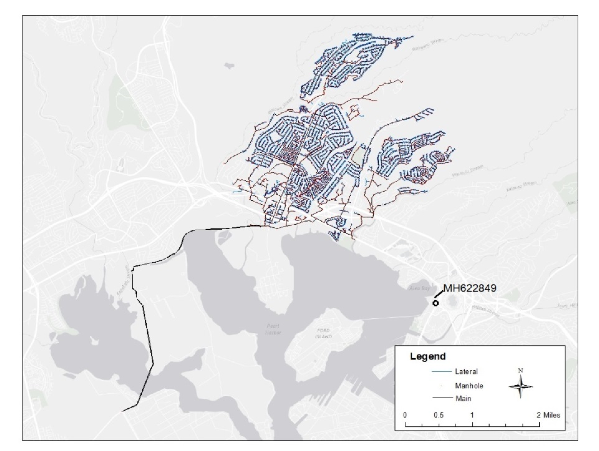
The control area used for sewer system data as inputs to conduct the sensitivity analyses was the Pearl City area on Oahu, HI which is located over a portion of the Pearl Harbor aquifer (Figure 1). The Pearl Harbor aquifer is classified as an unconfined basal aquifer composed of highly permeable basalt [15]. All input parameters were assumed to have a continuous uniform distribution, a normal practice for global sensitivity analyses [16]. The uniform distribution assumption is also substantiated by the understanding that identifying reasonable ranges of input parameters is generally more important than the assigned distributions [11].
Hydraulic Conductivity (K): Based on well draw-down data for the greater Pearl City area, the hydraulic conductivity varies widely from 7.9 to 25,908 m day−1 (26 to 85,000 ft day−1), for Well 2356-54 and Well 2300-22, respectively [17].
Groundwater Head (h): The maximum groundwater head would correspond to groundwater fully inundated to the ground surface and thus the range corresponds to the minimum and maximum manhole depths in the control area which are 1.0 to 9.3 m (3.3 to 30.5 ft).
Pipe Radius (r): The documented pipe radius data range for the control area [18] is 0.102 to 1.22 m (4 to 48 in).
Defect Size (β): Equation (1) accommodates a small range for defect size (β), because soil particles may wash in when the defect is too large, changing the hydrodynamic behavior at the defect. The applicable defect size range has been suggested as π/180 to π/18 [12].
Defect Location (α): Defect location may be sampled at any point along the circumference of the pipe from 0 to 2π. All points are included along the entire pipe wall, including the crown, invert, and springline.
Internal Pressure Head (Pi): A methodology for determining internal pressure head above the defect is required, since the value depends on both the content level of the sewer and the defect location. The new parameter introduced for this input factor is pipe content level. It is assumed that the pipe content level could be empty to completely full. The defect location value converts the radian value to Cartesian, rsin(α). The defect location and content levels are then compared. If content is below the defect then Pi must equal zero. If content is above the defect, the difference of the content level and defect location is calculated to determine pressure above the defect. A uniform distribution is applied to each of the parameters in this GSA assuming a constant probability of values within the ranges cited above.
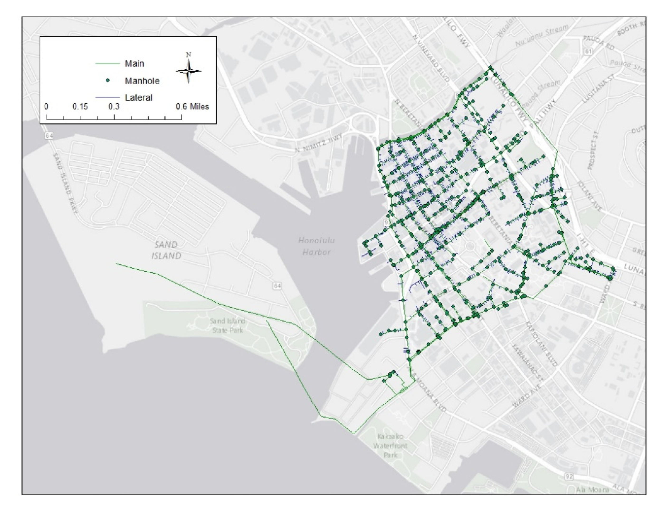
The theoretical consequences of SLR on GWI into a coastal sewer collection system were investigated for downtown Honolulu (Figure 2) using system data available online (GIS.hicentral.com/pubwebsite/). The case study area is a dense urban area previously determined as vulnerable to sea-level rise induced groundwater inundation [6].
The total length of pipes in this study area is 53,116 linear m (174,264 linear ft). Bounds include Ala Moana Blvd., Honolulu Harbor, Nuuanu Stream, South School St., the H-1 freeway, Ward Ave, South Beretania St., and South St. Pipe segments are located within approximately a 2 km2 area (0.8 mi2). This system is serviced by the Sand Island Wastewater Treatment Plant (SIWWTP), and a sewer main to SIWWTP is included in the case study. The average hydraulic conductivity of the downtown Honolulu area is 30 m day−1 (99 ft day−1) [19].
In the absence of pipe condition observations, a range of hypothetical pipe condition scenarios were developed for the assessment. Defects are assumed to be located at the crown (π/2) and internal pressure head is assumed to be zero (Pi = 0, defect is located above wastewater level in the pipe). A range of defect sizes is considered, from Mild (π/90) to Moderate (π/30) to Severe (π/18). Similarly, a range of how many pipes have defects was considered, from Mild (5%) to Moderate (30%) to Severe (75%). These two ranges are combined into a severity matrix of conditions that allows consideration of 9 cases (Figure 3).
The temporal variation of groundwater due to ocean tides and its impact on GWI was studied at a manhole (MH 622849, see Figure 2) less than 35 m from the shore of Pearl Harbor, HI. For this location, the assumed hydraulic conductivity value is 93 m day−1 (305 ft day−1) at Well 2255-35 [17]. The pipe diameter connected to the manhole is 0.762 m (30 in) and the pipe invert is at 2.17 m (7.1 ft) above mean sea level (MSL). It is further assumed that the pipe is empty (Pi = 0) and contains a hypothetical mild defect (β = π/90, a 1.3 cm crack).
Tide levels relative to MSL are from the Ford Island Ferry NOAA tide station [20]. Groundwater data for the case study site are available nearby at the Aiea US Navy 187-B [21]. Daily average groundwater observations are attributed at midday for convenience. Both short-term (1 September @ 0:00 (t = 0 h) to 30 September 2015 @ 12:00 (t = 708 h)) and long-term variations (1 September 2014 (t = 0 h) to 6 October 2015 (t = 9612 h)) were considered for this case study.
3. Results
3.1. Sensitivity Analyses
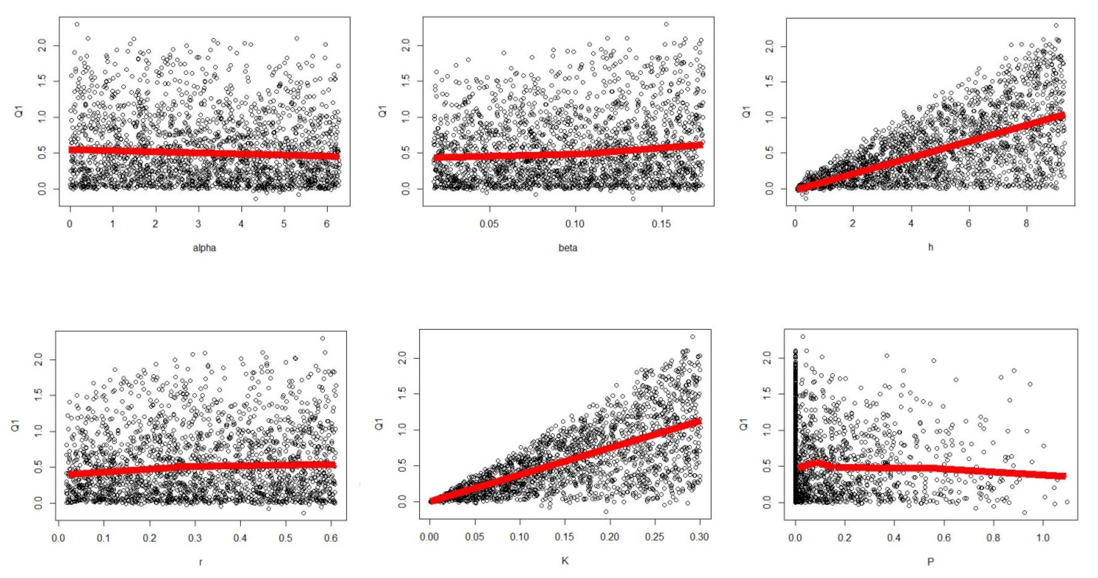
Scatter plots are used to visualize the GWI results as a function of the six input parameters (Figure 4). A smooth curve computed by locally weighted smoothing (LOWESS) is added so trends are evident. As the GSA method varies all parameters for each random sample, the results demonstrate the GWI model behavior. As hydraulic conductivity (K) increases the GWI rate (Q1) increases. A noticeably similar pattern is evident for groundwater head (h), where GWI rate increases as the groundwater elevates. There is no apparent trend for defect location (α). For the internal pressure head (P), there is a high density at Pi = 0, since the pressure is taken as zero for every time the sampled content level is below the sampled defect location. Upon visual inspection, the inputs of defect size (β) and pipe radius (r) show no clear influence on GWI rates.
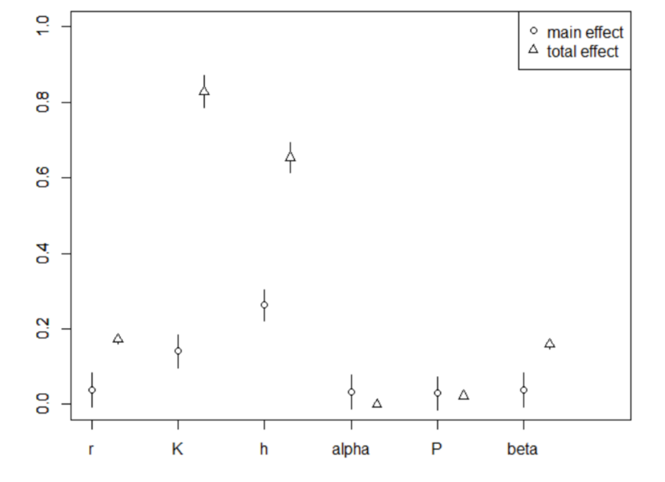
Figure 5 shows the computed Sobol–Martinez sensitivity indices. At the sample size n = 2000, the parameter ranking for first-order, main effect on GWI is: groundwater head, hydraulic conductivity, radius, defect size, defect location and internal pressure head. The main sensitivity index for groundwater head is 0.264 and the index for hydraulic conductivity is 0.14. The main sensitivity indices for defect angle, defect location, pipe radius, and internal pressure head are all much smaller (between 0.03 and 0.04). When considering total effect interactions, the parameters demonstrate a slightly different rank: hydraulic conductivity, groundwater head, pipe radius, defect size, internal pressure head, and defect location. Hydraulic conductivity has the largest total effect index (0.83) and the smallest total index is for defect location (0.00). Individual (first-order) analyses calculate the single parameter variance over the output variance. The total sensitivity is the ratio of the single parameter variance plus the sum of the variances of the input parameter with each of the other input parameters divided by the output variance. The total index considers all the interactions between the input variables while the first-order analysis ignores the interactions. Both main and total indices are useful to determine the sensitivity of the input parameters on the output and therefore where the highest quality input data is required. The two sets of indices provide a check on each other. The sensitivity analyses indicate that the most important parameters to have good estimates for are h and K in order to accurately estimate GWI.
3.2. Large Area Case Study
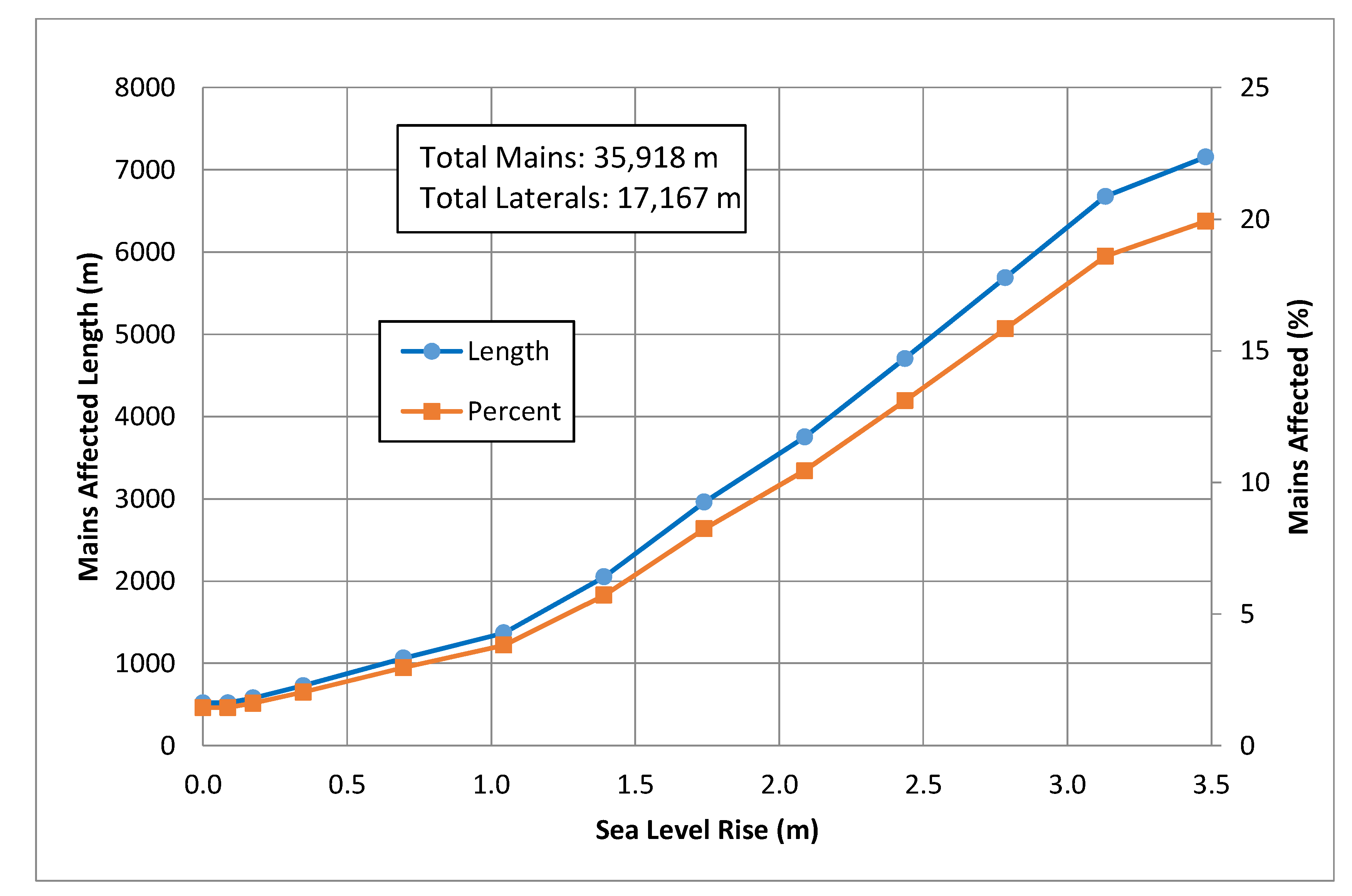
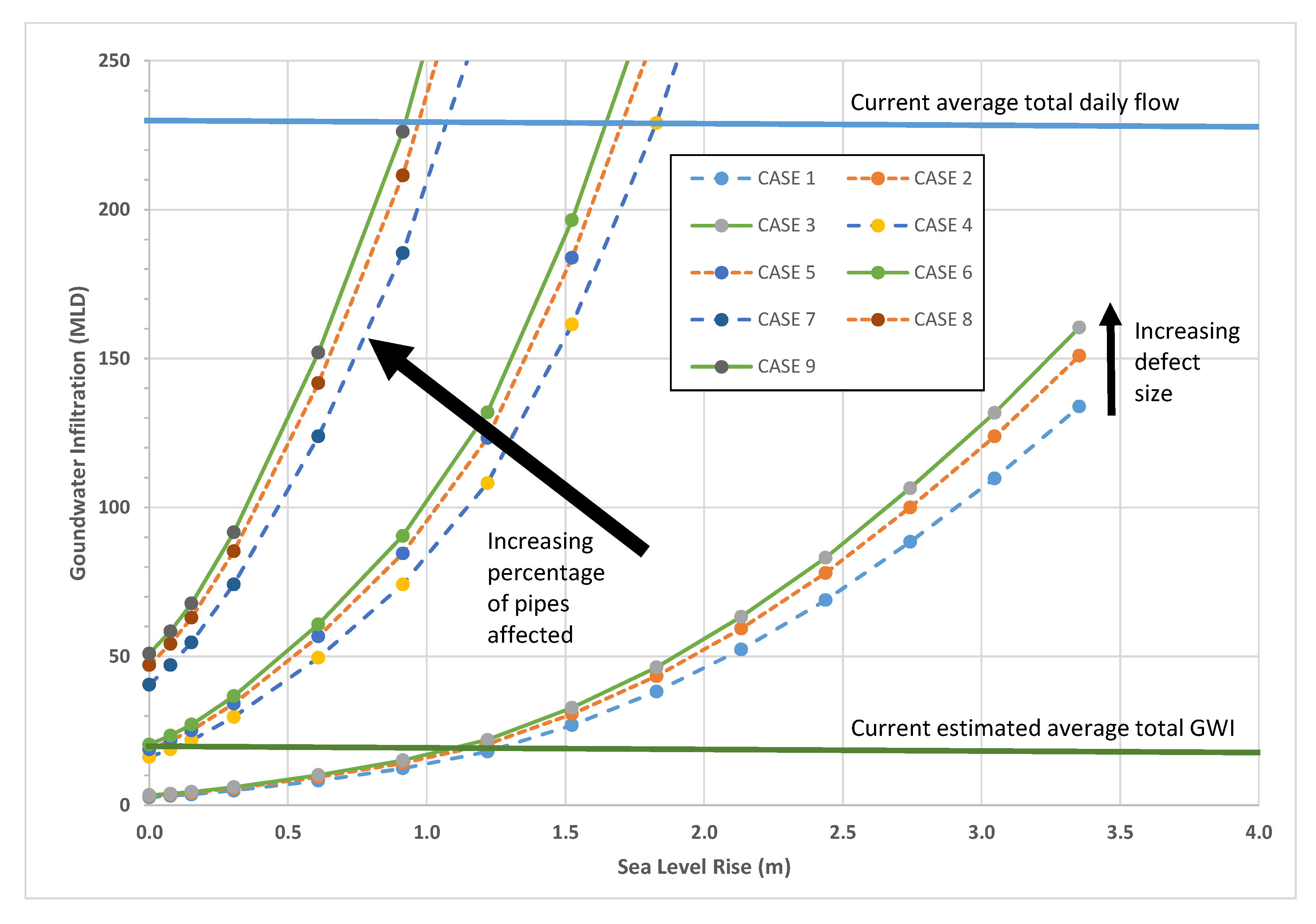
The length of pipe submerged or partially submerged by SLR for the Downtown Honolulu case study is shown in Figure 6. These results indicate that 520 m of pipes are currently submerged and that with 1 m SLR, it will increase to 1370 m of pipe and 6300 m of pipe with 3 m of SLR (compared to the total length of 35,918 m). The rate of GWI as a function of SLR (Figure 7) is restricted to groundwater hydraulic head no greater than 3 m (10 ft.) above all the system pipe centerlines since the case study area sewers do not exceed this buried depth. For this analysis, the GWI for each individual pipe length (mostly 3.2 m or 10 ft each) is calculated and then summed. The value of K is assumed constant for all pipe sections (30 m day−1). The defect location is assumed to be the sewer crown and the value of Pi is assumed to be zero (worst case scenario). The behavior of the GWI is non-linear as a result of the natural logarithm argument of the model approaching zero (where the ratio between the groundwater hydraulic head and pipe radius is one and the defect is at the crown).
In Figure 7, the various severity cases form three groupings (1-2-3, 4-5-6, and 7-8-9) based upon the percentage of pipes affected by SLR; 5%, 30%, and 75%, respectively. Within the three groupings, there are three values of defect size; Mild (π/90), Moderate (π/30) and Severe (π/18). Figure 7 shows that the effect of defect size on GWI is smaller than the effect of percentage of pipes affected. To put the predicted GWI in perspective, the current estimated total GWI for the system is shown as 20 million L day−1 (MLD) as well as the total current average daily flow treated at the wastewater treatment plant (WWTP) (230 MLD); thus, the GWI is currently less than 9% of the average dry weather flow (ADWF). Also, the maximum flow capacity of the WWTP is 910 MLD. The current estimated GWI for this system with zero SLR (20 MLD) is quite close to Cases 4 (16 MLD), 5 (19 MLD) and 6 (20 MLD) which corresponds to 30% of pipes affected. As SLR increases, the amount of GWI will increase significantly and cause a concomitant increase in ADWF to the WWTP which will increase treatment costs, energy use and potentially impact compliance with the facility’s discharge permit. Table 1 shows the predicted future GWI and ADWF values due to the predicted ranges of SLR for Honolulu (0.2 to 0.4 m by 2030, 0.4 to 0.88 m by 2050 and 1.2 to 3.3 m by 2100). Table 1 shows that the ADWF could increase 3.5% to 10.4% by 2030, 8.7% to 29.1% by 2050, and 39% to 48% or more by 2100. These numbers can be used by the wastewater utility for planning purposes.
3.3. Tidal Effects Case Study
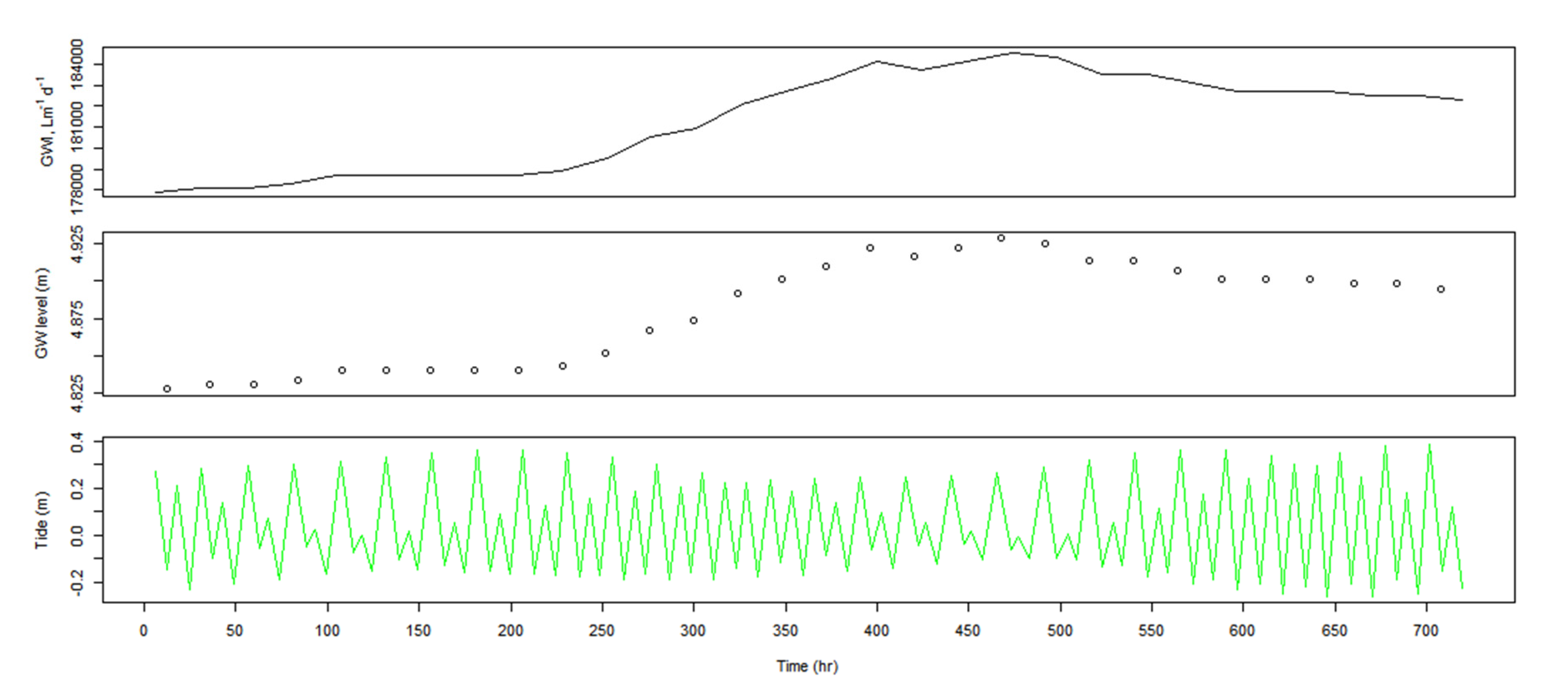
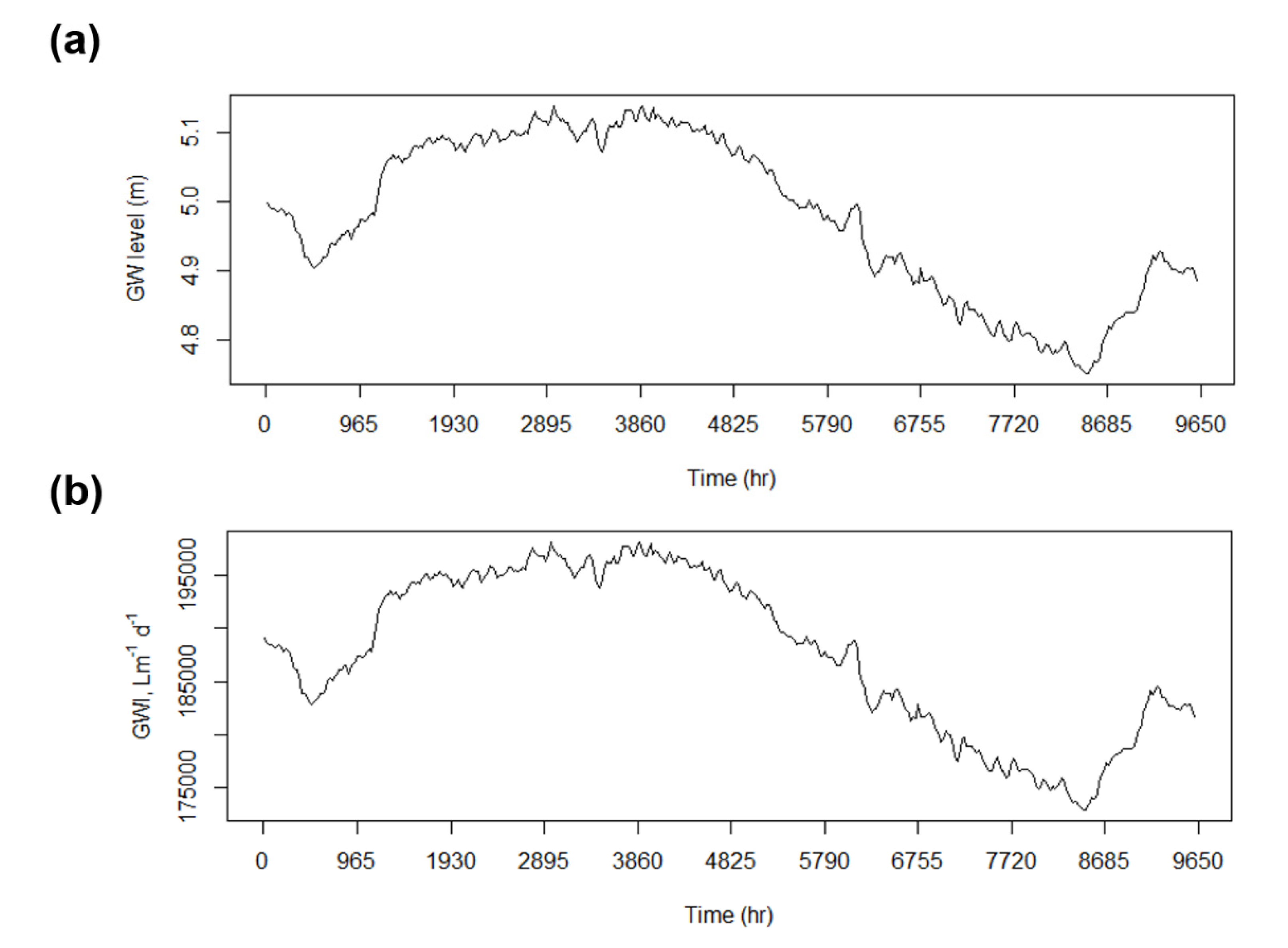
The effects of tide on GWI (assuming a mild defect, β: π/90) were examined for a one month period (1 September 2015–30 September 2015, 720 h; Figure 8) and for a one-year period (1 September 2014–6 October 2015, 9612 h; Figure 9). The monthly signal exhibits mixed semidiurnal tidal period behavior (recorded above MSL datum). The highest tidal magnitude (0.387 m) is observed at 702 h (September 30), and the lowest magnitude (−0.262 m) occurs both at 646 hr and 670.5 h (September 27 and 28, respectively). Groundwater level reaches its maximum (4.93 m above MSL) at 468 h (September 20). The groundwater variation observed for this month results in GWI ranging from 178 to 185 m3 day−1 m−1. The maximum GWI increase (7 m3 day−1 m−1, 564 gal day−1 ft−1) is fairly small because the maximum tidal variation at this manhole location for this time sequence is 0.1 m (4 in). The annual data set (Figure 9) exhibits a seasonal tidal effect with the GWI rate highest in January (2964 h on January 2) and lowest in August (8460 h on August 19). Here the groundwater head difference is larger at 0.38 m (15 in) resulting in a somewhat more significant GWI increase of 25 m3 day−1 m−1, (2013 gal day−1 ft−1) between the extreme low and high values.
The effects of tide on GWI might seem small, however, this analysis is for a single pipe and the overall differences in GW elevation (0.10 to 0.38 m) are what is important. This range is the same as the projected SLR for 2030 for Honolulu and resulted in estimated GWI difference of 24–30 MLD, which is 3.5–4.3% increase in ADWF (Table 1). This would be the daily difference between maximum and minimum rates that would be observed at the affected pump stations that supply the WWTP and the headworks at the facility. These daily peaks would sometimes be in phase with the daily diurnal flow peaks and other times would be out of phase.
4. Discussion
A two-dimensional model [10] has been used to estimate GWI variation due to rising GW elevations in coastal sewer systems due to SLR as a function of soil type and defect size. Manipulation of the hydraulic head parameter (h) replicates scenarios of elevated groundwater due to SLR to facilitate planning for future increases in flow and mitigation measures such as sewer rehabilitation and/or capacity expansion of pump stations and WWTPs. Empirical verification of the model results can be accomplished via calibration of the model with flow monitoring data, and more detailed data on hydraulic conductivity (K) and groundwater elevations. Defect size can either be assumed (severity matrix) or sewer evaluation survey data (CCTV) can be used to estimate the size and extent of the defects. The present study considered all pipes to have the same values of defect size and location (homogeneous structural damage), however, because each pipe was modeled separately, each pipe could be assigned different values of defect size and location, if such information was available. Similarly, newly rehabilitated/replaced pipes can be modeled as leak free. Heterogeneity of the soil can be captured by considering the K value as an effective hydraulic conductivity for the soil surrounding any given pipe.
Sensitivity analysis scatter plots and indices used to rank parameters are generally consistent with the one-at-a-time sensitivity methods considered for the GWI model (see [12]). In relation to other parameters, the sensitivity indices are largest for hydraulic conductivity and groundwater head which are of nearly equal influence on GWI calculation using this model and thus good estimates of these parameters are required for modeling exercises. Hydraulic conductivity exhibits a tremendous range in natural environments (10−7 to 105 m day−1). Groundwater moves slowly in areas of low hydraulic conductivity (clay-like soils), decreasing the magnitude of GWI due to SLR. In contrast, areas with high hydraulic conductivity values (sandy soils) typical in some coastal areas will experience far greater, perhaps excessive GWI that could impact collection system pipe and pump station capacities, treatment plant process capacities, and possibly even increase the risk of SSOs in undersized systems during rainfall events due to pipe capacity being occupied by GWI not being available for rainwater infiltration.
The case study for Downtown Honolulu shows that the effects of predicted SLR will be relatively mild in the near-term (3.5–10% increase in ADWF by 2030) but will ramp up significantly in the future (10–29% by 2050 and possibly 50% greater ADWF by 2100). These magnitudes of flows must be considered in facilities planning as they are now, or soon will be, within the normal planning horizons for sewer systems; and to ignore them could result in severely undersized facilities and problems/violations/costs associated therewith. Conventional sewer rehabilitation techniques to control GWI will be helpful, possibly reducing GWI by 25–50%, but will not be enough to eliminate this insidious problem for coastal sewer systems which will have to consider other options including relocation or vacuum/pressurized systems.
Depending upon soil types, the GWI in coastal collection systems can also be affected by tides. The overall effect on a tidal-influenced collection system could be important. The Downtown Honolulu case study GWI estimates are based on GW elevations using MSL, which should be a good estimation of the net daily quantity of GWI. The effect of tide will be that during high tides, the GWI will be greater than the average and at other times it will be lower. The effects of tide on GW levels is dampened and delayed as one moves inland from the coast, and these attenuations will be strongly related to soil type. In Honolulu, the tidal signal can be strongly detected at least one mile inland. The case study on tidal effects in Honolulu shows that the difference between high and low tide GWI values will be similar to the effects of 0.1 to 0.38 m of SLR (3% to 4% of ADWF), on a daily basis affecting the normal diurnal flow variation magnitudes.
Author Contributions
Conceptualization, R.W.B.J.; methodology, E.B. and R.W.B.J.; software, E.B.; validation, E.B. and A.F.; formal analysis, E.B. and R.W.B.J.; investigation, A.F.; writing—original draft preparation, E.B. and R.W.B.J.; writing—review and editing, S.S. and D.S.; visualization, E.B. and A.F.; funding acquisition, D.S. All authors have read and agreed to the published version of the manuscript.
Funding
This work was funded in part by a grant from the National Oceanic and Atmospheric Administration, through the University of Hawaii Sea Grant College Program. This work was also funded by the Pacific Island Climate Science Center (PICSC), established by the Department of the Interior (DOI). The views expressed herein are those of the authors and do not necessarily reflect the views of NOAA, Sea Grant or DOI.
Conflicts of Interest
The authors declare no conflict of interest. The funders had no role in the design of the study; in the collection, analyses, or interpretation of data; in the writing of the manuscript, or in the decision to publish the results.
References
- Flood, J.F.; Cahoon, L.B. Risks to coastal wastewater collection systems from sea-level rise and climate change. J. Coast. Res. 2011, 27, 652–660. [Google Scholar] [CrossRef]
- Liu, T.; Su, X.; Prigiobbe, V. Groundwater-sewer interaction in urban coastal areas. Water 2018, 10, 1774. [Google Scholar] [CrossRef] [Green Version]
- Su, X.; Liu, T.; Beheshti, M.; Prigiobbe, V. Relationship between infiltration, sewer rehabilitation, and groundwater flooding in coastal urban areas. Environ. Sci. Pollut. Res. Int. 2019. [Google Scholar] [CrossRef] [PubMed]
- IPCC (2007) Intergovernmental Panel on Climate Change. The Physical Science Basis. In Contribution of Working Group I to the Fourth Assessment Report of the IPCC; Solomon, S., Qin, D., Manning, M., Chen, Z., Marquis, M., Averyt, K.B., Tignor, M., Miller, H.L., Eds.; Cambridge University Press: Cambridge, UK, 2007. [Google Scholar]
- Bjerklie, D.M.; Mullaney, J.R.; Stone, J.R.; Skinner, B.J.; Ramlow, M.A. Preliminary Investigation of the Effects of Sea-Level Rise on Groundwater Levels in New Haven, Connecticut: U.S. Geological Survey Open-File Report 2012–1025; United States Geological Survey: East Hartford, CT, USA, 2012; pp. 1–46. Available online: http://pubs.usgs.gov/of/2012/1025/ (accessed on 1 May 2018).
- Rotzoll, K.; Fletcher, C.H. Assessment of groundwater inundation as consequence of sea-level rise. Nat. Clim. Chang. 2013, 3, 477–481. [Google Scholar] [CrossRef]
- Habel, S.; Fletcher, C.H.; Rotzoll, K.; El-Kadi, A. Development of a model to simulate groundwater inundation induced by sea-level rise and high tides in Honolulu, Hawaii. Water Res. 2017, 114, 122–134. [Google Scholar] [CrossRef] [PubMed]
- State of Hawaii. Sea Level Rise, Hawaii Climate Adaptation Portal. Portal. Available online: http://climateadaptation.hawaii.gov/sea-level-rise/ (accessed on 1 May 2018).
- WERF (Water Environment Research Foundation). Final Report: Using Flow Prediction Technologies to Control. Sanitary Sewer Overflows; WERF: Denver, CO, USA, 1999. [Google Scholar]
- USEPA (US. Environmental Protection Agency). Water Infrastructure Outreach Guide for Estimating Infiltration and Inflow; USEPA: Washington, DC, USA, 2014. Available online: www3.epa.gov/region1/sso/pdfs/Guide4EstimatingInfiltrationInflow.pdf (accessed on 1 May 2018).
- Saltelli, A.; Chan, K.; Scott, E.M. Sensitivity Analysis; Wiley: New York, NY, USA, 2009. [Google Scholar]
- Guo, S.; Zhang, T.; Zhang, Y.; Zhu, D.Z. An approximate solution for two-dimensional groundwater infiltration in sewer systems. Water Sci. Technol. 2013, 67, 347–352. [Google Scholar] [CrossRef] [Green Version]
- Pujol, G.; Iooss, B.; Janon, A.; Boumhaout, K.; Da Veiga, S.; Fruth, J.; Gilquin, L.; Guillaume, J.; Le Gratiet, L.; Lemaitre, P.; et al. Sensitivity: Global Sensitivity Analysis of Model Outputs. R package version 1.12.2. 2016. Available online: http://CRAN.R-project.org/package=sensitivity (accessed on 1 May 2018).
- Baudin, M.; Martinez, J.M. Introduction to Sensitivity Analysis with NISP; Documentation for SciLab Open Source Software, Scilab.Org; 2014; pp. 1–86. Available online: https://forge.scilab.org/index.php/p/nisp/downloads/get/nisp_introsensal_v05.pdf (accessed on 1 May 2018).
- Liu, C.C.K.; Lau, L.S.; Mink, J.F. Ground-water model for a thick fresh-water lens. Groundwater 1983, 21, 293–300. [Google Scholar] [CrossRef]
- Gamerith, V.; Neumann, M.B.; Muschalla, D. Applying global sensitivity analysis to the modelling of flow and water quality in sewers. Water Res. 2013, 47, 4600–4611. [Google Scholar] [CrossRef] [PubMed]
- Soroos, R. Determination of Hydraulic Conductivity of Some Oahu Aquifers with Step-Drawdown Test Data. Master’s Thesis, University of Hawaii at Manoa (Geology and Geophysics; no. 1132), Honolulu, HI, USA, 1973. [Google Scholar]
- CCH, City and County of Honolulu, Open Geospatial Data. ArcGIS. Available online: http://cchnl.maps.arcgis.com/home/gallery.html#c=organization&o=title (accessed on 1 May 2018).
- Finstick, S. Subsurface Geology and Hydrogeology of Downtown Honolulu with Engineering and Environmental Implications. Ph.D. Thesis, University of Hawaii at Manoa (Geology and Geophysics; no. 3309), Honolulu, HI, USA, 1996. [Google Scholar]
- NOAA (National Oceanic and Atmospheric Administration). Tide Predictions—Pearl Harbor, Ford Island Ferry 1612404 Tidal Data Daily View—NOAA Tides & Currents. Tidesandcurrents.noaa.gov. Available online: https://tidesandcurrents.noaa.gov/noaatidepredictions/NOAATidesFacade.jsp?Stationid=1612404 (accessed on 1 May 2018).
- USGS (US Geological Survey). Current Conditions for USGS 212238157561101 3-2256-10 Aiea US Navy (187-B); USGS: Oahu, HI, USA, 2016. Available online: http://waterdata.usgs.gov/hi/nwis/dv/?site_no=212238157561101&agency_cd=USGS&referred_module=sw (accessed on 1 May 2018).
Figure 1.
Case study area assessed for sensitivity analysis input parameters (Pearl City, HI, USA).

Figure 2.
Downtown Honolulu, HI case study area for the system-wide groundwater infiltration (GWI) assessment.
Figure 2.
Downtown Honolulu, HI case study area for the system-wide groundwater infiltration (GWI) assessment.

Figure 3.
Severity matrix of hypothetical pipe conditions (green = mild, yellow = moderate, and red = severe).
Figure 3.
Severity matrix of hypothetical pipe conditions (green = mild, yellow = moderate, and red = severe).

Figure 4.
Groundwater infiltration scatter plots for the first random sample (Q1). GWI (Q1) units are m3 day−1 m−1; pressure head (Pi), radius (r), groundwater head (h) units are m; defect location (α) and size (β) units are radians; hydraulic conductivity (K) units are m s−1.
Figure 4.
Groundwater infiltration scatter plots for the first random sample (Q1). GWI (Q1) units are m3 day−1 m−1; pressure head (Pi), radius (r), groundwater head (h) units are m; defect location (α) and size (β) units are radians; hydraulic conductivity (K) units are m s−1.

Figure 5.
Main and total Sobol–Martinez sensitivity indices for the GWI model.

Figure 6.
Length and percentage of sewer mains affected by sea level rise (SLR) in Downtown Honolulu.
Figure 6.
Length and percentage of sewer mains affected by sea level rise (SLR) in Downtown Honolulu.

Figure 7.
Projected GWI as a function of groundwater head above sewer pipes in Downtown Honolulu.

Figure 8.
One month time period: tidal predictions (Ford Island Ferry station), observed groundwater levels (Aiea US Navy 187-B), and GWI rates for main with theoretical mild defect (β = π/90, 1.3 cm arc).
Figure 8.
One month time period: tidal predictions (Ford Island Ferry station), observed groundwater levels (Aiea US Navy 187-B), and GWI rates for main with theoretical mild defect (β = π/90, 1.3 cm arc).

Figure 9.
Groundwater variation at Pearl Harbor, HI case site from 1 September 2014 (t = 0 h) to 22 October 2015 (t = 10,000 h): (a) Groundwater level measurements referenced from mean sea-level; (b) Groundwater infiltration rates corresponding to main with mild defect (β = π/90, 1.3 cm arc).
Figure 9.
Groundwater variation at Pearl Harbor, HI case site from 1 September 2014 (t = 0 h) to 22 October 2015 (t = 10,000 h): (a) Groundwater level measurements referenced from mean sea-level; (b) Groundwater infiltration rates corresponding to main with mild defect (β = π/90, 1.3 cm arc).


Table 1.
Projected GWI due to SLR and its effect on average dry weather flow (ADWF) at the wastewater treatment plant (WWTP).
Table 1.
Projected GWI due to SLR and its effect on average dry weather flow (ADWF) at the wastewater treatment plant (WWTP).
| Year | SLR (m) | Case 4 | Case 5 | Case 6 | ||||||
|---|---|---|---|---|---|---|---|---|---|---|
| π/90, 30% Affected | π/30, 30% Affected | π/18, 30% Affected | ||||||||
| GWI (MLD) | ADWF (MLD) | Increase | GWI | ADWF (MLD) | Increase | GWI | ADWF (MLD) | Increase | ||
| 2019 | 0 | 16 | 230 | 0% | 19 | 230 | 0% | 20 | 230 | 0% |
| 2030 low | 0.2 | 24 | 238 | 3.5% | 28 | 239 | 3.9% | 30 | 240 | 4.3% |
| 2030 high, 2050 low | 0.4 | 36 | 250 | 8.7% | 41 | 252 | 9.6% | 44 | 254 | 10.4% |
| 2050 high | 0.88 | 71 | 285 | 23.9% | 82 | 293 | 27.4% | 87 | 297 | 29.1% |
| 2100 low | 1.2 | 106 | 320 | 39.1% | 122 | 333 | 44.8% | 130 | 340 | 47.8% |
© 2020 by the authors. Licensee MDPI, Basel, Switzerland. This article is an open access article distributed under the terms and conditions of the Creative Commons Attribution (CC BY) license (http://creativecommons.org/licenses/by/4.0/).
Share and Cite
MDPI and ACS Style
Budd, E.; Babcock, R.W., Jr.; Spirandelli, D.; Shen, S.; Fung, A. Sensitivity Analysis of a Groundwater Infiltration Model and Sea-Level Rise Applications for Coastal Sewers. Water 2020, 12, 923. https://doi.org/10.3390/w12030923
AMA Style
Budd E, Babcock RW Jr., Spirandelli D, Shen S, Fung A. Sensitivity Analysis of a Groundwater Infiltration Model and Sea-Level Rise Applications for Coastal Sewers. Water. 2020; 12(3):923. https://doi.org/10.3390/w12030923
Chicago/Turabian StyleBudd, Elise, Roger W Babcock, Jr., Daniele Spirandelli, Suwan Shen, and Adrienne Fung. 2020. "Sensitivity Analysis of a Groundwater Infiltration Model and Sea-Level Rise Applications for Coastal Sewers" Water 12, no. 3: 923. https://doi.org/10.3390/w12030923
Note that from the first issue of 2016, this journal uses article numbers instead of page numbers. See further details here.