SPH Simulation of Interior and Exterior Flow Field Characteristics of Porous Media


1
Faculty of Maritime and Transportation, Ningbo University, Ningbo 315211, China
2
School of Energy, Construction and Environment & Centre for Agroecology, Water and Resilience, Coventry University, Coventry CV1 5FB, UK
*
Author to whom correspondence should be addressed.
Water 2020, 12(3), 918; https://doi.org/10.3390/w12030918
Submission received: 16 January 2020
/
Revised: 12 March 2020
/
Accepted: 17 March 2020
/
Published: 24 March 2020
(This article belongs to the Special Issue Advances in Modelling and Prediction on the Impact of Human Activities and Extreme Events on Environments)
Abstract
:At the present time, one of the most relevant challenges in marine and ocean engineering and practice is the development of a mathematical modeling that can accurately replicate the interaction of water waves with porous coastal structures. Over the last 60 years, multiple techniques and solutions have been identified, from linearized solutions based on wave theories and constant friction coefficients to very sophisticated Eulerian or Lagrangian solvers of the Navier-Stokes (NS) equations. In order to explore the flow field interior and exterior of the porous media under different working conditions, the Smooth Particle Hydrodynamics (SPH) numerical simulation method was used to simulate the flow distribution inside and outside a porous media applied to interact with the wave propagation. The flow behavior is described avoiding Euler’s description of the interface problem between the Euler mesh and the material selected. Considering the velocity boundary conditions and the cyclical circulation boundary conditions at the junction of the porous media and the water flow, the SPH numerical simulation is used to analyze the flow field characteristics, as well as the longitudinal and vertical velocity distribution of the back vortex flow field and the law of eddy current motion. This study provides innovative insights on the mathematical modelling of the interaction between porous structures and flow propagation. Furthermore, there is a good agreement (within 10%) between the numerical results and the experimental ones collected for scenarios with porosity of 0.349 and 0.475, demonstrating that SPH can simulate the flow patterns of the porous media, the flow through the inner and outer areas of the porous media, and the flow field of the back vortex region. Results obtained and the new mathematical approach used can help to effectively simulate with high-precision the changes along the water depth, for a better design of marine and ocean engineering solutions adopted to protect coastal areas.
1. Introduction
In ocean and water conservancy projects, pore structures are widely used, such as reservoir dams, artificial reefs, and breakwaters. When water flows through pore structures, factors such as porosity rate and volume of porous media can be the major cause for different flow field fluctuations [1]. Therefore, to investigate the influence of porosity rate and volume of porous media on the flow field, which is crucial to characterize the features of flow field characteristics around the porous media [2], this paper analyzes the internal and external flow field characteristics of typical structures by simulating these physical phenomena.
The commonly used simulation method to study these effects is CFD (Computational Fluid Dynamics). CFD simulation can effectively simulate the flow field characteristics, however multiple complications and lengthy simulations are associated with the establishment of a proper mesh [3,4]. Boundary element simulations can effectively simulate the influence of water flow on pore structure, but these methods only divide the elements on the boundary domain to meet the approximations applied to the functions implemented for the boundary conditions of the control equation. Therefore, compared with the finite element method, the boundary element method has the advantage of fewer elements to consider and a simpler data preparation. However, when the boundary element method is used to solve the nonlinear problem, which corresponds to the integral corresponding to the nonlinear term, more complications are frequently encountered because this kind of integration has strong singularity near single points, making an accurate solution very challenging to be obtained. Therefore, to reduce and avoid these complications, the key properties of the Smooth Particle Hydrodynamics (SPH) method, which is based on the pure Lagrangian numerical simulation method, were adopted for this study. This method can track the trajectory of each particle, and has good advantages in terms of visualization, high precision, and large processing. Many studies have been completed to date to explore the hydrodynamic characteristics of porous media. For example, Hossei Basser et al. [5] used SPH method to characterize the gravity flow of a single fluid in porous media and multi-fluid flows in impermeable layers and porous media, as well as the influence of unidirectional flow on pore structure and particle motion. The results that were obtained confirmed how the SPH numerical simulation method had the characteristics of high accuracy and visualization, which could effectively and accurately simulate the movement of each particle in the flow field inside and outside the pore structure, describing very accurately the characteristics of the flow field inside and outside the pore structure.
Pore flow field simulation can be simulated focusing on two aspects: internal flow field and external flow field, which refer to the specific flow field formed in large-scale ocean engineering, such as artificial reefs, dam break and breakwater, under the condition of laminar and turbulent flows. Boundary conditions are very important and are typically periodic or open. The first category means that the flow particles run from the inlet boundary to the outlet boundary, re-entering the inlet boundary and form a continuous loop. The second category refers to the flow particles moving in from the inlet boundary to the outlet boundary without re-entering from the inlet boundary, because this approximation considers that new flow particles will move in following an uninterrupted process. Under the open boundary conditions, researchers typically simulate the internal and external flow fields, effectively realizing the continuous process of particles motion [6]. However, by using these conditions although the accuracy of the inlet and outlet flows is high, the interaction with the porous media is relatively complex and affected by lower accuracy. Therefore, periodic boundary conditions accompanied with a damping zone were employed in this paper to complete the work mentioned above.
When simulating pore structure models, porosity must be considered, because factors such as pore permeability can affect the flow field around the pore, like for example in processes such as dam break, where the dam body is composed of pore structure. Therefore, under different porosity, the dam break strength is different, generating different impacts in case of failure of the dam taken into consideration. Additionally, when the flow comes in contact with the pore structure, the seepage characteristics of the pore structure can further affect the surrounding flow field [7], so the porosity that affects the pore structure is one of the key factors to be analyzed.
To date, multiple studies have been conducted on the characterization of pore structures. Qinqin Gui et al. [8] studied the coupling law of wave and pore structure by using the incompressible SPH method. Through numerical simulation and experiment, the typical flow around and inside the underwater porous structure was compared, however the analysis of the internal and external flow field of the porous structure was not considered as well as the influence of water flow on the porous structure. Abbas Khayyer et al. [9] proposed a numerical solution for variable porosity, because the purpose of this study was to investigate the effect of waves on structures with different porosity. Vanneste and Troch [10] conducted a detailed two-dimension numerical study on the wave propagation and verified the calculation results in terms of average water level and spatial pore pressure distribution from the incident wave field to the normal wave field. Shao [11] proposed an Incompressible Smooth Particle Hydrodynamics (ISPH) method to simulate the interaction between waves and porous media, and achieved interesting results on the analysis of flows and pore structures: through comparative analysis, the error obtained by Shao [11] was between 10% and 15%, which better reflects the accuracy of numerical simulations when the SPH is applied [8]. To summarize what was found in literature, to date, traditional SPH method is generally used to estimate the influence of waves on the porous media, but seldom for the coupling the effects of water flow and pore separately. Therefore, there is a need for research to be conducted to demonstrate that the SPH method can be adopted to simulate the action process of water flow on porous materials and the consequent effects. To fulfill this gap, SPH is used in this work to simulate coupling effects of water flow and porous media with the periodic circulation flow as a boundary condition. The influence of the flow field on the porous media was analyzed, together with the flow field inside and outside the porous media, the longitudinal and vertical velocity distribution, and the eddy current law of the eddy current field.
2. Smooth Particle Hydrodynamics (SPH) Methodology
The Smooth Particle Hydrodynamics method [12,13,14,15,16,17,18,19,20,21,22] is commonly used to describe a continuous fluid (or solid) as a group of interacting particles, despite each of these particles carries independent physical features such as different mass and dissimilar velocity. This method tends to characterize the continuous fluid by solving the behavior of the entire group of particles to simplify the problem and to determine the mechanical behavior of the entire system. In principle, as long as the number of particles is sufficient, the mechanical process can be accurately described. In practice, these particles are distributed irregularly, but in theory, they all move according to the motion law of the conservation governing equation. Any field of particles can be represented by applying a sufficiently accurate integral obtained by approximating the interpolation between adjacent particles. Considering this aspect, spatial derivatives such as gradient and scatter operators can be similarly estimated using the properties of all the particles in the Navier-Stokes equations, and the kernel approximation is commonly used to approximate the field function.
The procedure applied for this research uses the Smooth Particle Fluid Dynamics (SPH) method, which can be approximated by integral interpolation:
where A(r) represent any function. For numerical simulations, the integral interpolation is calculated as follows:
where a and b represent particles; mb and ρb represent particle mass and density, Wab is a kernel function, r is the distance between the reference particle and the adjacent (m), h is the smoothing length (m). To ensure a linear and angular momentum conservation, the asymmetric pressure gradient terms can be obtained as follows:
where ∇aWab represents the kernel gradient taken relative to the position of the particle a and P represents the pressure; similarly, the divergence of the vector at a given particle a can be estimated by u:
The viscous force can be calculated by combining the gradient and the divergence term, as follows:
where υ represents the viscosity coefficient. Since pressure is highly sensitive to turbulence, it has been necessary to adopt the Laplace term in the pressure Poisson equation, written as follows [23]:
The kernel function uses the cubic spline kernel function developed by Monaghan [24], which is related to the dimension of the field investigated and the distance between the relevant points. The kernel function is displayed below:
where r is the distance between the reference particle and the adjacent one; q = r/h is the relative distance.
3. SPH Model
3.1. Equations for Flow Field Porous Media
Based on the previous studies conducted [19,25], the flow outside of the porous media is typically considered laminar and can be solved by the two-dimensional Navier-Stokes equations. The external flow field of pore structure is as follows:
where ρ is the flow particle density; t is the time; uw is the external flow rate of the pore.
Equation (10) is the governing equation of the external flow field of the porous media. This equation incorporates the influence of the current on the porous media during the movement, and the parameters to calculate the motion of the eddy current.
3.2. Numerical Model Solving Process
In the first prediction step, the velocity and the position of the particles are calculated according to the momentum equations, and these equations can be expressed as follows [11]:
where Δu is the particle velocity that changes during the prediction step; Δt is the time increment; ut and rt represents the particle velocity and position at time t, respectively. The pressure term is based on the classical pressure Poisson equation that can be expressed as follows [23]:
where ρ0 represents the initial constant particle density; ρ* represents the central particle density after the prediction step, and Pt+1 is the pressure of the particles at the t+1 time step. In the calibration of the second step, the pressure gradient term is combined with the momentum equation to ensure incompressibility. Pressure can be used to correct particle velocity as follows:
where ut+1 is represents the particle velocity and rt+1 represents position at the moment of t + 1.
3.3. Boundary Conditions
3.3.1. Free Surface Boundary
Shao and Lo [23] proposed a free surface treatment method where if the density of a particle is 10% lower than the reference density, it can be considered as a surface particle, and then zero pressure can be applied as a known boundary condition [8].
These assumptions are adopted for this study.
3.3.2. Fluid-Structure Coupling Boundary
The interface region is placed between the exchange flow and the porous flow region at the boundary of the pure fluid interface, and the interface line is located at the center of the region. Therefore, the width of the two regions (the fluid portion and the porous portion) at the interface boundary line is twice the distance between particles. By using the proposed SPH interface model, the average value of the interface region is obtained by solving the pressure Poisson equation in each calculation time step using the SPH kernel function. Only the adjacent particles located in the interface area are included in the summation.
At the same time, the interface boundary conditions can automatically satisfy the normal and tangential continuity.
3.3.3. Impermeable/Fixed Solid Wall Boundary
The impermeable/fixed solid wall is maintained along the boundary line. The pressure gradient between particles is adopted and when fixed virtual particles are used, the anti-skid boundary is selected.
3.3.4. Periodic Inflow and Outflow Boundaries Accompanied with a Damping Zone
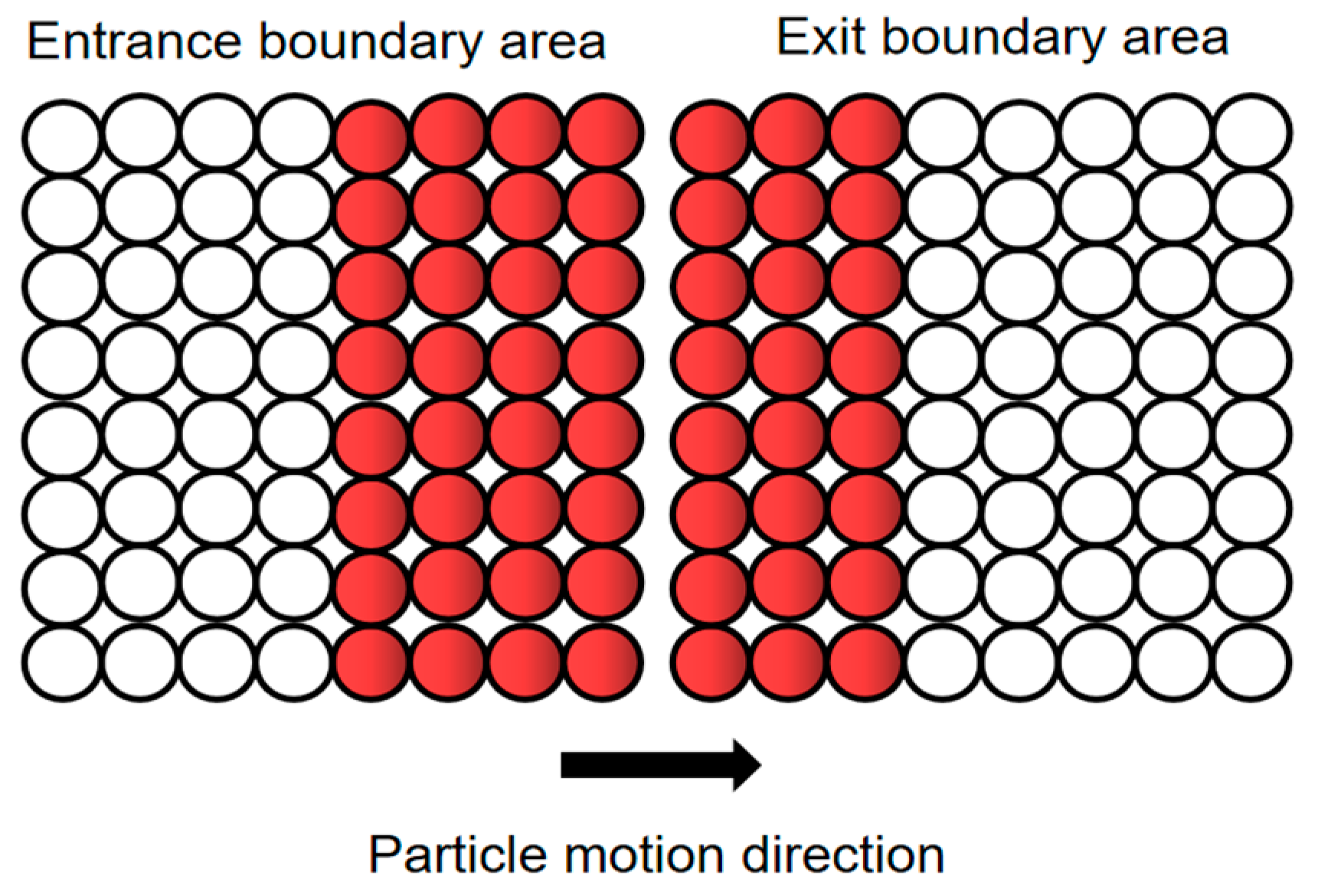
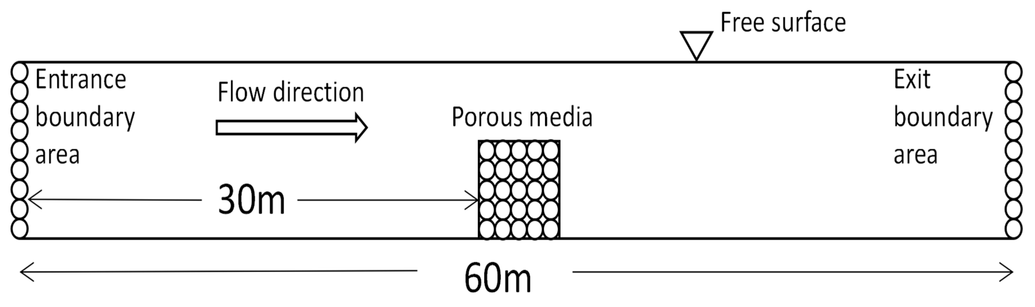
According to previous studies conducted on pore structure logistics field, this paper adopts the boundary of inflow and outflow as displayed in Figure 1 below.
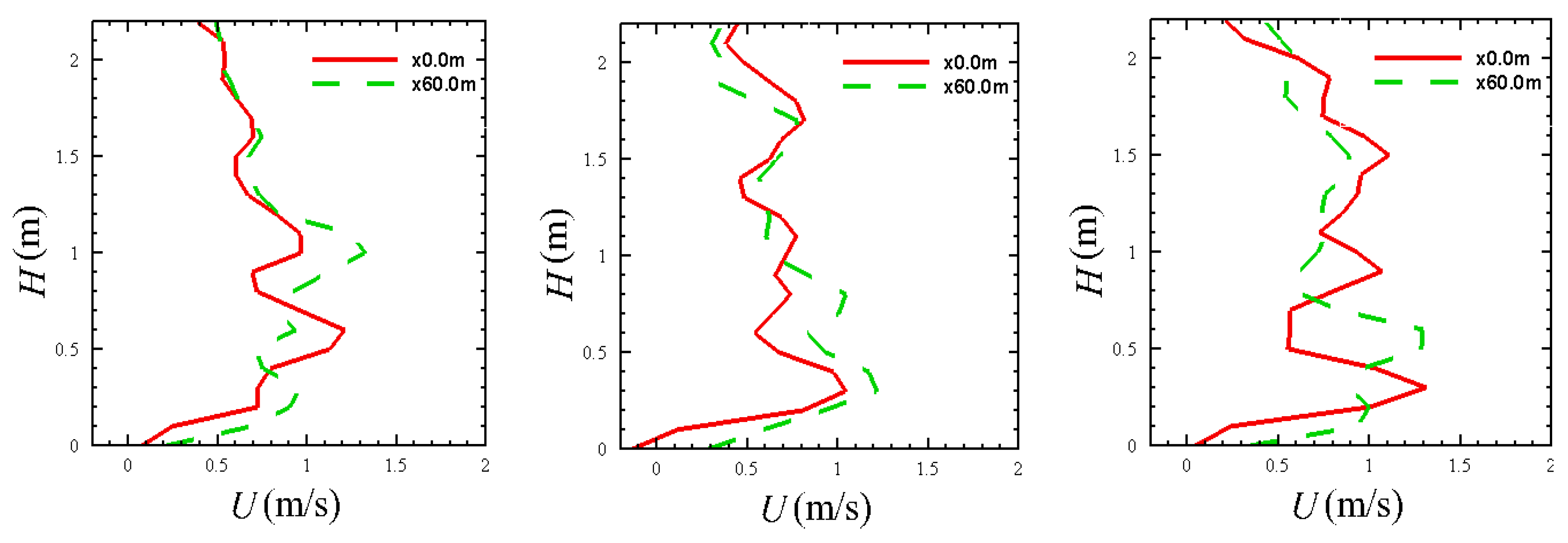
Particles leaving one side of the computational domain move directly through the other side, and particles near the open side boundary interact with particles near the complementary open side boundary. The fluid particles near the left end of the channel can also interact with the fluid particles near the right end in the core affected area. In this sense, the upstream and downstream boundaries can actually be considered as overlapping. In the SPH numerical algorithm, we used the particle linked list to search for neighborhoods through a square grid with a side length of 2*H. Therefore, the fluid particles in the first column of the block located near the upstream boundary can be in contact with the particles in the last column of the block located near the downstream boundary, and vice versa, so the exit boundary flow velocity is also consistent with the inlet boundary flow velocity trend. As a preliminary test to verify this hypothesis, we set the calculation area as 3 m, the inlet flow rate as 0.00936 m3/s, and the particle size D as 0.1 m. In order to further test the performance of our method, three time stages t = 18.0 s, t = 20.0 s, and t = 22.0 s were considered to analyze its inlet and outlet flow rate, respectively. x = 0.0 represents the inlet flow rate distribution curve; x = 60.0 represents the outlet flow rate distribution curve. Analyzing the tests shown in Figure 2, it is possible to notice that the flow distribution of the particles is very similar between inlet (x = 0.0) and outlet (x = 60.0). Furthermore, the velocity ranges from 0 m/s to 1.5 m/s for each time step displayed proving the periodic boundary conditions of the inlet and outlet.
It can also be observed from Figure 2 that the inlet and the exit boundary particles are basically consistent in the horizontal direction despite different time steps considered, confirming that the particles at the exit layer can smoothly enter the inlet across the boundary.
However, if the flow is significantly disturbed before exiting the outlet boundary, the inflow condition will inherit these disturbances and affect the downstream flow. In that case, at least a damping zone is needed downstream the inlet boundary and a numerical calibration is needed to clarify the effectiveness of the damping zone [26,27]. For this study, a damping zone is set at the junction of the exit boundary and the entrance boundary.
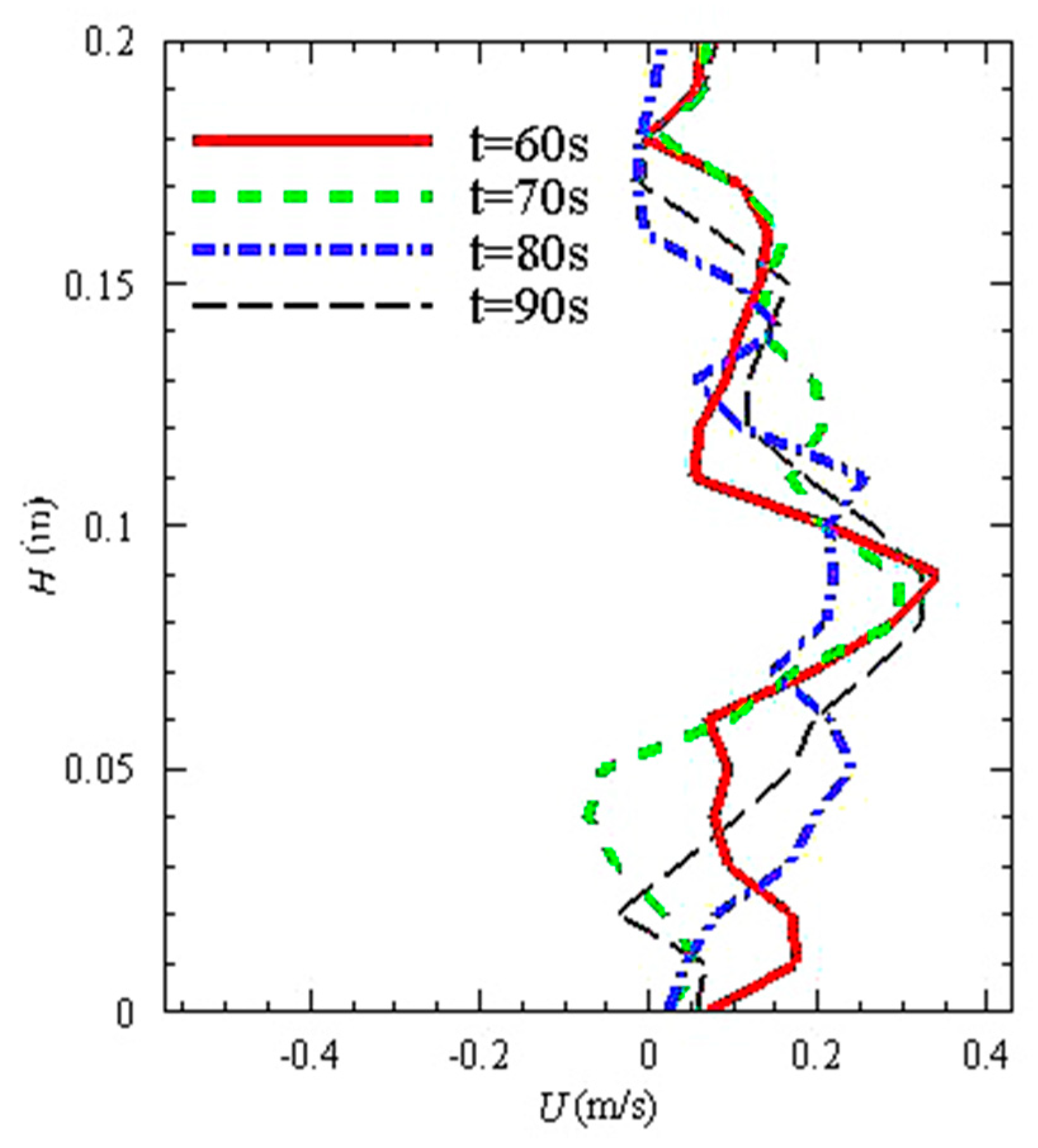
Figure 3 displays the distribution of the velocity of the flow at the exit boundary along the depth of the water after passing through the damping zone. It can be seen that the speed variations remain relatively stable along the depth of the water at different times (t = 60 s; t = 70 s; t = 80 s; t = 90 s), hence the flow velocity at the outlet remains basically identical (the average flow velocity is stable at about 0.13 m/s at all times) as well as the inlet velocity. Under the effect of the periodic boundary, the inlet velocity can be stably maintained at 0.13 m/s so that the flow is significantly disturbed before it departures the exit boundary without affecting the downstream flow. This further validates the effectiveness of the damping region.
For all these reasons, it is possible to confirm the numerical characteristics of the periodic cyclic boundary of the flow.
4. Model Verification
In order for SPH to work in numerical sink simulations, characterizing the correct flow into the outflow boundary is key to achieve a continuous steady flow cycle. In this study, the flow was simulated using periodic boundary conditions and a damping zone. The position and velocity of the particles were firstly initialized, simulating the state of the current at the beginning of the movement. At the same time, during the interaction between the current and the porous media, the flow velocity was considered to change with the variation of the porosity. According to the experiments in the literature, porosity values of 0.349 and 0.475 [7] are the most commonly used and hence have been considered in this work to verify the model adopted.
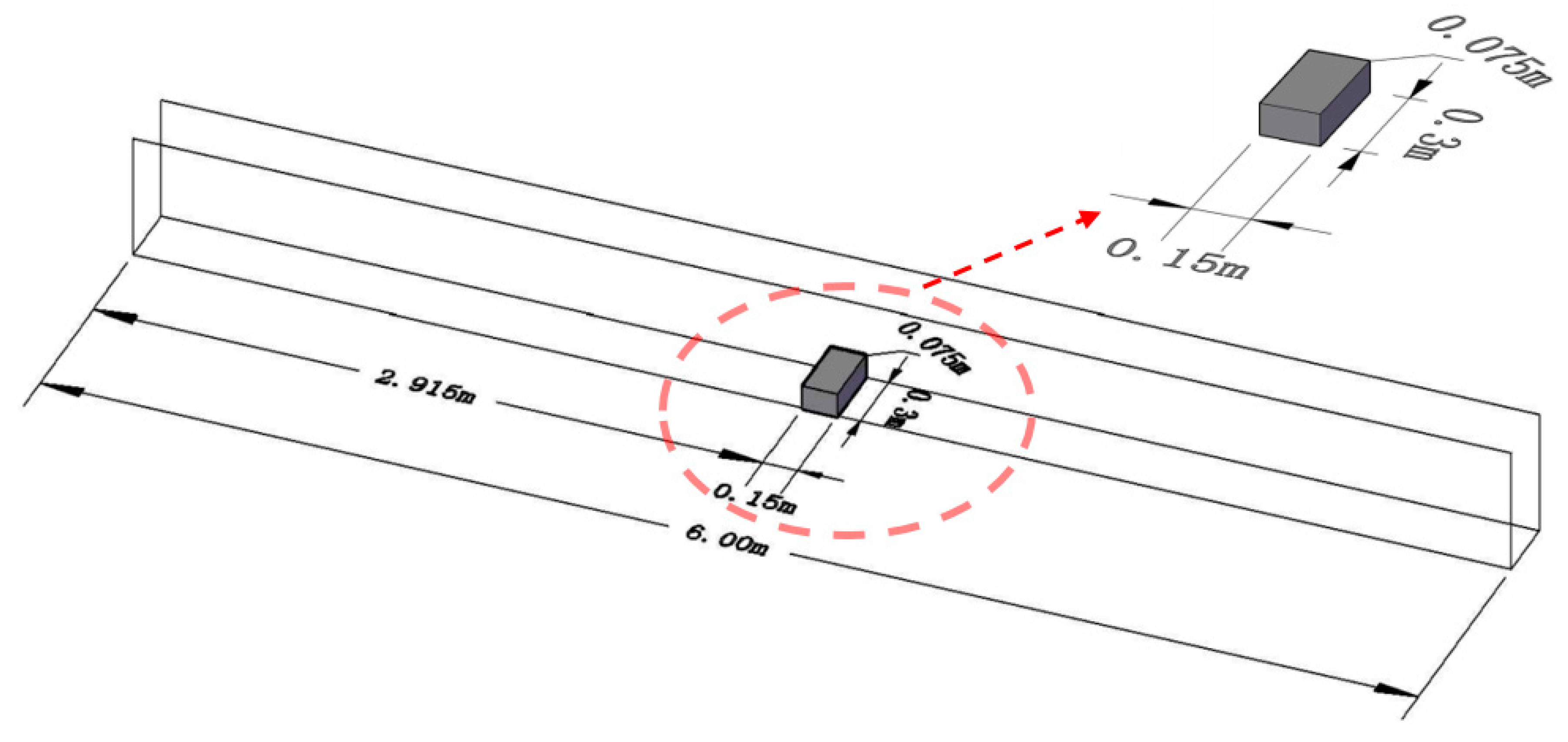
The numerical water tank used for verification is shown in Figure 4 below [7]. The numerical flume has a pore structure placed 2.915 m away from the inlet boundary. The numerical model tank has a length of 6.0 m, an inlet flow rate of 0.13 m/s, a pore structure long 0.15 m and elevated 0.075 m, a sink channel slope of 0.005, and a viscosity of 1.0 × 10⁻⁶ (Pa·s). Finally, the flow field characteristics were simulated at the porosity of 0.349 and 0.475.
The flow fields of velocity vectors for porosity equal to 0.349 (Figure 5a) and 0.475 (Figure 5b) are shown below in Figure 5.
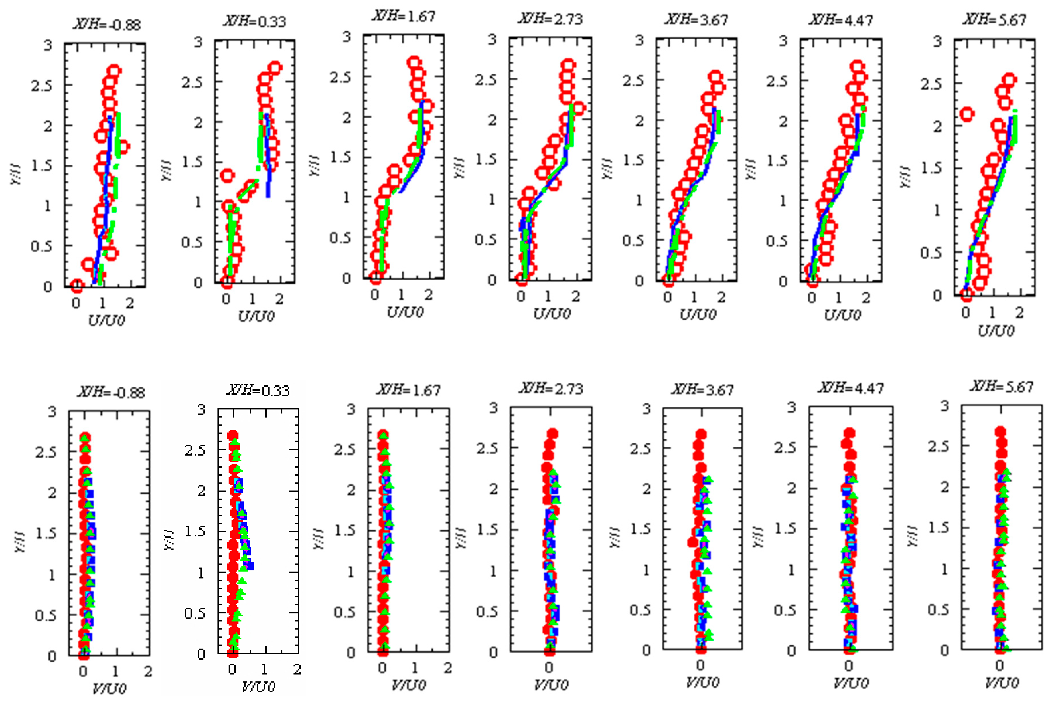
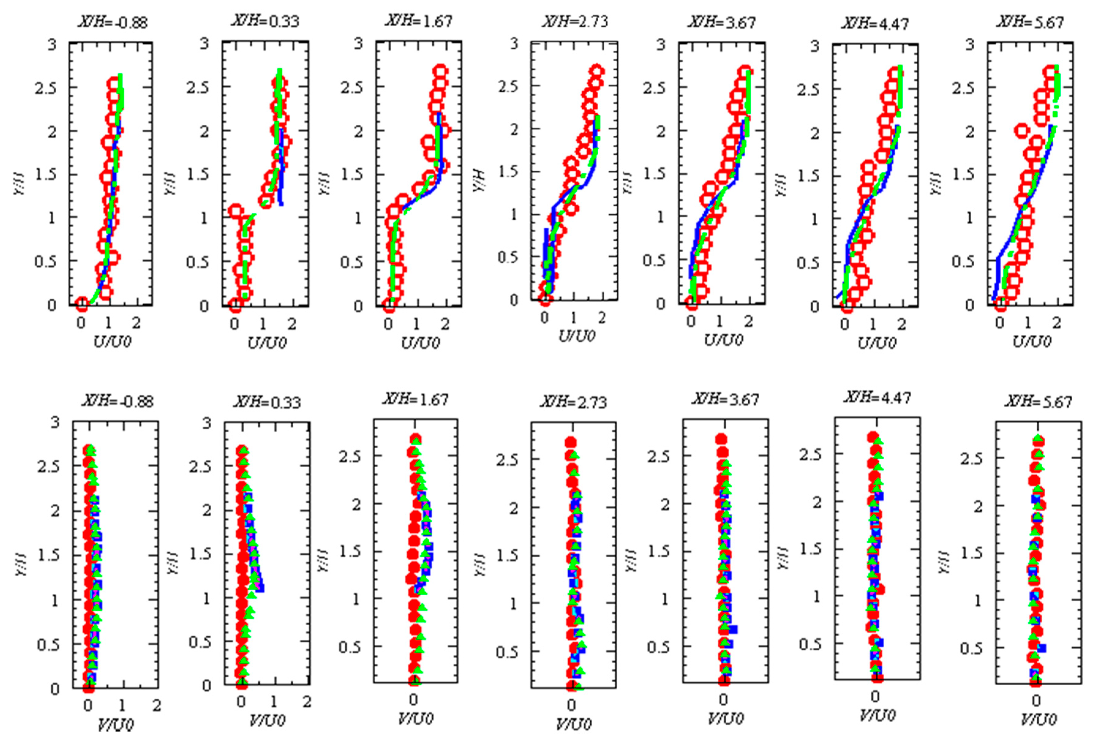
It can be seen from Figure 5 that the flow simulation based on the periodic boundary basically simulates the correct natural movement of the water flow. The internal and external flow fields and back vortex flow fields of the porous media are also visible in Figure 4. The flow field characteristics, the flow velocity U, V, and water depth H were processed dimensionless to verify the flow field velocity distribution characteristics of the porous media at 0.475 and 0.349 and results are shown in Figure 6 and Figure 7, respectively.
The numerical simulation of the longitudinal and vertical velocity distributions at different locations around the porous media fit well (±5–10%) with the velocity curves measured for the experimental experiments. This confirms that the SPH method is feasible for the simulation of the flow field around the porous media and the analysis of the longitudinal and vertical velocity at a porosity of 0.475.
According to the above model verification displayed in Figure 7, it can also be seen that the SPH method can simulate the flow field inside and around the porous media at a porosity of 0.349, and results are consistent with the experiment of the flow field inside and outside the porous media. The model error is between 10% and 15%.
Observing Figure 6 and Figure 7, which show the average flow direction and vertical velocity components at different locations, it is also possible to notice specific features that are worth to be highlighted. At X/H = 0.33, the velocity gradient is large. In the vertical position, the upstream edge of the structure (X/H = 0.33) is 1 < Y/h < 1.5, and the velocity is small. At the downstream edge of the structure (X/H = 1.67), according to its velocity curve, it can be seen that the permeability of porous media is good, and its reverse velocity is small.
X/H = 0.33 indicates that the position is 0.02475 m from the left boundary of the pore structure which is placed at the origin. This location is characterized by the velocity distribution of the flow field when the water flow is coupled with the left boundary of the pore structure. Because this is a periodic boundary and a damping region is added to the flow field, the damping region typically causes some disturbance to the flow field in the initial stage, but the effect of the damping region on the flow field velocity gradually decrease after the particles run for 20 s. It was verified within the model that the deviation has a small effect on the flow field around the pores, and it can be seen that the flow field around the pores is not greatly affected by the damping area.
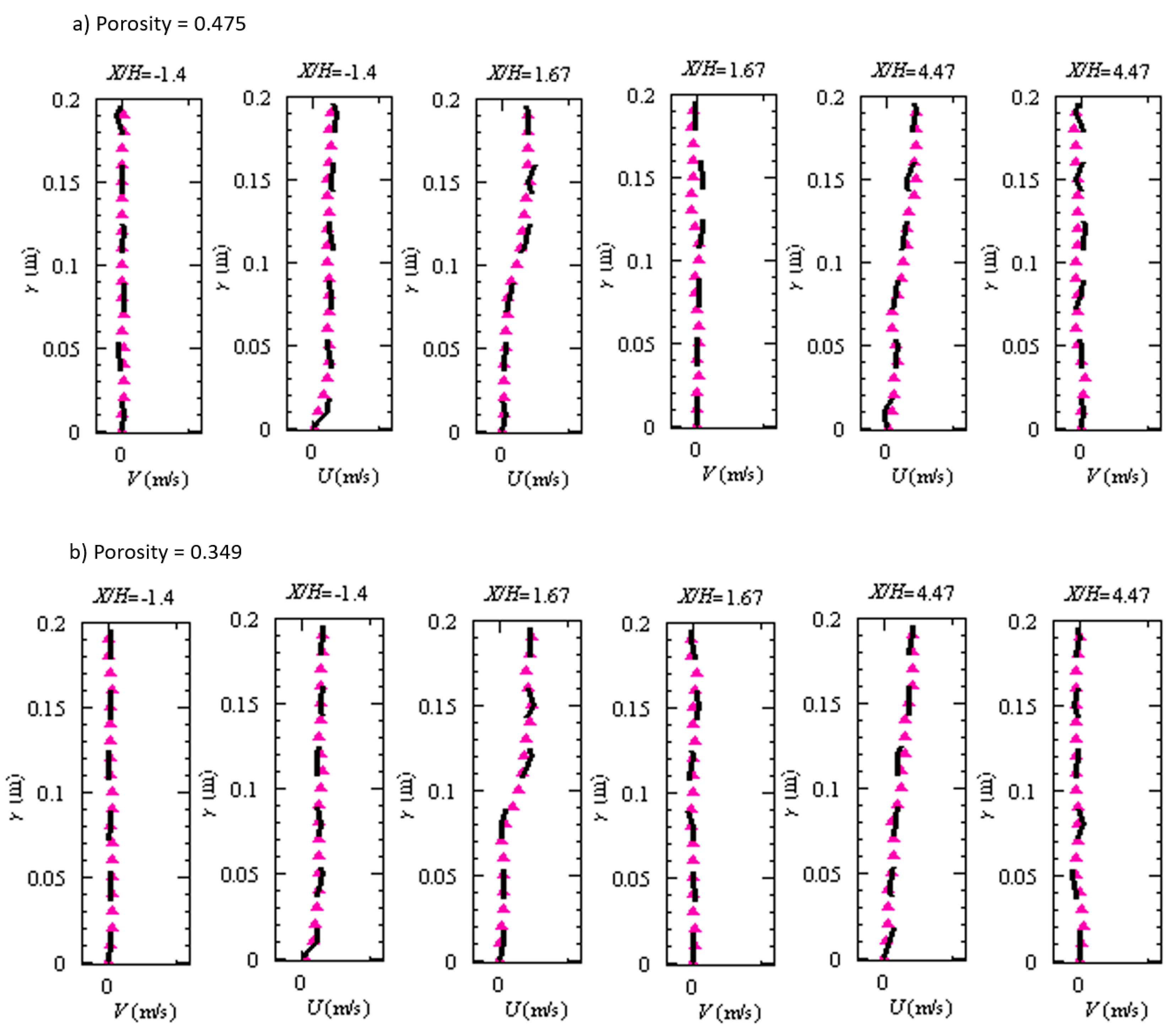
However, in order to ensure that in the oncoming flow field of the pore structure, the flow simulation of the three parts of the pore flow field and the back vortex field of the pore structure have good convergence, the convergence analysis (Figure 8) was completed.
Figure 8 depicts the convergence analysis of the vortex area behind the pore structure and the vortex structure in the oncoming flow area when the porosity is 0.475 and 0.349, respectively. Analyzing Figure 8, it is possible to state that the particles pass through these three areas, and that due to the good convergence and good curve fitting that can be observed, the simulation with different particle sizes still meets the requirements of good convergence.
In practical engineering, the seepage problem of permeable structure will be helpful to the analysis of important engineering structures. It is necessary to study the flow state of fluid in permeable structure. The traditional velocity measurement method is difficult to be used in permeable buildings. Particle image velocimetry (PIV) and particle tracking velocimetry (PTV) are other robust experimental techniques to solve this problem [28,29,30,31,32,33,34,35]. In this study, the Lagrangian particle tracking method is used to measure the velocity distribution along the water depth at different positions.
5. Model Application
According to the model verification previously described in Section 4, it can be confirmed that the numerical simulation method based on SPH simulates appropriately the water flowing on the porous media, thereby it was decided to apply this model to a water tank and a porous media featuring periodic boundaries and a damping zone. The length of the domain is 60 m, at a porosity value is 0.5, particle size is 0.15, pore length, width, and height ranges within 0.6 m and 1.5 m, water depth considered corresponds to 2.4 m, viscosity is 1.0 × 10⁻⁶ (Pa·s), structure coordinates are 30.0, 0.0. The schematic diagram of this configuration is displayed in Figure 9.
5.1. Flow Field Velocity Distribution Diagram of Different Volumes of Porous Media
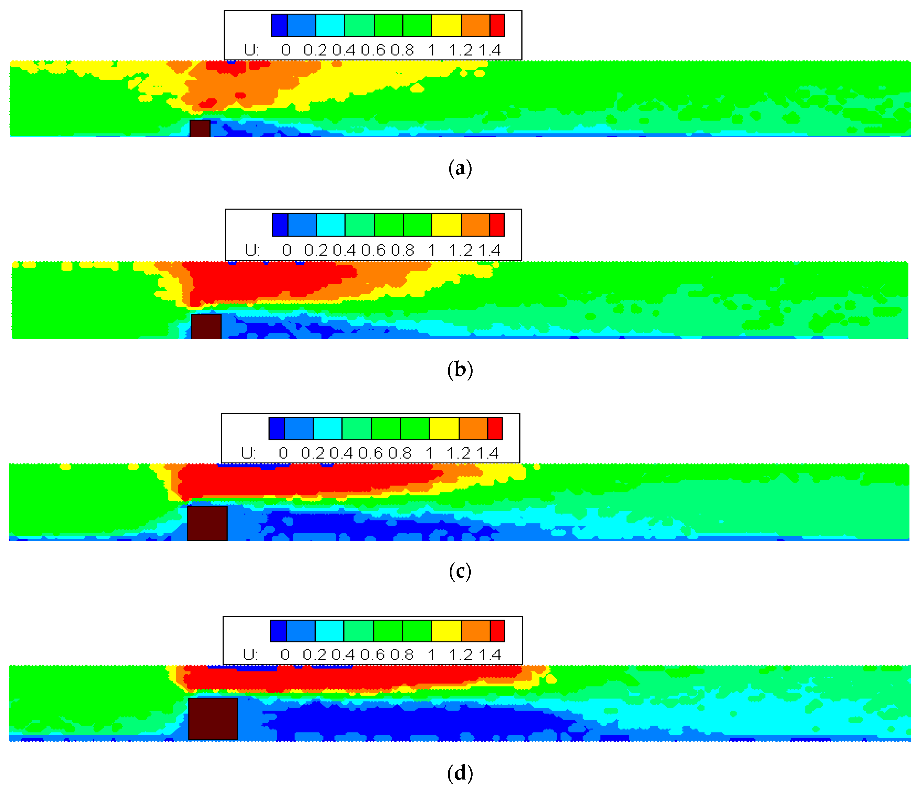
Figure 10 shows the flow field velocity distribution of different volumes of porous media at the porosity of 0.5. According to the flow field displayed below, as the volume of the porous media increases (from top to bottom), the longitudinal flow velocity U of the upper layer of the porous media gradually increases, and the upward-incidence flow region is also expanding, but the enlarged region is not well defined. During the expansion process, the back vortex area expands, and multiple vortex motions are formed. The vortex area increases with the volume of the porous media, and begins to form when the vertical section of the porous media is equal to 1.2 m × 1.2 m. While there is an increase of pore structure volume, the back vortex area expands as well but the eddy strength decreases.
5.2. Analysis of Flow Field Inside and Outside the Porous Media
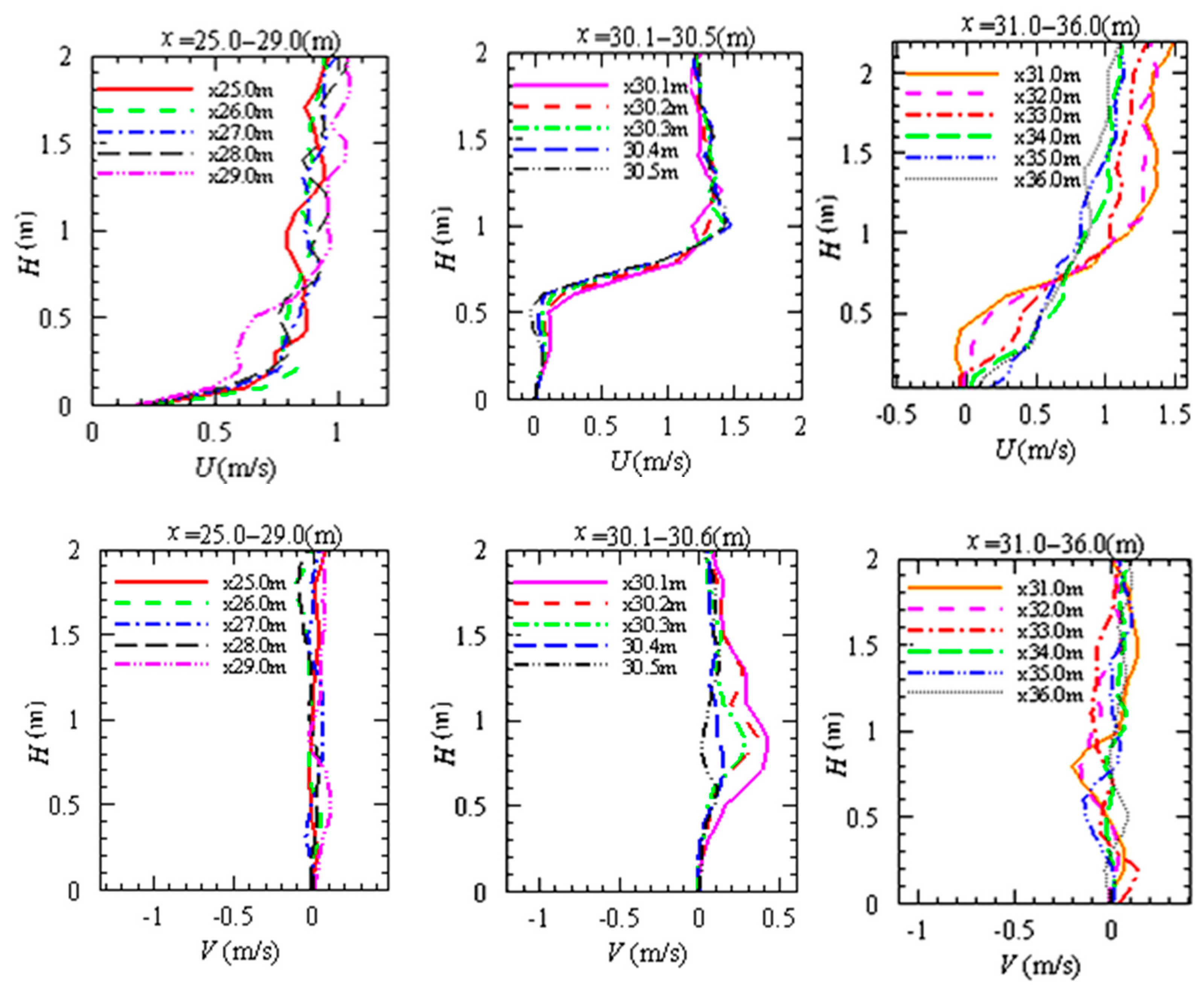
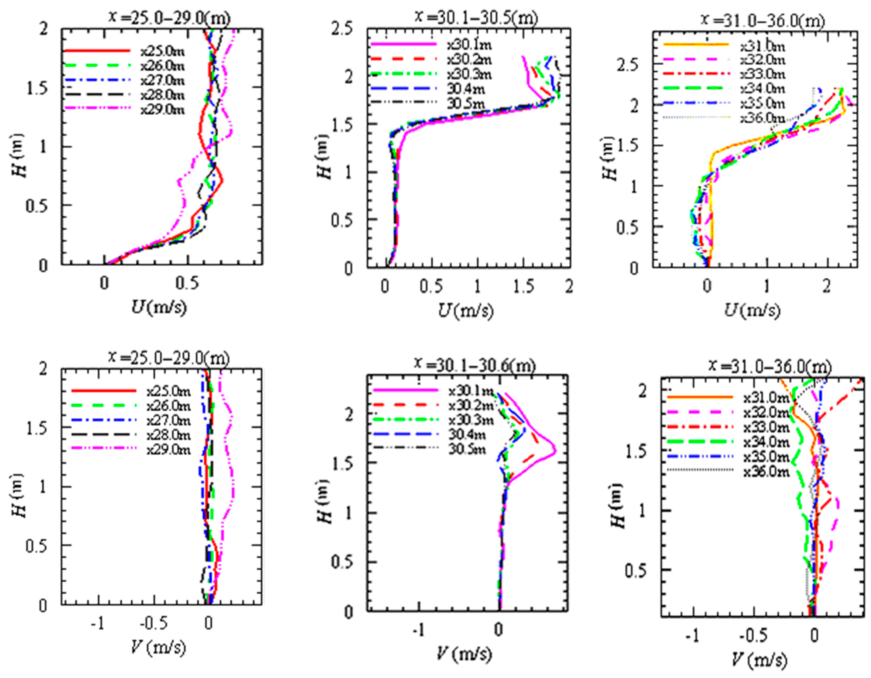
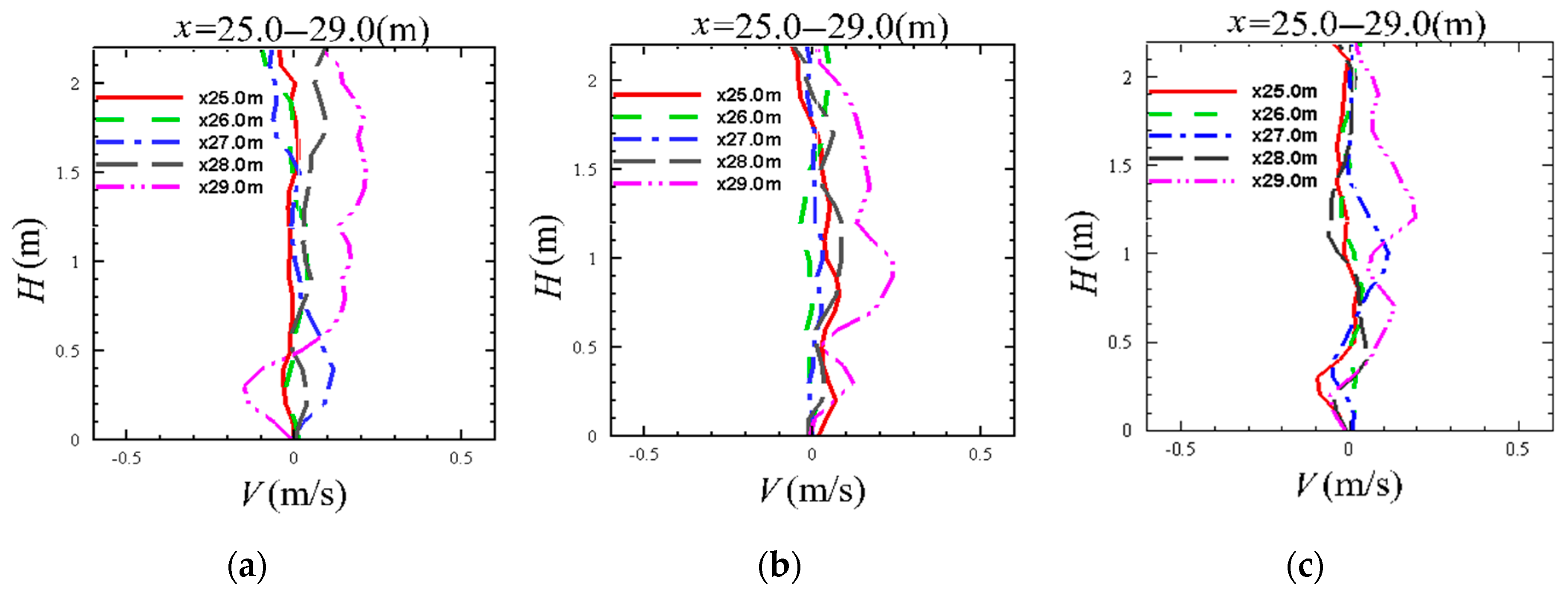
Figure 11 displays the horizontal and vertical velocity of the flow in the upstream area of 0.6 m × 0.6 m pore structure (the area where water flows through the pore structure and the vortex area). In this Figure 11, as well as for Figure 12, Figure 13 and Figure 14, x = 25–29.0 m represents the horizontal coordinate range of the upstream area, x = 30.1–30.5 m represents the horizontal coordinate range of the flow through the pore structure, and x = 31.0–36.0 m represents the horizontal coordinate range of the vortex area.
Moving from x = 0.0 m towards the pore structure (located at 30.0 m) when the distance between the water particles and the pore material becomes smaller, the longitudinal velocity u on the upper side of the pore material increases, as well as the internal velocity of the pore material. The average velocity of this area tends to be stable at about 1 m/s, and the vertical average velocity V ranges between −0.2–0.1 m/s.
When x = 30.1–30.5 m, the water flows through the pore area. Increasing x, at the initial part or the pore structure, the longitudinal velocity u increases from 0.15 m/s to 1.5 m/s, showing the trend of short-term reflux. Therefore, it can be considered that the pore structure of 0.6 m × 0.6 m has an obvious energy dissipation effect, while in the upper water area of the pore structure, the flow velocity shows a slow upward trend and tends to be stable at 1.3 m/s. In the meantime, the vertical average velocity V ranges between −0.2 and 0.4 m/s.
When x = 31.0–36.0 m, this stage is the eddy current area at the back of the pore structure. It can be seen from the change of the back vortex flow field that with the increase of the volume of porous media, there is a turning point at the speed of H (m) = 0.6 m. There are two stages of velocity curves, before and after the turning point, that can be described independently. The first stage represents the velocity curve inside the pore structure, and the second stage corresponds to the velocity curve outside the pore structure. When H is less than the height of pore structure, the velocity of the flow particles increases with the increase of distance from the right boundary of pore structure, with an average velocity of 0.5 m/s; when the water level H is greater than the height of the pore structure, the velocity decreases getting far away from the right boundary of the pore structure, while when x > 30.6 m, and H < 0.6, the velocity of the flow particles on the right boundary of pore structure decreases with the increase of distance from the right boundary of the pore structure. When x = 36.0 m, the flow particle velocity reaches the peak of 1.3 m/s. For this scenario, the vertical average velocity V is between −0.2 and 0.1 m/s.
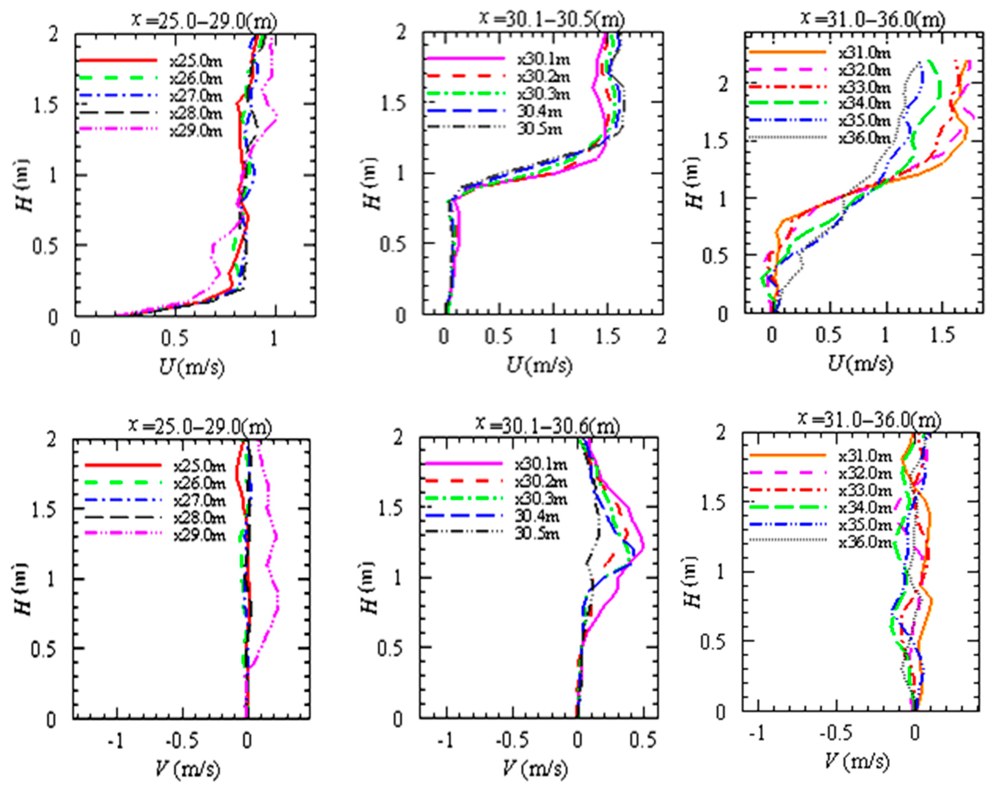
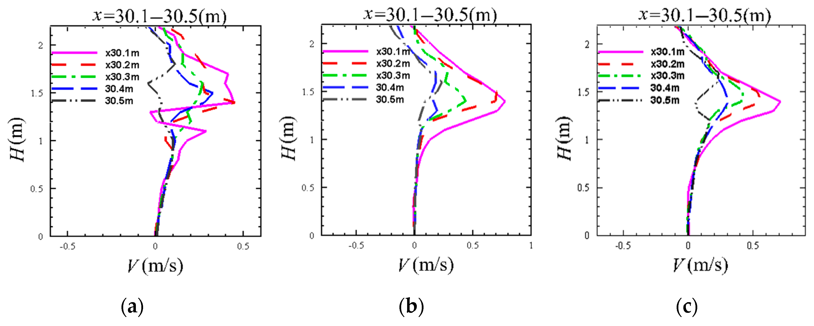
Figure 12 displays the horizontal and vertical velocity of the flow in the upstream area of 0.9 m × 0.9 m pore structure (the area where water flows through the pore structure and the vortex area).
When x = 25–29.0 m, with the increase of x, that is, when the distance between water particles and pore structure becomes smaller, the particle flow velocity in the upstream area of pore structure slightly decreases when the longitudinal velocity u on the upper side of pore structure is 0.6 m higher than the one recorded on the side, while the internal velocity growth of the pore structure is still almost negligible. The pore structure is more stable when the overall average velocity is 0.6 m higher than the side length, and the average up-flow velocity tends to be stable when it is close to 1 m/s, while the vertical average velocity V ranges between −0.2 and 0.1 m/s. With the increase of x, the longitudinal velocity u on the upper side of the porous material increases slightly, and the decrease observed on the left side is equal to the height of the porous material. The total velocity of the upwelling increases gradually, and tends to be stable near 0.9 m/s. The vertical velocity of the upwelling area remains almost stable at 0 m/s.
When x = 30.1–30.5 m, water flows through the pore structure area. With the increase of x, the longitudinal velocity u of the fluid in the pore structure decreases gradually, but this phenomenon is not significant, and the reflux trend weakens. Therefore, it can be judged that the energy dissipation effect of the pore structure is slightly stronger when the side length is 0.9 m than when the side length is 0.6 m, while in the upper water area of the pore structure, the flow velocity shows a slow upward trend. When the height h is constant, the flow velocity decreases with the increase of x, and the overall flow velocity still increases with the increase of H.
When x = 31.0–36.0 m, an eddy current area at the back of pore structure can be noticed. It can be seen from the change of the back vortex flow field that there is a turning point in the velocity distribution curve at H = 1.5 m. When H is less than the height of porous material, the velocity increases with the increase of x, and the average velocity is 0.25 m/s; when h is greater than the height of porous material, the velocity decreases with the increase of x, and reaches 1.7 m/s at x = 36.0 m, and the back vortex strength decreases with the increase of the distance from the hole. The vertical velocity is relatively stable, in the range of −0.15 and 0.1 m/s.
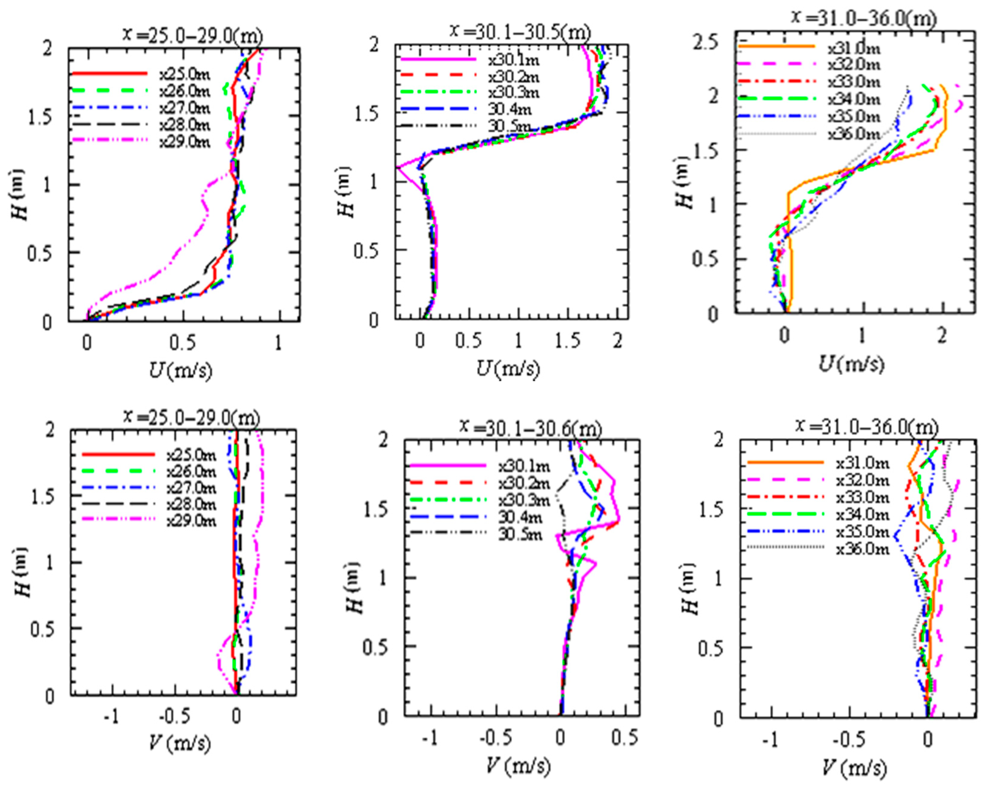
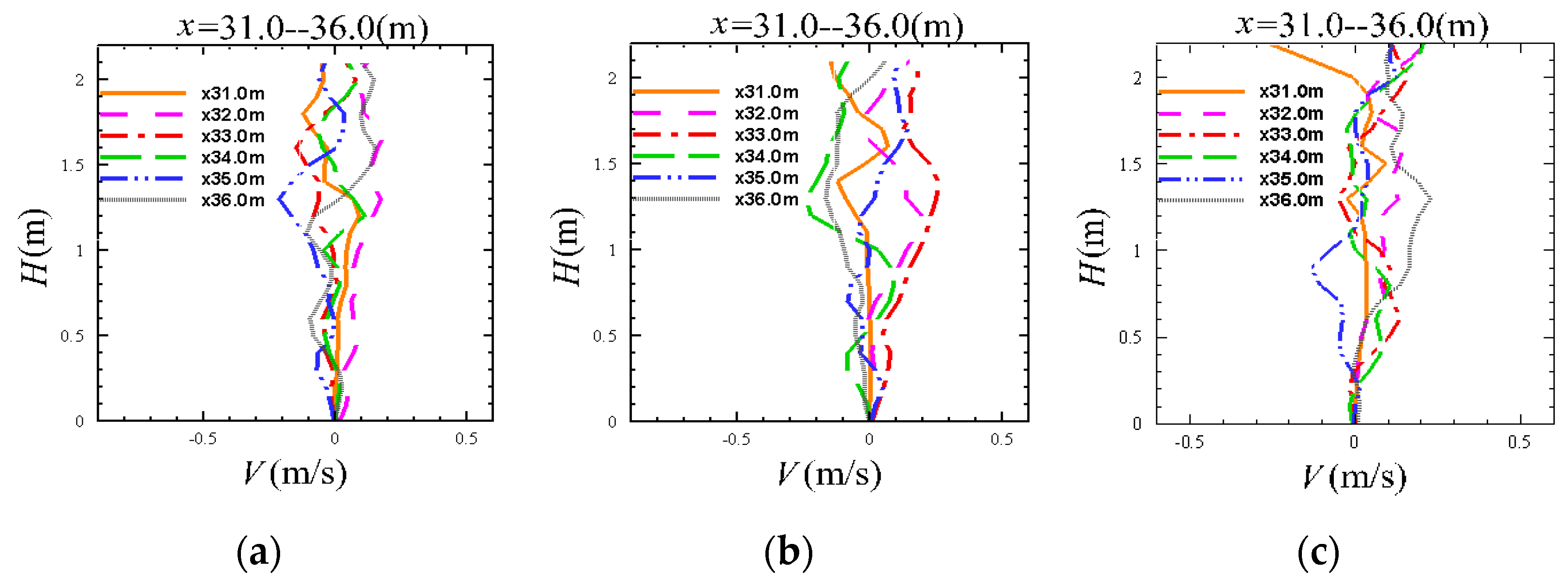
Figure 13 displays the horizontal and vertical velocity of the flow in the upstream area of 1.2 m × 1.2 m pore structure (the area where water flows through the pore structure and the vortex area). When x = 25–29.0 m, with the increase of x, the particle velocity in the upstream area of the pore structure decreases slightly when the longitudinal velocity u on the upper side of the pore structure is 0.9 m longer than that on the side, and the average velocity of upwelling tends to be stable at the place close to 0.8 m/s, and the vertical average velocity V is between −0.15–0.1 m/s. When x = 30.1–30.5 m, water flows through the pore area.
With the increase of x, the longitudinal velocity U of the fluid in the pore structure is gradually stable at 0.1 m/s, and the reflux trend is not strong. It can be seen that for 1.2 m × 1.2 m porous material, the energy dissipation effect of porous material is also stronger than before. When x = 31.0–36.0 m, when H is greater than the hole height, the velocity decreases with the increase of x, and the velocity at the right boundary of the pore structure decreases with the increase of the distance from the right boundary of the hole to 2.0 m/s. The back vortex intensity also decreases with the increase of x. The vertical velocity is relatively stable, in the range of −0.20 and 0.35 m/s.
Finally, Figure 14 displays the horizontal and vertical velocity of the flow in the upstream area of 1.5 m × 1.5 m pore structure (the area where water flows through the pore structure and the vortex area). When x = 25–29.0 m, the overall velocity of the upwelling increases gradually, and tends to be stable (approximately 0.75 m/s), while the vertical velocity ranges between −0.2 and 0.2 m/s.
When x = 30.1–30.5 m, water flows through the pore area. With the increase of x, the longitudinal velocity u of the fluid in the pore structure tends to 0, and the reflux trend is not noticeable. It can be concluded that the hole has obvious energy dissipation effect on the hole of 1.5 m × 1.5 m, while in the upper water area of the hole, the velocity keeps rising slowly. With the increase of distance, the water content of the upper part of the pore structure shows a slowly rising trend, the vertical velocity increases at the same time. When x = 31.0–36.0 m, when h is less than the height of porous material, the flow velocity increases with the increase of the right boundary distance of porous material, and the average flow velocity is approximately 0.02 m/s; when h is greater than the height of porous material, the flow velocity decreases with the increase of the right boundary distance of porous material, and the flow velocity at the right boundary of porous material reaches 2.2 m/s, and the back vortex strength decreases with the increase of the distance from the hole. The vertical velocity is relatively stable, in the range between −0.35 and 0.35 m/s.
In summary, based on the changes of up-flow field tested, it can be stated that by increasing the pore volume, the up-flow velocity typically decreases and the energy dissipation becomes higher, but changes associated with the vertical velocity are not significant with the change of volume for the pore structure. Focusing on the change of the flow field inside and outside the hole it is possible to confirm that the internal velocity of the pore is mainly in the range of 0 and 0.2 m/s. With the increase of the porous media’ volume, the internal velocity difference of the pore decreases gradually, while the particle velocity directly above the pore structure increases with the increase of the pore volume, and the velocity difference of the upper layer flow also gradually increases.
Furthermore, it can be seen from the change of the back vortex flow field that, with the increase of the volume of porous media, there are inflexion points at H (m) = 0.6, 0.9, 1.2 and 1.5 for the four groups of horizontal velocity, respectively, thus forming multiple velocity curves before and after the inflexion point. When H is less than the height of the hole, the flow velocity increases with the increase of x, however when H is greater than the height of the hole, the flow velocity increases with the increase of x. The intensity of the back vortex also decreases with the increase of x. From the change of vertical velocity, it can be observed that the velocity basically varies from −0.5 m/s to 0.5 m/s.
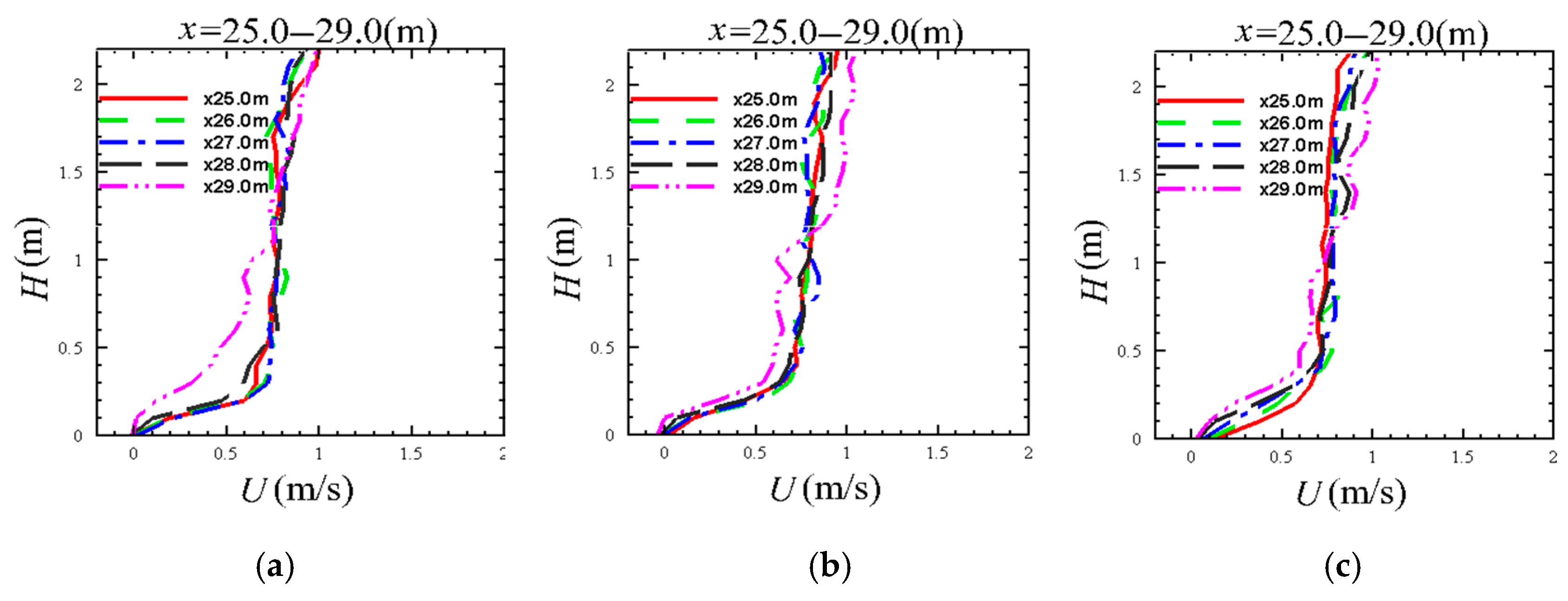
5.3. Longitudinal and Vertical Flow Field Distribution under Different Porosity
Porosity is also an important factor influencing the characteristics of the flow field in the porous media [36]. Therefore, the pore size was 1.2 × 1.2 (m), and the oncoming flow and reflux vortices were analyzed for porosity values of 0.5, 0.25 and 0.125, respectively. The velocity distribution and the flow field along the water depth were analyzed for each porosity investigated.
Figure 15 displays the flow field in the upstream area of pore structure under different porosities 0.5, 0.25, and 0.125 for x = 25.0–29.0. As the porosity decreases, it can be seen that the longitudinal velocity curve of the upstream flow tends to be gradually stable.
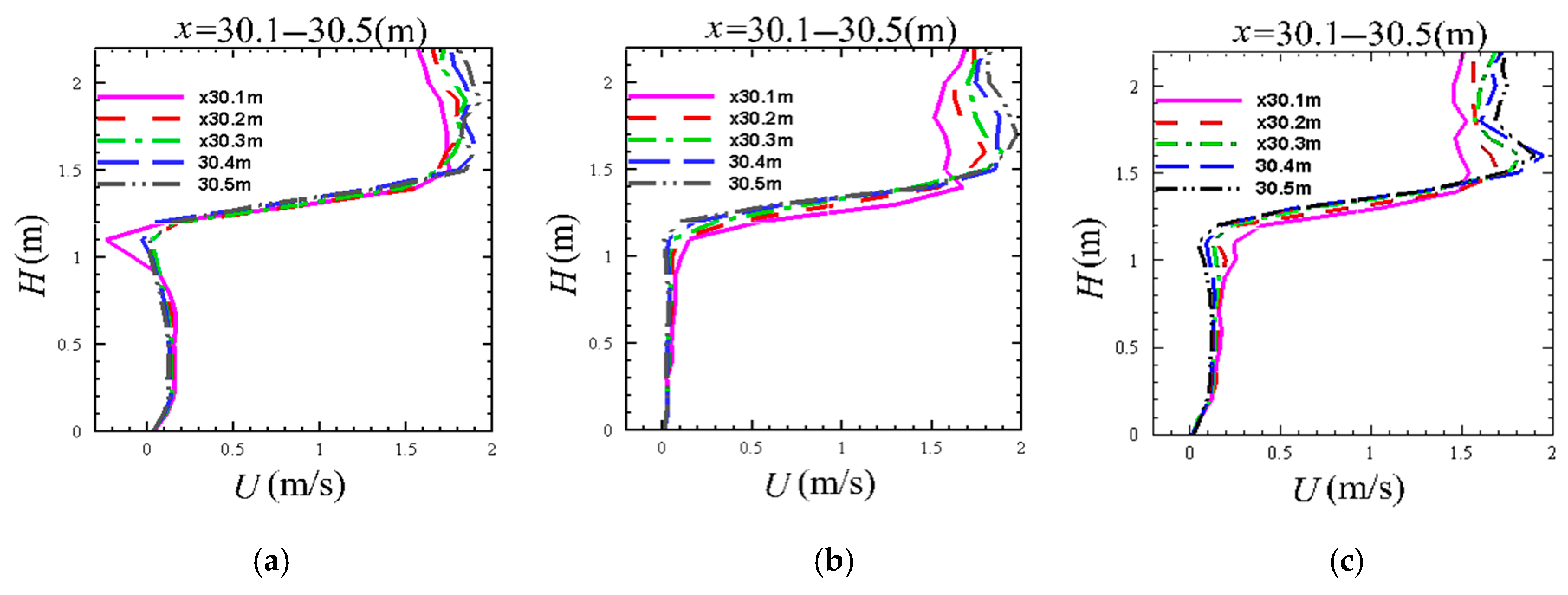
Figure 16 shows the flow field when the water flows through the pore structure under different porosities 0.5, 0.25 and 0.125 for x = 30.1–30.5. The longitudinal velocity difference of the internal flow field of the pore structure increases with the decrease of porosity.
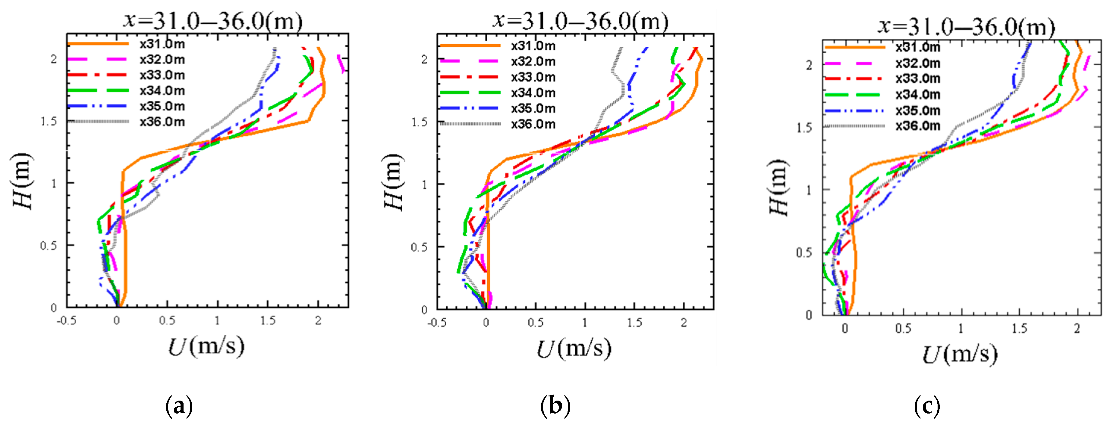
Figure 17 presents the flow field in the back vortex region with different porosities 0.5, 0.25 and 0.125 for x = 31.0–36.0. With the decrease of porosity, the flow rate changes are not significant, but the back vortex region increases slightly, and the flow rate at the inflection point also initially increases but later decreases in combination with the increase of porosity. When the porosity is 0.25, the particle longitudinal velocity at the inflection point is the maximum calculated.
Figure 18 displays the vertical velocity distribution of the flow field in the upstream area of the pore structure under different porosities 0.5, 0.25, and 0.125 for x = 25.0–29.0. With the gradual decrease of porosity, it can be seen that the vertical velocity difference of each position of the upstream flow is gradually reduced.
Figure 19 shows the vertical velocity distribution of the flow field inside and directly above the pore structure under different porosities 0.5, 0.25, and 0.125 for x = 30.1–30.5. With the gradual decrease of porosity, it can be seen that in the fluid solid interface area, the change of horizontal velocity becomes more evident, and the velocity reduces.
Figure 20 presents the vertical velocity distribution of the back vortex flow field under different porosities 0.5, 0.25 and 0.125 for x = 31.0–36.0. As the porosity decreases gradually, it can be seen that when the height H is constant, the vertical velocity difference at each position is characterized by a gradually increasing trend.
In summary, it can be seen from Figure 15, Figure 16, Figure 17, Figure 18, Figure 19 and Figure 20 that as the porosity increases, the longitudinal flow velocity of the oncoming flow slightly changes, but the overall change is not significant, plus the longitudinal flow velocity of the back vortex decreases. Considering the vertical flow velocity of the upstream area, despite the increase of porosity, this parameter remains within the range between −0.2 m/s and 0.2 m/s, and the vertical flow velocity through the porous media decreases with the increase of porosity. From the vertical flow velocity of the back vortex, as the porosity increases, the vertical flow velocity tends to decrease slightly overall.
Due to the infiltration of the water, the permeable structure has a significant impact on its discharge capacity [37]. It can be seen from the horizontal and vertical comparison of the flow field in Figure 16 that with the increase of porosity, the flow resistance decreases. The distribution of longitudinal velocity of porous material changes in the upper layer of porous material.
The maximum turbulence intensity near the surface and behind the structure increases proportional to the porosity [38] at the same downstream position.
5.4. Convergence Verification of Pore Logistics Field Model
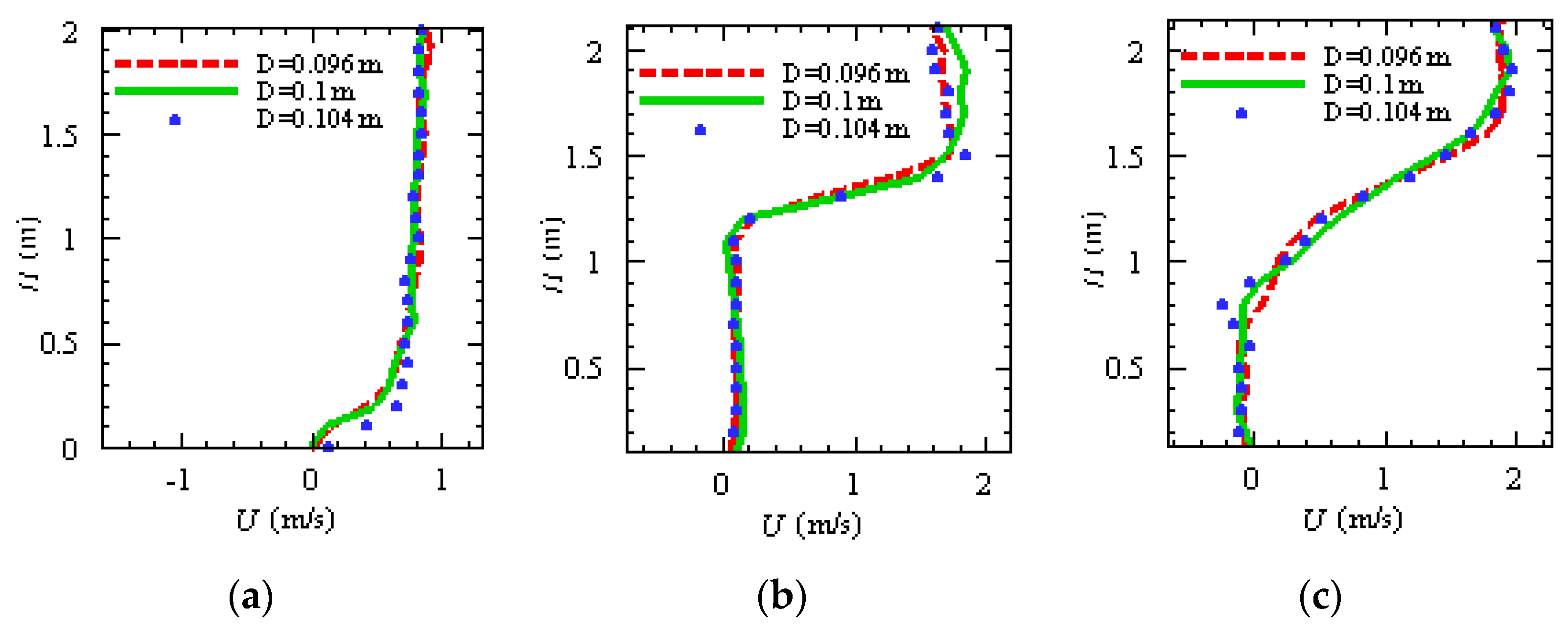
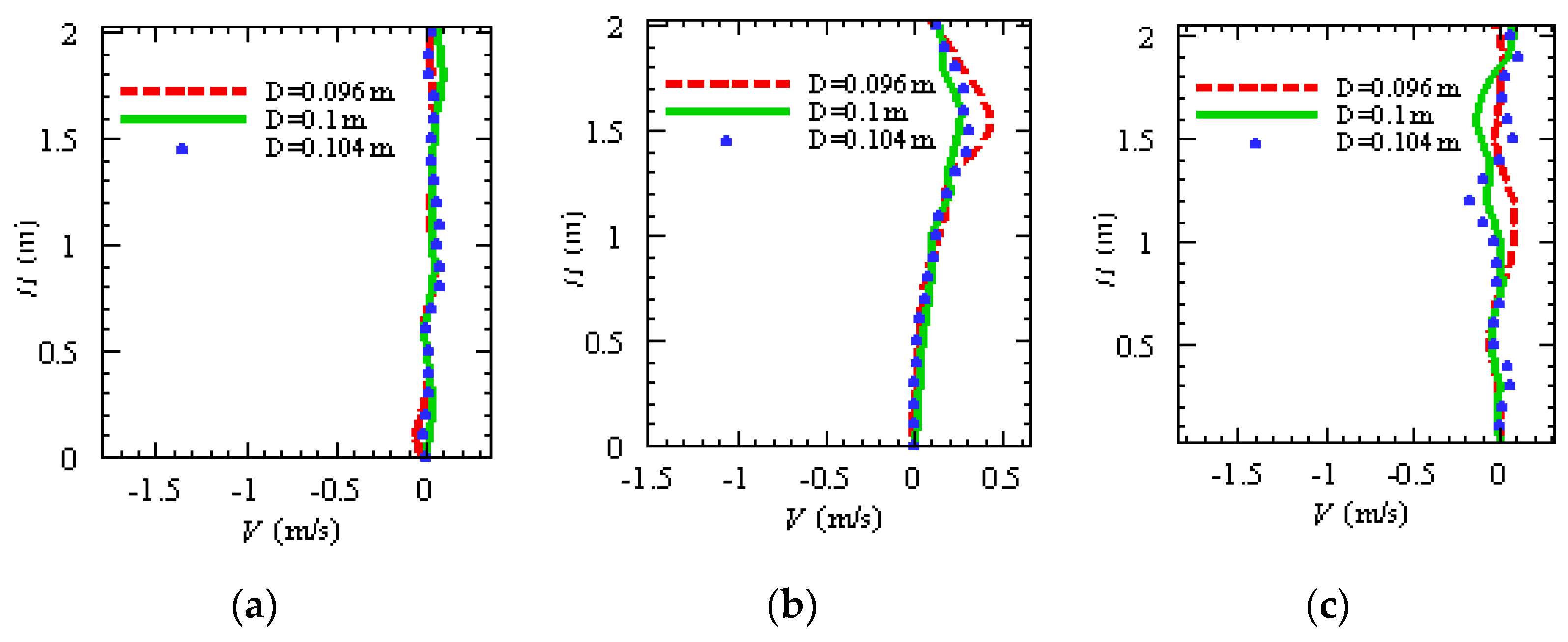
In order to verify the convergence of the SPH in the numerical model, the flow field characteristics of each section previously investigated were analyzed by applying multiple particle size distributions [8]. Up-flow area, pore flow area, back vortex area, and the horizontal and vertical velocity distribution along the depth were calculated with the particle size D of 0.096 m, 0.01 m, and 0.104 m as shown in Figure 21 and Figure 22 to verify convergence, at the selected positions x = 28.0 m, 30.3 m, 33 m.
It was previously noticed that when the height of the pores is 1.2 m, the flow direction is opposite to the others when D = 0.096. This elevation corresponds to the upper flow area of the pore structure and justify the presence of turbulence as shown in the graph. However, results displayed in Figure 21 and Figure 22 show that the velocity distributions of the internal and external flow fields formed by the oncoming flow field, the back vortex flow field and the water flow through the porous media are consistent despite different particle spacing and the error range is between 10% and 15%, hence providing an acceptable grade of convergence.
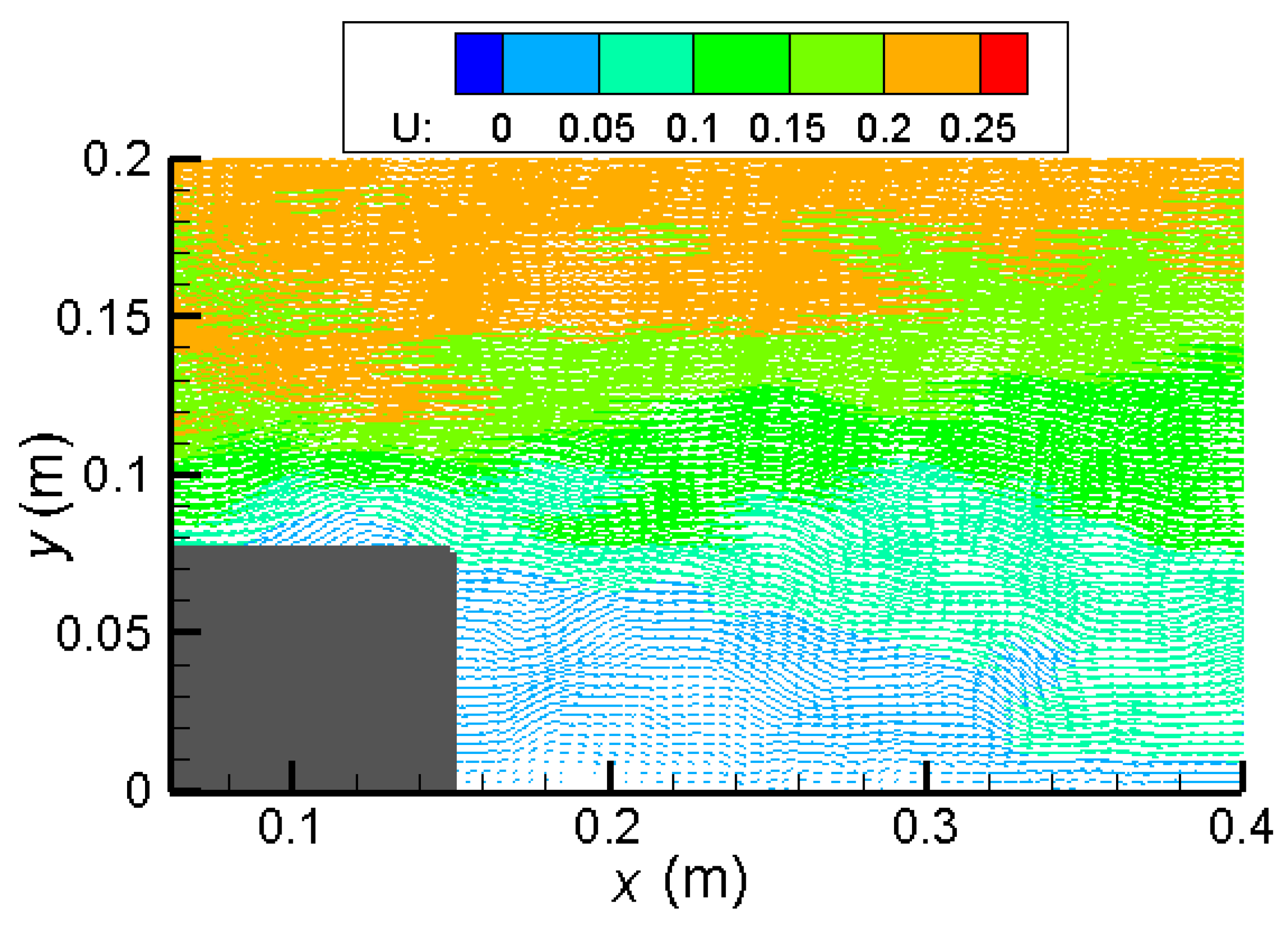
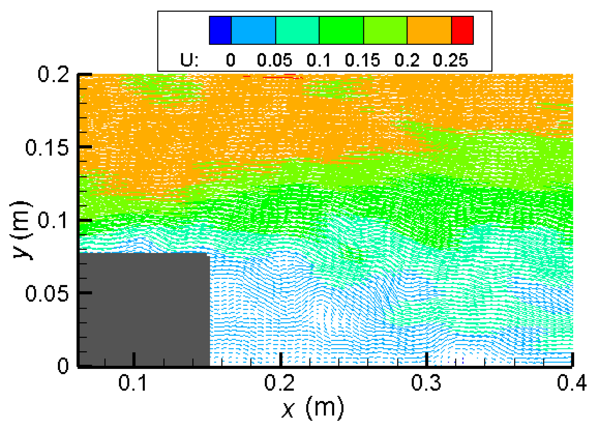
Finally, Figure 23 and Figure 24 show the back vortex field of the pore structure when the porosity is 0.349 and 0.475, respectively.
It can be seen from the flow field distribution diagrams in Figure 23 and Figure 24 that the energy in the vicinity of the pore structure presents a dissipative trend and shows different vorticities under different porosities. When the porosity is 0.475, the energy dissipation in the vicinity of the pore structure is weak, the vortex flow pattern is more noticeable and multiple vortex flow patterns are formed on the back of the pore structure. However, when the porosity is 0.349, the energy dissipation near the pore structure is relatively strong, and the intensity of the vortex flow is relatively weak.
To enable academic colleagues to replicate the presented numerical data and have a better estimation of the numerical capabilities of the numerical method, details about the total number of particles used, the particle size, the physical simulation times plus the CPU time and the CPU cores used are displayed and summarized in Table 1 for all the configurations tested (D = 0.0104 m, D = 0.01 m, D = 0.096 m, D = 0.1 m, and D = 0.104 m).
6. Conclusions
Nowadays, a variety of man-made structures such as submerged breakwaters, fishing reefs, outfall protections, armor layers, rubble-mound or berm breakwaters, built of gravel or artificial units, can be found in coastal areas worldwide for multiple purposes (e.g., coastal flooding protection, coastal erosion protection). All these structures are characterized by the fact that either some of their layers or their full structure are porous, hence they are permeable to flows induced by waves and currents. Therefore, the hydrodynamics, the stability and performance of these structures are dependent on the characteristics of the waves and their interaction with permeable material and it is crucial to provide mathematical formulations to model these features and the role played by the porous material considering its geometry, its location, and its characteristics (which could influence the wave propagation, diffusion, overtopping, and the consequent turbulence generated).
This paper enabled the calibration and validation of a SPH model utilized to characterize the influence of porous media on flow propagation and outcomes can be summarized as follows:
1. Based on the analysis of the area upstream the porous media, the longitudinal flow velocity of the ascending flow decreases slightly with the increase of the volume of the pore structure;
2. Based on the analysis of the internal and external flow fields of the porous media, the internal flow velocity of the porous media for the configurations tested is in the range of 0–0.2 m/s. It was possible to notice that with the increase of the volume of the porous media, the flow velocity of the upper layer of the porous media firstly tends to accelerate and then stabilizes. The longitudinal flow velocity of the upper layer of the flow increases with the increase of water depth, while the vertical velocity fluctuates sharply at the fluid-solid boundary;
3. Based on the back vortex analysis, there is an inflection point in the flow velocity distribution of the upper and lower layers of the porous media. As the distance from the porous media increases, the flow velocity increases, so that the velocity distribution curve of the back vortex flow forms different concavities and convexities before and after the porous media, and as the pore volume gradually increases, a plurality of vortices are formed on the backflow surface. With the rotary motion, the area of the back vortex increases as the volume of the pore increases, but the strength decreases as the volume increases.
4. Overall, with the increase of porosity, the longitudinal flow and back vortex flow slightly decrease in the vertical direction, and the SPH-based model calculation has good convergence (error between experimental and numerical results within 10%).
Author Contributions
Conceptualization, Q.G.; methodology, S.W. and Q.G.; software, S.W. and Q.G.; validation, S.W. and Q.G. and M.R.; formal analysis, S.W. and Q.G.; investigation, S.W., Q.G. and M.R.; resources, S.W. and Q.G.; data curation, S.W., Q.G. and M.R.; writing—original draft preparation, S.W., Q.G. and M.R.; writing—review and editing, S.W., Q.G. and M.R.; visualization, S.W. and Q.G.; supervision, Q.G. and M.R.; project administration, Q.G.; funding acquisition, Q.G. All authors have read and agreed to the published version of the manuscript.
Funding
This research was funded by Zhejiang Province Natural Science Foundation, grant number LQ16E090001, the National Natural Science Foundation of China, grant number 51509134.
Acknowledgments
The author is very grateful to Ningbo University, the National Natural Science Foundation of China and the Natural Science Foundation of Zhejiang Province. All authors are very grateful to Dr Songdong Shao for his constructive comments and continuous inspiration to complete this work.
Conflicts of Interest
The authors declare no conflict of interest.
References
- Espinoza-Andaluz, M.; Velasco-Galarza, V.; Romero-Vera, A. On hydraulic tortuosity variations due to morphological considerations in 2D porous media by using the Lattice Boltzmann method. Math. Comput. Simul. 2020, 169, 74–87. [Google Scholar] [CrossRef]
- Akbari, H. Modified moving particle method for modeling wave interaction with multi layered porous structures. Coast. Eng. 2014, 89, 1–19. [Google Scholar] [CrossRef]
- Houreh, N.B.; Shokouhmand, H.; Afshari, E. Effect of inserting obstacles in flow field on a membrane humidifier performance for PEMFC application: A CFD model. Int. J. Hydrog. Energy 2019, 44, 30420–30439. [Google Scholar] [CrossRef]
- Mei, T.-L.; Zhang, T.; Candries, M.; Lataire, E.; Zou, Z.-J. Comparative study on ship motions in waves based on two time domain boundary element methods. Eng. Anal. Bound. Elem. 2020, 111, 9–21. [Google Scholar] [CrossRef]
- Basser, H.; Rudman, M.; Daly, E. SPH modelling of multi-fluid lock-exchange over and within porous media. Adv. Water Resour. 2017, 108, 15–28. [Google Scholar] [CrossRef]
- Aganetti, R.; Lamorlette, A.; Thorpe, G.R. The relationship between external and internal flow in a porous body using the penalisation method. Int. J. Heat Fluid Flow 2017, 66, 185–196. [Google Scholar] [CrossRef]
- Chan, H.C.; Leu, J.M.; Lai, C.J. Velocity and turbulence field around permeable structure:Comparisons between laboratory and numerical experiments. J. Hydraul. Res. 2007, 45, 216–226. [Google Scholar] [CrossRef]
- Gui, Q.; Dong, P.; Shao, S.; Chen, Y. Incompressible SPH simulation of wave interaction with porous structure. Ocean Eng. 2015, 110, 126–139. [Google Scholar] [CrossRef]
- Khayyer, A.; Gotoh, H.; Shimizu, Y.; Gotoh, K.; Falahaty, H.; Shao, S. Development of a projection-based SPH method for numerical wave flume with porous media of variable porosity. Coast. Eng. 2018, 140, 1–22. [Google Scholar] [CrossRef]
- Vanneste, D.; Troch, P. 2D numerical simulation of large-scale physical model tests of wave interaction with a rubble-mound breakwater. Coast. Eng. 2015, 103, 22–41. [Google Scholar] [CrossRef]
- Shao, S. Incompressible SPH flow model for wave interactions with porous media. Coast. Eng. 2010, 57, 304–316. [Google Scholar] [CrossRef]
- Gnanasekaran, B.; Liu, G.-R.; Fu, Y.; Wang, G.; Niu, W.; Lin, T. A Smoothed Particle Hydrodynamics (SPH) procedure for simulating cold spray process—A study using particles. Surf. Coat. Technol. 2019, 377, 124812. [Google Scholar] [CrossRef]
- Shadloo, M.S.; Oger, G.; Le Touze, D. Smoothed particle hydrodynamics method for fluid flows, towards industrial appliactions: Motivations, current state and challenges. Comput. Fluids 2016, 136, 11–34. [Google Scholar] [CrossRef]
- Niu, X.; Zhao, J.; Wang, B. Application of smooth particle hydrodynamics (SPH) method in gravity casting shrinkage activity prediction. Comput. Part. Mech. 2019, 6, 803–810. [Google Scholar] [CrossRef]
- Yin, J.P.; Shi, Z.X.; Chen, J.; Chang, B.H.; Yi, J.Y. Smooth particle hydrodynamics-based characteristics of a shaped jet from different materials. Strength Mater. 2019, 51, 85–94. [Google Scholar] [CrossRef]
- Avesani, D.; Dumbser, M.; Chiogna, G.; Bellin, A. An alternative smooth particle hydrodynamics formulation to simulate chemotaxis in porous media. J. Math. Biol. 2017, 74, 1037–1058. [Google Scholar] [CrossRef] [Green Version]
- Eghtesad, A.; Knezevic, M. A new approach to fluid–structure interaction within graphics hardware accelerated smooth particle hydrodynamics considering heterogeneous particle size distribution. Comput. Part. Mech. 2018, 5, 387–409. [Google Scholar] [CrossRef]
- Yang, H.X.; Li, R.; Lin, P.Z.; Wan, H.; Feng, J. Two-phase smooth particle hydrodynamics modeling of air-water interface in aerated flows. Sci. China Technol. Sci. 2017, 60, 479–490. [Google Scholar] [CrossRef]
- Shao, S. Incompressible smoothed particle hydrodynamics simulation of multifluid flows. Int. J. Numer. Methods Fluids 2011, 69, 11. [Google Scholar] [CrossRef]
- Khayyer, A.; Gotoh, H.; Shao, S.D. Corrected incompressible SPH method for accurate water-surface tracking in breaking waves. Coast. Eng. 2008, 55, 236–250. [Google Scholar] [CrossRef] [Green Version]
- Shao, S.; Gotoh, H. Turbulence particle models for tracking free surfaces. J. Hydraul. Res. 2010, 43, 276–289. [Google Scholar] [CrossRef] [Green Version]
- Wang, S.; Shu, A.; Rubinato, M.; Wang, M.; Qin, J. Numerical Simulation of Non-Homogeneous Viscous Debris-Flows based on the Smoothed Particle Hydrodynamics (SPH) Method. Water 2019, 11, 2314. [Google Scholar] [CrossRef] [Green Version]
- Shao, S.; Lo, E.Y.M. Incompressible SPH method for simulating Newtonian and non-Newtonian flows with a free surface. Adv. Water Resour. 2003, 26, 787–800. [Google Scholar] [CrossRef]
- Monaghan, J.J. Smoothed Particle Hydrodynamics. Annu. Rev. Astron. Astrophys. 1992, 30, 543–574. [Google Scholar] [CrossRef]
- Huang, C.-J.; Chang, H.-H.; Hwung, H.-H. Structural permeability effects on the interaction of a solitary wave and a submerged breakwater. Coast. Eng. 2003, 49, 1–24. [Google Scholar] [CrossRef]
- Sun, P.N.; Colagrossi, A.; Marrone, S.; Antuono, M.; Zhang, A.M. Multi-resolution Delta-plus-SPH with tensile instability control: Towards high Reynolds number flows. Comput. Phys. Commun. 2018, 224, 63–80. [Google Scholar] [CrossRef]
- Sun, P.N.; Colagrossi, A.; Le Touze, D.; Zhang, A.M. Extension of the δ-plus-SPH model for simulating vortex-induced-vibration problems. J. Fluids. Struct. 2019, 90, 19–42. [Google Scholar] [CrossRef]
- Rubinato, M.; Martins, R.; Kesserwani, G.; Leandro, J.; Djordjevic, S.; Shucksmith, J. Experimental investigation of the influence of manhole grates on drainage flows in urban flooding conditions. In Proceedings of the 14th IWA/IAHR International Conference on Urban Drainage, Prague, Czech Republic, 10–15 September 2017. [Google Scholar]
- Rubinato, M.; Martins, R.; Kesserwani, G.; Leandro, J.; Djordjevic, S.; Shucksmith, J. Experimental calibration and validation of sewer/surface flow exchange equations in steady and unsteady flow conditions. J. Hydrol. 2017, 552, 421–432. [Google Scholar] [CrossRef]
- Rubinato, M.; Lee, S.; Martins, R.; Shucksmith, J. Surface to sewer flow exchange through circular inlets during urban flood conditions. J. Hydroinform. 2018, 20, 564–576. [Google Scholar] [CrossRef] [Green Version]
- Martins, R.; Rubinato, M.; Kesserwani, G.; Leandro, J.; Djordjević, S.; Shucksmith, J.D. On the Characteristics of Velocities Fields in the Vicinity of Manhole Inlet Grates During Flood Events. Water Resour. Res. 2018, 54, 6408–6422. [Google Scholar] [CrossRef]
- Nichols, A.; Rubinato, M. Remote sensing of environmental processes via low-cost 3D free-surface mapping. In Proceedings of the 4th IHAR Europe Congress, Liege, Belgium, 27–29 July 2016. [Google Scholar]
- Lopes, P.; Shucksmith, J.; Leandro, J.; de Fernandes Carvalho, R.; Rubinato, M. Velocities profiles and air-entrainment characterization in a scaled circular manhole. In Proceedings of the 13th ICUD, Sawarak, Malaysia, 7–12 September 2014. [Google Scholar]
- Rojas Arques, S.; Rubinato, M.; Nichols, A.; Shucksmith, J.D. Cost effective measuring technique to simultaneously quantify 2D velocity fields and depth-averaged solute concentrations in shallow water flows. Flow Meas. Instrum. 2018, 64, 213–223. [Google Scholar] [CrossRef]
- Beg, M.N.A.; Carvalho, R.F.; Tait, S.; Brevis, W.; Rubinato, M.; Schellart, A.; Leandro, J. A comparative study of manhole hydraulics using stereoscopic PIV and different RANS models. Water Sci. Tech. 2018, 2017, 87–98. [Google Scholar] [CrossRef]
- Cavelan, A.; Boussafir, M.; Rozenbaum, O.; Laggoun-Défarge, F. Organic petrography and pore structure characterization of low-mature and gas-mature marine organic-rich mudstones: Insights into porosity controls in gas shale systems. Mar. Pet. Geol. 2019, 103, 331–350. [Google Scholar] [CrossRef] [Green Version]
- Zheng, X.; Ma, Q.; Shao, S.; Khayyer, A. Modelling of Violent Water Wave Propagation and Impact by Incompressible SPH with First-Order Consistent Kernel Interpolation Scheme. Water 2017, 9, 400. [Google Scholar] [CrossRef]
- Lo, E.Y.; Shao, S. Simulation of near-shore solitary wave mechanics by an incompressible SPH method. Appl. Ocean. Res. 2002, 24, 275–286. [Google Scholar]
Figure 1.
Flow boundary diagram.

Figure 2.
Comparison of flow velocities at inlet and outlet boundary at different times at T = 18.0 s, T = 20.0 s and T = 22.0 s.
Figure 2.
Comparison of flow velocities at inlet and outlet boundary at different times at T = 18.0 s, T = 20.0 s and T = 22.0 s.

Figure 3.
Comparison of flow velocities at inlet and outlet boundary at different times at t = 60.0 s, t = 70.0 s, t = 80.0 s and t = 90 s.
Figure 3.
Comparison of flow velocities at inlet and outlet boundary at different times at t = 60.0 s, t = 70.0 s, t = 80.0 s and t = 90 s.

Figure 4.
Schematic diagram of the numerical water tank.

Figure 5.
(a) represents the velocity field using porosity = 0.349; (b) represents the velocity field using porosity = 0.475. U: Longitudinal velocity (m/s).
Figure 5.
(a) represents the velocity field using porosity = 0.349; (b) represents the velocity field using porosity = 0.475. U: Longitudinal velocity (m/s).

Figure 6.
Comparison of longitudinal and vertical velocity for porosity 0.475. Legend: Red open circle: numerical simulation of longitudinal velocity of smooth particle hydrodynamics (SPH); Green dash dot: numerical simulation of longitudinal velocity presented by Chan et al. [7]; Blue solid line: experimental longitudinal velocity values from Chan et al. [7]; Red solid circle: numerical simulation of vertical velocity of SPH; Green solid triangle: numerical simulation of vertical velocity of Chan et al. [7]; Blue solid square: experimental vertical velocity values from Chan et al. [7]. H: water depth (m); U: longitudinal flow rate (m/s), V: vertical flow rate (m/s), U0: Inlet boundary velocity (m/s). X is the distance between the particle and the left boundary of the pore structure, H is the height of the pore structure, and X/H is a dimensionless treatment of the X axis. The pore structure is placed at the origin of this system.

Figure 7.
Comparison of longitudinal and vertical velocity for porosity 0.349 Legend: Red open circle: numerical simulation of longitudinal velocity of SPH; Green dash dot: numerical simulation of longitudinal velocity presented by Chan et al. [7]; Blue solid line: experimental longitudinal velocity values from Chan et al. [7]; Red solid circle: numerical simulation of vertical velocity of SPH; Green solid triangle: numerical simulation of vertical velocity of Chan et al. [7]; Blue solid square: experimental vertical velocity values from Chan et al. [7]. H: water depth (m); U: longitudinal flow rate (m/s), V: vertical flow rate (m/s), U0: Inlet boundary velocity (m/s). X is the distance between the particle and the left boundary of the pore structure, H is the height of the pore structure, and X/H is a dimensionless treatment of the X axis. The pore structure is placed at the origin of this system.

Figure 8.
Solid purple triangle D = 0.0104; Dashed line when D = 0.01. X/H = −1.4 indicates the oncoming flow field of the pore structure; X/H = 1.67 indicates that the water flows through the pore structure field; X/H = 4.47 indicates the back vortex field of the pore; Y (m) indicates that the particles of the water flow from the horizontal plane vertical distance; U (m/s) represents the longitudinal water flow velocity; V (m/s) represents the vertical water flow velocity.

Figure 9.
Schematic diagram of numerical water tank.

Figure 10.
Flow field velocity distribution of different volumes of porous media at a porosity of 0.5. U: Longitudinal velocity (m/s). (a) Pore structure: 0.6 × 0.6 (m2); (b) Pore structure: 0.9 × 0.9 (m2); (c) Pore structure: 1.2 × 1.2 (m2); (d) Pore structure: 1.5 × 1.5 (m2)
Figure 10.
Flow field velocity distribution of different volumes of porous media at a porosity of 0.5. U: Longitudinal velocity (m/s). (a) Pore structure: 0.6 × 0.6 (m2); (b) Pore structure: 0.9 × 0.9 (m2); (c) Pore structure: 1.2 × 1.2 (m2); (d) Pore structure: 1.5 × 1.5 (m2)

Figure 11.
Characteristics of longitudinal and vertical flow fields when the vertical section of the pore is 0.6 m × 0.6 m; solid line: x = 25.0; x = 30.1; x = 31.0; dashed line: x = 26.0; x = 30.2; x = 32.0; dotted line: x = 27.0; x = 30.3; x = 33.0. Long dashed line: x = 28.0; x = 30.4; x = 34.0; double dotted line: x = 29.0; x = 30.5; x = 35.0; dotted line: x = 36.0.

Figure 12.
Characteristics of longitudinal and vertical flow fields when the vertical section of the pore is 0.9 m × 0.9 m; solid line: x = 25.0; x = 30.1; x = 31.0; dashed line: x = 26.0; x = 30.2; x = 32.0; dotted line: x = 27.0; x = 30.3; x = 33.0. Long dashed line: x = 28.0; x = 30.4; x = 34.0; double dotted line: x = 29.0; x = 30.5; x = 35.0; dotted line: x = 36.0.

Figure 13.
Characteristics of longitudinal and vertical flow fields when the vertical section of the pore is 1.2 m × 1.2 m; solid line: x = 25.0; x = 30.1; x = 31.0; dashed line: x = 26.0; x = 30.2; x = 32.0; dotted line: x = 27.0; x = 30.3; x = 33.0. Long dashed line: x = 28.0; x = 30.4; x = 34.0; double dotted line: x = 29.0; x = 30.5; x = 35.0; dotted line: x = 36.0.

Figure 14.
Characteristics of longitudinal and vertical flow fields when the longitudinal section of the pore is 1.5 m × 1.5 m; solid line: x = 25.0; x = 30.1; x = 31.0; dashed line: x = 26.0; x = 30.2; x = 32.0; dotted line: x = 27.0; x = 30.3; x = 33.0. Long dashed line: x = 28.0; x = 30.4; x = 34.0; double dotted line: x = 29.0; x = 30.5; x = 35.0; dotted line: x = 36.0.

Figure 15.
Longitudinal velocity distribution of the flow field in the upstream area of the pore structure when the porosity is 0.5, 0.25 and 0.125 and x = 25.0–29.0 m. (a) nw = 0.5; (b) nw = 0.25; (c) nw = 0.125.
Figure 15.
Longitudinal velocity distribution of the flow field in the upstream area of the pore structure when the porosity is 0.5, 0.25 and 0.125 and x = 25.0–29.0 m. (a) nw = 0.5; (b) nw = 0.25; (c) nw = 0.125.

Figure 16.
Longitudinal velocity distribution of the flow field inside and directly above the pore structure when the porosity is 0.5, 0.25 and 0.125 and x = 30.1–30.5.0 m. (a) nw = 0.5; (b) nw = 0.25; (c) nw = 0.125.
Figure 16.
Longitudinal velocity distribution of the flow field inside and directly above the pore structure when the porosity is 0.5, 0.25 and 0.125 and x = 30.1–30.5.0 m. (a) nw = 0.5; (b) nw = 0.25; (c) nw = 0.125.

Figure 17.
Longitudinal velocity distribution in the back vortex flow field when the porosity is 0.5, 0.25, and 0.125 and x = 31.0–36.0 m. (a) nw = 0.5; (b) nw = 0.25; (c) nw = 0.125.
Figure 17.
Longitudinal velocity distribution in the back vortex flow field when the porosity is 0.5, 0.25, and 0.125 and x = 31.0–36.0 m. (a) nw = 0.5; (b) nw = 0.25; (c) nw = 0.125.

Figure 18.
Vertical velocity distribution of the flow field in the upstream area of the pore structure when the porosity is 0.5, 0.25 and 0.125 and x = 25.0–29.0 m. (a) nw = 0.5; (b) nw = 0.25; (c) nw = 0.125.
Figure 18.
Vertical velocity distribution of the flow field in the upstream area of the pore structure when the porosity is 0.5, 0.25 and 0.125 and x = 25.0–29.0 m. (a) nw = 0.5; (b) nw = 0.25; (c) nw = 0.125.

Figure 19.
Vertical velocity distribution of the flow field inside and directly above the pore structure when the porosity is 0.5, 0.25 and 0.125 and x = 30.1–30.5 m. (a) nw = 0.5; (b) nw = 0.25; (c) nw = 0.125.
Figure 19.
Vertical velocity distribution of the flow field inside and directly above the pore structure when the porosity is 0.5, 0.25 and 0.125 and x = 30.1–30.5 m. (a) nw = 0.5; (b) nw = 0.25; (c) nw = 0.125.

Figure 20.
Vertical velocity distribution in the back vortex flow field when the porosity is 0.5, 0.25 and 0.12 and x = 31.0–36.0 m. (a) nw = 0.5; (b) nw = 0.25; (c) nw = 0.125.
Figure 20.
Vertical velocity distribution in the back vortex flow field when the porosity is 0.5, 0.25 and 0.12 and x = 31.0–36.0 m. (a) nw = 0.5; (b) nw = 0.25; (c) nw = 0.125.

Figure 21.
Longitudinal velocity distribution of the inflow field with different particle spacing (a), longitudinal velocity distribution of the sea current flowing through the porous media with different particle spacing (b), and longitudinal velocity distribution of the rear vortex field with different particle spacing (c).

Figure 22.
Vertical velocity distribution of the inflow field with different particle spacing (a), vertical velocity distribution of the sea current flowing through the porous media with different particle spacing (b), and vertical velocity distribution of the rear vortex field with different particle spacing (c).

Figure 23.
Back vortex field of the pore structure when the porosity is 0.349. U: Longitudinal velocity (m/s).
Figure 23.
Back vortex field of the pore structure when the porosity is 0.349. U: Longitudinal velocity (m/s).

Figure 24.
Back vortex field of the pore structure when the porosity is 0.475. U: Longitudinal velocity (m/s).
Figure 24.
Back vortex field of the pore structure when the porosity is 0.475. U: Longitudinal velocity (m/s).


Table 1.
Simulation details for each configuration tested.
| Particle Size D (m) | Total Number of Particles | Total Physical Simulation Time (s) | CPU Time | CPU Cores |
|---|---|---|---|---|
| 0.0104 | 13,914 | 100 | 27 h 05 min | 4 |
| 0.01 | 15,000 | 100 | 27 h 14 min | 4 |
| 0.096 | 16,225 | 100 | 8 h 28 min | 20 |
| 0.1 | 15,000 | 100 | 8 h 23 min | 20 |
| 0.104 | 13,914 | 100 | 8 h 18 min | 20 |
© 2020 by the authors. Licensee MDPI, Basel, Switzerland. This article is an open access article distributed under the terms and conditions of the Creative Commons Attribution (CC BY) license (http://creativecommons.org/licenses/by/4.0/).
Share and Cite
MDPI and ACS Style
Wu, S.; Rubinato, M.; Gui, Q. SPH Simulation of Interior and Exterior Flow Field Characteristics of Porous Media. Water 2020, 12, 918. https://doi.org/10.3390/w12030918
AMA Style
Wu S, Rubinato M, Gui Q. SPH Simulation of Interior and Exterior Flow Field Characteristics of Porous Media. Water. 2020; 12(3):918. https://doi.org/10.3390/w12030918
Chicago/Turabian StyleWu, Shijie, Matteo Rubinato, and Qinqin Gui. 2020. "SPH Simulation of Interior and Exterior Flow Field Characteristics of Porous Media" Water 12, no. 3: 918. https://doi.org/10.3390/w12030918
Note that from the first issue of 2016, this journal uses article numbers instead of page numbers. See further details here.