Multi-Site Statistical Downscaling Method Using GCM-Based Monthly Data for Daily Precipitation Generation


State Key Laboratory of Simulation and Regulation of Water Cycle in River Basin, China Institute of Water Resources and Hydropower Research, Beijing 100038, China
*
Author to whom correspondence should be addressed.
Water 2020, 12(3), 904; https://doi.org/10.3390/w12030904
Submission received: 23 February 2020
/
Revised: 18 March 2020
/
Accepted: 20 March 2020
/
Published: 23 March 2020
(This article belongs to the Section Hydrology)
Abstract
:Global Climate Models (GCMs) can provide essential meteorological data as inputs for simulating and assessing the impact of climate change on catchment hydrology. However, downscaling of GCM outputs is often required due to their coarse spatial and temporal resolution. As an effective downscaling method, stochastic weather generators can reproduce daily sequences with statistically similar statistical characteristics. Most weather generators can only simulate single-site meteorological data, which are spatially uncorrelated. Therefore, this study introduces a method for multi-site precipitation downscaling based on a combination of a single-site stochastic weather generator, CLIGEN (CLImate GENerator), and a modified shuffle procedure constrained with multi-model ensemble GCM monthly precipitation outputs. The applicability of the downscaling method is demonstrated in the Huangfuchuan Basin (arid to semi-arid climate) for a historical period (1976–2005) and a projection period (2021–2070, historical, the representative concentration path (RCP) 2.6, RCP4.5, RCP4.8 scenarios) to generate spatially correlated daily precipitation. The results show that the proposed downscaling method can accurately simulate the mean of daily, monthly and annual precipitation and the wet spell lengths, and the inter-station correlation among 10 sites in the basin. In addition, this combination method generated the projected precipitation and showed an increasing trend for future years. These findings could help us better cope with the potential risks of climate change.
1. Introduction
The Inter-Governmental Panel on Climate Change (IPCC)’s fifth assessment report indicates that the global temperature has increased by about 0.89 ℃ over the period from 1901 to 2012 and, during this period, the temperature increase was mainly concentrated between 1951 and 2012, and was about 0.72 ℃ [1]. With climate change, the hydrological cycle is expected to intensify with implications for water resources availability. For future climate change projections, Global Climate Models are widely used in the fields of hydrology, biology and environmental studies. In hydrology, they are often used as inputs for hydrological models to evaluate the impact of climate change on runoff [2,3], sediment yield [4,5] and soil erosion [6,7]. However, due to the incomplete understanding of the physical mechanism of climate change and the large amount of calculations, GCM output often has coarse spatial and temporal resolutions. On one hand, they will affect the simulation accuracy of climate characteristics at the catchment scale; on the other hand, the GCM’s output usually does not match hydrological models in scale. Therefore, it is necessary to downscale the GCM’s output for hydrological applications.
So far, there are two main methods for downscaling the GCM’s output, i.e., dynamic downscaling and statistical downscaling. Dynamic downscaling methods simulate climate change by nesting regional climate models in GCMs, which have the advantages of being physically based, unaffected by observation data, and suitable for multiple resolutions. The amount of calculation is usually large, and the model structure is complex. Statistical downscaling methods predict climate change by establishing relationships between observed data and regional meteorological factors, they involve relatively small amounts of calculation, simple model formulation, and they can correct the systematic errors of GCMs.
The most common statistical downscaling approaches can be classified into three categories [8]: perfect prognosis (PP), model output statistics (MOS) and stochastic weather generator (WG). As a statistical downscaling method, stochastic weather generators can generate multi-year time series based on the statistical characteristics of the observed weather data, and provide scale-matched input data for hydrological models. Stochastic weather generators mainly include CLIGEN(CLImate GENerator) [9], WXGEN [10], WGEN(Weather GENerator) [11], USCLIMATE [12] and LARS-WG(Long Ashton Research Station-Weather Generator) [13]. CLIGEN is a stochastic weather generator established by the United States Department of Agriculture (USDA) to provide a climate input for Water Erosion Prediction Project(WEPP) model [14,15], which includes daily precipitation, precipitation pattern, maximum and minimum temperature, dew temperature, wind direction, wind speed and solar radiation [16]. It has been used widely to downscale the monthly data of GCM outputs [17,18,19,20,21,22].
Daily precipitation is one of the most important input variables for hydrological models. At first, a stochastic weather generator is used to generate single-site precipitation [23,24,25,26,27]. For a basin, there are often dozens or even hundreds of precipitation stations, however, due to the fact that precipitation is generated independently, the inter-station spatial correlation is not properly maintained, which will affect the simulation of basin extreme flow and the accuracy of the hydrological model output [28,29,30]. In order to address the problem of poor spatial correlation of inter-station precipitation sequences, the statistical downscaling method has expanded from the single-site to the multi-site approach. Multi-site weather generators (MSWG) can generate climate variables dependently, such as precipitation and temperature, for multiple sites over a watershed based on the statistical characteristics of the observed data. During the last few decades, some scholars have developed a series of multi-site weather generators. Wilks extended the commonly used single-site weather generator by driving it with temporally independent but spatially correlated random numbers [31]. Brissette presented an algorithm for the efficient stochastic generation of multi-site precipitation data, following the Wilks approach to deal with the spatial intermittence problem [32]. Li proposed a precipitation data post-processing technique called the two-stage shuffle procedure to reproduce the spatial correlation of precipitation generated by stochastic weather generators [33]. Chen presented a new Matlab-based stochastic weather generator (MulGETS) for generating multi-site precipitation, using a multi-gamma distribution to address the spatial correlation of precipitation amounts [34]. Srivastav proposed a new multisite, multivariate maximum entropy bootstrap weather generator (MEBWG), which matched the original time sequence by reordering the random series [35].
In the above studies, Li proposed that the two-stage shuffle procedure has good universality as a post-processing technique, because it can be used for reconstructing the spatial correlation of single station meteorological data from any source. However, the meteorological downscaling data of other methods need their own models, and the applicability of the multi-site downscaling data generated by these models in each research area needs to be further verified. So far, many mature methods have been proposed for downscaling meteorological data, most of which are based on local climatic characteristics [36,37,38]. Some models are suitable for wet areas, some models are suitable for large scales, and some models can simulate extreme rainfall well. However, many of these methods are single-site downscaling methods, which restrict their use to some extent. The two-stage shuffled procedure can improve the applicability of these methods to better study regional climate characteristics and hydrological simulation.
Hydrologic and sediment delivery models, such as SWAT, have been calibrated using site-specific daily weather data. In order to use such models to assess the impact of climate change on water balance and sediment budget, it is of critical importance to use daily weather data for the same sites for a particular river basin. While stochastic weather generators such as CLIGEN are known to reproduce daily precipitation sequences adequately, the generated daily precipitation data are spatially uncorrelated because they are generated independently. The combination of CLIGEN-generated daily precipitation with the modified shuffle technique of Li [33] to preserve the spatial correlation on a daily scale has not yet been attempted. The primary objective of the study is to test whether independently generated daily precipitation data based on GCM output can be shuffled to preserve the spatial correlation, along with observed statistics of daily precipitation for 10 sites in the arid basin in northern China.
2. Materials and Methods
2.1. Study Area
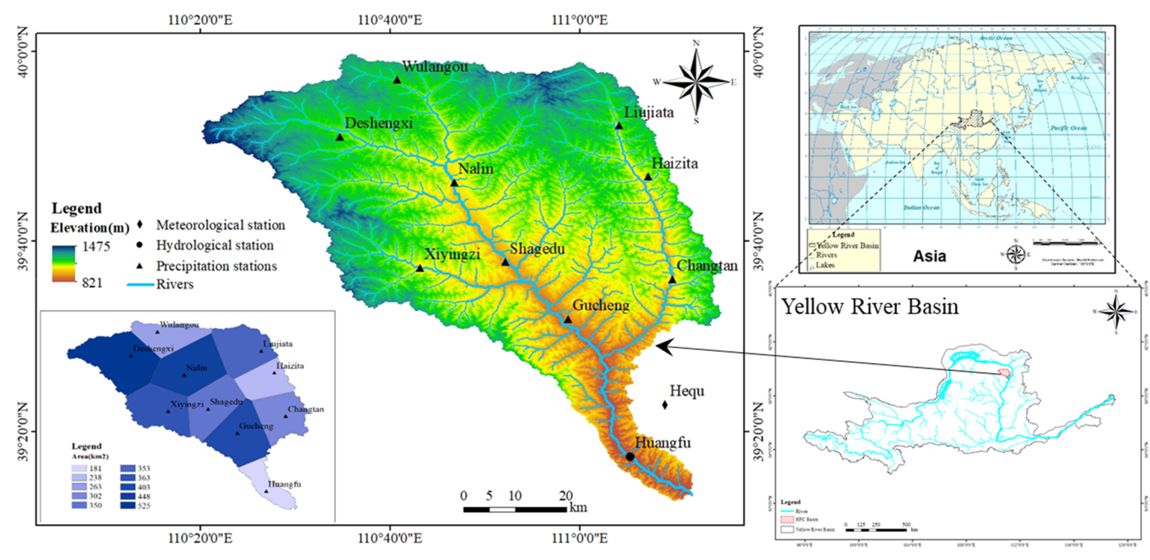
The Huangfuchuan Basin has an arid to semi-arid climate. The annual precipitation is low, and it mainly occurs as rainstorms. The water resources of the basin are relatively scarce, and their spatial and temporal distribution is uneven [39]. The ecological environment and socio-economic development in the basin are very sensitive to climate change, especially precipitation changes [40,41]. The basin is currently not affected by resource development, and the hydrological processes are mainly controlled by natural factors [42].
The Huangfuchuan Basin is located in the middle reaches of the Yellow River at 39.20°–39.90° N and 110.30°–111.15° E and is one of the major tributaries of the Yellow River, with an area of 3426 km2 and the length of mainstream is 137 km (Figure 1) [43]. The elevation ranged from 821 m to 1475 m. The annual precipitation of Huangfuchaun basin is between 350 mm and 450 mm, mainly concentrated in June to September, accounting for 80% of the annual precipitation [44], and often occurs over a relatively small area, and of short duration and high intensity [45]. The average annual temperature is 6.2–7.2 ℃, the annual sunshine hours are more than 3000 h, the annual relative humidity is 53%–56%.
2.2. Datasets
2.2.1. Observed Data
In this study, daily precipitation data for 10 stations from 1976 to 2012 in the Huangfuchuan Basin were obtained from the Yellow River Conservancy Commission (Table 1) [43]. The basin precipitation was calculated by the Thiessen Polygon method. The digital elevation model (DEM) with the horizontal resolution of 30 m in the Huangfuchuan Basin was obtained from International Scientific & Technical Data Mirror Site, Computer Network Information Center, Chinese Academy of Sciences (http://www.gscloud.cn/). The DEM was used to generate the river network and basin boundaries.
2.2.2. GCM Outputs
The GCM outputs were obtained from the Coupled Model Inter-comparison Project 5 (CMIP5) project of the IPCC Fifth Assessment Report (https://esgf-node.llnl.gov/search/cmip5). In this study, we selected 15 Global Climate Models under historical, Rcp2.6, Rcp4.5 and Rcp8.5 emission scenarios based on the relevant literature [46,47] to test the proposed downscaling method and forecast the future precipitation. Some scholars evaluated the applicability of these models in China [48,49]. The multi-model ensemble mean is, overall, superior to any individual model in reproducing the observed climate changes [50]. Therefore, the projections of precipitation under the representative concentration path (RCP) scenarios are derived from the arithmetic ensemble mean of the 15 GCMs’ outputs [51]. The information on the 15 global climate models is shown in Table 2. It is necessary to explain that, although IPCC provided the GCM daily precipitation data, we still needed GCM monthly precipitation data to drive the hydrological model. Maurer compared the utility of daily vs. monthly large-scale climate data, indicating that monthly GCM outputs are more credible and readily available than those on a daily scale [52]. Meanwhile, due to the coarse spatial resolution, if we chose GCM daily precipitation, it would have been more difficult to get accurate wet spells. For example, the inverse distance weighting (IDW) method was used to interpolate the GCM data at the four nearest neighboring grid points to the target site [53]. If the target site was located in a grid without rainfall, but the other grid had rainfall, wet spells would be increased artificially after interpolation. To be consistent with the observed data, the historical GCM monthly precipitation (1976–2005) was downloaded to test the performance of the proposed downscaling method. For climate change projections, the Rcp2.6, Rcp4.5 and Rcp8.5 scenarios were selected for 2021–2070 because our follow-up research will focus on the changes in water and sediment yield over the next 50 years based on the downscaling data.
2.3. Spatial Interpolation Method
The GCM outputs are stored as raster data, and the data are associated with the value of the entire grid cell. However, because the grid center is located at a distance from the precipitation station and a grid cell may include several precipitation stations, this is obviously unreasonable. Therefore, the GCM raster data need to be interpolated to the corresponding precipitation station using the spatial scale conversion method. Some studies have verified the feasibility of the inverse distance weighting (IDW) interpolation method in rainfall interpolation. Borges et al. compared the spatial interpolation method for an estimation of precipitation distribution, and the results showed the five interpolation methods, IDW included, that had the smallest error and the largest correlation coefficient and Nash coefficient [54]. Chen et al. used the inverse distance weighting method to estimate the spatial rainfall distribution in central Taiwan and proved the feasibility of the method [55]. Compared to the Kriging method, Cao proves that IDW method has better practicability, because the Kriging method requires more complex computation and takes more computation time, but the interpolation results are not significantly affected [56]. Therefore, IDW was chosen as the spatial interpolation method for precipitation in this study.
First, according to the latitude and longitude of precipitation stations, the nearest four grid center points were determined to calculate their angular distance from precipitation station [51]:
where D is the angular distance, θd is the latitude of the target precipitation station, ωd is the longitude of the target precipitation station, θs is the grid center latitude and ωs is the grid center longitude.
Second, we calculated the weight of each grid point [51]:
where Wi is the ith grid weight, n is the grid number.
Finally, the data of four grid center points were multiplied by their respective weight coefficients and added together to obtain the GCM data for the desired station.
2.4. Temporal Downscaling Method
2.4.1. Equidistant Cumulative Distribution Functions Matching Method (EDCDFm)
The principle of the Equidistant Cumulative Distribution Functions Matching Method (EDCDFm) is to modify the shape of the theoretical probability distribution function of the simulated precipitation data based on the shape of the theoretical probability distribution function of the observed precipitation data [57], and its deviation correction formula is as follows [58]:
where is the post-corrected GCM monthly data for a future period; xm-f is the pre-corrected GCM monthly data for a future period, () is the inverse function of the CDF of the observed (GCM output) monthly data for a current period and Fm-f is the CDF of the GCM monthly data for a future period.
This study used the mean, standard deviation, mean errors, relative deviation and Root Mean Square Error (RMSE) to evaluate the performance of corrected GCM monthly data. The calculation method is as follows:
where Sn and On are the simulated monthly data, and the observed monthly data, respectively.
2.4.2. CLIGEN Model
The CLIGEN model requires the following five input parameters to generate daily precipitation sequences for each month of the year [24]; it is a wet day when the precipitation amount is more than or equal to 0.1 mm:
- Average daily precipitation on wet days (Pw);
- Standard deviation of wet day precipitation (Sd);
- Coefficient of skewness of wet day precipitation (Skew);
- The probability of a wet day following a wet day (P(W|W));
- The probability of a wet day following a dry day (P(W|D)).
Therefore, when using the CLIGEN model to downscale GCM-generated monthly precipitation to daily precipitation sequences, these five parameters are needed for each month. The following procedure was followed to determine these parameter values:
(1) Observed daily precipitation data for 1976–2005 were first used to compute the mean (P_mon) and the variance (Var_mon), and the five CLIGEN parameters using daily observations, each month and for each site;
(2) A linear relationship between P_mon and P(W|D) for each month for all sites was assumed so that the wet-following-dry transition probability can be estimated for future years, i.e.,
(3) It was assumed that the probability of occurrence of a wet day, P(W), was proportional to P(W|D). In other words, since [59]:
it follows that:
(4) When changes in P(W|W) and P(W|D) are relatively small, it can be assumed that the variance in monthly precipitation is proportional to the variance in daily precipitation [59]. In this study, the changes of P(W|W) and P(W|D) from step (3) above are small (<0.02), so the standard deviation for climate projections based on the GCM data was calculated as follows:
where Sd and Sdo are the standard deviation of daily precipitation on wet days for GCM output and observed data, respectively, and Var and Varo are the variance of the monthly precipitation for GCM output and observed data, respectively.
The skewness coefficient of GCM output was assumed to be the same as the observed data.
2.4.3. Shuffle Procedure
Once the daily precipitation sequence was generated for each of the 10 sites in the Huangfuchuan Basin, the two-stage shuffle procedure was applied to re-create the spatial correlation of precipitation sequences for the ten stations, mainly following the method provided by Li [33] with two improvements:
(i) We used the Pearson correlation coefficient to adjust the input of the Spearman correlation coefficient.
The main steps are as follows:
1. A linear relationship was established and expressed as [Cos] = a × [Ccp] + b, where [Cos] was the observed Spearman correlation coefficient of the observed data, and [Ccp] was the Pearson correlation coefficient of the CLIGEN-generated data after shuffling (post-shuffled);
2. The input correlation coefficient was adjusted with the equation [Cos]’ = a × [Cop] + b, where [Cos]’ was the adjusted Spearman correlation coefficient of the observed data, and [Cop] was the desired (observed) Pearson correlation coefficient;
3. The new Spearman correlation coefficient ([Cos]’) was used to reshuffle the CLIGEN-generated precipitation sequences.
(ii) For the second shuffle phase, we rearranged the corresponding rows according to the precipitation occurrence structure of the wet days in the control station, and carried out random permutations for the dry days of each column. When we adjusted the rows of the post-shuffled precipitation matrix according to the control station, the corresponding rows in other columns were also rearranged simultaneously. Therefore, the Spearman rank and Pearson correlation coefficients were conserved.
3. Results
3.1. GCM Outputs Correction
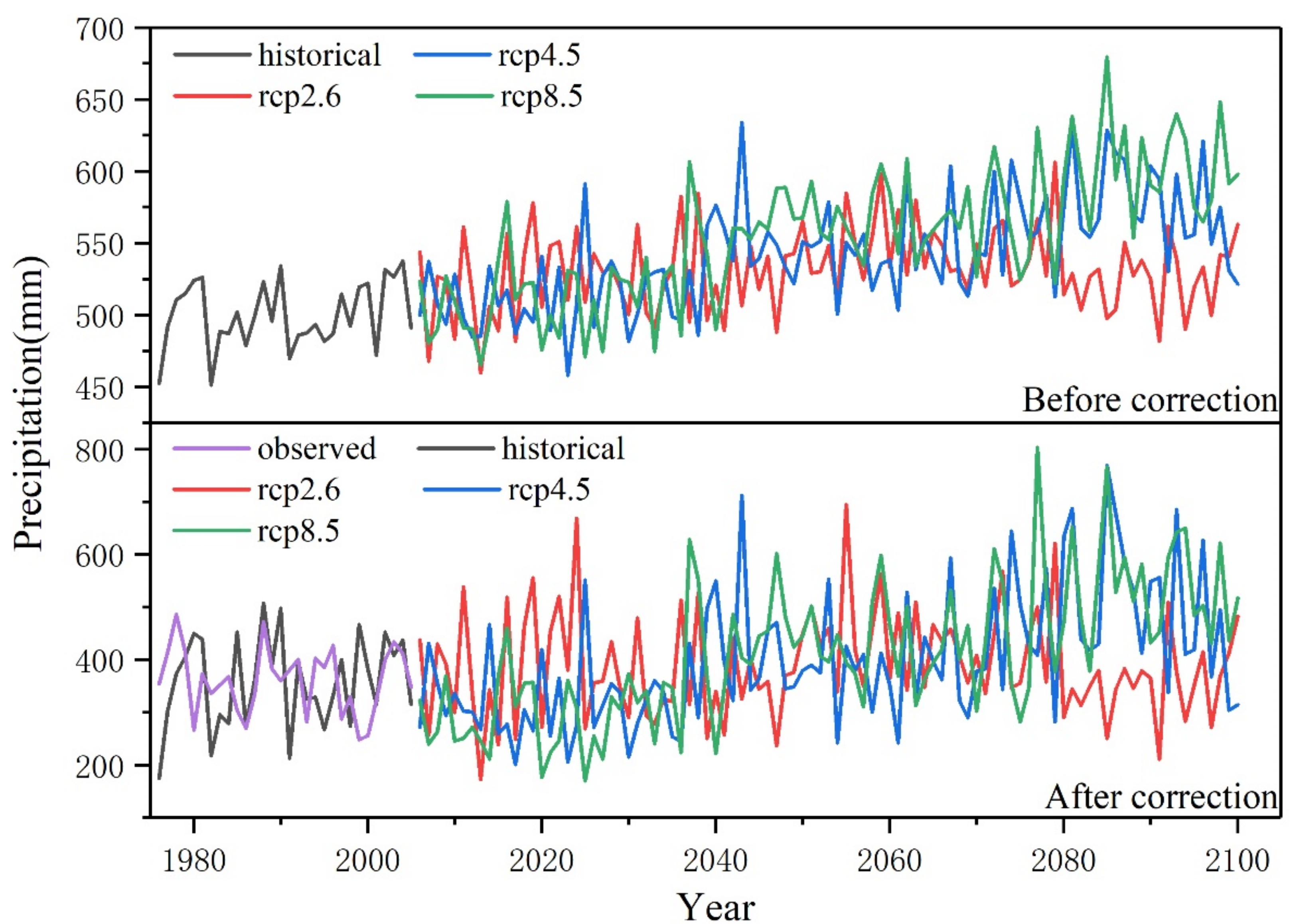
The monthly precipitation of the multi-model ensemble was corrected. This study used the Thiessen polygon method to calculate annual precipitation of the observed data, the pre-corrected GCM historical data and post-corrected GCM historical data in the Huangfuchuan Basin, respectively. The corresponding evaluation indicators are listed in Table 3. After correction, the average precipitation decreased from 499.70 mm to 357.64 mm, and the standard deviation changed from 22.83 mm to 85.02 mm. The results show that the evaluation indicators of post-corrected GCM historical data have been significantly improved, indicating that the EDCDF method is feasible. Therefore, we corrected the GCM projected data (Rcp2.6, Rcp4.5 and Rcp8.5 scenarios) for the next 50 years (2021–2070). The annual average precipitation under Rcp2.6, Rcp4.5 and Rcp8.5 scenarios from 2006 to 2100 is 389.30 mm, 400.72 mm, and 414.14 mm, respectively, indicating that the precipitation in this basin would show an increasing trend in the future, and the increase percentages were 8.50%, 11.69% and 15.43%, respectively, compared with the observed value (1976–2005).
A time series of the annual averaged precipitation in Huangfuchuan Basin from 1976 to 2100 for the multi-model ensemble is shown in Figure 2. Many studies show that China’s precipitation will increase in the future [48,50,51,60], and this trend also exists in this basin, but the inter-annual variation in GCM outputs before correction is smoother. This is because, compared to individual models, the model ensemble mean is, to a certain extent, able to reduce the spread among the models to better approach the observed changes and trends. However, it will also smooth the natural variability in the internal climate system [50]. After correction, the GCM output can increase the inter-annual variation and maintain the original data trend. Compared with the GCM outputs before correction, the standard deviation increased by 69.88 mm, 87.4 mm and 85.32 mm, respectively.
3.2. Evaluation of CLIGEN-generated Daily Precipitation Based on GCM Outputs without Using Shuffle Procedure
3.2.1. Applicability Evaluation of the Proposed Downscaling Method
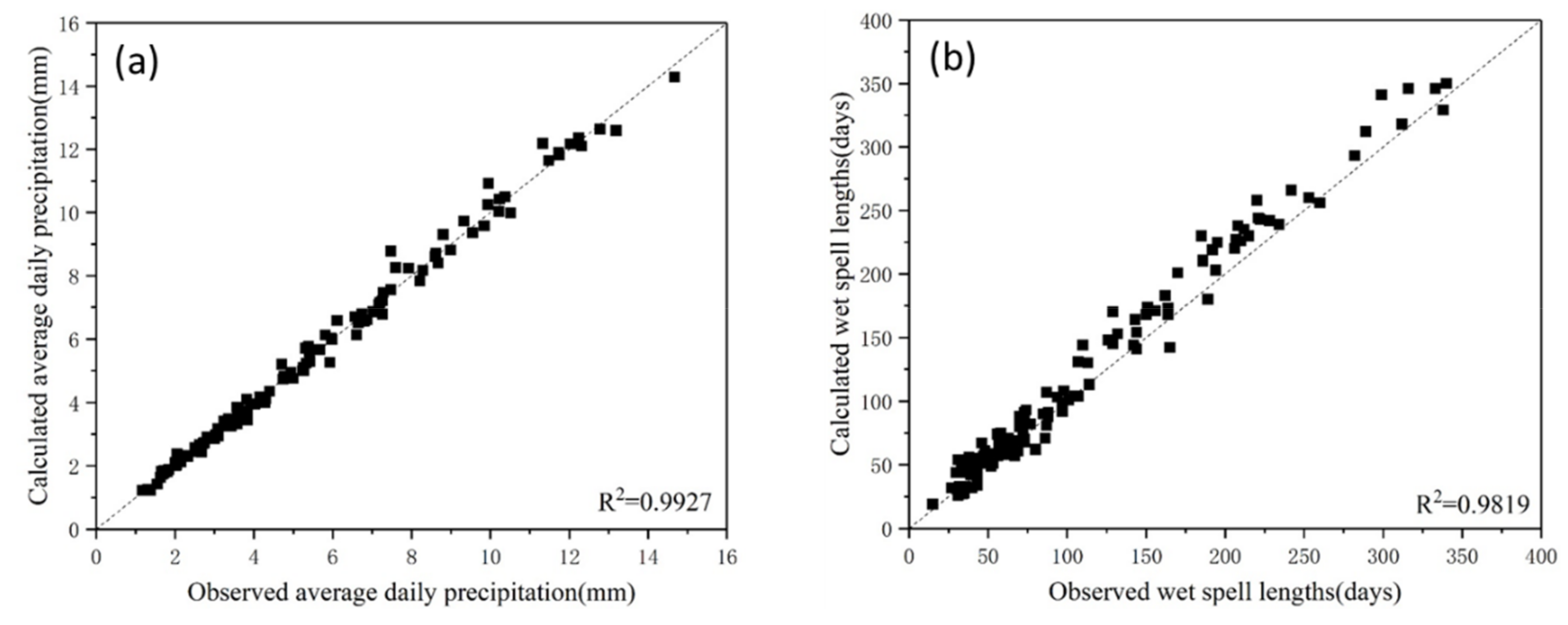
The daily precipitation sequences were generated based on observed statistical characteristics by the CLIGEN model, because the precipitation amount is controlled by precipitation on wet days and the number of wet days [61]. Thus, we calculated the average daily precipitation on wet days and the number of wet days in the generated precipitation sequences (Figure 3). The results showed that the calculated result had a good linear relationship with observed values and the R-square values were very close to one. The Nash coefficients were 0.99 and 0.96, respectively. Therefore, the proposed downscaling method can accurately simulate the change in the precipitation amount.
3.2.2. Evaluation of the Parameter α Value and R-square Value of Linear Equation
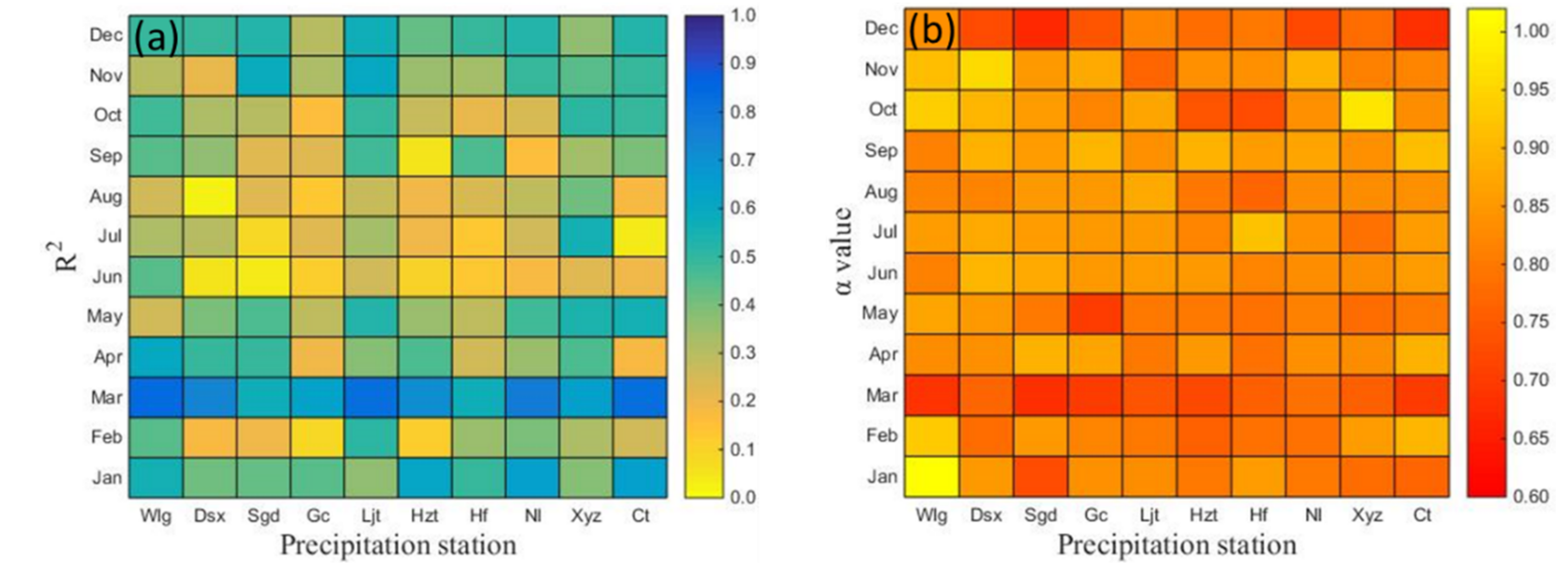
The linear relationship between observed average monthly precipitation and P(W|D) was established. Figure 4a shows that most of the R2 values were inversely proportional to their average monthly precipitation. Because P(W|D) reflected the probability of independent precipitation, it would decrease with precipitation increase. The magnitude and distribution characteristics of the coefficient α are shown in Figure 4b. The results show that the α values were mostly 0.6~1.0. However, the α value of Wulangou precipitation station in January was more than one. The question could be well understood, as when there was no continuous precipitation and precipitation did not occur on the first day of the month, the number of wet days following a dry day (Ndw) of the month should be equal to the wet days (Nw). The sum of Ndw and the number of wet days following a dry day (Ndd) was less than the total days of the month, so the P(W|D) (it can be calculated as follows: P(W|D) = Ndw/(Ndw + Ndd)) was more than the P(W) (which can be calculated as follows: P(W) = Nw / Nd). We assumed that the linear relationship and the α value remained unchanged for each month, and it was also possible to apply them to future studies, so the CLIGEN parameters of GCM precipitation data could be calculated.
3.2.3. Evaluation of Daily Precipitation Amount
The QQ plots were plotted in Figure 5 for ten precipitation stations. Figure 5 showed that when the precipitation was small, the downscaled GCM historical data had a good correspondence relationship with the observed data. As the precipitation increased, the deviation would occur, which also illustrated that the GLIGEN model had weaker ability to simulate the extreme value. Except for the Xiyingzi rainfall gauging station, the scatter points of other gauging stations were near the 1:1 line and we considered that the two distributions were similar in the historical period. The precipitation under the Rcp2.6 scenario is slightly more than the observed values, indicating that the daily precipitation will increase in the future. The precipitation under Rcp4.5 and Rcp8.5 scenarios shows that the precipitation in the low quantile will decrease and the precipitation in the high quantile will increase. Such precipitation distribution may increase the risk of future floods.
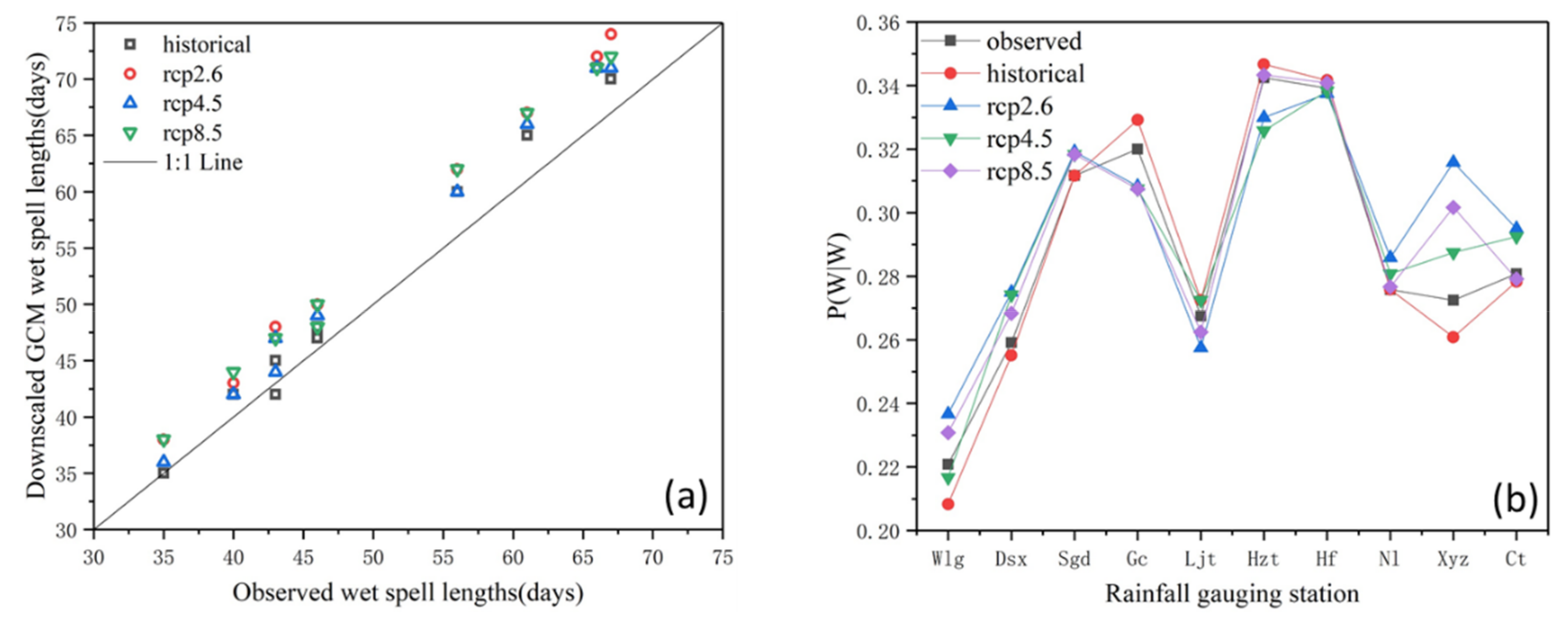
3.2.4. Evaluation of Aunual Average Wet Spell Lengths Lengths and P(W|W)
The downscaled GCM average wet spell lengths and P(W|W) were compared with the observations (Figure 6). Figure 6a illustrates that the pre-shuffled average historical wet spell lengths are slightly longer than the observed values for most rainfall gauging stations, but they had a good linear relationship, the Nash coefficient was 0.93, indicating that the downscaled GCM historical data can reproduce wet spell lengths very well. All of the wet spell lengths under Rcp2.6, Rcp4.5 and Rcp8.5 scenarios were larger than the observed values, indicating that the wet spell lengths will be an increasing trend in the future. Figure 6b illustrates the change in average P(W|W) (the probability of a wet day following a wet day) at ten rainfall gauging stations. The downscaled GCM historical P(W|W) has a good linear relationship with the observed values. Under the Rcp2.6, Rcp4.5 and Rcp8.5 scenario, the P(W|W) will increase at Deshengxi, Shagedu, Nalin and Xiyingzi rainfall gauging stations, while the P(W|W) will decrease at Gucheng and Haizita rainfall gauging stations. It also shows that the risk of flood may increase in some areas.
3.3. Reconstruction of Inter-Station Spatial Correlation of CLIGEN-Generated Daily Precipitation Sequences
In order to rebuild the inter-station spatial correlation, we should make the Pearson correlation coefficient of post-shuffled precipitation sequences equal to or closer to the observed Pearson correlation coefficient. However, it is very difficult to directly reconstruct the Pearson correlation coefficient. Some studies have shown that when there was a good linear relationship between the simulated Spearman correlation coefficient and the observations, the Pearson correlation coefficient of simulated data was closer to the observed values [62]. As a post-processing method, the shuffle procedure had been proven to effectively reconstruct the Spearman rank correlation [33,63]. Therefore, we rebuilt the Spearman rank correlation using Li’s method.
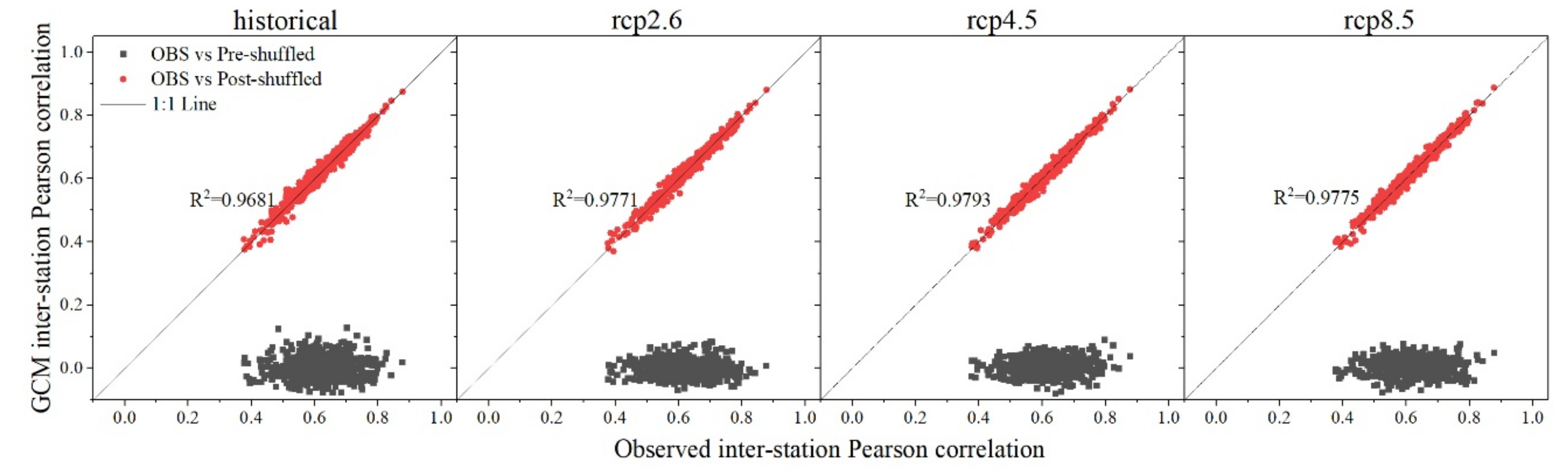
The inter-station spatial correlation was reconstructed based on the observed Spearman rank correlation coefficient. Figure 7 showed that the Spearman correlation coefficients of pre-shuffled historical data were between −0.1 and 0.2, and the linear correlation between the two groups of variables was weak. After using the shuffled procedure, the inter-station Spearman correlation coefficients were significantly improved and the R-squared values were very close to one, indicating that the shuffle procedure was effective in reconstructing the Spearman correlation coefficient.
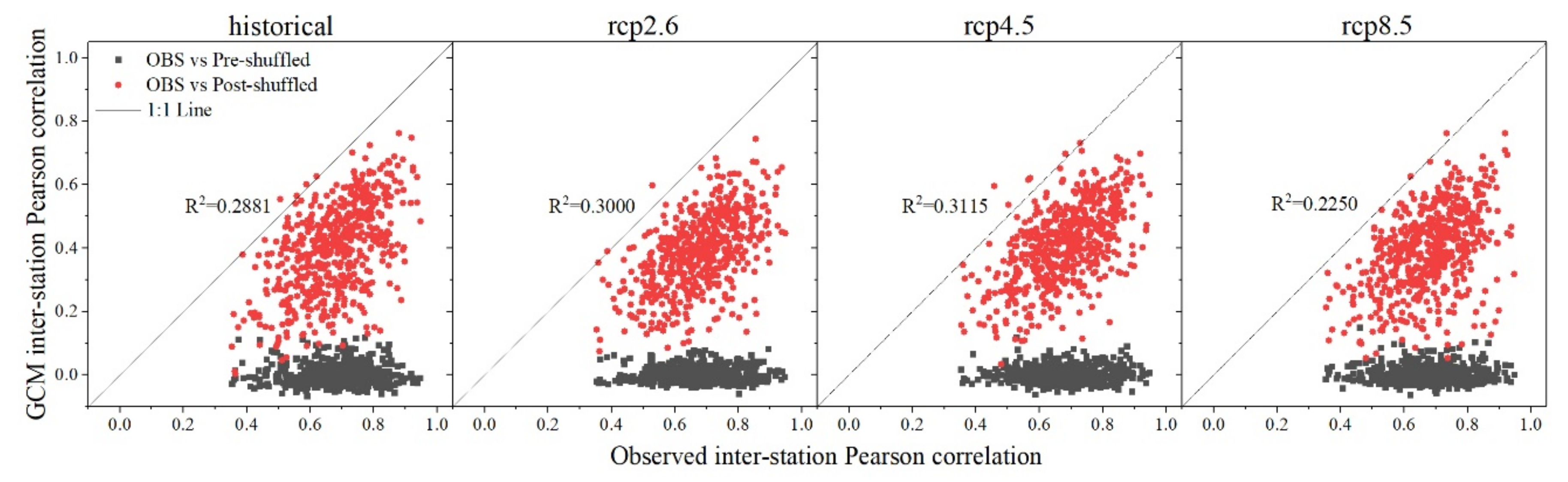
Meanwhile, we calculated the corresponding Pearson correlation coefficient of post-shuffled data using Li’s method (Figure 8). Although the inter-station spatial correlation was improved, the post-shuffled values were lower than the observations and R-square values were far less than one. In this study, the desired Pearson correlation coefficients were not obtained only using the observed Spearman rank correlation coefficient. This result also indicates that the aim of obtaining the desired Spearman rank correlation seems to be unimportant in rebuilding the spatial correlation. However, we could establish a linear relationship between the input Spearman correlation coefficients and the output Pearson correlation coefficients.
We tried to use the desired Pearson correlation coefficients to adjust the input Spearman correlation coefficients; meanwhile, the new shuffled results were obtained (Figure 9). The new post-shuffled results were closer to the observations compared to the old post-shuffled results. Figure 8 shows that the new scatter points can be better distributed on both sides of the 1:1 line, and the R-squared values are closer to one. Therefore, the modified shuffle procedure can be used to rebuild the spatial correlation of the CLIGEN-generated single-site precipitation sequences.
3.4. Evaluation of Post-Shuffled Daily Precipitation Sequences
The primary principle of the shuffle procedure is to rearrange the precipitation occurrence structure, while the precipitation amount and number of wet and dry days of post-shuffled data would not be changed. Therefore, we mainly evaluated some statistical characteristics related to the precipitation occurrence structure—for example, the probability of a wet day following a wet day (P(W|W)), the probability of a wet day following a dry day (P(W|D)) and annual precipitation. In order to conduct a more comprehensive evaluation, we added some statistical characteristics, including other CLIGEN parameters, except P(W|W), P(W|D) and average monthly precipitation. In fact, the added parameters were unaffected by the adjustment of the precipitation occurrence structure.
3.4.1. Comparison of CLIGEN Parameters between the Observed Data and the Downscaled GCM Data
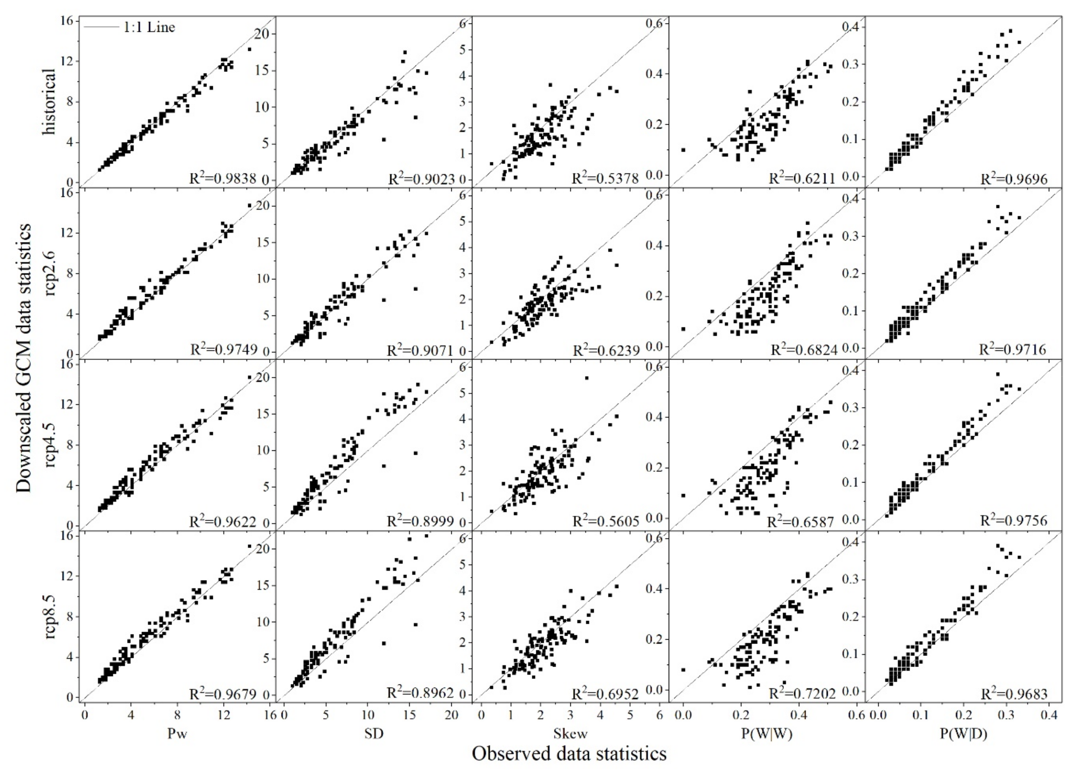
The five post-shuffled CLIGEN parameters were compared with the observed values (Figure 10). Figure 10 shows that in the historical scenario, the simulated results of average daily precipitation on wet days, standard deviation and P(W|D) of post-shuffled historical data are much better than other statistical characteristics, their R-square values are more than 0.9 and they have a better correspondence relationship with the observed values. The simulated results for the probability of a wet day following a wet day (P(W|W)) and the skewness coefficient of wet day precipitation (skew) of post-shuffled data are not good enough, but the R-square values are also more than 0.5. The simulated P(W|W) values are slightly smaller than the observed values; however, the simulated P(W|D) are slightly larger than the observed values. This is because P(W|W) and P(W|D) are calculated by the number of wet days following a wet day and the number of dry days following a wet day, and they show an inverse relationship. According to the previous analysis, the simulated historical wet spell length was larger than the observed values, and the precipitation was mainly on a single day. Thus, the simulated number of dry days following a wet day would be more, this result led to the simulated values being less than the observed values. The skewness coefficient was a statistical parameter reflecting the form of random series distribution. All of the simulated results were more than zero, indicating that the skew direction of distribution was consistent with the observed values; within the statistical characteristics of distribution exist errors.
The post-shuffled projected CLIGEN parameters were compared with the post-shuffled historical data. In terms of average daily precipitation on wet days (Pw), the projected values were more than the historical values. The increased values under Rcp2.6, Rcp4.5 and Rcp8.5 scenarios are 0.29, 0.38 and 0.48 mm, respectively. In the projection period, the simulated scatter points of standard deviation are more divergent, indicating that the differences in daily precipitation will increase in the future. The R-square values of the skewness coefficient are larger than the historical, indicating that the precipitation distribution in the future is more consistent with the observed values. Compared to the historical scenario, the P(W|W) shows significant differences, but the P(W|D) under Rcp2.6, Rcp4.5 and Rcp8.5 scenarios increases by 5.10%, 2.17% and 4.65%, respectively, indicating the wet spell lengths in the future will increase.
3.4.2. Comparison of Monthly and Annual Precipitation in the Huangfuchuan Basin
The catchment monthly precipitation of observed data, the post-shuffled historical data and the post-shuffled projected data were calculated and compared (Figure 11a). Figure 11a shows that the simulated historical monthly precipitation was generally consistent with the observed values; the simulated projected monthly precipitation was more than the observed values in most months. The average precipitation in summer and the percentage of summer precipitation as annual precipitation were calculated, respectively. The observed average summer precipitation was 235.03 mm, accounting for 65.51% of annual precipitation, and the simulated historical average precipitation in summer was 236.89 mm, accounting for 65.32% of annual precipitation. The simulated average summer precipitation is 1.86 mm more than the observation, and the Mean of Absolute value of Relative Error (hereafter denoted as MARE) was only 0.79%. The simulated average monthly precipitation was 0.32 mm more than the observed values, and the MARE was 1.08%. The above results indicated that the CLIGEN model was applicable to simulations of the monthly precipitation in the Huangfuchuan Basin and could be used to simulate monthly precipitation in the future. The simulated projected precipitation (Rcp2.6, Rcp4.5 and Rcp8.5 scenarios) was compared with the simulated historical data. The result shows an increasing trend, with percentage increases of 19.37%, 21.04% and 26.16%, respectively. In summer, due to the fact that the precipitation will increase, some measures for flood control and water and soil conservation are needed.
In terms of annual precipitation, nine kinds of datasets were compared (Figure 11b). The observed annual precipitation was 358.79 mm. The downscaled GCM historical annual precipitation was 362.65 mm and the corresponding MARE was 1.08%. The downscaled GCM average annual precipitation amounts under the Rcp2.6, Rcp4.5 and Rcp8.5 scenarios are 402.63, 393.06 and 405.01 mm, respectively. The observed maximum catchment annual precipitation was 485.70 mm, the downscaled historical calculation (pre-shuffle) was 413.42 mm and the corresponding MARE was 14.88%, the downscaled historical calculation (post-shuffle) was 541.40 mm and the corresponding MARE was 11.47%. The observed minimum catchment annual precipitation was 248.07 mm, the downscaled historical calculation (pre-shuffle) was 297.68 mm and the corresponding MARE was 20%, the downscaled historical calculation (post-shuffle) was 264.84 mm and the corresponding MARE was 5.06%. The above results indicated that the spatially uncorrelated precipitation sequences would affect the catchment extreme precipitation, and the shuffle procedure was effective for rebuilding the catchment extreme precipitation.
The extreme precipitation is often an important factor for water production and sediment yield, and accurate simulation results are required. This study’s introduced downscaling method can effectively solve this problem by rebuilding spatial correlation. Under Rcp2.6, Rcp4.5 and Rcp8.5 scenarios, the downscaled GCM maximum catchment annual precipitation amounts before using the shuffle procedure are 496.16, 467.08 and 517.33 mm, respectively; the downscaled GCM maximum catchment annual precipitation amounts after using the shuffle procedure are 655.11, 683.94 and 709.89 mm, respectively. After using the shuffle procedure, the range of annual precipitation can effectively increase. The above results show that both the maximum and average annual precipitation is largest in the Rcp8.5 scenario, indicating the annual precipitation change is the most significant in this scenario.
3.5. Comparison of Spatial Distribution of Annual Precipitation
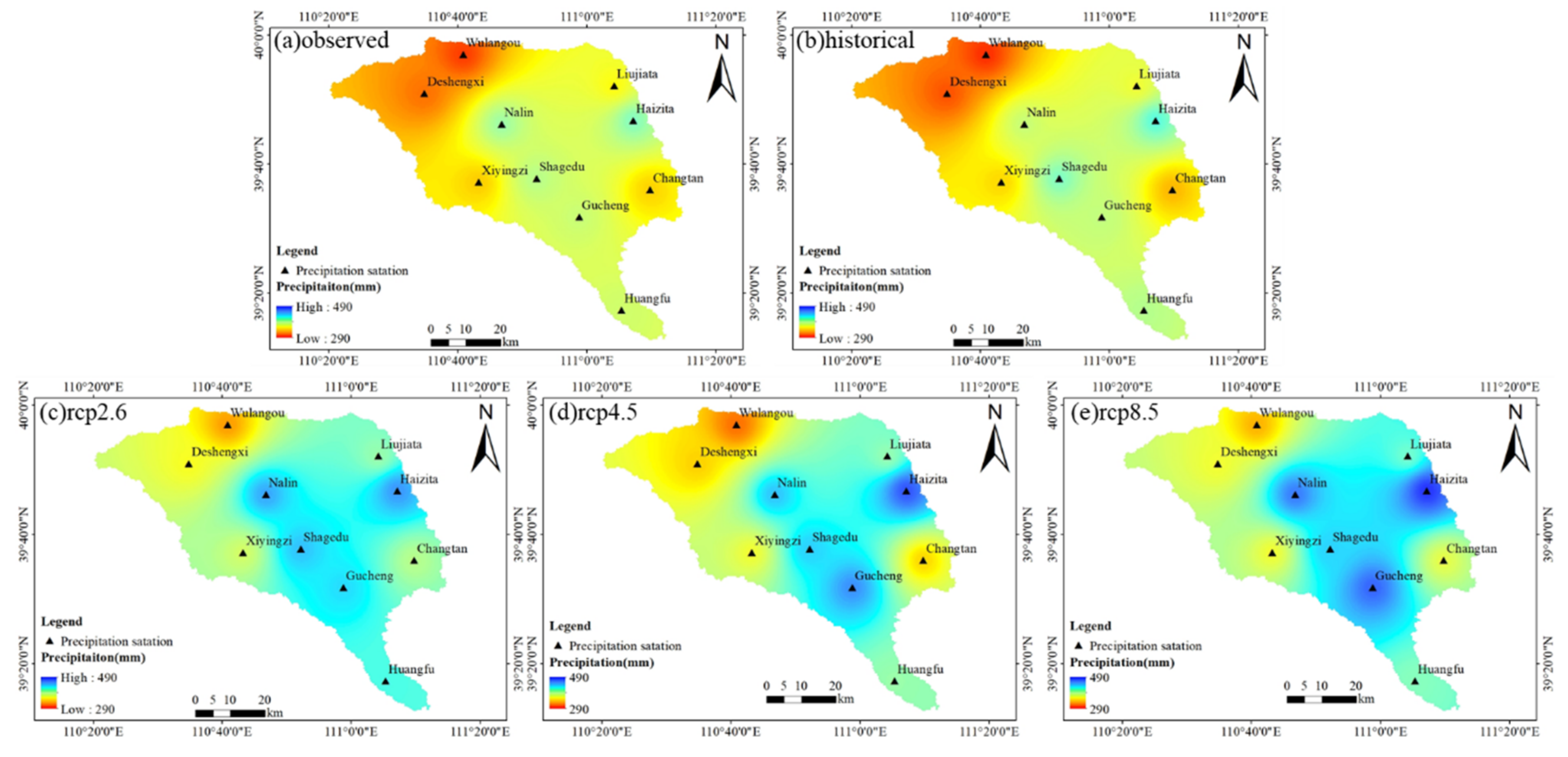
According to the observed annual precipitation and the downscaled GCM annual precipitation for ten rainfall gauging station, we used the inverse distance weighting method to get the spatial distribution map of average annual precipitation, which is shown in Figure 12. It shows that the there is no significant change in the location of the rain center, which is mainly concentrated in the middle of the basin. The northwest of the basin has the least precipation. The spatial distribution of the downscaled historical precipitation is almost consistent with the observed result, indicating the proposed method can simulate spatial ditribution very well. Under Rcp2.6, Rcp4.5 and Rcp8.5 scenarios, the amount of precipitation has an obvious increase trend. In order to better cope with climate change, the main control measures should be concentrated in the middle of the basin in the future management processes.
4. Discussion
CLIGEN is a stochastic weather generator established by the United States Department of Agriculture (USDA) to provide a climate input for Water Erosion Prediction Project (WEPP) model [14,15], which includes daily precipitation, precipitation pattern, maximum and minimum temperature, dew temperature, wind direction, wind speed and solar radiation [16], its feasibility has been verified by many scholars [9,14,17,18,24,25,27,61]. However, due to the fact that it is a single-site weather generator and there is no mature method to calculate the parameters based on the GCM outputs, its application is limited. This study used the modified shuffle procedure proposed by Li [33] to address the problem of the spatially uncorrelated downscaled CLIGEN-generated data. Meanwhile, we proposed a method to calculate the CLIGEN precipitation parameters based on GCM monthly outputs. The application range of the CLIGEN model is greatly improved. The proposed downscaling method can provide a powerful support to study region climate change and hydrological processes.
Firstly, in order to reduce the uncertainty of GCM outputs, we used the CMIP5 multi-model ensemble to study climate change in the future. Some studies show that, compared to individual models, the model ensemble mean is, to a certain extent, able to reduce the spread among the models to better approach the observed changes and trends [51,60]. The result shows that the future annual precipitation will increase in the Huangfuchuan Basin, the increment from large to small is Rcp8.5, Rcp4.5 and Rcp2.6, respectively. However, we also note that it smooths out the natural variability of the internal climate system. Therefore, it should be used with caution to study extreme climate change [50].
Secondly, the shuffle procedure was used to reconstruct the spatial correlation of the CLIGEN-generated independently precipitation sequences, and thus the spatial correlation was significantly improved after shuffling. However, there are only 10 precipitation stations in study area. As the study area increases, the number of precipitation stations also increases. Correspondingly, the inter-station spatial correlation decreases. Future studies will further explore the feasibility of the proposed method in large-scale river basins.
Finally, we found that the proposed downscaling method has some errors in the simulation of P(W|W) and skewness coefficient. This is because in the CLIGEN model, the precipitation occurrence structure mainly depends on the first-order two-state Markov chain. Although this Markov chain has already been proven to have good applicability in simulating the probability of precipitation transition [64], errors will still occur, because the Markov chain lacks physical mechanisms. Many scholars have tried to simulate the precipitation transition probability by using a high-order multi-state Markov chain [65,66], and obtained good results. Therefore, in order to simulate the occurrence of precipitation more accurately, it is necessary to properly modify the first-order two-state Markov chain.
We know that there are two kinds of downscaling method: dynamic downscaling method and statistical downscaling method. The physical mechanism of the dynamic downscaling method is clear, and it is not limited by the observation data. It can accurately simulate the characteristics of regional climate variables. Some studies show that he grid-based precipitation data generated through dynamical downscaling is able to better characterize the spatial pattern of precipitation and convection processes of a catchment scale [67,68]. However, the computational cost of dynamical downscaling is relatively high, and, due to the inherited GCM bias, as well as the bias caused by its own incomplete understanding of the climate system, the results cannot be directly used to assess the runoff response at the watershed scale or site scale [69]. The statistical downscaling method can make up the deficiency of the dynamic downscaling method to some extent [70]. Future research will try to combine the statistical downscaling method and dynamic downscaling method, and combine the advantages of their respective methods to provide better technical support for coping with climate change.
5. Conclusions
In order to better cope with the potential impact of climate change, people pay more attention to the understanding of future climate conditions. Moreover, the GCM outputs can meet people’s needs. However, due to its coarse temporal and spatial resolution, an effective downscaling method is often needed to provide a strong support for the study of regional climatic conditions and regional hydrological process simulations. This study proposed a multi-site downscaling method based on CLIGEN model and modified shuffle procedure. The CMIP5 multi-model ensemble monthly precipitation data for ten precipitation stations in the Huangfuchuan Basin were downscaled. The GCM data was divided into two parts: the historical period (1976–2005) and the future period (Rcp2.6, Rcp4.5 and Rcp8.5 scenarios, 2021–2070), which were used for testing and forecasting, respectively. The result show (i) the proposed downscaling method can be used to address the problem of the coarse temporal and spatial resolution of GCM data; (ii) the precipitation will increase in the projected period (2021–2070) and, in terms of average daily precipitation, monthly precipitation and maximum annual precipitation, the increment from large to small is Rcp8.5, Rcp4.5 and Rcp2.6, respectively. More precipitation will increase the risk of flooding and soil erosion in the basin, and some measures should be taken to prevent and control it. The main contributions of this study are (i) to verify the feasibility of the modified shuffle procedure for data spatial correlation reconstruction, as a post-processing technology, which provides a possible way to process not only data from other single point downscaling methods, but also other meteorological data, such as temperature and humidity and (ii) to describe the characteristics of future regional climate change based on a CMIP5 multi-model ensemble. Future research should focus on verifying the feasibility of this approach in different climate regions and combining it with hydrological models to help us understand changes in hydrological processes in the context of climate change.
Author Contributions
Conceptualization, X.S. and W.S.; methodology, X.S.; validation, X.S.; formal analysis, X.S., W.S., J.L. and Y.J.; investigation, X.S.; resources, J.L. and Y.J.; data curation, X.S.; writing—original draft preparation, X.S.; writing—review and editing, X.S., W.S., J.L. and Y.J.; visualization, X.S.; supervision, W.S.; funding acquisition, W.S., L.J. and Y.J. All authors have read and agreed to the published version of the manuscript.
Funding
This research was funded by Chinese National Key Research and Development Program, grant number 2018YFC1508203, Chinese National Natural Science Foundation, grant numbers 51739011, 51879274 and 51979285, Research Fund of the China Institute of Water Resources and Hydropower Research, grant numbers WR0145B502016 and 2017ZY02.
Acknowledgments
Thanks are given to the anonymous reviewers and editors for their constructive comments.
Conflicts of Interest
The authors declare no conflict of interest.
References
- Pachauri, R.K.; Allen, M.R.; Barros, V.R.; Broome, J.; Cramer, W.; Christ, R.; Church, J.A.; Clarke, L.; Dahe, Q.; Dasgupta, P.; et al. Climate Change 2014: Synthesis Report. Contribution of Working Groups I, II and III to the Fifth Assessment Report of the Intergovernmental Panel on Climate Change; Intergovernmental Panel on Climate Change: Geneva, Switzerland, 2014. [Google Scholar]
- Neupane, R.P.; White, J.D.; Alexander, S.E. Projected hydrologic changes in monsoon-dominated Himalaya Mountain basins with changing climate and deforestation. J. Hydrol. 2015, 525, 216–230. [Google Scholar] [CrossRef]
- Teklesadik, A.D.; Alemayehu, T.; Van Griensven, A.; Kumar, R.; Liersch, S.; Eisner, S.; Tecklenburg, J.; Ewunte, S.; Wang, X. Inter-model comparison of hydrological impacts of climate change on the Upper Blue Nile basin using ensemble of hydrological models and global climate models. Clim. Chang. 2017, 141, 517–532. [Google Scholar] [CrossRef]
- Shrestha, B.; Cochrane, T.A.; Caruso, B.S.; Arias, M.E.; Piman, T. Uncertainty in flow and sediment projections due to future climate scenarios for the 3S Rivers in the Mekong Basin. J. Hydrol. 2016, 540, 1088–1104. [Google Scholar] [CrossRef]
- Kim, Y.D.; Kim, J.M.; Kang, B. Projection of runoff and sediment yield under coordinated climate change and urbanization scenarios in Doam dam watershed, Korea. J. Water Clim. Chang. 2017, 8, 235–253. [Google Scholar] [CrossRef]
- Mondal, A.; Khare, D.; Kundu, S.; Meena, P.K.; Mishra, P.K.; Shukla, R. Impact of climate change on future soil erosion in different slope, land use, and soil-type conditions in a part of the Narmada River Basin, India. J. Hydrol. Eng. 2015, 20, C5014003. [Google Scholar] [CrossRef]
- de Hipt, F.O.; Diekkrüger, B.; Steup, G.; Yira, Y.; Hoffmann, T.; Rode, M. Modeling the impact of climate change on water resources and soil erosion in a tropical catchment in Burkina Faso, West Africa. Catena 2018, 163, 63–77. [Google Scholar] [CrossRef]
- Maraun, D.; Wetterhall, F.; Ireson, A.M.; Chandler, R.E.; Kendon, E.J.; Widmann, M.; Brienen, S.; Rust, H.W.; Sauter, T.; Themeßl, M.; et al. Precipitation downscaling under climate change: Recent developments to bridge the gap between dynamical models and the end user. Rev. Geophys. 2010, 48. [Google Scholar] [CrossRef]
- Nicks, A.D.; Gander, G.A. CLIGEN: A Weather Generator for Climate Inputs to Water Resource and Other Models. In Proceedings of the 5th International Conference on Computers in Agricultural, Orlando, FL, USA, 6–9 February 1994; pp. 903–909. [Google Scholar]
- Sharpley, A.N.; Williams, J.R. EPIC-Erosion/Productivity Impact Calculator. I: Model Documentation. II: User Manual; US Department of Agriculture: Washington, DC, USA, 1990.
- Richardson, C.W.; Wright, D.A. WGEN: A Model for Generating Daily Weather Variables; US Department of Agriculture, Agricultural Research Service: Washington, DC, USA, 1984; p. 83.
- Hanson, C.L.; Cumming, K.A.; Woolhiser, D.A.; Richardson, C.W. Microcomputer Program for Daily Weather Simulation in the Contiguous United States; ARS: Washington, DC, USA, 1994. [Google Scholar]
- Semenov, M.A.; Barrow, E.M. Use of a stochastic weather generator in the development of climate change scenarios. Clim. Chang. 1997, 35, 397–414. [Google Scholar] [CrossRef]
- Kinnell, P.I. CLIGEN as a weather generator for RUSLE2. Catena 2019, 172, 877–880. [Google Scholar] [CrossRef]
- Vu, T.M.; Mishra, A.K.; Konapala, G.; Liu, D. Evaluation of multiple stochastic rainfall generators in diverse climatic regions. Stoch. Environ. Res. Risk Assess. 2018, 32, 1337–1353. [Google Scholar] [CrossRef]
- Anache, J.A.; Flanagan, D.C.; Srivastava, A.; Wendland, E.C. Land use and climate change impacts on runoff and soil erosion at the hillslope scale in the Brazilian Cerrado. Sci. Total Environ. 2018, 622, 140–151. [Google Scholar] [CrossRef]
- Vaghefi, P.; Yu, B. Validation of CLIGEN Parameter Adjustment Methods for Southeastern Australia and Southwestern Western Australia. J. Hydrometeorol. 2017, 18, 2011–2028. [Google Scholar] [CrossRef]
- Chen, J.; Gitau, M.W.; Engel, B.A.; Flanagan, D.C. Suitability of CLIGEN precipitation estimates based on a n updated database and their impacts on urban runoff: A case study of the Great Lakes Region, USA. Hydrol. Sci. J. 2018, 63, 1502–1518. [Google Scholar] [CrossRef]
- Li, Z.; Shi, X.; Li, J. Multisite and multivariate GCM downscaling using a distribution-free shuffle procedure for correlation reconstruction. Clim. Res. 2017, 72, 141–151. [Google Scholar] [CrossRef]
- Hoomehr, S.; Schwartz, J.S.; Yoder, D.C. Potential changes in rainfall erosivity under GCM climate change scenarios for the southern Appalachian region, USA. Catena 2016, 136, 141–151. [Google Scholar] [CrossRef]
- Trotochaud, J.; Flanagan, D.C.; Engel, B.A. A simple technique for obtaining future climate data inputs for natural resource models. Appl. Eng. Agric. 2016, 32, 371–381. [Google Scholar] [CrossRef] [Green Version]
- Zhang, X.C. A comparison of explicit and implicit spatial downscaling of GCM output for soil erosion and crop production assessments. Clim. Chang. 2007, 84, 337–363. [Google Scholar] [CrossRef]
- Johnson, G.L.; Hanson, C.L.; Hardegree, S.P.; Ballard, E.B. Stochastic weather simulation: Overview and analysis of two commonly used models. J. Appl. Meteorol. 1996, 35, 1878–1896. [Google Scholar] [CrossRef] [Green Version]
- Vaghefi, P.; Yu, B. Use of CLIGEN to simulate decreasing precipitation trends in the southwest of Western Australia. Trans. ASABE 2016, 59, 49–61. [Google Scholar] [CrossRef]
- Elliot, W.J.; Arnold, C.D. Validation of the weather generator CLIGEN with precipitation data from Uganda. Trans. ASAE 2001, 44, 53. [Google Scholar] [CrossRef]
- Chen, Y.D.; Chen, X.; Xu, C.Y.; Shao, Q. Downscaling of daily precipitation with a stochastic weather generator for the subtropical region in South China. Hydrol. Earth Syst. Sci. Discuss. 2006, 3, 1145–1183. [Google Scholar] [CrossRef]
- Kou, X.; Ge, J.; Wang, Y.; Zhang, C. Validation of the weather generator CLIGEN with daily precipitation data from the Loess Plateau, China. J. Hydrol. 2007, 347, 347–357. [Google Scholar] [CrossRef]
- Li, X.; Zhang, K.; Babovic, V. Projections of Future Climate Change in Singapore Based on a Multi-Site Multivariate Downscaling Approach. Water 2019, 11, 2300. [Google Scholar] [CrossRef] [Green Version]
- Chen, J.; Chen, H.; Guo, S. Multi-site precipitation downscaling using a stochastic weather generator. Clim. Dyn. 2018, 50, 1975–1992. [Google Scholar] [CrossRef]
- Li, X.; Babovic, V. Multi-site multivariate downscaling of global climate model outputs: An integrated framework combining quantile mapping, stochastic weather generator and Empirical Copula approaches. Clim. Dyn. 2019, 52, 5775–5799. [Google Scholar] [CrossRef]
- Wilks, D.S. Multisite generalization of a daily stochastic precipitation generation model. J. Hydrol. 1998, 210, 178–191. [Google Scholar] [CrossRef]
- Brissette, F.P.; Khalili, M.; Leconte, R. Efficient stochastic generation of multi-site synthetic precipitation data. J. Hydrol. 2007, 345, 121–133. [Google Scholar] [CrossRef]
- Li, Z. A new framework for multi-site weather generator: A two-stage model combining a parametric method with a distribution-free shuffle procedure. Clim. Dyn. 2014, 43, 657–669. [Google Scholar] [CrossRef]
- Chen, J.; Brissette, F.P.; Zhang, X.J. A multi-site stochastic weather generator for daily precipitation and temperature. Trans. ASABE 2014, 57, 1375–1391. [Google Scholar] [CrossRef]
- Srivastav, R.K.; Simonovic, S.P. Multi-site, multivariate weather generator using maximum entropy bootstrap. Clim. Dyn. 2015, 44, 3431–3448. [Google Scholar] [CrossRef]
- Salehnia, N.; Hosseini, F.; Farid, A.; Kolsoumi, S.; Zarrin, A.; Hasheminia, M. Comparing the performance of dynamical and statistical downscaling on historical run precipitation data over a semi-arid region. Asia Pac. J. Atmos. Sci. 2019, 55, 737–749. [Google Scholar] [CrossRef]
- Sachindra, D.A.; Ahmed, K.; Rashid, M.M.; Shahid, S.; Perera, B.J. Statistical downscaling of precipitation using machine learning techniques. Atmos. Res. 2018, 212, 240–258. [Google Scholar] [CrossRef]
- Onyutha, C.; Tabari, H.; Rutkowska, A.; Nyeko-Ogiramoi, P.; Willems, P. Comparison of different statistical downscaling methods for climate change rainfall projections over the Lake Victoria basin considering CMIP3 and CMIP5. J. Hydro Environ. Res. 2016, 12, 31–45. [Google Scholar] [CrossRef]
- Shi, H.Y.; Li, T.J.; Zhu, J.F.; Zhang, A. Impact of Check Dams on the Sharp Decrease of Runoff in the Middle Yellow River: Case Study in the Huangfuchuan River Basin. In Proceedings of the International Yellow River Forum, Zhengzhou, China, 24–28 September 2012; pp. 461–462. [Google Scholar] [CrossRef]
- Yang, Q. Baseflow Change of Different Geomorphologic Regions in the Middle Yellow River and Its Responses to Ecological Construction; Xi’an University of Technology: Xi’an, China, 2019. [Google Scholar]
- Yang, Q.; Li, Z.; Han, Y.; Gao, H. Responses of Baseflow to Ecological Construction and Climate Change in Different Geomorphological Types in The Middle Yellow River, China. Water 2020, 12, 304. [Google Scholar] [CrossRef] [Green Version]
- Wang, W.L.; Li, Z.B.; Zhang, P.C.; Liu, M. Study on the development characteristics of debris flow in huangfuchuan river basin in the sandy and coarse sand area. Yellow River 2003, 25, 18–19. [Google Scholar]
- Li, E.; Mu, X.; Zhao, G.; Gao, P.; Sun, W. Effects of check dams on runoff and sediment load in a semi-arid river basin of the Yellow River. Stoch. Environ. Res. Risk Assess. 2017, 31, 1791–1803. [Google Scholar] [CrossRef]
- Chen, Y.; Guan, Y.; Shao, G.; Zhang, D. Investigting trends in streamflow and precipitation in Huangfuchuan Basin with wavelet analysis and the Mann-Kendall test. Water 2016, 8, 77. [Google Scholar] [CrossRef] [Green Version]
- Hu, Z.; Wang, L.; Wang, Z.; Hong, Y.; Zheng, H. Quantitative assessment of climate and human impacts on surface water resources in a typical semi-arid watershed in the middle reaches of the Yellow River from 1985 to 2006. Int. J. Climatol. 2015, 35, 97–113. [Google Scholar] [CrossRef]
- Chen, L.; Frauenfeld, O.W. A comprehensive evaluation of precipitation simulations over China based on CMIP5 multimodel ensemble projections. J. Geophys. Res. Atmos. 2014, 119, 5767–5786. [Google Scholar] [CrossRef]
- Wang, L.; Chen, W. A CMIP5 multimodel projection of future temperature, precipitation, and climatological drought in China. Int. J. Climatol. 2014, 34, 2059–2078. [Google Scholar] [CrossRef]
- Ying, X.; Chong-Hai, X.U. Preliminary assessment of simulations of climate changes over China by CMIP5 multi-models. Atmos. Ocean. Sci. Lett. 2012, 5, 489–494. [Google Scholar] [CrossRef]
- Jia, W.U.; Bo-Tao, Z.; Ying, X.U. Response of precipitation and its extremes over China to warming: CMIP5 simulation and projection. Chin. J. Geophys. 2015, 58, 461–473. [Google Scholar] [CrossRef]
- Zhao, T.; Chen, L.; Ma, Z. Simulation of historical and projected climate change in arid and semiarid areas by CMIP5 models. Chin. Sci. Bull. 2014, 59, 412–429. [Google Scholar] [CrossRef]
- Chong-Hai, X.U.; Ying, X. The projection of temperature and precipitation over China under RCP scenarios using a CMIP5 multi-model ensemble. Atmos. Ocean. Sci. Lett. 2012, 5, 527–533. [Google Scholar] [CrossRef] [Green Version]
- Maurer, E.P.; Hidalgo, H.G. Utility of daily vs. monthly large-scale climate data: An intercomparison of two statistical downscaling methods. Hydrol. Earth Syst. Sci. 2008, 12, 551–563. [Google Scholar] [CrossRef] [Green Version]
- Li, Z.; Liu, W.Z.; Zhang, X.C.; Zheng, F.L. Assessing the site-specific impacts of climate change on hydrology, soil erosion and crop yields in the Loess Plateau of China. Clim. Chang. 2011, 105, 223–242. [Google Scholar] [CrossRef]
- de Amorim Borges, P.; Franke, J.; da Anunciação, Y.M.; Weiss, H.; Bernhofer, C. Comparison of spatial interpolation methods for the estimation of precipitation distribution in Distrito Federal, Brazil. Theor. Appl. Climatol. 2016, 123, 335–348. [Google Scholar] [CrossRef]
- Chen, F.W.; Liu, C.W. Estimation of the spatial rainfall distribution using inverse distance weighting (IDW) in the middle of Taiwan. Paddy Water Environ. 2012, 10, 209–222. [Google Scholar] [CrossRef]
- Cao, Y. Comparison of Three Methods for the Spatial Interpolation of Rainfall Data; Technical University of Munich: Munich, Germany, 2017. [Google Scholar]
- Chen, J.; Brissette, F.P.; Chaumont, D.; Braun, M. Performance and uncertainty evaluation of empirical downscaling methods in quantifying the climate change impacts on hydrology over two North American river basins. J. Hydrol. 2013, 479, 200–214. [Google Scholar] [CrossRef]
- Li, H.; Sheffield, J.; Wood, E.F. Bias correction of monthly precipitation and temperature fields from Intergovernmental Panel on Climate Change AR4 models using equidistant quantile matching. J. Geophys. Res. Atmos. 2010, 115. [Google Scholar] [CrossRef]
- Zhang, X.C.; Nearing, M.A.; Garbrecht, J.D.; Steiner, J.L. Downscaling monthly forecasts to simulate impacts of climate change on soil erosion and wheat production. Soil Sci. Soc. Am. J. 2004, 68, 1376–1385. [Google Scholar] [CrossRef] [Green Version]
- Wang, X.; Yang, T.; Li, X.; Shi, P.; Zhou, X. Spatio-temporal changes of precipitation and temperature over the Pearl River basin based on CMIP5 multi-model ensemble. Stoch. Environ. Res. Risk Assess. 2017, 31, 1077–1089. [Google Scholar] [CrossRef]
- Yu, B. Adjustment of CLIGEN parameters to generate precipitation change scenarios in southeastern Australia. Catena 2005, 61, 196–209. [Google Scholar] [CrossRef]
- Tarpanelli, A.; Franchini, M.; Brocca, L.; Camici, S.; Melone, F.; Moramarco, T. A simple approach for stochastic generation of spatial rainfall patterns. J. Hydrol. 2012, 472, 63–76. [Google Scholar] [CrossRef]
- Iman, R.L.; Conover, W.J. A distribution-free approach to inducing rank correlation among input variables. Commun. Stat. Simul. Comput. 1982, 11, 311–334. [Google Scholar] [CrossRef]
- Gregory, J.M.; Wigley, T.M.L.; Jones, P.D. Determining and interpreting the order of a two-state Markov Chain: Application to models of daily precipitation. Water Resour. Res 1992, 28, 1443–1446. [Google Scholar] [CrossRef]
- Mehrotra, R.; Srikanthan, R.; Sharma, A. A comparison of three stochastic multi-site precipitation occurrence generators. J. Hydrol. 2006, 331, 280–292. [Google Scholar] [CrossRef]
- Lennartsson, J.; Baxevani, A.; Chen, D. Modelling precipitation in Sweden using multiple step Markov chains and a composite model. J. Hydrol. 2008, 363, 42–59. [Google Scholar] [CrossRef] [Green Version]
- Wang, S.; Wang, Y. Improving probabilistic hydroclimatic projections through high-resolution convection-permitting climate modeling and Markov chain Monte Carlo simulations. Clim. Dyn. 2019, 53, 1613–1636. [Google Scholar] [CrossRef]
- Zhang, B.; Wang, S.; Wang, Y. Copula-Based Convection-Permitting Projections of Future Changes in Multivariate Drought Characteristics. J. Geophys. Res. Atmos. 2019, 124, 7460–7483. [Google Scholar] [CrossRef]
- Teutschbein, C.; Seibert, J. Bias correction of regional climate model simulations for hydrological climate-change impact studies: Review and evaluation of different methods. J. Hydrol. 2012, 456, 12–29. [Google Scholar] [CrossRef]
- Murphy, J. An evaluation of statistical and dynamical techniques for downscaling local climate. J. Clim. 1999, 12, 2256–2284. [Google Scholar] [CrossRef]
Figure 1.
Location of study area and distribution of precipitation stations, hydrological station and meteorological station (elevation derived from the 30 m digital elevation model (DEM)).
Figure 1.
Location of study area and distribution of precipitation stations, hydrological station and meteorological station (elevation derived from the 30 m digital elevation model (DEM)).

Figure 2.
Time series of annual averaged precipitation in Huangfuchuan Basin from 1976 to 2100 for the multi-model ensemble. Above the dotted line is the time series before the Equidistant Cumulative Distribution Functions Matching Method (EDCDF) method correction, and below is the modified time series.

Figure 3.
Comparison, in terms of average daily precipitation on wet days and wet spell lengths, between statistical values of the observed data and the CLIGEN-generated data without using shuffle procedure (pre-shuffled data) in the Huangfuchuan Basin. The historical period is 1976–2005. (a) average daily precipitation on wet days; (b) wet spell lengths.

Figure 4.
(a) The R-square value for linear fitting of P(W|D) and average monthly precipitation for each month for 10 stations in the Huangfuchuan Basin; (b) the calculated α value of observed data for each month for 10 stations in the Huangfuchuan Basin. The historical period is 1976–2005.
Figure 4.
(a) The R-square value for linear fitting of P(W|D) and average monthly precipitation for each month for 10 stations in the Huangfuchuan Basin; (b) the calculated α value of observed data for each month for 10 stations in the Huangfuchuan Basin. The historical period is 1976–2005.

Figure 5.
QQ plots of observed vs. pre-shuffled daily precipitation for ten rainfall gauging stations in the Huangfuchuan Basin. The historical period is 1976–2005. The projection period is 2021–2070 (pre-shuffled, the CLIGEN-generated daily precipitation sequences based on GCM outputs without using the shuffle procedure).

Figure 6.
Comparison, in terms of wet spell lengths and the probability of a wet day following a wet day (P(W|W)), between statistical values of the observed data and the CLIGEN-generated data without shuffling (pre-shuffled data) in the Huangfuchuan Basin. The historical period is 1976–2005. The projection period is 2021–2070. (a) wet spell lengths; (b) P(W|W), the probability of a wet day following a wet day.

Figure 7.
The inter-station Spearman rank correlation for observation (OBS), CLIGEN-generated single-site precipitation sequences (pre-shuffled, without using shuffle procedure) and shuffled precipitation sequences (post-shuffled, using shuffle procedure) without adjusting the input correlation coefficient. The historical period is 1976–2005. The projection period is 2021–2070.

Figure 8.
The inter-station Pearson spatial correlation for observation (OBS), CLIGEN-generated single-site precipitation sequences (pre-shuffled, without using shuffle procedure) and shuffled precipitation sequences (post-shuffled, using shuffle procedure) without adjusting the input correlation coefficient. The historical period is 1976–2005. The projection period is 2021–2070.

Figure 9.
The inter-station Pearson spatial correlation for observation (OBS), CLIGEN-generated single-site precipitation sequences (pre-shuffled, without using shuffle procedure) and shuffled precipitation sequences (post-shuffled, using shuffle procedure) with adjusted the input correlation coefficient. The historical period is 1976–2005. The projection period is 2021–2070.

Figure 10.
Comparison, in terms of CLIGEN precipitation parameters, between the statistical values of the observed data and the CLIGEN-generated historical single-site data after shuffling (post-shuffled historical data) and the CLIGEN-generated projected single-site data with using shuffle procedure (post-shuffled projected data) for ten precipitation stations in the Huangfuchuan Basin. The historical period is 1976–2005. The projection period is 2021–2070. (average daily precipitation on wet days (Pw); standard deviation (SD) of wet day precipitation; skewness coefficient of wet day precipitation (skew); the probability of a wet day following a dry day (P(W|W)); the probability of a wet day following a wet day (P(W|D)).

Figure 11.
(a) Comparison, in terms of monthly precipitation, between the statistical values of the observed data and the downscaled GCM data with proposed method in the Huangfuchuan Basin; (b) comparison, in terms of annual precipitation, between the statistical values of the observed data, the downscaled GCM data without using shuffle procedure (pre-shuffle) and the downscaled GCM data with using shuffle procedure (post-shuffle) in the Huangfuchuan Basin. The historical period is 1976–2005. The projection period is 2021–2070.

Figure 12.
Comparison, in terms of spatial distribution of annual precipitation, between the observed data and the downscaled GCM data for ten precipitation stations in the Huangfuchuan Basin. The historical period is 1976–2005. The projection period is 2021–2070.
Figure 12.
Comparison, in terms of spatial distribution of annual precipitation, between the observed data and the downscaled GCM data for ten precipitation stations in the Huangfuchuan Basin. The historical period is 1976–2005. The projection period is 2021–2070.


Table 1.
Precipitation stations and hydrological stations in the Huangfuchuan Basin.
| Abbreviation | Station Name | Elevation (m) | Latitude(N) | Longitude (E) | Annual Precipitaiton 1976–2005 (mm) |
|---|---|---|---|---|---|
| Wlg | Wulangou | 1204 | 39°57′ | 110°41′ | 298.89 |
| Dsx | Deshengxi | 1193 | 39°51′ | 110°35′ | 313.40 |
| Sgd | Shagedu | 976 | 39°38′ | 110°52′ | 388.61 |
| Gc | Gucheng | 975 | 39°32′ | 110°59′ | 381.86 |
| Ljt | Liujiata | 1162 | 39°52′ | 111°04′ | 357.51 |
| Hzt | Haizita | 1132 | 39°47′ | 111°07′ | 404.47 |
| Hf | Huangfu | 860 | 39°17′ | 111°05′ | 397.40 |
| Nl | Nalin | 1060 | 39°43′ | 110°48′ | 341.68 |
| Xyz | Xiyingzi | 1070 | 39°37′ | 110°43′ | 343.69 |
| Ct | Changtan | 989 | 39°36′ | 111°10′ | 379.65 |
Table 2.
Information of 15 global coupled climate models.
| Model | Institution | Resolution |
|---|---|---|
| CNRM-CM5 | CNRM/Centre Europeen de Recherche et Formation Avancees en Calcul Scientifique, France | 128 × 256 |
| CSIRO-Mk3-6-0 | Commonwealth Scientific and Industrial Research Organisation in collaboration with the Queensland Climate Change Centre of Excellence | 96 × 192 |
| GFDL-CM3 | Geophysical Fluid Dynamics Laboratory | 90 × 144 |
| GFDL-ESM2G | 90 × 144 | |
| GFDL-ESM2M | 90 × 144 | |
| GISS-E2-H | NASA Goddard Institute for Space Studies | 90 × 144 |
| GISS-E2-R | 90 × 144 | |
| HadGEM2-AO | National Institute of Meteorological Research/Korea Meteorological Administration | 144 × 192 |
| IPSL-CM5A-MR | Institute Pierre-Simon Laplace | 143 × 144 |
| MIROC5 | Atmosphere and Ocean Research Institute (The University of Tokyo), National Institute for Environmental Studies, and Japan Agency for Marine-Earth Science and Technology | 128 × 256 |
| MIROC-ESM | Japan Agency for Marine-Earth Science and Technology, Atmosphere and Ocean Research Institute (The University of Tokyo), and National Institute for Environmental Studies | 64 × 128 |
| MIROC-ESM-CHEM | 64 × 128 | |
| MPI-ESM-LR | Max Planck Institute for Meteorology (MPI-M) | 96 × 192 |
| MRI-CGCM3 | Meteorological Research Institute | 160 × 320 |
| NorESM1-M | Norwegian Climate Centre | 96 × 144 |
Table 3.
Comparison of annual precipitation before and after deviation correction in the Huangfuchuan Basin.
Table 3.
Comparison of annual precipitation before and after deviation correction in the Huangfuchuan Basin.
| Data | Mean (mm) | Standard Deviation(mm) | ME (mm) | RD | RMSE (mm) |
|---|---|---|---|---|---|
| Observation | 358.79 | 80.46 | |||
| GCM historical data before correction | 499.70 | 22.83 | 140.91 | 0.39 | 152.64 |
| GCM historical data after correction | 357.64 | 85.02 | −1.15 | 0.003 | 100.83 |
© 2020 by the authors. Licensee MDPI, Basel, Switzerland. This article is an open access article distributed under the terms and conditions of the Creative Commons Attribution (CC BY) license (http://creativecommons.org/licenses/by/4.0/).
Share and Cite
MDPI and ACS Style
Su, X.; Shao, W.; Liu, J.; Jiang, Y. Multi-Site Statistical Downscaling Method Using GCM-Based Monthly Data for Daily Precipitation Generation. Water 2020, 12, 904. https://doi.org/10.3390/w12030904
AMA Style
Su X, Shao W, Liu J, Jiang Y. Multi-Site Statistical Downscaling Method Using GCM-Based Monthly Data for Daily Precipitation Generation. Water. 2020; 12(3):904. https://doi.org/10.3390/w12030904
Chicago/Turabian StyleSu, Xin, Weiwei Shao, Jiahong Liu, and Yunzhong Jiang. 2020. "Multi-Site Statistical Downscaling Method Using GCM-Based Monthly Data for Daily Precipitation Generation" Water 12, no. 3: 904. https://doi.org/10.3390/w12030904
Note that from the first issue of 2016, this journal uses article numbers instead of page numbers. See further details here.