Flood Prediction and Uncertainty Estimation Using Deep Learning


Department of Engineering Management and Systems Engineering, Missouri University of Science and Technology, Rolla, MO 65401, USA
*
Author to whom correspondence should be addressed.
Water 2020, 12(3), 884; https://doi.org/10.3390/w12030884
Submission received: 31 December 2019
/
Revised: 9 March 2020
/
Accepted: 13 March 2020
/
Published: 21 March 2020
(This article belongs to the Special Issue Flood Modelling: Regional Flood Estimation and GIS Based Techniques)
Abstract
:Floods are a complex phenomenon that are difficult to predict because of their non-linear and dynamic nature. Therefore, flood prediction has been a key research topic in the field of hydrology. Various researchers have approached this problem using different techniques ranging from physical models to image processing, but the accuracy and time steps are not sufficient for all applications. This study explores deep learning techniques for predicting gauge height and evaluating the associated uncertainty. Gauge height data for the Meramec River in Valley Park, Missouri was used to develop and validate the model. It was found that the deep learning model was more accurate than the physical and statistical models currently in use while providing information in 15 minute increments rather than six hour increments. It was also found that the use of data sub-selection for regularization in deep learning is preferred to dropout. These results make it possible to provide more accurate and timely flood prediction for a wide variety of applications, including transportation systems.
1. Introduction
Floods frequently cause serious damage to various infrastructure and socioeconomic systems elements resulting in significant economic losses, both direct and indirect [1]. River flow has a complex behavior that is dependent on soil properties, land usage, climate, river basin, snowfall, and other geophysical elements [2]. It is crucial to predict floods accurately and develop the resultant flood mapping to prepare for the emergency response [3]. Currently, it is a prominent research topic in predicting natural hazards and risk management [4]. The most common types of prediction models are based on physical, statistical, and computational intelligence/deep learning algorithms.
A physical model consists of mathematical equations used to describe the physical behavior and interactions of the multiple components involved in a process. Various physical models have been developed for predicting rainfall [5] and surface water flow [6,7,8]. Further, a comprehensive physical model for coastal flooding using parallel computing was developed [9]. These models are data intensive and difficult to generalize complex problems. Because of the nature of the flood prediction problem and the assumptions involved in the physical models, they sometimes fail to make accurate predictions [10]. However, the ability of physical models to predict various hydrological events has improved through advanced simulations [11,12,13] and hybrid models [14]. Frameworks such as Hybridizing Bayesian and variational data, and a priori generation of computational grids have shown to improve the real-time estimation and forecasting [15,16].
Statistical models leverage historical data to identify underlying patterns for predicting future states. A wide range of algorithms have been used for flood modeling, including multiple linear regression (MLR), autoregressive integrated moving average (ARIMA), and a hybrid least squares support vector machine regression (LS-SVM) [17,18,19]. However, these models do not scale well and with the increase in size and complexity of the data available in recent years are difficult to use. Statistical models also need many years of historical data to capture the seasonal variations to make accurate long-term predictions [20].
Computational intelligence techniques, such as deep learning (DL), can overcome the difficulties with scale and complexity. When applied to machine learning, these techniques can handle complexity and non-linearity without needing to understand the underlying processes. Compared to physical models, computational intelligence models are faster, require fewer computational resources, and have better performance [21]. Recently, computation intelligence models have been shown to outperform statistical and physical methods for flood modeling and prediction [22,23]. Classification and time series prediction are promising flood modeling techniques within machine learning, but have not been explored.
Some classification techniques used for flood forecasting are artificial neural networks (ANNs) [24] and fuzzy-neuro systems [25]. Classification of floods with these computational intelligence algorithms involves manually extracting features from time-series data, whereas the numerous layers in deep learning algorithms make it possible to identify patterns and trends in non-linear data without preprocessing. Long short-term memory networks (LSTMs) are a popular technique for modeling sequential data as the architecture allows the capture of long-term temporal dynamics to increase performance. LSTM models have been used for the prediction of various hydrological events, including precipitation [26] and surface runoff [27]. LSTMs have shown better performance when compared to gated recurrent neural networks and wavelet neural networks for multi-step ahead time-series prediction of sewage outflow [28]. It was also observed that LSTMs can capture long-term dependencies between inputs and outputs for rainfall runoff prediction [29].
Reliable and accurate time series prediction can help in effectively planning for disaster management and emergency relief. The major challenge for accuracy is the uncertainty that arises from a wide range of factors that affect the process being modeled. LSTM networks have been proven to capture nonlinear feature interactions, which can be useful for predicting complex processes and events [30,31]. Bayesian neural networks have been used to examine uncertainty in computational intelligence prediction, using a distribution for weights instead of point estimates. This is done by initially assigning a prior distribution to the model parameters and then calculating the posterior distribution after running the model. The number of parameters in a deep learning neural network and the associated non-linearity makes it difficult to estimate the posterior distribution [32]. A few different approaches for evaluating the inference for Bayesian neural networks were proposed including stochastic search [33], stochastic gradient variational Bayes (SGVB) [34], probabilistic back-propagation [35], the use of dropout [36], and α-divergence optimization [37,38]. The objective is to introduce an error in the model which when repeated several times can predict an interval that can capture most of the possibilities for the future. Representing this uncertainty is important when dealing with flood events because of the high level of stochasticity in the elements of the hydrological ecosystem.
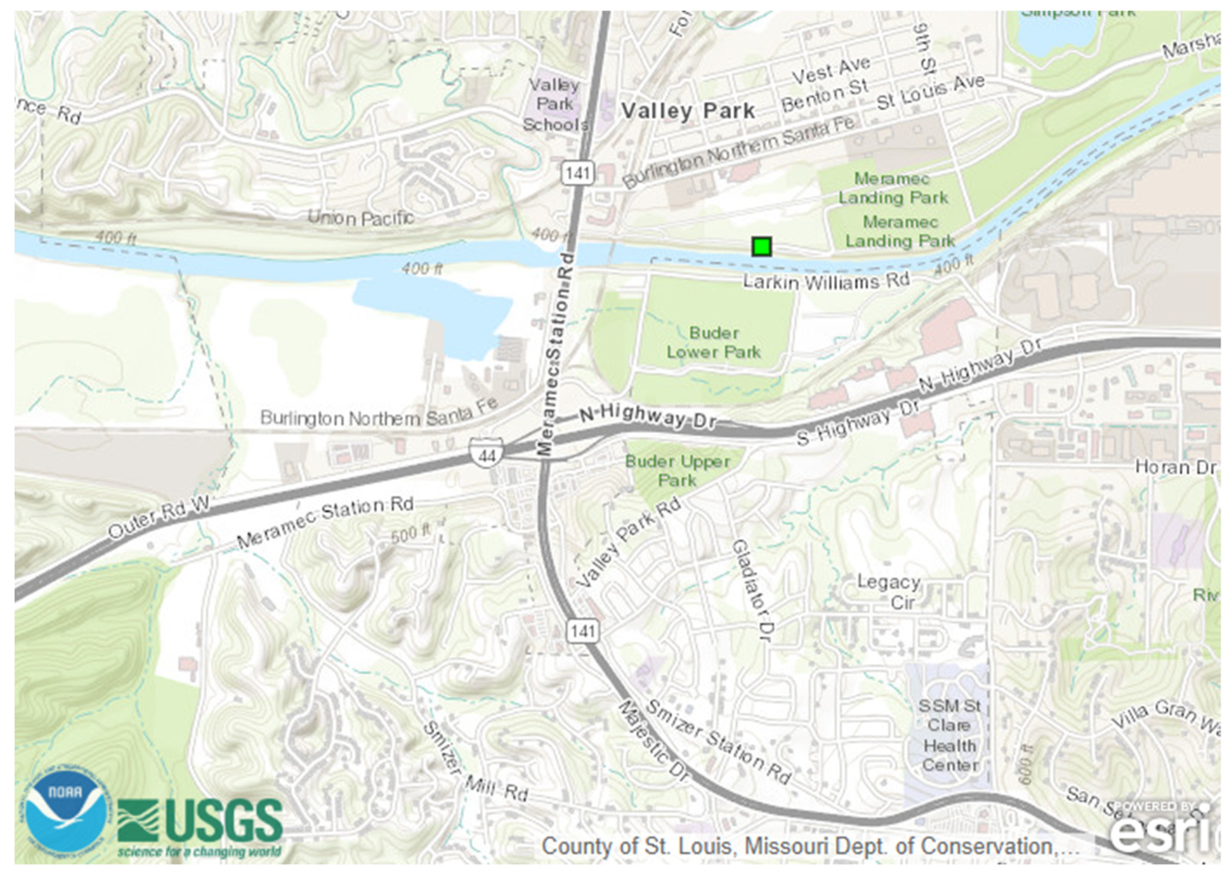
The Meramec River at the intersection of Route 141 and Interstate I-44 at Valley Park, St. Louis County, MO was selected for this research. This location experiences heavy traffic flow [39] and has been impacted by flood events in recent years. The gauge height predictions at this location are developed by the advanced hydrologic prediction service (AHPS), managed by the National Weather Service (NWS), and are provided on the U.S. Geological Survey (USGS) website. These predictions are based on a physical model, developed from digital elevation maps, weather, and other geophysical properties of the given region. These predictions are 6 hours apart and are not useful for transportation networks. Further, physical models cannot be generalized and have to be developed from scratch for each new region. Therefore, there is an opportunity to develop a model with improved prediction time period, accuracy, and generalizability.
The objective of the study is to develop a methodology to predict gauge height and the uncertainty associated with the prediction. The proposed model is data driven and uses historical gauge height data from 15 May 2016 5 PM onward until 1 September 2019 4 PM for the Meramec River in Valley Park, MO. The paper also discusses the future work of incorporating gauge height data into the Flood Inundation Mapper (FIM) tool developed by the United States Geological Survey (USGS), which can then generate future flood profiles for the given region.
2. Materials and Methods
2.1. LSTM Network
A neural network is an artificial intelligence technique based on the functioning of the human brain. The basic unit of a neural network is an “artificial neuron.” For each training sample, the neural network predicts an outcome and then adjusts the weights based on the error. Once trained, this network can be used for prediction on a new data sample (x*). Thus, a neural network represents a function that maps the input variables to the outputs. The predictions from a neural network for a new data sample can be represented as below.
y*= fw x*
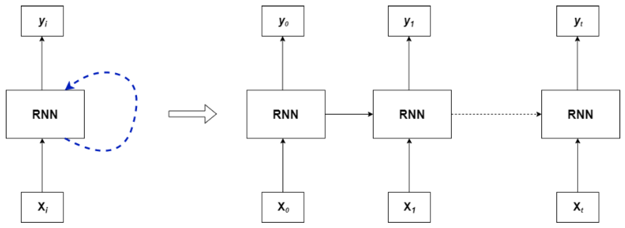
One shortcoming of traditional neural networks is that they cannot retain temporal information. To account for this shortcoming recurrent neural networks (RNN) were introduced. This network consists of loops that help in retaining information from previous time steps.
A simple representation of a recurrent neural network can be seen in the Figure 1. At a given time “I,” the network makes a prediction (yi) based on the input data (Xi) in a loop and the information is passed from the previous steps to the current steps. The information from the first time step is passed to the next time step and so on. This structure can make this algorithm effective for time series forecasting. The input vector (X0) consists of inputs x0, x1, ….xm where “m” is known as the lookback. In other words, RNN looks at the past “m” data samples to make prediction for the current time step. A short coming identified with this approach is not being able to retain information in the long term. Therefore, as the steps increases, the information diminishes.
Gauge height prediction is a time-series forecasting problem that uses data for the past (n − 1) time steps to predict the gauge height for the nth step. Based on the literature review, we observed the increasing affinity toward using deep learning techniques for complicated problems, especially LSTM networks when working with time series forecasting.
Deep learning is an advanced form of a neural networks that uses an increased number of layers and layer types to better model complex systems and interactions. Traditional neural networks cannot retain temporal information, so recurrent neural networks were introduced where previous time step information is used. LSTMs are a deep learning version of recurrent neural networks that are capable of retaining longer term information. LSTM cells remove or add information regulated by the use of gates along with vector addition and multiplication to change the data.
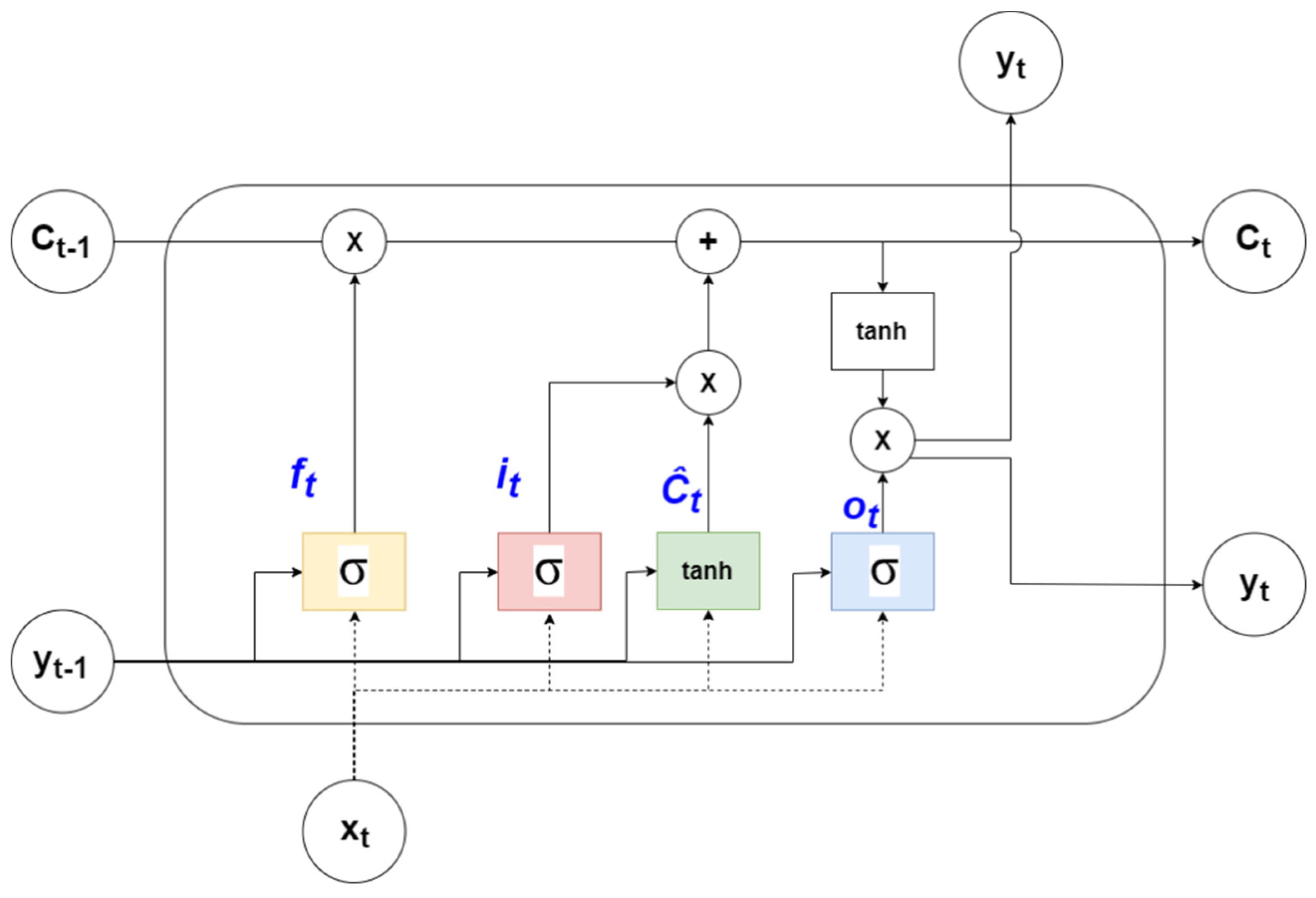
The input vector for the model is defined as X = {x1,….xn} and output vector, Y = {y1,…..,yn}. The gates consist of a sigmoid neural network layer and a point wise multiplication operator. A value of one indicates letting through all data while a value of zero does not allow any of the data to be used. The first gate layer (the “forget” gate layer, represented in “yellow” in Figure 2) takes output from the previous step (yt − 1) and current input (xt) and outputs a value between 0 and 1, indicating how much information is to be passed on. The output from the “forget” gate is represented by ft in Equation (2), where matrices U and W contain weights and recurrent connections respectively.
ft = σ(xt Uf + yt − 1 Wf)
The next step is identifying the information that needs to be stored. A sigmoid layer is once again used to decide which values to update. A tanh layers then generates the new values to be added to the cell state. The corresponding equations for the sigmoid and the tanh layers are shown in Equations (3) and (4).
it = σ(xt Ui + yt − 1 Wi)
Ĉt = tanh (xt Ug + yt − 1 Wg)
The key component of an LSTM cell is the line at the top known as the cell state (Ct) which has minor interactions with rest of the components. The old state (Ct − 1) is multiplied by ft to allow for the possible “forgetting” of the corresponding information. In the next step, the product of it and Ĉt is added to provide new information to the cell state as shown in the Equation (5).
Ct = ft Ct − 1 + it Ĉt
The final layer in an LSTM cell is the output layer that decides the forecast for the current time step. A sigmoid layer and a tanh layer are used to generate the output (yt) as shown in Equations (6) and (7).
ot = σ(xt Uo + yt − 1 Wo)
yt = tanh(Ct) × ot
2.2. Performamnce Metrics
Mean absolute error (MAE) and root-mean square error (RMSE) are the different statistical measures used to quantify the capabilities of the prediction models. MAE represents the average of all the errors between individual predictions () and observation data (yi) values and RMSE measures square root of the mean of the squared errors. Lower values indicate a better model fit for the data for both the metrics. With RMSE, the errors are squared before the average, therefore, prioritizes larger errors. In situations where larger differences can affect the model, RMSE can be a better evaluation measure, otherwise MAE is more appropriate.
2.3. Uncertainty Modeling
For inputs X = {x1,….xn} and outputs Y = {y1,…..,yn}, the resulting function developed by the forecasting algorithm is given by Y = fω(X), where “ω” represents the parameters of the algorithm. In this case, “ω” represents the weights and bias of the LSTM network. With Bayesian modeling, a prior distribution of the model parameters p(ω) is assumed. The corresponding likelihood distribution is defined by p(y|x, ω ). A posterior distribution is then evaluated after observing the data using Bayes’ theorem as given in Equation (10).
The most probable output parameters given our input data is calculated using Equation (10). The output prediction interval for a new input(x*) can then be calculated by integrating the output (y*) on all the values of “ω” [36].
p(y*|x*,X,Y) = ∫ p(y*| fω (x*), ω) p(ω|X,Y) dω
This integration is known as marginal likelihood estimation. This can be performed on simpler forecasting models, but as the number of parameters increases, it becomes computationally expensive. In such situations, an effective approximation technique is required. A probabilistic interpretation of deep learning models can be developed by inferring the distribution over the model’s weights. Variational inference is the approximation technique used to make the posterior calculation tractable. Dropout is one of the most popular regularization techniques used for approximation of Bayesian inference [36].
The uncertainty in Bayesian neural networks comes from the variation in model parameters. With dropout and other regularization techniques, noise is applied in the input or feature space, either adding noise directly to the inputs or dropping out values in the network layers. This noise can be transformed from feature space to parameter space.
To estimate the uncertainty in prediction for input X, the forecasting process with variation is repeated several times (T). The average of these predictions is used to calculate the uncertainty. The posterior mean (m) and uncertainty (c) are given by the Equations (12) and (13), where fi(x) represents the network in each iteration and “p” represents the prior distribution of the network parameters.
Stochastic regularization techniques are used to estimate Bayesian inference. In this research, a technique with random data sub-sequencing is introduced for uncertainty estimation. This proposed methodology has the advantage of not using dropout or introducing error to the inputs. For each iteration, a subset (X = xm, ….., xn) of the original training data (X = x1, ….., xn) is selected. The value of “m” or the starting point of the subset is randomly generated from a set of values, a larger range of these values results in a larger variation allowing for the control of the uncertainty estimates. Finally, the three different techniques adding input noise, dropout and data sub-selection are compared to identify the better model for this problem.
2.4. Quality of Uncertainty
Uncertainty area, empirical coverage and the mean performance metrics are used to compare the different uncertainty estimation techniques. Uncertainty area is defined as the total area covered by 90% uncertainty interval whereas empirical coverage indicates how many of the predictions are captured in the uncertainty interval.
2.5. Data
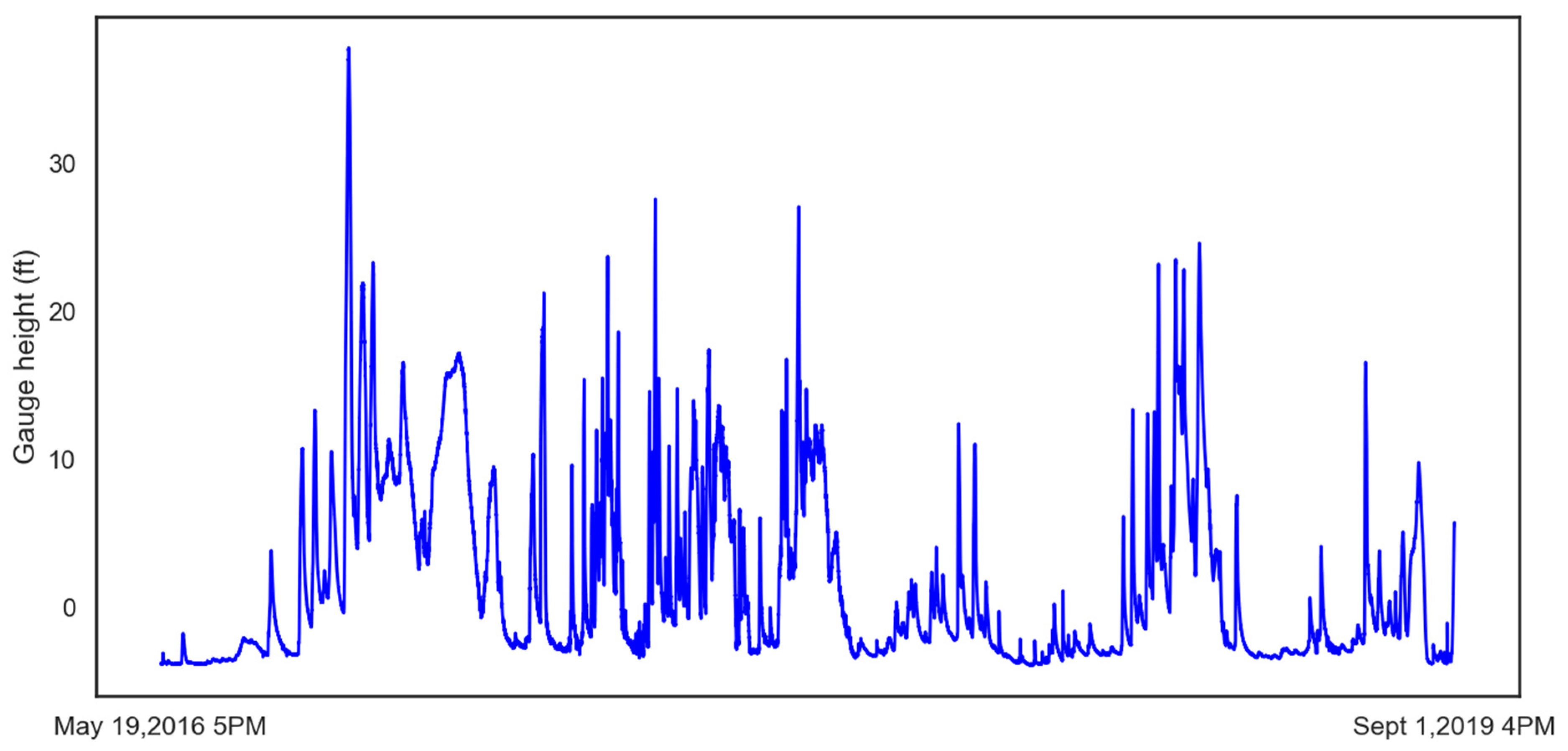
The historical gauge height data used to train the LSTM was obtained from the USGS. The U.S. Army Corps of Engineers – St. Louis District, operate the Valley Park site (Figure 3). The 15-minute time interval data for stage flow at the site is available from 15 May 2016 5 PM onward until 1 September 2019 4 PM. This gives 113,994 samples that when plotted give insight to the number and degree of flood events at that location as shown in Figure 4. The flood stage for this location is 16 ft., and major flood stage is above 25 ft.
3. Results
In this research three evaluations are presented: (1) Developing and comparison of statistical and deep learning models for gauge height prediction, (2) evaluating the effect of dropout on the LSTM performance, and (3) comparison of different uncertainty estimation techniques. To ensure a relevant comparison, the validation of the models is also presented.
3.1. Comparison of Statistical and Deep Learning for Gauge Height Prediction
ARIMA and an LSTM were compared to identify the best methodology for flood prediction. The 15-minute interval gauge height data at the considered location was available starting 19 May 2016. Therefore, for the model to capture the temporal dynamics and patterns, 80% of the gauge height data was used for training (19 May 2016, 5 PM–4 January 2019, 4:15 PM) and the remaining 20% for testing (4 January 2019, 4:30 PM–1 September 2019, 4 PM). “Out of sample” predictions are obtained from 1 September 2019 6 PM to 3 September 2019 12 AM. The parameters of the algorithms are tuned, trained, and tested to evaluate the performance of different algorithms.
ARIMA is a regression model, and all regression models are based on the assumption that the values in the data set are independent of each other. When using regression for time series prediction, it is important to make sure that the data is stationary, meaning that the statistical properties such as variance do not change with time. In ARIMA, “AR” refers to the “autoregressive” component, which is the lag of the stationary series, moving average (MA) captures the lags of the forecast errors and “I” represents the order of differentiation to make the series stationary. The Dickey Fuller test was used to verify that the time-series data were stationary. The resultant p-value for the gauge height data was lower than 0.01 and the test static was −8.527531, thereby allowing us to reject the null hypothesis and conclude that the data is stationary.
The ARIMA (p, d, q) is the model used in this research, where “p” is the autoregressive component, “d” is the number of non-seasonal differences to make the series stationary, and “q” represents the moving average term. Different values of p, d, and q are tested and the results as shown in Table 1. AIC (Akaike Information Criterion) and BIC (Bayesian Information Criterion) are used to evaluate the performance of the different configurations of “p,” ”d,” and “q” [41]. The (p, d, q) values are generated using the Python library “pmdarima.” The model with parameters of (1, 1, 3) gives the lowest AIC and BIC values making it the best choice to compare with the LSTM.
The final architecture for the LSTM is selected through a parameter sweep in Python using the deep learning library, “keras” Different configurations of the architecture elements such as number of hidden layers, width of the hidden layers (number of neurons), batch size, activation functions, and optimizers were tested using “grid search” and “trial and error” approaches. The best performing architecture, which specifies the shape of the output generated, is shown in Table 2. The look back for the model is “90,” meaning it looks at the past 90 values to predict the 91st value. The input layer consisting of 90 neurons takes the input and passes the output onto the layer, which consists of 20 neurons. The output from the LSTM layer was passed onto the dense layer generating a single output, which is the 91st value or the forecast generated by the model. The other parameters were batch size of 60 and “adam” as the optimizer. The final model consists of 120,501 trainable parameters repeated for 100 epochs.
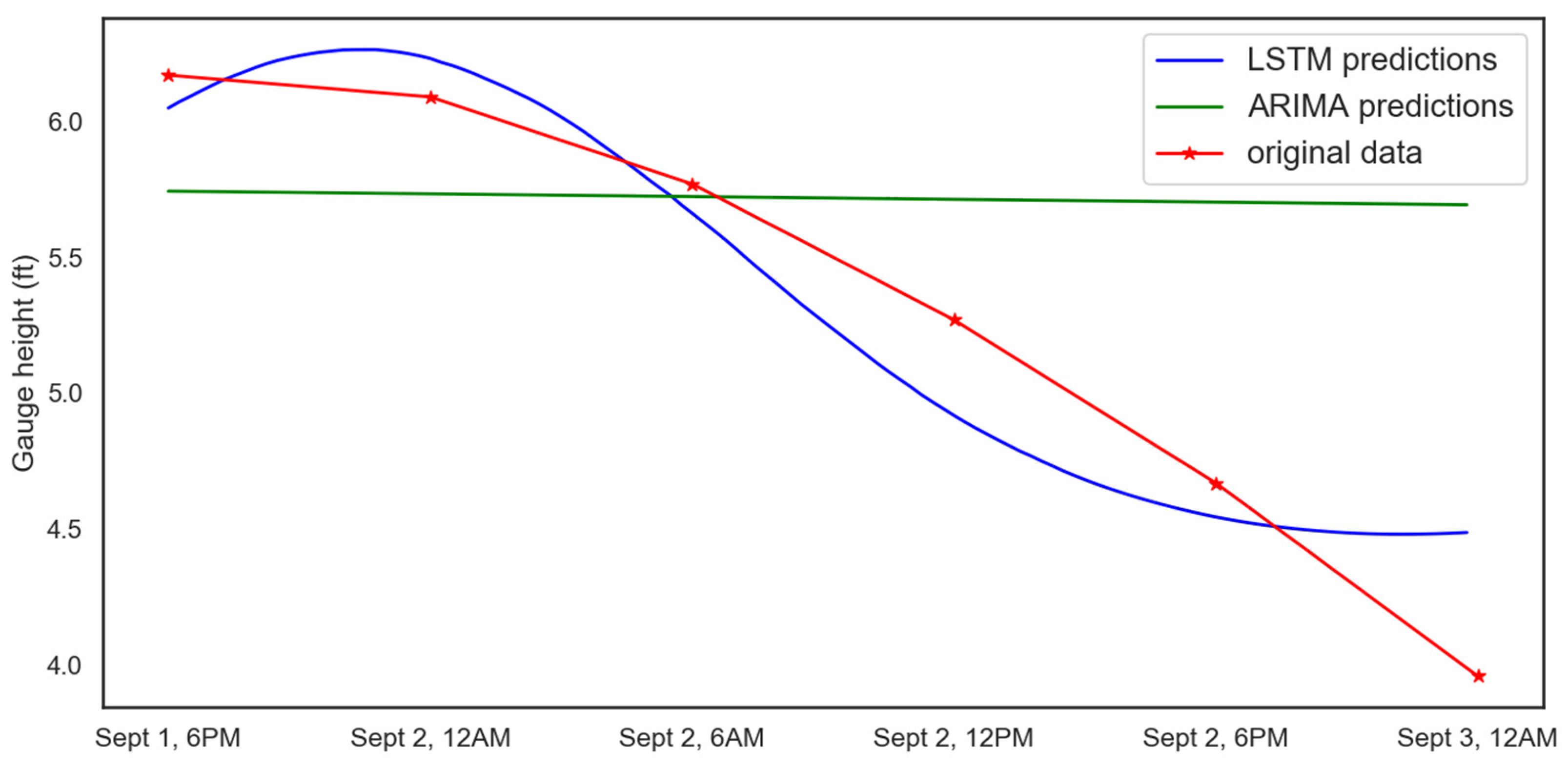
The error in the two prediction methods for the test data are shown in Table 3. Once trained, both the ARIMA and LSTM models were used to make predictions starting at 6 PM on 1 September until 12 AM 3 September. Figure 5 and Table 4 show that the LSTM model performs better at predicting gauge height when compared to ARIMA.
3.2. Effect of Dropout on Model Performance
Monte Carlo dropout is one of the several regularization techniques used to avoid overfitting and improve LSTM performance. The values of a dropout layer range from “0” to “1,” representing the proportion of the nodes from the previous layer removed at random. Dropout was applied during both training for regularization and testing for Bayesian interpretation.
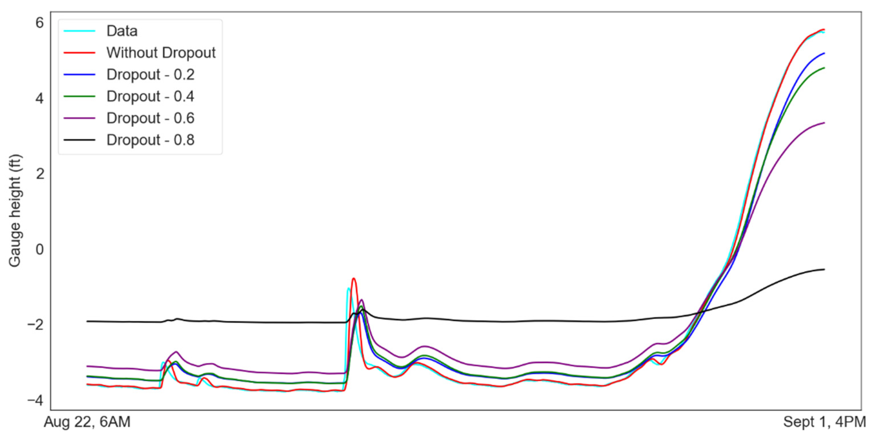
The large data set used for testing makes visualization of the difference between the data challenging. To highlight the differences, Figure 6 shows a small section of the results from 22 August 2019 at 6 AM until 1 September 2019 at 4 PM. The plot shows the effect of different levels of dropout on model performance for the test data. The dropout has a negative impact on the model performance due to its regularization capability. It can be observed that the prediction error increases with an increase in the value of “dropout.” The results are as shown in Table 5. The evaluation metrics were calculated based on the entire testing data.
3.3. Uncertainty Estimation
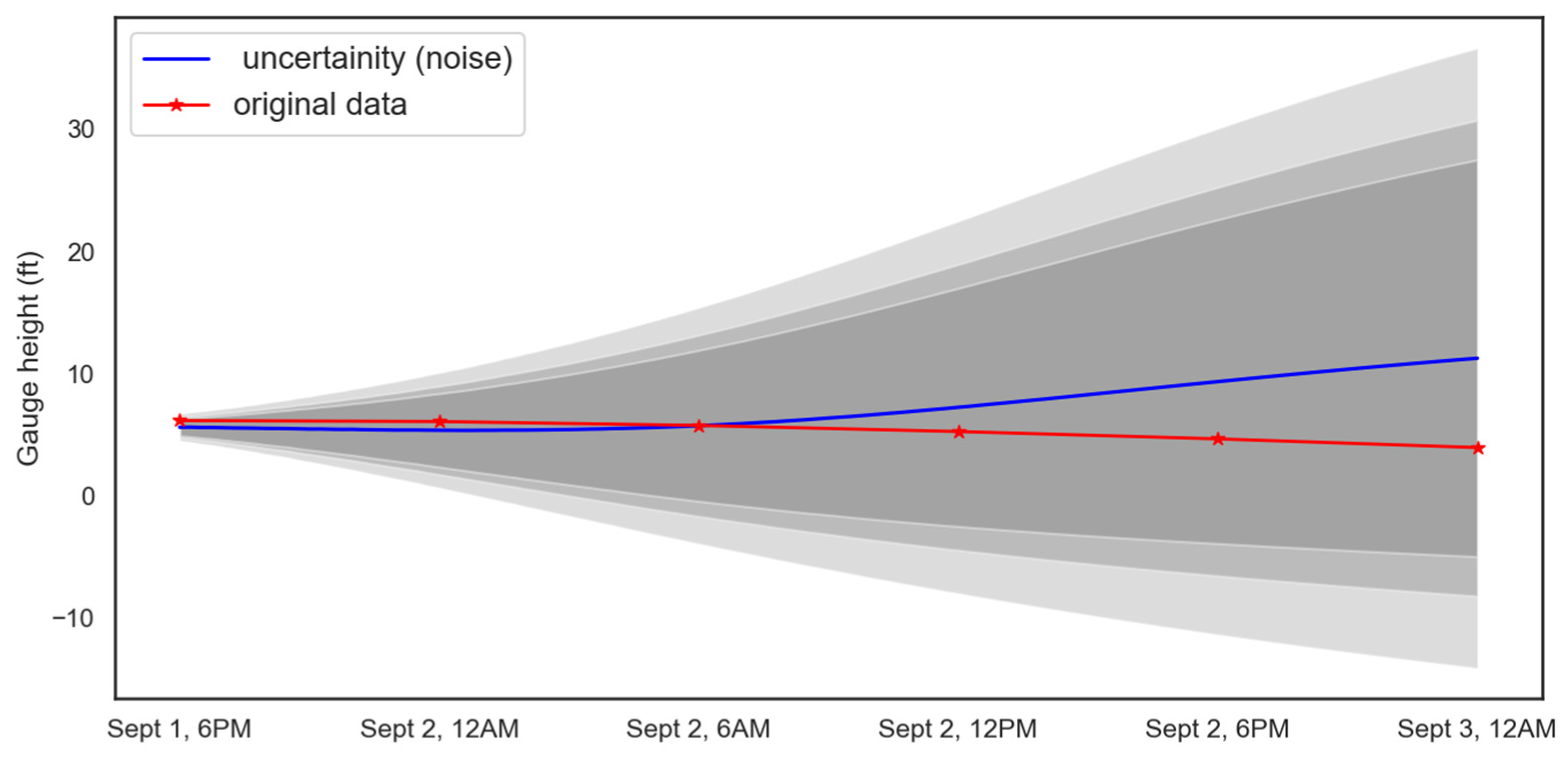
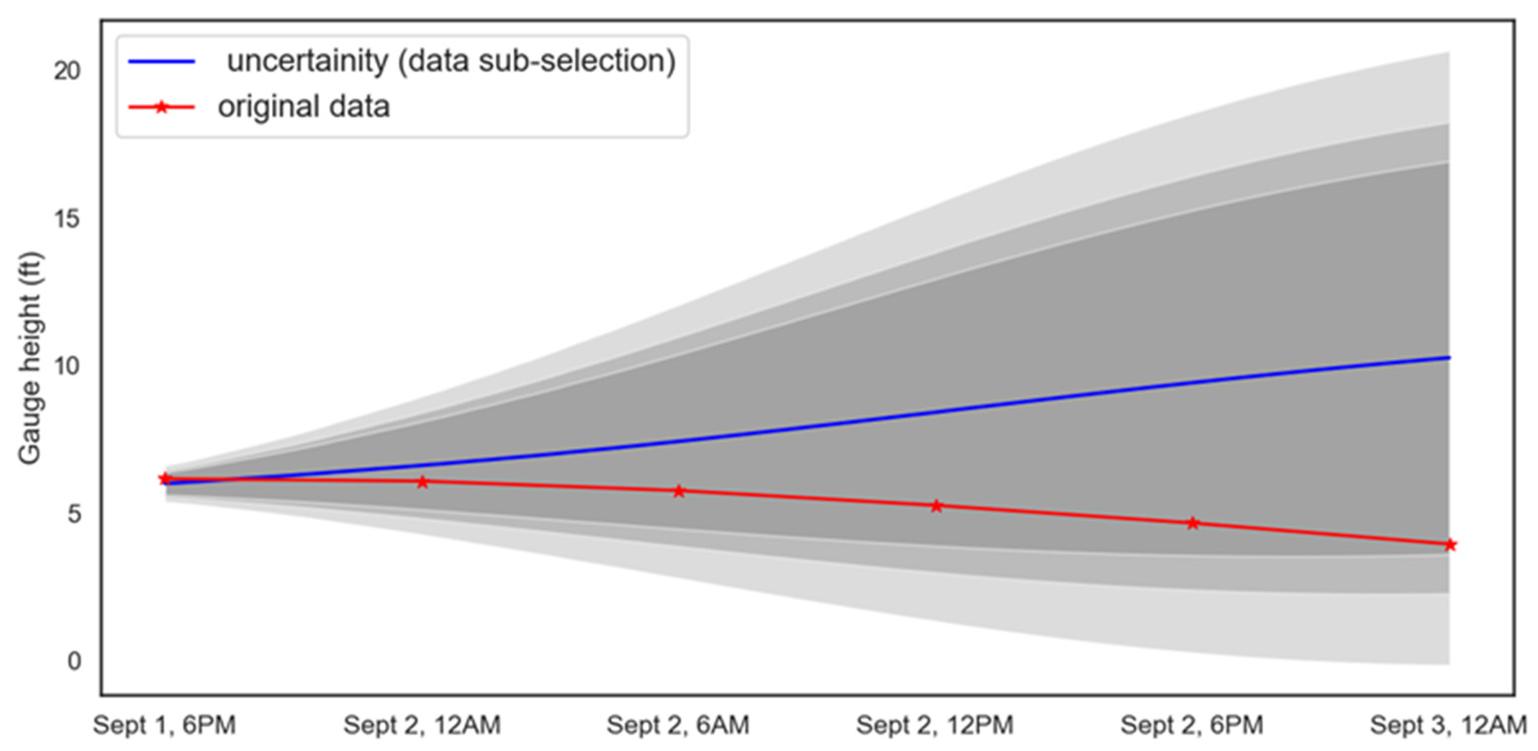
Three different uncertainty estimation techniques were used to analyze the data: data sub-selection, noise, and dropout. Several ranges for data sub-selection were tested, and a range of (S/1000, S/2) performed best and so was used, where S represents the total length of the training data was used to identify the best range for this problem. Ranges of values from (0.1 to 0.8) were used for the dropout layer and a normal distribution of mean “0” and variance between “0.01” and “0.1” for noise were tested. Total of 200 simulations were performed for each model. The final parameters chosen for the models are 0.2 for dropout, a range of +/− 0.1 for noise, and (S/100, 2/2) for data sub-selection. The confidence intervals for dropout are shown in Figure 7, the noise results are given in Figure 8, and the data sub-selection results are given in Figure 9. Each prediction has a certain degree of error associated with it and these predictions used to make further predictions as the model continues to run. As more predictions are made using more predicted values rather than true data points, these error are propagated and build up to cause more uncertainty. This can be seen as an increase in the error bounds and a corresponding loss of accuracy, observed from the Figure 7, Figure 8, Figure 9, Figure 10 and Figure 11. The three different shades indicate 95%, 90%, and 85% intervals starting from light to dark. The 95% confidence intervals were used to compare the performance of the different approaches.
The uncertainty estimation results are as shown in Table 6. The corresponding RMSE, MAE, and uncertainty area are evaluated based on the predicted mean values, which are represented in “blue” in the Figure 7, Figure 8 and Figure 9.
All the models have similar RMSE and MAE values, however; there is a significant difference in the area under the 95% prediction interval. The range of uncertainty values increases with time for all the models. Data sub-selection has the smallest uncertainty area, followed by dropout, and then random noise. The mean predictions for dropout are slightly better than the other models. The range of predictions for 3 September, 12 AM from the three different models are (−9, 29) for dropout, (−12, 33) for noise, and (0, 21) for data sub-selection. While dropout has a slight benefit in accuracy, the data sub-selection model has a much smaller uncertainty area.
3.4. Model Validation
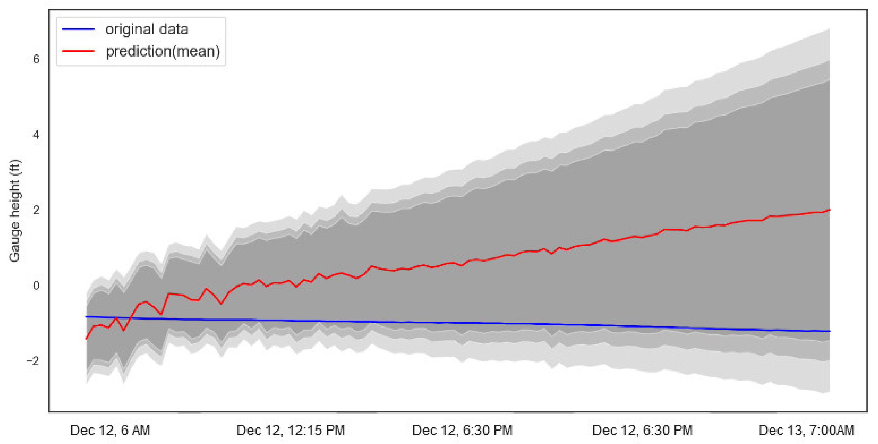
For validation, the LSTM model trained with the May 2016–September 2019 data was used to predict the gauge height for the Meramec River at Valley Park, MO from 6 AM on 12 December 2019 until 7 PM on 13 December 2019. The predictions are shown in Figure 10. During this period, the gauge height is stationary and the model was able to capture all the data values within the 95% confidence interval using data sub-selection method.
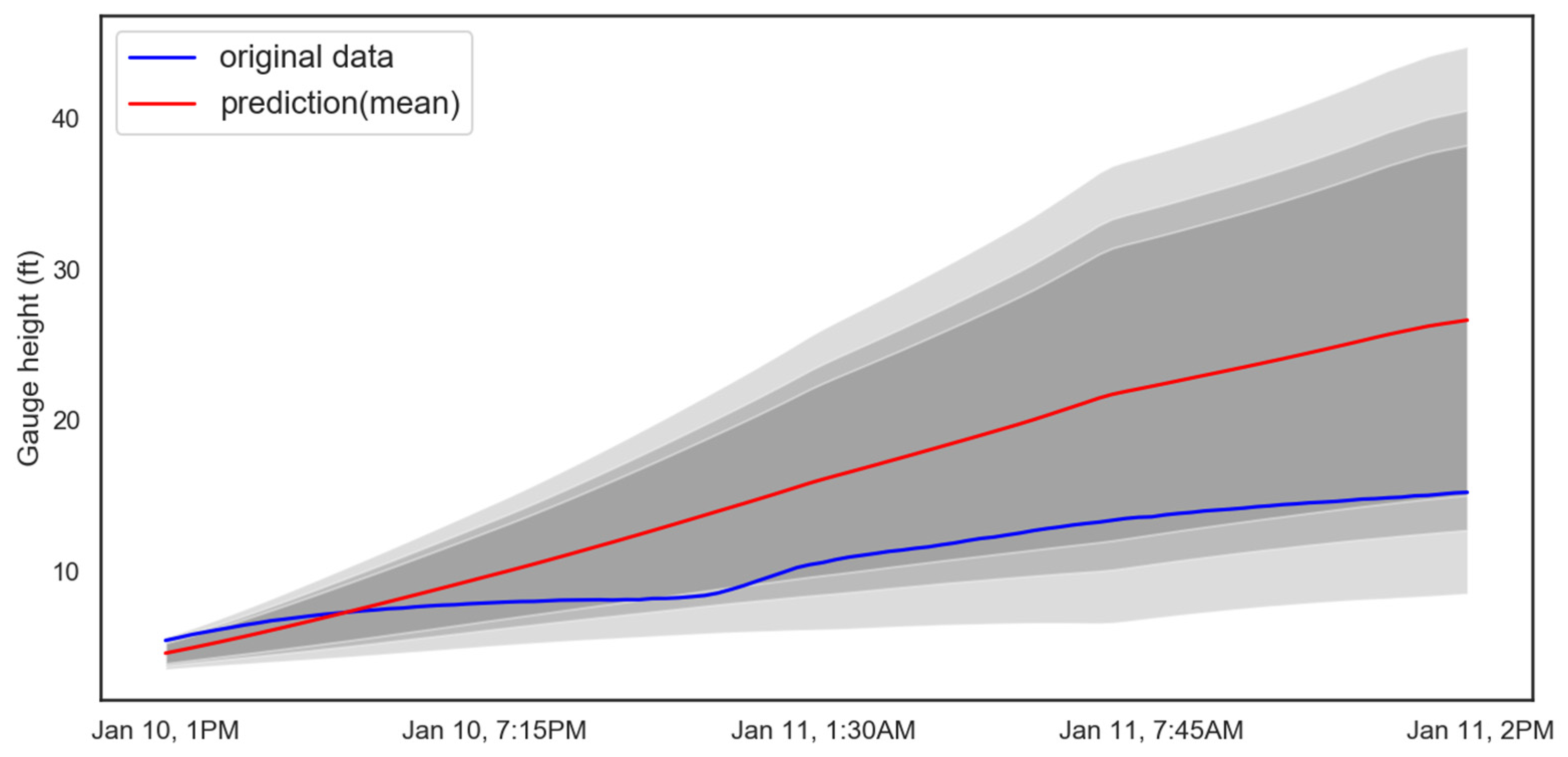
The mean prediction for a day ahead into the future shows a deviation of approximately 2 ft. and a 95% confidence interval range of 8 ft for scenario 1. Further, the model was used to generate the forecasts when the gauge height is increasing and the corresponding results can be seen in Figure 11. The predicted mean during validation shows little deviation from the actual data, showing the capability of the model for real time gauge height predictions. The lead-time from the above figure can be observed to be 1 day and 1 hour. The model gives the flexibility to adjust the lead-time. Therefore, it provides the ability to modify according to the corresponding user’s requirements.
4. Discussion
Deep learning models are based on the assumption that the layers and activation function would be able to capture the seasonality and trend within the data. Gauge height prediction is a complex problem as it is an observation from an intricate system consisting of weather and geophysical elements. Obtaining all the information is data intensive and in most situations, the data is not available, inconsistent, or available only for a short period. Therefore, deep learning prediction model is an ideal solution for such problems.
The LSTM was able to predict gauge height more accurately than ARIMA or physics-based models currently used by the USGS, likely because of its ability to capture long-term temporal dynamics. Because of the large time frame considered in the data set, the LSTM is better designed to capture small variation in the predictions than the ARIMA model. The moving average used by the ARIMA model seems to discourage variation, making the ARIMA model less able to capture the rapid change in water level found in the out of sample data. One of the challenges with predictions from deep learning models is the uncertainty quantification. This can be addressed by comparing the uncertainty estimates from different regularization techniques. Dropout is explored as a method for regulating the LSTM model, but a direct relationship between the error and the dropout value was found, showing that in this application dropout did not perform well. The data sub-selection method was shown to provide a better performance when used in Bayesian inferencing. Data sub-selection led to less uncertainty than both the dropout method and the random noise method. The predicted gauge heights were validated by comparing the results of the uncertainty analysis to the actual values recorded at this location from 12 December 2019 6 AM until 13 December 2019 7 AM using the same model architecture as was used for dropout testing and the uncertainty analysis. This demonstrates that the LSTM model can be used with dropout and other uncertainty estimation techniques to improve the architecture and reduce the prediction uncertainty.
River gauge height is currently used by USGS for flood inundation mapping, but inconsistency in the data available at different locations is a challenge. Many sites are operated by different organizations, resulting in variation in the type of data (weather data, gauge height, and discharge) and the time step for the data recordings. For example, two gauges in Saint Louis, the one on Meramec river in Valley Park, MO and the another one in downtown Saint Louis in the Mississippi river, are both operated by the United States Army Corps of Engineers–St. Louis District but have recordings time steps of 15 minutes and 1 hour respectively. This inconsistency results in the need to train the model for each gauge separately. The methodology presented here can identify the appropriate model in less time and with fewer resources.
The objective of the research was to develop a methodology to predict gauge height more accurately and develop an uncertainty measure to identify the quality of those predictions. The uncertainty interval can be controlled by regulating the variability being introduced to the data or the model. It should be noted that the model architecture was not changed when introducing these variations. This was done to show that existing models could be used to develop uncertainty estimates. We can further improve the estimates by optimizing the model architecture for each variation.
In the context of floods, accurate gauge height predictions can be used to develop the relevant flood mapping and identify the possible damage in the future. This can be helpful for emergency response and other applications to preemptively relocate people, close roads, and take other precautionary measures to save lives. The 3-dimensional digital elevations models published by the USGS can be used to develop the flood mapping for a given region using software such as ArcGIS and QGIS based on the gauge height predictions generated by the current model. The USGS recently published “Flood Inundation Mapper” (FIM), a tool that provides this type of flood mapping for a given region for a given gauge height. There are a limited number of locations currently included in FIM (Figure 12), but new regions are being added every month. As this resource becomes more available, it can become a useful tool to be integrated along with the gauge height prediction to generate the future flood mapping for a given region.
One of the major reasons for deaths during floods is that people underestimating the amount of water and driving into the flooded roads. The use of this method for flood prediction not only gives a more accurate prediction, but also provides gauge height prediction at a smaller interval than currently being used. This methodology can be integrated with road network models to identify the flooded roads ahead of time to preemptively close roads, put up signs and evaluate alternative routes for the travelers.
Author Contributions
This research is a cooperative effort between the authors. V.G., S.C., and S.L. all contributed to the conceptualization, formal analysis, investigation, methodology, and validation of the work. All three authors also worked to review and edit the document. V.G. and S.C. wrote the original draft. S.L. and S.C. performed the funding acquisition, project administration, and supervision of the project. S.C. procured the computing resources for the work. V.G. wrote the necessary software and created the visualizations included in the work. All authors have read and agreed to the published version of the manuscript.
Funding
This research was funded by the Missouri Department of Transportation; grant number TR201912 and the Mid-America Transportation Center, grant number 25-1121-0005-130.
Conflicts of Interest
The authors declare no conflict of interest.
References
- Sieg, T.; Schinko, T.; Vogel, K.; Mechler, R.; Merz, B.; Kreibich, H. Integrated assessment of short-term direct and indirect economic flood impacts including uncertainty quantification. PLoS ONE 2019, 14, e0212932. [Google Scholar] [CrossRef] [PubMed] [Green Version]
- Faiz, M.A.; Liu, D.; Fu, Q.; Qamar, M.; Dong, S.; Khan, M.; Li, T. Complexity and trends analysis of hydrometeorological time series for a river streamflow: A case study of Songhua River Basin, China. River Res. Appl. 2017, 34, 101–111. [Google Scholar] [CrossRef]
- Pitt, M. Learning lessons from the 2007 floods. In The Pitt Review; Cabinet Office: London, UK, 2008. [Google Scholar]
- Mosavi, A.; Ozturk, P.; Chau, K.-W. Flood Prediction Using Machine Learning Models: Literature Review. Water 2018, 10, 1536. [Google Scholar] [CrossRef] [Green Version]
- Cea, L.; Garrido, M.; Puertas, J. Experimental validation of two-dimensional depth-averaged models for forecasting rainfall–runoff from precipitation data in urban areas. J. Hydrol. 2010, 382, 88–102. [Google Scholar] [CrossRef]
- Costabile, P.; Macchione, F. Enhancing river model set-up for 2-D dynamic flood modelling. Environ. Model. Softw. 2015, 67, 89–107. [Google Scholar] [CrossRef]
- Liang, X.; Lettenmaier, D.P.; Wood, E.; Burges, S.J. A simple hydrologically based model of land surface water and energy fluxes for general circulation models. J. Geophys. Res. Space Phys. 1994, 99, 14415. [Google Scholar] [CrossRef]
- Costabile, P.; Costanzo, C.; Macchione, F. Two-dimensional numerical models for overland flow simulations. River Basin Manag. V 2009, 124, 137–148. [Google Scholar]
- Fraga, I.; Cea, L.; Puertas, J. MERLIN: A flood hazard forecasting system for coastal river reaches. Nat. Hazards 2020, 100, 1171–1193. [Google Scholar] [CrossRef]
- Honert, R.V.D.; McAneney, J. The 2011 Brisbane Floods: Causes, Impacts and Implications. Water 2011, 3, 1149–1173. [Google Scholar] [CrossRef] [Green Version]
- Bout, B.; Jetten, V. The validity of flow approximations when simulating catchment-integrated flash floods. J. Hydrol. 2018, 556, 674–688. [Google Scholar] [CrossRef]
- Costabile, P.; Macchione, F.; Natale, L.; Petaccia, G. Flood mapping using LIDAR DEM. Limitations of the 1-D modeling highlighted by the 2-D approach. Nat. Hazards 2015, 77, 181–204. [Google Scholar] [CrossRef]
- Sopelana, J.; Cea, L.; Ruano, S. A continuous simulation approach for the estimation of extreme flood inundation in coastal river reaches affected by meso- and macrotides. Nat. Hazards 2018, 93, 1337–1358. [Google Scholar] [CrossRef]
- Bellos, V.; Tsakiris, G. A hybrid method for flood simulation in small catchments combining hydrodynamic and hydrological techniques. J. Hydrol. 2016, 540, 331–339. [Google Scholar] [CrossRef]
- Hernández, F.; Liang, X. Hybridizing Bayesian and variational data assimilation for high-resolution hydrologic forecasting. Hydrol. Earth Syst. Sci. 2018, 22, 5759–5779. [Google Scholar] [CrossRef] [Green Version]
- Ferraro, D.; Costabile, P.; Costanzo, C.; Petaccia, G.; Macchione, F. A spectral analysis approach for the a priori generation of computational grids in the 2-D hydrodynamic-based runoff simulations at a basin scale. J. Hydrol. 2020, 582, 124508. [Google Scholar] [CrossRef]
- Adamowski, J.; Chan, H.F.; Prasher, S.O.; Ozga-Zielinski, B.; Sliusarieva, A. Comparison of multiple linear and nonlinear regression, autoregressive integrated moving average, artificial neural network, and wavelet artificial neural network methods for urban water demand forecasting in Montreal, Canada. Water Resour. Res. 2012, 48, 1–14. [Google Scholar] [CrossRef]
- Valipour, M.; Banihabib, M.E.; Behbahani, S.M.R. Comparison of the ARMA, ARIMA, and the autoregressive artificial neural network models in forecasting the monthly inflow of Dez dam reservoir. J. Hydrol. 2013, 476, 433–441. [Google Scholar] [CrossRef]
- Bermúdez, M.; Cea, L.; Puertas, J. A rapid flood inundation model for hazard mapping based on least squares support vector machine regression. J. Flood Risk Manag. 2019, 12, e12522. [Google Scholar] [CrossRef] [Green Version]
- Thompson, S.A. Hydrology of Water Management; CRC Press: Boca Raton, FL, USA, 2017. [Google Scholar]
- Mekanik, F.; Imteaz, M.; Gato-Trinidad, S.; Elmahdi, A. Multiple regression and Artificial Neural Network for long-term rainfall forecasting using large scale climate modes. J. Hydrol. 2013, 503, 11–21. [Google Scholar] [CrossRef]
- Abbot, J.; Marohasy, J. Input selection and optimisation for monthly rainfall forecasting in Queensland, Australia, using artificial neural networks. Atmos. Res. 2014, 138, 166–178. [Google Scholar] [CrossRef]
- Ortiz-Garcia, E.; Salcedo-Sanz, S.; Casanova-Mateo, C. Accurate precipitation prediction with support vector classifiers: A study including novel predictive variables and observational data. Atmos. Res. 2014, 139, 128–136. [Google Scholar] [CrossRef]
- Kim, S.Y.; Matsumi, Y.; Pan, S.; Mase, H. A real-time forecast model using artificial neural network for after-runner storm surges on the Tottori coast, Japan. Ocean Eng. 2016, 122, 44–53. [Google Scholar] [CrossRef]
- Dineva, A.; Várkonyi-Kóczy, A.R.; Tar, J.K. Fuzzy expert system for automatic wavelet shrinkage procedure selection for noise suppression. In Proceedings of the IEEE 18th International Conference on Intelligent Engineering Systems INES 2014, Tihany, Hungary, 3–5 July 2014; pp. 163–168. [Google Scholar]
- Asanjan, A.A.; Yang, T.; Hsu, K.; Sorooshian, S.; Lin, J.; Peng, Q. Short-Term Precipitation Forecast Based on the PERSIANN System and LSTM Recurrent Neural Networks. J. Geophys. Res. Atmos. 2018, 123, 543. [Google Scholar]
- Hu, C.; Wu, Q.; Li, H.; Jian, S.; Li, N.; Lou, Z. Deep Learning with a Long Short-Term Memory Networks Approach for Rainfall-Runoff Simulation. Water 2018, 10, 1543. [Google Scholar] [CrossRef] [Green Version]
- Zhang, D.; Martinez, N.; Lindholm, G.; Ratnaweera, H. Manage Sewer In-Line Storage Control Using Hydraulic Model and Recurrent Neural Network. Water Resour. Manag. 2018, 32, 2079–2098. [Google Scholar] [CrossRef]
- Kratzert, F.; Klotz, D.; Brenner, C.; Schulz, K.; Herrnegger, M. Rainfall–runoff modelling using long short-term memory (LSTM) networks. Hydrol. Earth Syst. Sci. 2018, 22, 6005–6022. [Google Scholar] [CrossRef] [Green Version]
- Ogunmolu, O.; Gu, X.; Jiang, S.; Gans, N. Nonlinear Systems Identification Using Deep Dynamic Neural Networks. arXiv 2016, arXiv:1610.01439. [Google Scholar]
- Dietz, R.; Casavant, T.; Scheetz, T.; Braun, T.; Andersland, M. Modeling the impact of run-time uncertainty on optimal computation scheduling using feedback. In Proceedings of the 1997 International Conference on Parallel Processing (Cat. No.97TB100162), Bloomington, IL, USA, 11–15 August 1997; pp. 481–488. [Google Scholar]
- Zhu, L.; Laptev, N. Deep and Confident Prediction for Time Series at Uber. In Proceedings of the 2017 IEEE International Conference on Data Mining Workshops (ICDMW), New Orleans, LA, USA, 18–21 November 2017; pp. 103–110. [Google Scholar]
- Paisley, J.; Blei, D.M.; Jordan, M.I. Variational Bayesian inference with stochastic search. Int. Conf. Mach. Learn. 2012, 2, 1367–1374. [Google Scholar]
- Kingma, D.P.; Welling, M. Auto-encoding variational bayes. Int. Conf. Learn. Represent. 2014, 1–14. Available online: https://dare.uva.nl/search?identifier=cf65ba0f-d88f-4a49-8ebd-3a7fce86edd7 (accessed on 21 March 2020).
- Hernández-Lobato, J.M.; Adams, R.P. Probabilistic backpropagation for scalable learning of Bayesian neural networks. Int. Conf. Mach. Learn. 2015, 3, 1861–1869. [Google Scholar]
- Gal, Y.; Ghahramani, Z. Dropout as a Bayesian approximation: Representing model uncertainty in deep learning. Int. Conf. Mach. Learn. 2016, 3, 1651–1660. [Google Scholar]
- Hernández-Lobato, J.M.; Li, Y.; Rowland, M.; Hernández-Lobato, D.; Bui, T.D.; Ttarner, R.E. Black-Box α-divergence minimization. Int. Conf. Mach. Learn. 2016, 4, 2256–2273. [Google Scholar]
- Li, Y.; Gal, Y. Dropout Inference in Bayesian Neural Networks with Alpha-divergences. Conf. Mach. Learn. 2017, 5, 3219–3232. [Google Scholar]
- Missouri Department of Transportation. 2015 St. Louis District Traffic Volume and Commercial Vehicle Count Map. Available online: https://www.modot.org/sites/default/files/documents/2015._Traffic_SL_06212016%5B1%5D.pdf (accessed on 9 March 2020).
- USGS Water Data for the Nation. Available online: https://waterdata.usgs.gov/nwis (accessed on 17 December 2019).
- Spanos, A. Akaike-type criteria and the reliability of inference: Model selection versus statistical model specification. J. Econ. 2010, 158, 204–220. [Google Scholar] [CrossRef]
- Flood Inundation Mapper. Available online: https://fim.wim.usgs.gov/fim/ (accessed on 17 December 2019).
Figure 1.
Recurrent neural network.

Figure 2.
Long short-term memory networks (LSTM) cell.

Figure 3.
Gauge location in Meramec River [40].
Figure 3.
Gauge location in Meramec River [40].

Figure 4.
Gauge height data used for training and testing.

Figure 5.
Out of sample prediction from ARIMA and LSTM.

Figure 6.
Test predictions with variation in dropout.

Figure 7.
Out of sample prediction uncertainty estimation with “dropout.”

Figure 8.
Out of sample prediction uncertainty estimation with “noise.”

Figure 9.
Out of sample prediction uncertainty estimation with “data sub-selection.”

Figure 10.
Forecasts with uncertainty estimations.

Figure 11.
Forecasts of river level with uncertainty with increasing gauge.

Figure 12.
Available flood mapping locations in Flood Inundation Mapper (FIM) [42].
Figure 12.
Available flood mapping locations in Flood Inundation Mapper (FIM) [42].


Table 1.
Autoregressive integrated moving average (ARIMA) parameter selection results.
| Parameters | AIC | BIC |
|---|---|---|
| (0,1,1) | −258,152.156 | −258,123.893 |
| (0,1,0) | −248,137.561 | −248,118.719 |
| (1,1,0) | −266,952.850 | −266,924.587 |
| (2,1,2) | −303,596.995 | −303,540.467 |
| (1,1,2) | −303,594.450 | −303,547.344 |
| (2,1,1) | −303,212.512 | −303,165.405 |
| (3,1,2) | −303,479.822 | −303,413.873 |
| (2,1,3) | −303,605.067 | −303,539.118 |
| (1,1,3) | −303,607.796 | −303,551.268 |
| (0,1,3) | −278,432.067 | −278,384.961 |
| (1,1,4) | −303,601.785 | −303,535.836 |
| (0,1,2) | −270,281.324 | −270,243.639 |
| (0,1,4) | −283,568.922 | −283,512.394 |
| (2,1,4) | −303,603.607 | −303,528.236 |
Table 2.
LSTM architecture.
| Layers | Output |
|---|---|
| Input Layer | (None,1,90) |
| LSTM Layer | (None,20) |
| Dense Layer | (None,1) |
| Forecasts | 1 |
Table 3.
Testing data for LSTM and ARIMA.
| Model | RMSE | MAE |
|---|---|---|
| ARIMA | 2.0813 | 1.9442 |
| LSTM | 1.9558 | 1.7010 |
Table 4.
Root mean square error and mean absolute error results of LSTM and ARIMA on “Out of sample” predictions.
Table 4.
Root mean square error and mean absolute error results of LSTM and ARIMA on “Out of sample” predictions.
| Model | RMSE | MAE |
|---|---|---|
| ARIMA | 0.8722 | 0.6732 |
| LSTM | 0.3316 | 0.2595 |
Table 5.
LSTM performance with variation in dropout.
| Model | RMSE | MAE |
|---|---|---|
| Without dropout | 0.1965 | 0.1216 |
| Dropout—0.2 | 0.5585 | 0.2817 |
| Dropout—0.4 | 0.8825 | 0.4082 |
| Dropout—0.6 | 1.6377 | 0.8777 |
| Dropout—0.8 | 2.6855 | 1.6808 |
Table 6.
Comparison of uncertainty estimation techniques.
| Model | RMSE | MAE | Uncertainty Area |
|---|---|---|---|
| Dropout | 3.4672 | 2.3763 | 2703.8913 |
| Noise | 3.6540 | 2.5444 | 3039.4859 |
| Data sub-selection | 3.5430 | 2.7603 | 1376.0500 |
© 2020 by the authors. Licensee MDPI, Basel, Switzerland. This article is an open access article distributed under the terms and conditions of the Creative Commons Attribution (CC BY) license (http://creativecommons.org/licenses/by/4.0/).
Share and Cite
MDPI and ACS Style
Gude, V.; Corns, S.; Long, S. Flood Prediction and Uncertainty Estimation Using Deep Learning. Water 2020, 12, 884. https://doi.org/10.3390/w12030884
AMA Style
Gude V, Corns S, Long S. Flood Prediction and Uncertainty Estimation Using Deep Learning. Water. 2020; 12(3):884. https://doi.org/10.3390/w12030884
Chicago/Turabian StyleGude, Vinayaka, Steven Corns, and Suzanna Long. 2020. "Flood Prediction and Uncertainty Estimation Using Deep Learning" Water 12, no. 3: 884. https://doi.org/10.3390/w12030884
Note that from the first issue of 2016, this journal uses article numbers instead of page numbers. See further details here.