Evaluation of Flood Prediction Capability of the WRF-Hydro Model Based on Multiple Forcing Scenarios

Abstract

The Weather Research and Forecasting (WRF)-Hydro model as a physical-based, fully-distributed, multi-parameterization modeling system easy to couple with numerical weather prediction model, has potential for operational flood forecasting in the small and medium catchments (SMCs). However, this model requires many input forcings, which makes it difficult to use it for the SMCs without adequate observed forcings. The Global Land Data Assimilation System (GLDAS), the WRF outputs and the ideal forcings generated by the WRF-Hydro model can provide all forcings required in the model for these SMCs. In this study, seven forcing scenarios were designed based on the products of GLDAS, WRF and ideal forcings, as well as the observed and merged rainfalls to assess the performance of the WRF-Hydro model for flood simulation. The model was applied to the Chenhe catchment, a typical SMC located in the Midwestern China. The flood prediction capability of the WRF-Hydro model was also compared to that of widely used Xinanjiang model. The results show that the three forcing scenarios, including the GLDAS forcings with observed rainfall, the WRF forcings with observed rainfall and GLDAS forcings with GLDAS-merged rainfall, are optimal input forcings for the WRF-Hydro model. Their mean root mean square errors (RMSE) are 0.18, 0.18 and 0.17 mm/h, respectively. The performance of the WRF-Hydro model driven by these three scenarios is generally comparable to that of the Xinanjiang model (RMSE = 0.17 mm/h).

1. Introduction

Flood disaster is one of the common natural disaster, which often causes loss of life and property [1,2]. The risk of extreme floods in large basins of China has been substantially reduced owing to the improvement of flood forecasting skills in recent years [3]. However, flash flood forecasting and prevention of the small and medium catchments (SMCs) remains an urgent problem [4,5]. The flash floods taking place in the SMCs are characterized by short routing time, which makes flood prediction difficult [6]. Additionally, flood simulation and forecasting for SMCs face more challenges due to sparse observation and inadequate information of field data.

Hydrological models have been widely used to forecast floods over the past decades [7,8,9]. According to whether hydrological processes, input-output data and parameters vary spatially, hydrological models can be classified as lumped, semi-distributed and fully distributed models [9,10,11,12]. Currently, these three kinds of hydrological models are all used for flood forecasting in SMCs. In general, the majority of these models are driven by gauge rainfall data; therefore, the leading time (i.e., the time between flood warning and flood peak) predicted by these models is limited by the catchment routing time. However, the leading time can be maximized by the predicted rainfall from the Numerical Weather Prediction (NWP) models [13,14]. Therefore, the coupled meteo-hydrological modeling system is recognized as a powerful tool for flood forecasting and warning [15,16].

The Weather Research and Forecasting (WRF)-Hydro modeling system [17], as a new generation of fully distributed, multi-scale, physical-based hydrometeorological modeling system, is able to simulate floods, hydrological states and spatial distribution of water resources [18,19]. At present, the Noah or Noah-MP Land Surface Model (LSM) as the lower boundary condition of the NWP model [20,21,22] is used as the runoff generation mechanism in the WRF-Hydro model. Compared to the LSM, a hydrological routing module with finer grids is added to represent subsurface lateral flow [23]. It is found that the WRF-Hydro model using assimilated precipitation based on the WRF model yielded satisfactory results for the flood forecasting of ungauged basins [24]. The performances of fully coupled WRF-Hydro modeling system outperformed the WRF-only model [25]. Other studies on the performance and application of this model have been reported both in uncoupled (WRF-Hydro only) and fully coupled methods (i.e., coupling WRF-Hydro and WRF modeling system) [18,24,25,26,27,28].

The WRF-Hydro model requires spatially distributed forcings including air temperature, surface pressure, specific humidity, near-surface wind speed, incoming longwave and shortwave radiation and rainfall [17]. In general, the available observations from gages in information-poor SMCs contain rainfall, pan evaporation and streamflow at the catchment outlet, which are insufficient to drive the model due to lack of the adequate observed forcings. However, the Global Land Data Assimilation System (GLDAS) [29] as reanalysis data and the WRF model outputs as simulated data are able to provide the adequate forcings for these SMCs. Although the observations, GLDAS and WRF outputs are not available, ideal forcings generated by the WRF-Hydro model through some predefined constants (e.g., surface pressure takes 100,000 Pa all the time) and functions (e.g., air temperature ranges from 287 to 293 K in diurnal cycle) can be used to drive itself [17]. Hence, the GLDAS, WRF outputs and ideal forcings are recognized as the meteorological forcings of the WRF-Hydro model for SMCs in this study.

Rainfall is a crucial forcing of the WRF-Hydro model for flood simulation [5,30,31,32]. However, rainfalls from the GLDAS, WRF outputs and ideal forcings may not be suitable for hydrological simulation. Firstly, the GLDAS-derived rainfall fails to capture features of rainfall fields of SMCs due to its temporal and spatial resolutions, 3 h, 0.25° × 0.25° [33,34,35]. Secondly, the WRF-derived rainfall with flexible spatial resolutions is able to describe rain features such as storm center, but sometimes overestimates the rain area and intensity [36,37]. Lastly, the rainfall from the ideal forcings is only a predefined rainfall series (i.e., 25.4 mm/s for first hourly time step and zero thereafter) that cannot be used in real case. In recent years, some data fusion methods such as precipitation merging method [31,38,39,40,41] are normally applied to reduce the error and enhance the reliability of precipitation. In this study, the Successive Corrections Method [42,43,44,45] was used to merge raw rainfall data from the GLDAS and WRF with gauge data, respectively.

The main objective of this study is to identify the suitable forcings and to evaluate the corresponding performances for the WRF-Hydro model under the multiple forcings scenarios based on observed and merged rainfall, GLDAS, WRF outputs and ideal forcings. The model was applied to the Chenhe catchment, a typical semi-humid SMC located in the Midwestern China. Moreover, the well-known Xinanjiang model, which has been widely used in humid and semi-humid region, was adopted to further investigate the flood prediction capability of the WRF-Hydro model.

2. Data and Method

2.1. Study Catchment and Gauge Data

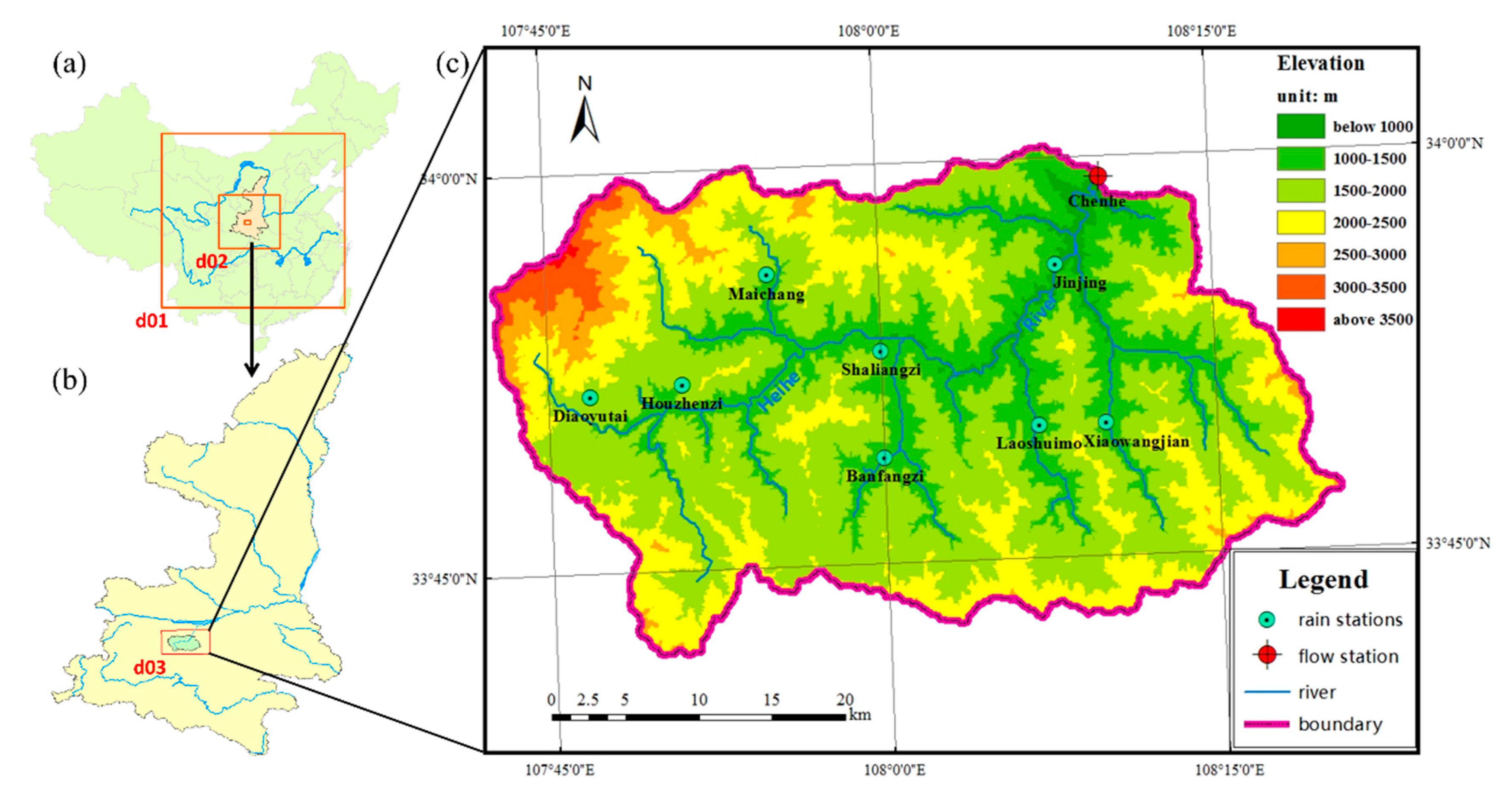
The study area is the Chenhe catchment of 1380 km² in the Yellow River Basin, located in the middle-south Shaanxi Province (Figure 1). The main river of this catchment is called as Heihe River with length of about 105 km. This catchment locates on the northern slope of the Qinling Mountains as one of the main mountain ranges in central China, which is a typical semi-humid catchment with annual mean rainfall of 700–900 mm. The mean elevation of the catchment is about 1819 m a.s.l, with the lowest point at the catchment outlet (579 m a.s.l), and the highest at the Mountain Taibai as the main peak of Qinling Mountains (3771 m a.s.l), and almost 97.7% (1349 km²) of the region above 1000 m. The mean slope is about 26.7°, where the slopes of 86.4% (1193 km²) of the area vary between 10° and 50° and those of 61.9% (854 km²) of area between 20° and 40°.

The Chenhe catchment has a typical temperate continental monsoon climate with mean annual temperature of 12.1 °C, ranging from −1.2 °C in January to 26.5 °C in July. This catchment is prone to frequent severe floods especially during summer and autumn seasons (i.e., flood season, from June 1 to October 31). Rainstorms with high intensity and short duration occur in summer and low intensity and long duration in autumn. According to the USGS 24-category Land Use Categories, vegetation types of the catchment include Savanna (60.9%), Grassland (12.3%), Mixed Forest (8.9%) and Deciduous Broadleaf Forest (7.9%), interspersed with other types (e.g., Shrubland, Cropland, Woodland and Pasture). The surface soil is loamy based on the USGS soil classifications of 16 categories.

The Chenhe gauging station located at the catchment outlet provides rainfall and discharge data. The other eight gauging stations only provide rainfall data. Observations collected from the gauging stations during the flood seasons between 2003 and 2011 are used to produce hourly rainfall and streamflow records using linear interpolation. We adopted 19 typical flood events in this study, and their properties (e.g., duration) are shown in

Table 1. The set of flood events and spin-up period (UTC).

Year	Spin-Up Period	ID	Events	Start	End
2003	1 June 2003, 0:00– 27 August, 18:00	1	030827	27 August, 18:00	4 September, 0:00
		2	030902	2 September, 18:00	9 September, 12:00
		3	030916	16 September, 6:00	24 September, 0:00
2004	1 June 2004, 0:00– 1 September, 6:00	4	040901	1 September, 6:00	9 September, 0:00
2005	1 June 2005, 0:00– 29 June, 18:00	5	050629	29 June, 18:00	4 July, 12:00
		6	050716	16 July, 18:00	19 July, 18:00
2006	1 June 2006, 0:00– 2 September, 18:00	7	060902	2 September, 18:00	7 September, 18:00
		8	060925	25 September, 12:00	3 October, 0:00
2007	1 June 2007, 0:00– 3 July, 18:00	9	070703	3 July, 18:00	7 July, 18:00
		10	070808	8 August, 6:00	13 August, 0:00
2008	1 June 2008, 0:00– 20 July, 6:00	11	080720	20 July, 6:00	23 July, 12:00
2009	1 June 2009, 0:00– 17 August 18:00	12	090817	17 August, 18:00	24 August, 0:00
		13	090910	10 September, 18:00	16 September, 18:00
2010	1 June 2010, 0:00– 21 July, 18:00	14	100721	21 July, 18:00	29 July, 6:00
		15	100820	20 August, 12:00	23 August, 0:00
		16	100822	22 August, 18:00	26 August, 18:00
2011	1 June 2011, 0:00– 3 August, 18:00	17	110803	3 August, 18:00	7 August, 18:00
		18	110909	9 September, 0:00	15 September, 0:00
		19	110916	16 September, 0:00	21 September, 0:00

. The spin-up period of the WRF-Hydro model is set from 1 June to the beginning of the first flood event each year, where its minimum duration is around 30 days in 2005 and the maximum is around 95 days in 2006. Note that the initial condition of the WRF-Hydro model in the spin-up period is identical to that of the WRF model driven by the Final operational global analysis global analysis (FNL) data with the resolution of 0.1°, 6-h, prepared by the National Center for Environmental Prediction (NCEP) (https://rda.ucar.edu/).

2.2. GLDAS

The GLDAS (version 2.1), as a near real-time global terrestrial modeling system incorporating ground observations and satellite data, provides meteorological forcing data on the global scale [29,46] (https://hydro1.gesdisc.eosdis.nasa.gov/data/GLDAS). This product can be used to drive LSMs (e.g., Noah LSM) for simulating evaporation in many regions of China [47,48,49,50]. However, its resolution is too coarse for hydrological simulation of the Chenhe catchment, which is only covered by 3 × 2 GLDAS grids. Therefore, the linear and Bilinear Interpolation Method [51] were employed to disaggregate the 3 h, 0.25° × 0.25° GLDAS product into 1h and 1 km× 1 km resolution. More details about GLDAS are given in [29] and [52].

2.3. The WRF Model

The WRF model, a new generation of mesoscale NWP model, has been widely used in the past 20 years [36,53]. It can produce high-resolution (1–10 km) simulations of meteorological variables such as rainfall [33,34]. The WRF model (version 3.3) was used to generate all forcings for the WRF-Hydro model over study catchment covered by three-nested domains of 25, 5 and 1 km resolution. The outer domain (100 × 95 grids) covers the most of China (22.9°–43.8° N, 95.3°–122.4° E), the middle domain (168 × 146 grids) covers the central China (30.6°–37.1° N, 103.9°–112.8° E) and the inner domain (86 × 51 grids) covers the Chenhe catchment (33.6°–34.1° N, 107.6°–108.5° E) (Figure 1). Time steps are 150, 30 and 6 s for three domains, respectively. Main physical parameterizations of the WRF model are shown in

Table 2. Physical parameterizations of the WRF Model.

Category	Parameterization Selected	References
Microphysical processes	WGM 3-class simple ice model	[54]
Cumulus option	Kain-Fritsch scheme	[55]
Planetary boundary layer	Yonsei University scheme	[56]
Radiation scheme	RRTM, Dudhia	[57]
Land surface model	Noah LSM	[47]
Projection	Lambert	[58]

. The WRF model was driven by the FNL data for each event. Ancillary data, e.g., 30″ land use and soil type, for the inner domain are provided by the static data of WRF Preprocessing System (WPS) (https://www2.mmm.ucar.edu/wrf/users/download).

2.4. The WRF-Hydro Model

2.4.1. A Brief Description

The WRF-Hydro model is a distributed, physical-based and multi-parameterization model with the combined infiltration-excess and saturated-excess runoff module. This model adopts high-resolution routing modules (i.e., overland routing, interflow routing, base-flow routing, channel routing and reservoir or lake routing) to allow multi-scale grids (i.e., LSM grids of kilometers and routing grids of hundreds of meters). Some state variables need to be transmitted between LSM and routing grids when the model is running. For example, soil moisture is mapped from LSM grids onto routing grids. After routing calculation on the fine-resolution grids, the redistribution of soil moisture is aggregated onto LSM grids. The disaggregation-aggregation methodology is described in [23].

Canopy interception of rainfall is described by the water balance equation, and water permeation in subsurface layers is calculated using the Richards Equation [17,48]. Lateral subsurface flow calculated by quasi three-dimensional flow is a function of topography, saturated soil depth and saturated hydraulic conductivity [17,48]. The ponded water comes from three sources: infiltration excess, exfiltration from saturated soil layer and water exchange between grids. Once the ponded water depth exceeds the retention depth, the excess flows freely as surface runoff according to the Shallow Water Wave Equations [59]. A conceptual water bucket model is used to calculate the water storage change under subsurface layers. The Diffusion Wave Equations are used to describe channel routing, where the shape and roughness of each stream order are predefined but can be calibrated. The Manning’s Equation is used in both Shallow Water Wave Equations and Diffusion Wave Equations to simulate friction action on the land surface and channel. More details are available in [17].

2.4.2. Data and Model Settings

The coarse digital elevation and other ancillary data (e.g., land use and soil type) on LSM grids are from the WPS, while high-resolution terrain data required on routing grids are provided by Geospatial Data Cloud site, Computer Network Information Center, Chinese Academy of Sciences (http://www.gscloud.cn/). Other high-resolution fields on routing grids such as flow direction and channel network were obtained through ArcGIS. Note that the channel network was extracted from the fine-scale terrain data with stream definition threshold of 320, thereby yielding a stream below every 20 km² of contributing area in accordance with the actual channel network. The spatial resolutions of the LSM and routing grids are 1 km and 250 m, respectively. The time steps of the terrain and channel routing simulations are 15 s [17]. Main physical parameterizations of the model in this study are shown in

Table 3. The parameterizations of uncoupled WRF-Hydro model.

Category	Parameterization Selected	References
NWP model	WRF model	[36]
Land surface model	Noah LSM	[48]
Subsurface flow (i.e., Interflow)	Distributed hydrology soil and vegetation model	[12]
Overland flow	D8 method	[60]
Baseflow	Exponential storage-discharge function	[17]
Channel routing	Diffusive wave	[59]

.

2.4.3. Calibration of Uncoupled WRF-Hydro Model

The calibration of the uncoupled WRF-Hydro model (version 5.0.3) was only performed in the flood seasons of the first four years (2003–2006) due to high computational cost. For model calibration, the model was only driven by one scenario: GLDAS forcings with observed areal precipitation. Namely, the observed areal precipitation was obtained using the Inverse Distance Weight (IDW) method [61] from rain gauge data, and the other forcings were extracted from the GLDAS product. It is because other spatial interpolation methods (e.g., ordinate kriging method) are not suitable for SMCs due to sparse observation [24], and the GLDAS as a reanalysis product has good performance in evaporation simulation in China [49,50].

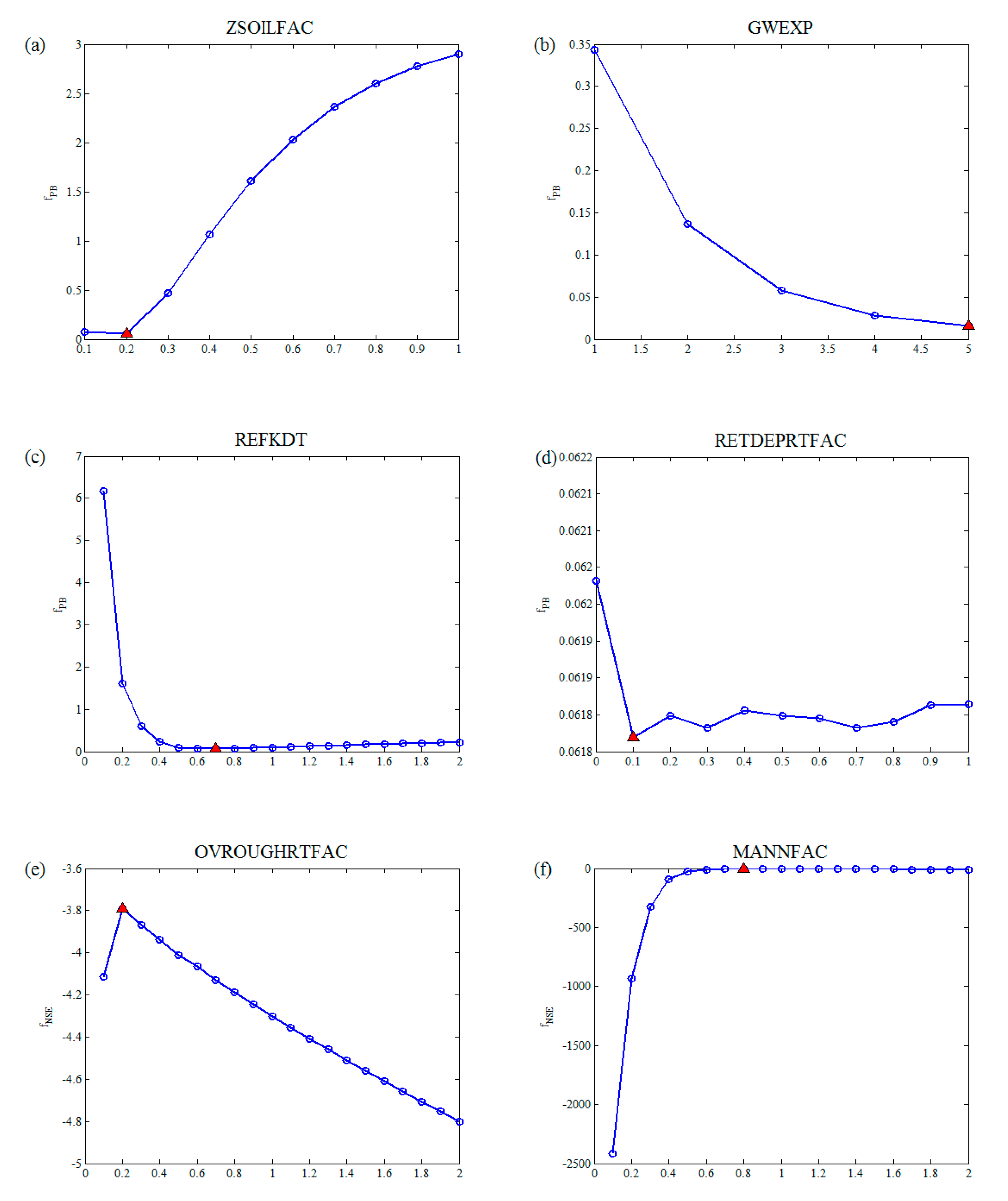
In this study, six model parameters were calibrated including scaling factor on subsurface layer depth (ZSOILFAC), the bucket model exponent of baseflow (GWEXP), referring soil permeability (REFKDT), multiplier on maximum retention depth (RETDEPRTFAC), multiplier on Manning’s roughness for overland flow (OVROUGHRTFAC) and multiplier on Manning’s roughness for channel (MANNFAC). In fact, the soil moisture in the model depends mainly on the subsurface depth, while the predefined depths may be not suitable for the SMCs. The ZSOILFAC is introduced to facilitate the use of variable depths of the four subsurface layers at same scale rather than fixed as 0.05, 0.20, 0.45 and 0.80 m in [25], thereby influencing soil moisture. The specific meaning and function of these six parameters are shown in

Table 4. The parameterizations of WRF-Hydro model.

Name	Meaning	Relevant Variables
ZSOILFAC	Scaling factor on subsurface layer depth	Soil moisture
GWEXP	The bucket model exponent of baseflow	Drainage of groundwater
REFKDT	Referring soil permeability	Infiltration and permeation rates
RETDEPRTFAC	Multiplier on maximum retention depth	Retention depth capacity
OVROUGHRTFAC	Multiplier on Manning’s roughness for overland flow	Overland runoff
MANNFAC	Multiplier on Manning’s roughness for channel	Streamflow

.

The calibration of these parameters adopted the Manual Stepwise Approach [24,25] that selects the best parameter value according to objective function. Two kinds of comprehensive objective functions in terms of percent bias (PB) and Nash-Sutcliffe efficiency coefficient (NSE) were adopted in view of the Compromise Programming Method [62] as follow.

$${\min f}_{\mathrm{PB}}={\displaystyle \sum }_{k=1}^n{\mathrm{PB}}_k^{\alpha },$$

(1)

$$\max f_{\mathrm{NSE}}=1-{\displaystyle \sum }_{k=1}^n{\left({1-\mathrm{NSE}}_k\right)}^{\alpha },$$

(2)

where f_PB and f_NSE represent the objective functions for PB and NSE, respectively, α is the balancing factor and its value takes 4 in accordance with [62], n the number of events in calibration period and k the event number. The f_PB is used to gain the optimum values of ZSOILFAC, GWEXP, REFKDT and RETDEPRTFAC since these parameters have an impact on flood volume, and the f_NSE the optimum values of OVROUGHRTFAC and MANNFAC since they influence the hydrograph shape. Figure 2 shows the sensitivity analysis for these six parameters, and the calibration ranges and steps of the parameters are shown in

Table 5. The ranges and increments of main model parameters for the Manual Stepwise Approach.

Parameter	ZSOILFAC	GWEXP	REFKDT	RETDEPRTFAC	OVROUGHRTFAC	MANNFAC
Lower	0.1	1.0	0.1	0.0	0.1	0.1
Upper	1.0	5.0	2.0	1.0	2.0	2.0
Increment	0.1	1.0	0.1	0.1	0.1	0.1

. As a result, the optimum solutions are 0.2, 5.0, 0.7, 0.1, 0.2 and 0.8 for ZSOILFAC, GWEXP, REFKDT, RETDEPRTFAC, OVROUGHRTFAC and MANNFAC, respectively.

2.5. The Xinanjiang Model

The Xinanjiang model [63], a conceptual semi-distributed hydrologic model, is widely used in flood forecasting for humid and semi-humid watersheds in China [64,65,66,67]. It has four major components: runoff generation, evapotranspiration, separation of runoff components and flow concentration with main inputs of the model including observed rainfall and pan evaporation [63,68]. The Major model parameters are shown in

Table 6. The values and their functions of main parameters for the Xinanjiang model.

Parameter	Value	Meaning	Function
K	0.5	The ratio of potential evapotranspiration to pan evaporation	Controlling the simulated water volume
WM	160 mm	Tension water storage capacity
SM	14 mm	Gravity water storage capacity	Controlling the simulated hydrograph shape
CS	0.08	The recession coefficient of runoff in channel network

. Note that the Xinanjiang model was utilized as a tool for investigating the flood prediction capability of the WRF-Hydro model owing to the satisfactory performance and application in Chenhe catchment.

2.6. Forcing Scenarios Design

It is very significant for the WRF-Hydro model to choose the adequate and appropriate forcings at first. Currently, there are three prominent methods to obtain the forcing data. Firstly, all forcings derive from one source directly such as the WRF outputs and the Global Forecast System [24,28,69,70,71]. Secondly, forcings are from the combination of several products [19,25,72]. For example, reference [25] acquired rainfall, air temperature, air pressure and air humidity from observation, wind speed and incoming shortwave radiation from merged products, and incoming shortwave radiation from the GLDAS. Lastly, forcings are provided by the WRF model using the fully coupled WRF-Hydro modeling system [25,26].

In this study, we adopted the second method to generate the forcings of the uncoupled WRF-Hydro model. Eight forcing scenarios (

Table 7. The key information of eight forcing scenarios in this study ¹.

Number	Scenario 2	Model	Input Meteorological Forcings
			Rainfall	The Remaining Forcings
1	G + Gr 3	WRF-Hydro	GLDAS-derived rainfall	GLDAS
2	G + I		IDW product	GLDAS
3	W + Wr 4		WRF-derived rainfall	WRF
4	W + I		IDW product	WRF
5	G + Gm		GLDAS-merged rainfall	GLDAS
6	W + Wm		WRF-merged rainfall	WRF
7	I + I		IDW product	Ideal forcings 5
8	XAJ	Xinanjiang	Rain gauge data and pan evaporation

¹ See Section 2.6; ² The abbreviation of each experiment; ³ All forcings in this scenario derive from the GLDAS product; ⁴ All forcings in this scenario derive from the WRF outputs; ⁵ It can be generated by the WRF-Hydro model when there are not any forcings available in a catchment, and more detail in Table 8.

) were designed to find out the appropriate forcings and to assess the performance of the WRF-Hydro model in SMCs. In fact, the forcings required in this model are classified as rainfall and the remaining forcings. Rainfall products in this study include IDW product, GLDAS-derived rainfall (Gr), WRF-derived rainfall (Wr), GLDAS-merged rainfall (Gm) and WRF-merged rainfall (Wm). The Successive Corrections Method [42,43,44,45] was adopted as a precipitation merging method, where its weight function takes the Cressman Weight Function [73], the number of iterations 5, and influence radius 100 km. The remaining forcings contain GLDAS, WRF and ideal forcings. The values of ideal forcings [17] generated by the WRF-Hydro model are shown in

Table 8. The values of ideal forcings.

Variable Name	Description	Prescribed Value or Range	Timing
SWDOWN	Incoming shortwave radiation	0–900 W/m2	Diurnal cycle
LWDOWN	Incoming longwave radiation	375–425 W/m2	Diurnal cycle
Q2D	specific humidity	0.01 kg/kg	Constant
T2D	Air temperature	287–293 K	Diurnal cycle
PSFC	Surface pressure	100,000 Pa	Constant
U2D	Near-surface wind speed in the u-component	1.0 m/s	Constant
V2D	Near-surface wind speed in the v-component	1.0 m/s	Constant

.

2.7. Evaluation Metrics

The accuracy of the rainfall, evapotranspiration (ET) and streamflow are characterized by five assessment metrics: percent bias (PB), root mean square error (RMSE), correlation coefficient (RR), Nash-Sutcliffe efficiency coefficient (NSE) and Shannon entropy (SE).

$$\mathrm{PB}=\frac{{\displaystyle {\displaystyle \sum }_{i=1}^n}\left(s_i{-o}_i\right)}{{\displaystyle {\displaystyle \sum }_{i=1}^n}{o}_i},$$

(3)

$$\mathrm{RMSE}=\sqrt{\frac{1}{n}{\displaystyle \sum }_{i=1}^n{\left(s_i{-o}_i\right)}^2},$$

(4)

$$\mathrm{RR}=\frac{{\displaystyle {\displaystyle \sum }_{i=1}^n}\left(s_i-\overline{s}\right)\left(o_i-\overline{o}\right)}{\sqrt{{\displaystyle {\displaystyle \sum }_{i=1}^n}{\left(s_i-\overline{s}\right)}^2}\sqrt{{\displaystyle {\displaystyle \sum }_{i=1}^n}{(o_i-\overline{o})}^2}},$$

(5)

$$\mathrm{NSE}=1-\frac{{\displaystyle {\displaystyle \sum }_{i=1}^n}{\left(s_i{-o}_i\right)}^2}{{\displaystyle {\displaystyle \sum }_{i=1}^n}{(o_i-\overline{o})}^2},$$

(6)

$$\mathrm{SE}(\overrightarrow{x})=-{\displaystyle \sum }_{k=1}^{N}p(x_k){\log }_2(p(x_k)) \overrightarrow{x}={(x_1,x_2,\cdots ,x_N)}^T,$$

(7)

where s_i is the simulated results for each time step i, o_i is the observed value, n is the total number of time series, $\overrightarrow{x}$ is a discrete random variable recording all different values in the grids, p(x_k) is the frequency of value of x_k appearing in the grids and N is the length of the $\overrightarrow{x}$. The PB and RMSE measure the errors of simulated results, and the RR and NSE quantify the degree-of-fit between simulation and observation. The SE is regarded as a measure for spatial variability and the higher its values are, the more complex related spatial information is. Note that the SE is only calculated within the Chenhe catchment according to the spatially distributed rainfall or ET with 0.1 mm accuracy.

3. Results and Discussion

To evaluate the quality of precipitation, we first compared the five rainfall products (i.e., IDW, Gr, Wr, Gm and Wm) using the metrics PB, RMSE and SE. Then, the WRF-Hydro-derived simulated ET of the three scenarios (i.e., G + I, W + I and I + I) was analyzed through the PB, RMSE, RR and SE to understand the impact of different forcings (without rainfall). Finally, we compared simulated streamflow of the eight scenarios (i.e., G + Gr, G + I, W + Wr, W + I, G + Gm, W + Wm and I + I and XAJ) at the outlet via the same metrics.

3.1. Evaluation of Five Rainfall Products

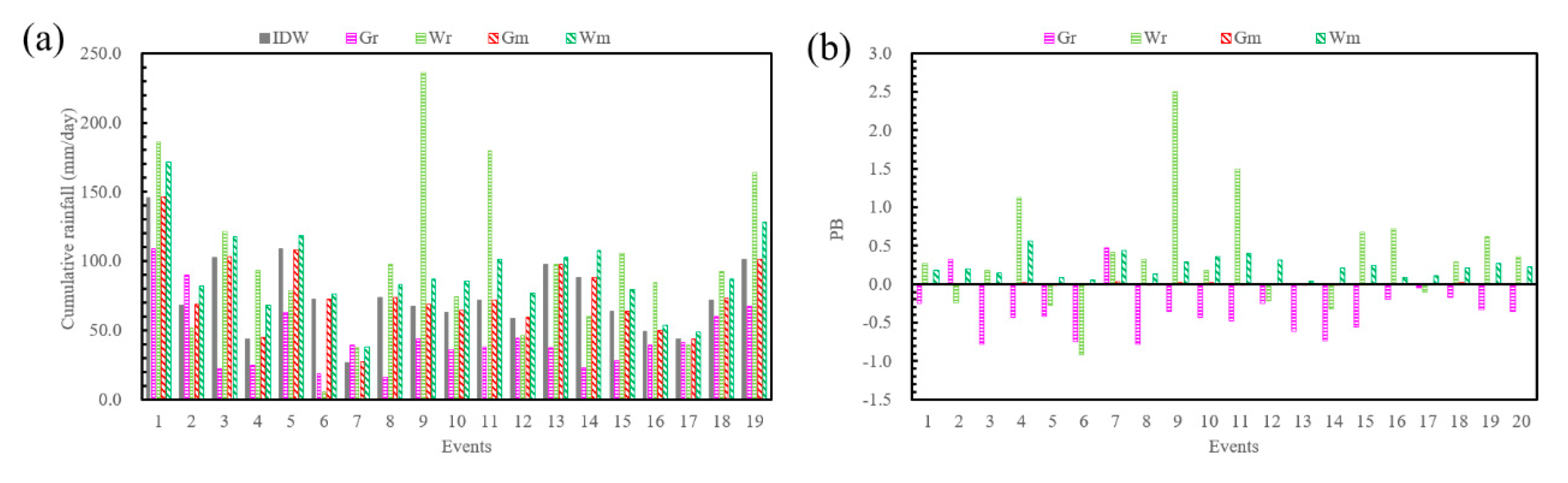
As mentioned above, we regarded the IDW product as observed areal precipitation. The cumulative rainfall of the IDW, Gr, Wr, Gm and Wm is shown in Figure 3a, and the PB of the last four products in Figure 3b. The Gr and Wr show relatively poor performance in terms of the PB (Figure 3b). Significant negative errors are observed in 89.5% of events of the Gr, with mean rainfall only 44.4 mm approximately 60% of the observed rainfall (74.7 mm). This is arguably due to information loss in the coarse-scale grids. While an overestimation of rainfall is found in the Wr for 68.4% of events, with mean rainfall up to 97.5 mm nearly 1.3 times higher than the observation counterpart. However, the results of the PB in the Gm and Wm are improved when the Successive Corrections Method was applied (Figure 3b). The PB mean-values of the Gm and Wm have dropped from −0.357 in Gr to 0.007 and from 0.353 in Wr to 0.228, respectively.

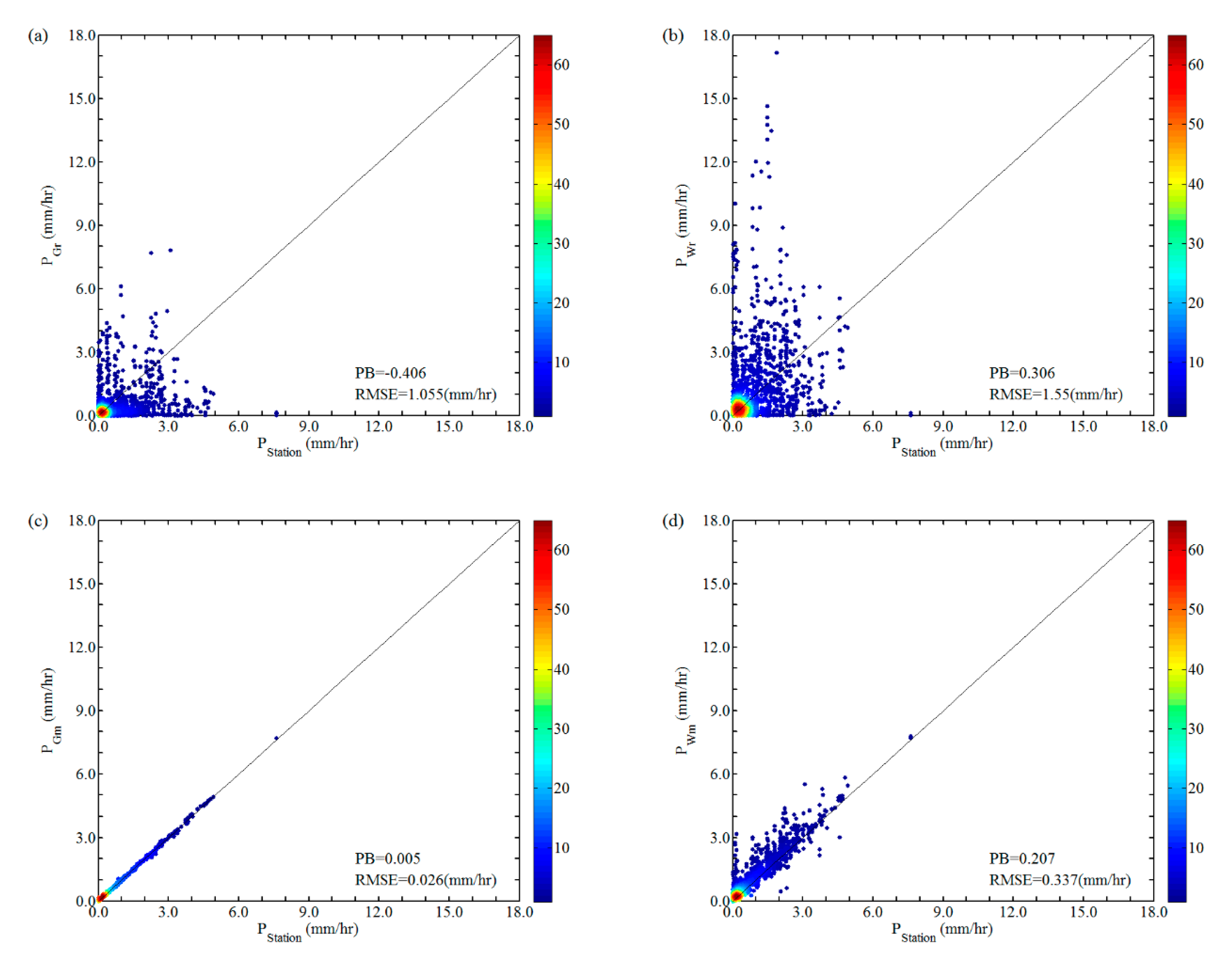
We further compared the hourly-scale rainfall series of four products before and after merging with observation for all events (Figure 4). As shown in Figure 4a,b, the Gr has large negative bias (PB = −0.406), while the Wr has positive bias (PB = 0.306) compared to observation. The Wr has higher RMSE (1.550 mm/h) than the Gr (1.055 mm/h), confirming that raw rainfall of the WRF model overestimates the hourly areal mean rainfall [36], even though the Wr has finer spatial resolution. Once merging with gauging data, the Gr improves with RMSE-value soaring from 1.055 to 0.026 mm/h, and the Wr also has a satisfying performance with RMSE-value increasing from 1.550 to 0.337 mm/h. Compared with raw products, the quality of rainfall from the GLDAS and WRF is improved through the merging. The Gm performs better than the Wm possibly resulting from the coarser spatial resolution.

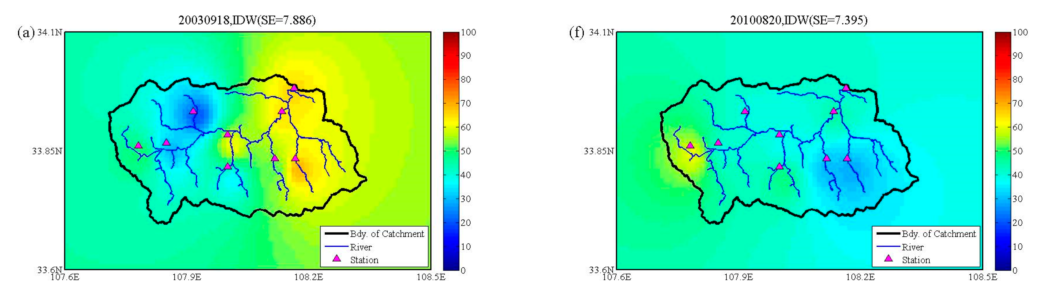
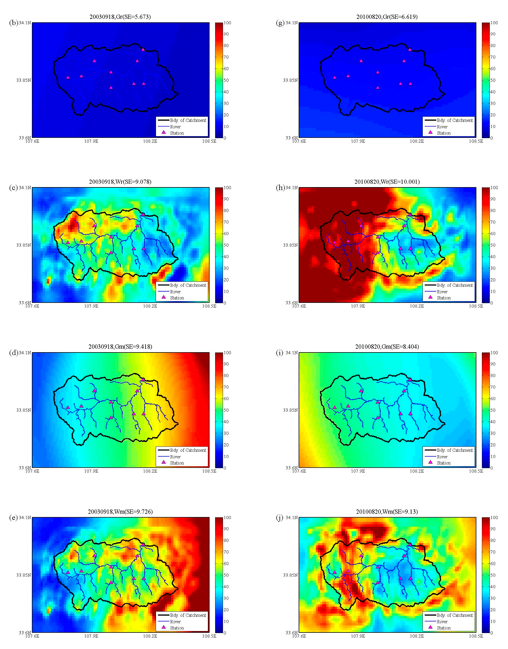
After comparing the rainfall and time series, we investigated the spatial distributions of cumulative rainfall on the highest rainfall day, e.g., September 18 for event 030916 and August 20 for event 100820 (Figure 5). The IDW product is able to capture the general features of rain distribution (e.g., storm center), while its quality normally depends on the density and location of rain gages. The Gr has a smooth spatial distribution nearly without any peaks or depressions and with lower SE-values compared to others (5.67 and 6.62 for event 030916 and 100820, respectively), while the Wr has higher values of SE (9.08 and 10.00 for event 030916 and 100820, respectively). After merging with observation, the volume and spatial variability of rainfall products have been improved (Figure 5b–e,g–j), owing to assimilation of field observations. As a result, the quality and reliability of the Gm and Wm outperform those of Gr and Wr to flood simulation of the WRF-Hydro model in terms of the spatial distributions.

To further illustrate the impact of merging method on the spatial distributions of the rainfall products, we also calculated the PB and RMSE of Gr, Gm, Wr and Wm based on the cumulative rainfall on the highest rainfall day at 9 rain gauges for all events (Figure 6). The PB-distributions of the Gm and Wm narrow around 0-line, and the majority of RMSE-values decline from above 50 mm (68.4% and 63.2% for the Gr and Wr, respectively) to below 50 mm (84.2% and 68.4% for the Gm and Wm, respectively). Therefore, the accuracy and spatial variability have been improved after merging with observations, at least for 9 stations. Consequently, the IDW, Gm and Wm are more suitable than the others for hydrological simulation of the WRF-Hydro model.

3.2. Evaluation of Daily WRF-Hydro-Derived ET in Three Scenarios

Except rainfall, the remaining forcings also have an effect on the streamflow simulation of the WRF-Hydro model, and they are mainly utilized to calculate potential evaporation through Penman-Monteith Equation, thereby affecting the simulated ET in the model. Therefore, the difference of the forcings (without rainfall) can be indirectly quantified through the ET comparison. To make the results comparable, we analyzed the daily ET of three scenarios, G + I, W + I and I + I, using pan evaporation data collected at Heiyukou (HYK) Station. Note that the pan evaporation only provides a reference for evaluating simulation since it only represents the one-point water surface evaporation rather than actual ET. The hourly cumulative simulated ET from the model was transformed into daily ET to keep consistent with the observation.

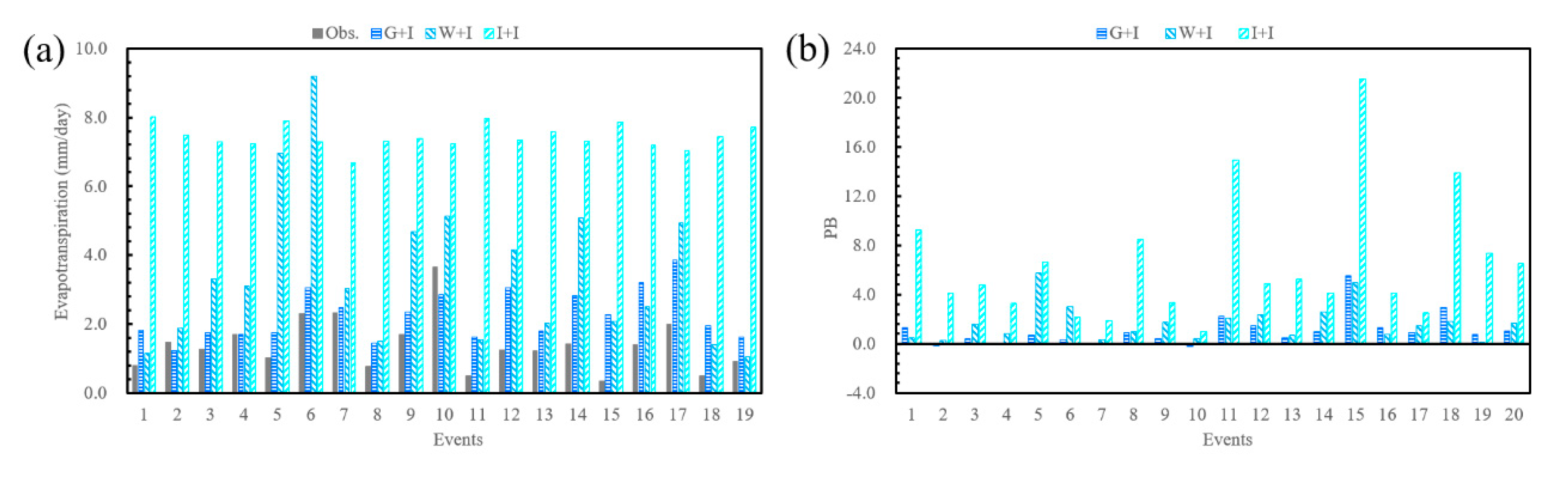
Figure 7a shows the daily mean ET-volume of observation, G + I, W + I and I + I, and Figure 7b corresponding PB of the three scenarios at the grid containing HYK station for each event. The simulated ET of G + I has a smaller PB mean-value (1.063) than those of other scenarios, confirming that the GLDAS-derived forcings (without rainfall) have good skill in simulating ET despite relatively coarse spatial distribution of GLDAS products (3 h, 0.25°). The simulated ET of W + I has intermediate performance with mean PB of 1.690, indicating it is suitable for study catchment to use the high-resolution forcings (without rainfall) of WRF model (1 h, 1 km) to calculate ET, especially when the catchment area is small covered by a few GLDAS grids. The simulation of scenario I + I performs poorly compared to the others in terms of the PB (6.497), which overestimates ET clearly. It is attributed to the oversimplified generalization scheme of ideal forcings (Table 8). It implies that the forcings (without rainfall) from the GLDAS and the WRF are recognized as the suitable ones according to the PB of the ET volume when the rainfall is identical.

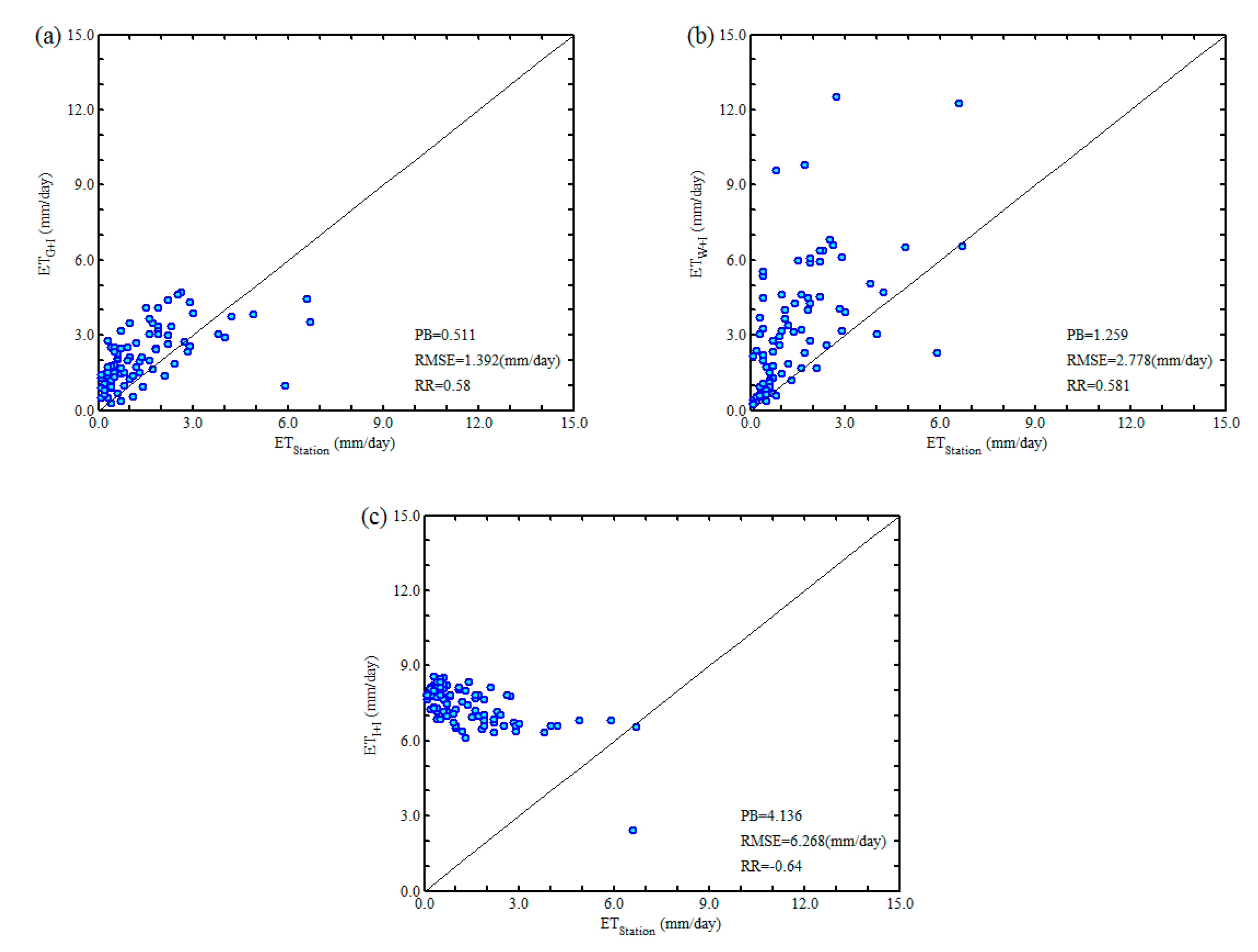
We further compared daily-scale simulated ET series of the three scenarios with pan evaporation at HYK Station, respectively (Figure 8). The daily ET of the G + I has a better performance than the others with narrower spread and smaller bias in terms of PB, RMSE and RR (Figure 8). Scenario W + I performs moderately, and most points (89.2% versus 81.9% in G + I) are above the 45° line. The PB of the W + I (1.259) is twice greater than that of the G + I (0.511), and RR of the W + I (0.581) is close to that of the G + I (0.580). The ET from scenario I + I is overestimated for nearly all points (98.8%) despite its narrower distribution (range: 2.4 mm/day). The overestimations of ET at the grid containing HYK station are observed in the three scenarios, possibly because the potential evaporation is overestimated at this grid when the model is driven by these forcings (without rainfall). Compared with scenario W + I and I + I, scenario G + I produces the best simulated ET, and GLDAS-derived forcings (without rainfall) can serve as good ones to the WRF-Hydro model for the study catchment.

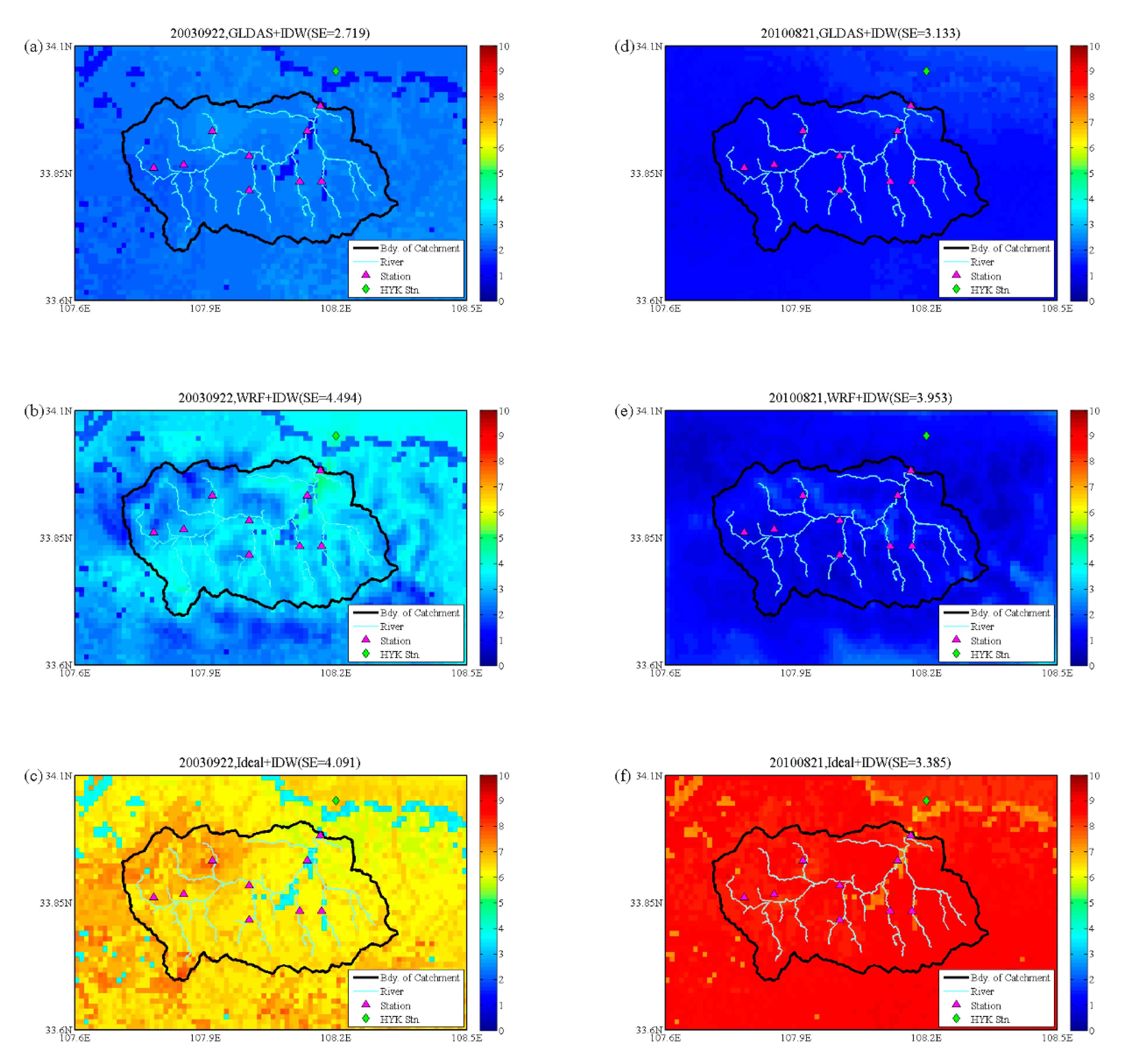
In order to learn the spatial pattern of simulated ET in the three scenarios, we took events 030916 and 100820 on the highest observed ET day (i.e., September 22 for event 030916 and Auguat 21 for event 100820) for example. As shown in Figure 9, the spatial distribution of ET in scenario W + I unanimously has the highest SE (4.494 in 030916 and 3.953 in 100820), suggesting that the forcings (without rainfall) of the WRF model outputs capture the ET distribution. The G + I simulations have lowest SE (2.719 in 030916 and 3.133 in 100820) compared to the others, arguably due to the coarse resolution of the GLDAS data. The ET is overestimated over the whole catchment when using scenario I + I to drive the WRF-Hydro model even if this scenario yields moderate SE (4.091 in 030916 and 3.385 in 100820). This implies that the overestimation of ET for the I + I may occur not only at Heiyukou station, but also catchment-wide due to the generation pattern of the ideal forcings (Table 8). Consequently, the forcings (without rainfall) derived from the GLDAS and WRF show good skills in ET simulation according to error, correlation and spatial variability and are identified as good data set for the hydrological simulation of the WRF-Hydro model in the Chenhe catchment.

3.3. Evaluation of Streamflow for the Eight Scenarios

We first compared the streamflow simulations of the WRF-Hydro model among the seven forcing scenarios (G + Gr, G + I, W + Wr, W + I, G + Gm, W + Wm and I + I) (Figure 10 and

Table 9. The mean values of four metrics shown in Figure 10.

	G + Gr	G + I	W + Wr	W + I	G + Gm	W + Wm	I + I	XAJ
PB	−0.510	0.063	0.752	0.009	0.063	0.331	−0.291	0.147
RMSE (mm/h)	0.41	0.18	0.74	0.18	0.17	0.23	0.23	0.17
RR	0.031	0.852	0.533	0.837	0.844	0.899	0.770	0.934
NSE	-0.47	0.61	−15.36	0.61	0.61	0.46	0.37	0.71

), and then compared the three best results of the WRF-Hydro model (i.e., scenarios G + I, W + I and G + Gm) with the result of the Xinanjiang model (i.e., scenario XAJ) (Figure 11 and Figure 12). Note that the calibration of the WRF-Hydro model was only preformed in scenario G + I, and the parameters after calibration were adopted in the other scenarios.

3.3.1. Comparison of the Scenarios Using the WRF-Hydro Model

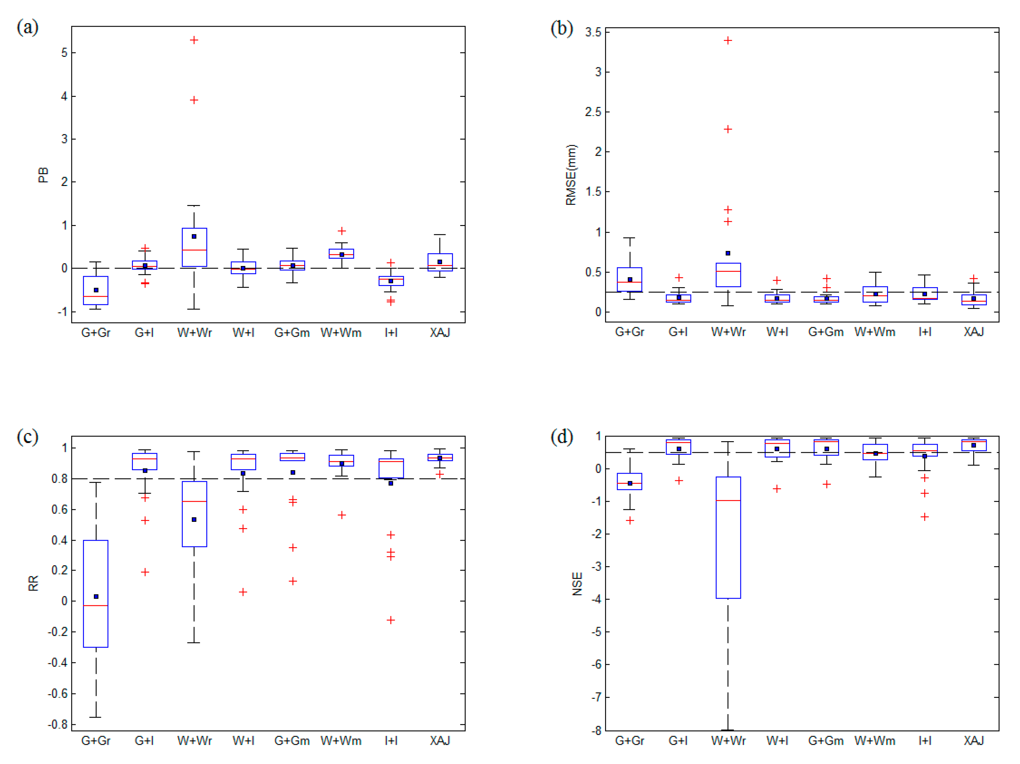
Scenarios G + I, W + I and G + Gm perform well, indicated by smaller PB (0.009–0.063) and RMSE (<0.2 mm/h) and narrower spreads than other scenarios using the WRF-Hydro model, similar to that of scenario XAJ (Figure 10). These results indicate that scenarios G + I, W + I and G + Gm have good and similar performances when regarding them as forcings to drive the WRF-Hydro model.

To analyze how different forcings (without rainfall) influence the streamflow pattern, we also compared scenarios G + I, W + I and I + I (Figure 10). For scenario I + I, the RR and NSE are moderate, while the 84.2% of PB-values are below 0 and the RMSE-spread is wider than corresponding values of the G + I and W + I (Figure 10c,d). The underestimation of streamflow of scenario I + I (PB = −0.291) is largely due to the overestimation of ET (PB = 6.497), further revealing that different forcings (without rainfall) have a non-ignorable impact on streamflow reproduction.

We further compared scenarios G + Gr, W + Wr, G + Gm and W + Wm to understand the impact of merged rainfall on the discharge simulation (Figure 10). Scenario G + Gr exhibits poor performance with higher PB and RMSE (Table 9), implying that the underestimation of Gr (PB = −0.357) is likely to be responsible for the discharge underestimation. Scenario W + Wr also yields a poor result and overestimates streamflow possibly due to large positive error of Wr (PB = 0.353). However, not only the flood volume but also correlation and shape of hydrograph are improved when Gr is replaced by Gm and Wr by Wm (Figure 10b,d). The mean RMSEs of scenarios G + Gm and W + Wm are as low as 0.17 and 0.23 mm/h, respectively, while 0.41 and 0.74 mm/h for the G + Gr and W + Wr, respectively. As a result, the merged rainfall lead to improved streamflow simulation with the mean RMSEs improved by 58.5% and 68.9% for G + Gm and W + Wm, respectively.

Many noticeable outliers (i.e., the points outside of the 5th to 95th percentiles in box plots) are observed for three primary reasons (Figure 10). Firstly, the whole distributions are excellent, and thus some acceptable values are recognized as outliers such as the G + Gm (Figure 10b). Secondly, large positive bias in WRF-derived rainfall causes outliers such as the W + Wr (Figure 10c). Thirdly, the overestimation of ET in scenario I + I leads to negative bias in streamflow reproduction such as the I + I (Figure 10d). Moreover, events with smaller peak flow (e.g., Event 040,901 with peak flow of 153 m³/s) always exhibit poor performance regardless of forcings, possibly because the duration of spin-up period is too short to obtain suitable initial state.

It is emphasized that the local observation at rain gauges and global, spatially-distributed GLDAS product and FNL data driving the WRF model are available in general SMCs or regions. To study the feature of these data is significant for the hydrometeorological simulation using the WRF-Hydro model to SMCs, especially for the regions with sparse observation. Scenarios G + I, G + Gm and W + I are likely to yield good performances for other SMCs lacking observed forcings. Scenario W + Wm may be more suitable for these catchments when the WRF model uses appropriate parameterization with high-quality input or when data assimilation technologies are used in WRF model.

3.3.2. Comparison of the WRF-Hydro and Xinanjiang Model

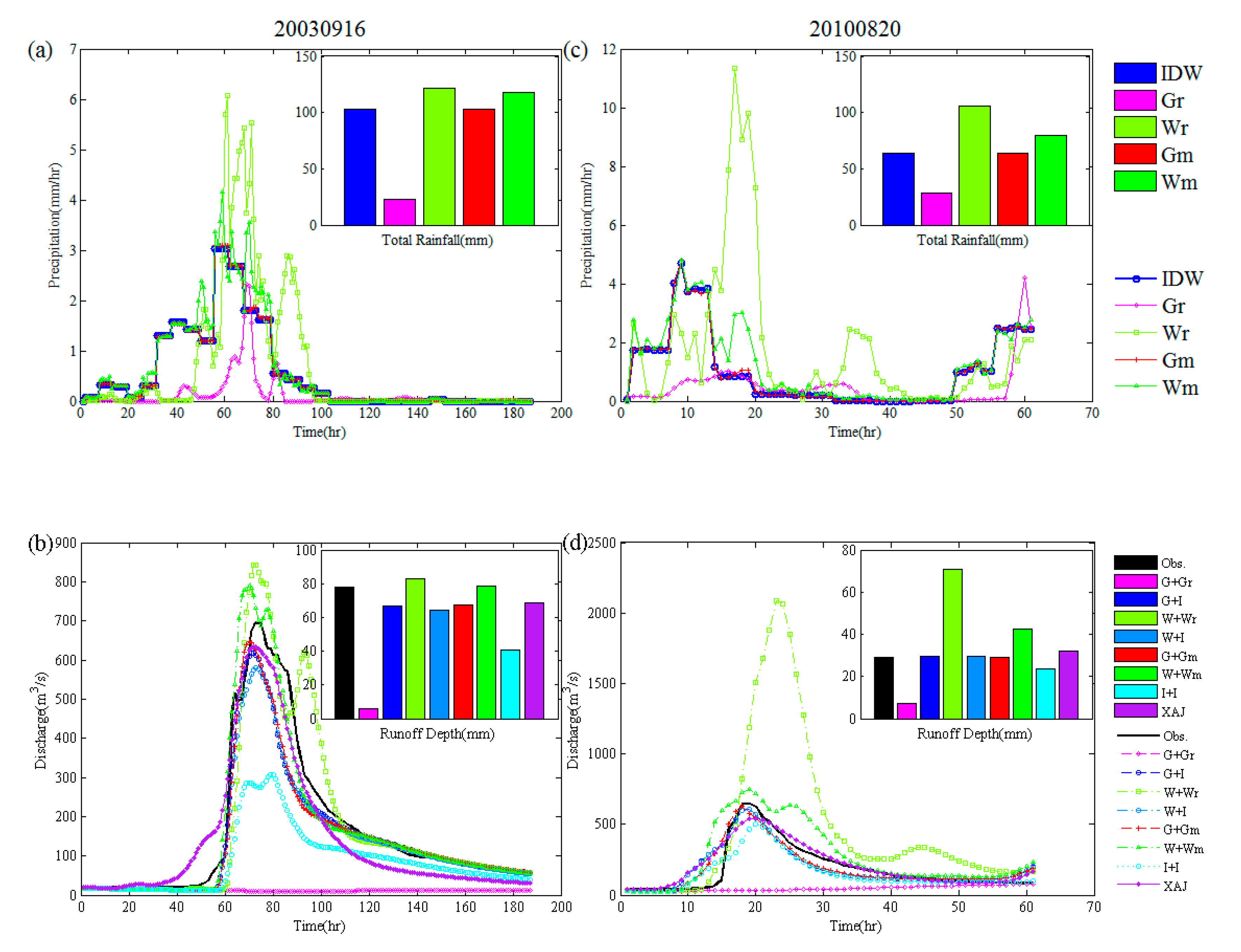
To evaluate the flood prediction capability of the WRF-Hydro model, we only compared the best results of the model (i.e., scenarios G + I, W + I and G + Gm) with the result of the Xinanjiang model (i.e., scenario XAJ). As shown in Figure 10a, the results in scenarios G + I, W + I and G + Gm have a narrower spread than scenario XAJ in terms of the PB and RMSE (Table 9). The RR and NSE of scenario XAJ are better than those of scenarios G + I, W + I and G + Gm (Table 9). It indicates that the WRF-Hydro model has good skills to simulate the flood volume, while the Xinanjiang model performs well in describing the flood hydrograph. Figure 11 shows the rainfall, runoff depth and hydrographs of the two events, 20030916 and 20100820. After merging with observations, the total areal mean rainfall of Gm is consistent with that of IDW product for the two cases (Figure 11a,b). The underestimation of runoff depth is observed in scenarios G + I (PB = −0.141), W + I (PB = −0.176), G + Gm (PB = −0.140) and XAJ (PB = −0.119) for event 20,030916 (Figure 11c,d). The scenarios G + I (PB = 0.019), W + I (PB = 0.020) and G + Gm (PB = 0.014) perform better than scenario XAJ (PB = 0.110) in terms of runoff depth for event 20100820.

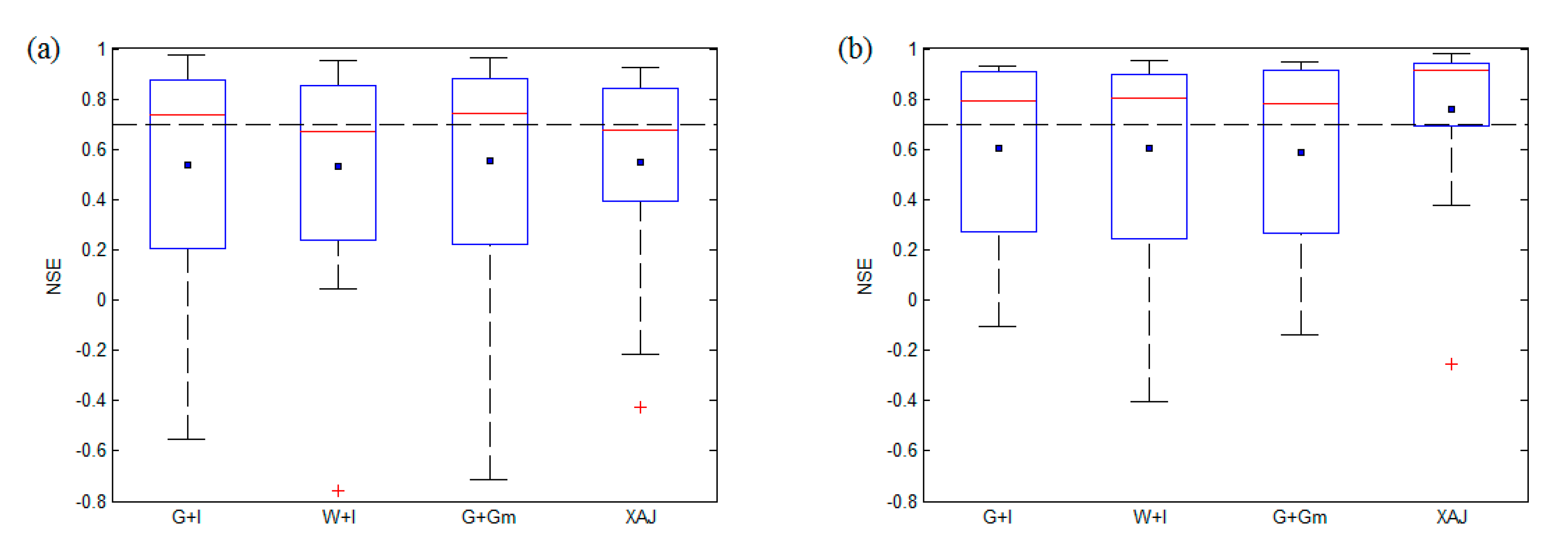
The flood hydrographs of scenarios G + I, G + Gm and W + I indicate that the WRF-Hydro model may be better at describing the rising limb of flood hydrographs. To further investigate this phenomenon, the degree-of-fit of flood hydrograph in rising and falling limbs was calculated through the NSE where the rising limb is from the start to the flood peak time and the rest is falling limb (Figure 12). The WRF-Hydro model has wider NSE-distribution than the Xinanjiang model for rising and falling limbs. The NSE of the rising limb in around half of the events (52.6%, 47.4% and 63.2% for G + I, W + I and G + Gm, respectively) exceed 0.7 versus 47.4% of the Xinanjiang model (Figure 12a). Our analysis confirms that the WRF-Hydro model performs well in simulating rising limb at least in half of the events. Similar NSE-distribution is obtained for the falling limb, but corresponding NSEs are closer to 1.0 for the two models (Figure 12b). The Xinanjiang model with NSE-values in 68.4% of events greater than 0.7 has a narrower spread than that of the WRF-Hydro model. In fact, the low NSEs of the two models often appear in events with small peak flow where the Xinanjiang model outperforms the WRF-Hydro model. As a result, these two models exhibit similar performances for the events with higher NSEs (i.e., NSE ≥ 0.7), while the WRF-Hydro model shows moderate results for the events with lower NSEs (i.e., NSE < 0.7). It is possibly because the simulation of the WRF-Hydro model is more sensitive to the quality of inputs than that of the Xinanjiang model.

The Xinanjiang model was adopted to assess the flood prediction capacity of the WRF-hydro model, and their performance difference is mainly caused by the two points: model structure and input-output data. On the one hand, the conceptual Xinanjiang model adopts the three-layer soil moisture model [63] to calculate the ET, which aims at water balance in hydrological simulation. The saturated-excess runoff module is another characteristic of this model [63]. As a semi-distributed model, it adopts the tension water capacity curve [63] to represent the spatial inhomogeneity of soil moisture. By contrast, the WRF-Hydro model simulates the ET with the Noah or Noah-MP LSM taking account of water and energy balance [48]. This model adopts the combined infiltration-excess and saturated-excess runoff module for runoff calculation. The orthogonal grids are used in the LSM and routing grids to represent the spatial distribution of hydrometeorological variables and parameters. On the other hand, the inputs of the Xinanjiang model only include precipitation and pan evaporation. Its outputs contain ET, the discharge at the outlet of the watershed and the areal mean soil moisture. It is not easy for the Xinanjiang model to absorb some useful meteorological data (e.g., radiation and wind speed) and to obtain the distributed simulation. However, the WRF-Hydro model requires substantial spatial inputs including the forcings, underlying surface state and corresponding parameters and produces spatial outputs including distributed streamflow, water and energy flux and hydrometeorological states. This model assimilates lots of effective information to achieve spatial hydrological simulation, although this simulation is sensitive to the quality of inputs. In addition, it is easy to fully couple with the WRF model for the operational hydrometeorological prediction. Therefore, the WRF-Hydro model has promising potential for flood forecasting in the Chenhe catchment.

4. Conclusions

Based on the observed and merged rainfalls, GLDAS, WRF outputs and ideal forcings, seven scenarios were designed (G + Gr, G + I, W + Wr, W + I, G + Gm, W + Wm and I + I) for driving the WRF-Hydro model to simulate floods of the Chenhe catchment. It is indicated that the WRF-Hydro model can yield better results when driven by the scenarios G + I, W + I or G + Gm than other scenarios using the WRF-Hydro model (i.e., G + Gr, W + Wr, W + Wm and I + I).

It is not recommended to use directly the GLDAS- and WRF-derived rainfalls to simulate the floods of the Chenhe catchment. The flood simulations can be improved when using GLDAS- and WRF-merged rainfalls. The WRF-Hydro model tends to overestimate the ET and subsequently to underestimate the streamflow when using the ideal forcings (without rainfall). However, the model produces better ET simulations when using the forcings (without rainfall) from the GLDAS and WRF.

Although the performance of the WRF-Hydro and Xinanjiang models is generally comparable, the WRF-Hydro model can produce spatially distributed outputs such as evaporation, streamflow and soil moisture. The WRF-Hydro model shows promising potential for operational flood forecasting of the Chenhe catchment, and we plan to conduct more studies on the application of the WRF-Hydro model to other SMCs with different hydroclimatic patterns to further explore its suitability. Additionally, this model has the potential to extend the lead time of operational flood forecasting since it can be fully coupled with the WRF model. This study facilitates the application of the WRF-Hydro model in worldwide SMCs for hydrometeorological simulation, especially for the SMCs with sparse observation.

References

- Jonkman, S.N. Global Perspectives on Loss of Human Life Caused by Floods. Nat. Hazards 2005, 34, 151–175. [Google Scholar] [CrossRef]
- Ronco, P.; Gallina, V.; Torresan, S.; Zabeo, A.; Semenzin, E.; Critto, A.; Marcomini, A. The KULTURisk Regional Risk Assessment methodology for water-related natural hazards—Part 1: Physical–environmental assessment. Hydrol. Earth Syst. Sci. 2014, 18, 5399–5414. [Google Scholar] [CrossRef] [Green Version]
- He, B.S.; Huang, X.L.; Ma, M.H.; Chang, Q.R.; Tu, Y.; Li, Q.; Zhang, K.; Hong, Y. Analysis of flash flood disaster characteristics in China from 2011 to 2015. Nat. Hazards 2018, 90, 407–420. [Google Scholar] [CrossRef]
- Sun, Q.; Hu, J.; Zhang, L.; Ding, X.L. Towards Slow-Moving Landslide Monitoring by Integrating Multi-Sensor InSAR Time Series Datasets: The Zhouqu Case Study, China. Remote Sens. 2016, 8, 908. [Google Scholar] [CrossRef] [Green Version]
- Zhang, K.; Xue, X.W.; Hong, Y.; Gourley, J.J.; Lu, N.; Wan, Z.M.; Hong, Z.; Wooten, R. iCRESTRIGRS: A coupled modeling system for cascading flood-landslide disaster forecasting. Hydrol. Earth Syst. Sci. 2016, 20, 5035–5048. [Google Scholar] [CrossRef] [Green Version]
- Chao, L.J.; Zhang, K.; Li, Z.J.; Wang, J.F.; Yao, C.; Li, Q.L. Applicability assessment of the CASCade Two Dimensional SEDiment (CASC2D-SED) distributed hydrological model for flood forecasting across four typical medium and small watersheds in China(Article). J. Flood Risk Manag. 2019, 12, e12518. [Google Scholar] [CrossRef] [Green Version]
- Liu, Z.; Todini, E. Towards a comprehensive physically-based rainfall-runoff model. Hydrol. Earth Syst. Sci. 2002, 6, 859–881. [Google Scholar] [CrossRef]
- Todini, E. Rainfall-runoff modeling—Past, present and future. J. Hydrol. 1988, 100, 341–352. [Google Scholar] [CrossRef]
- Yao, C.; Li, Z.J.; Yu, Z.B.; Zhang, K. A priori parameter estimates for a distributed, grid-based Xinanjiang model using geographically based information. J. Hydrol. 2012, 468, 47–62. [Google Scholar] [CrossRef]
- Beven, K.; Binley, A. The future of distributed models: Model calibration and uncertainty prediction. Hydrol. Process. 1992, 6, 279–298. [Google Scholar] [CrossRef]
- Rozalis, S.; Morin, E.; Yair, Y.; Price, C. Flash flood prediction using an uncalibrated hydrological model and radar rainfall data in a Mediterranean watershed under changing hydrological conditions. J. Hydrol. 2010, 394, 245–255. [Google Scholar] [CrossRef]
- Wigmosta, M.S.; Lettenmaier, D.P.; Vail, L.W. A distributed hydrology-vegetation model for complex terrain. Water Resour. Res. 1994, 30, 1665–1679. [Google Scholar] [CrossRef]
- Anderson, M.L.; Chen, Z.-Q.; Kavvas, M.L.; Feldman, A. Coupling HEC-HMS with Atmospheric Models for Prediction of Watershed Runoff. J. Hydrol. Eng. 2002, 7, 312–318. [Google Scholar] [CrossRef]
- Yu, Z.B.; Lakhtakia, M.N.; Yarnal, B.; White, R.A.; Miller, D.A.; Frakes, B.; Barron, E.J.; Duffy, C.; Schwartz, F.W. Simulating the river-basin response to atmospheric forcing by linking a mesoscale meteorological model and hydrologic model system. J. Hydrol. 1999, 218, 72–91. [Google Scholar] [CrossRef]
- Harald, K.; Christiane, S. High resolution distributed atmospheric-hydrological modelling for Alpine catchments. J. Hydrol. 2005, 314, 105–124. [Google Scholar]
- Lin, C.A.; Wen, L.; Lu, G.H.; Wu, Z.Y.; Zhang, J.Y.; Yang, Y.; Zhu, Y.F.; Tong, L.Y. Atmospheric-hydrological modeling of severe precipitation and floods in the Huaihe River Basin, China. J. Hydrol. 2006, 330, 249–259. [Google Scholar] [CrossRef]
- Gochis, D.J.; Barlage, M.; Dugger, A.; FitzGerald, K.; Karsten, L.; McAllister, M.; McCreight, J.; Mills, J.; RafieeiNasab, A.; Read, L.; et al. The WRF-Hydro Modeling System Technical Description (Version 5.0); Center for Atmospheric Research (NCAR): Boulder, CO USA, 2018; Available online: https://ral.ucar.edu/sites/default/files/public/WRFHydroV5TechnicalDescription.pdf (accessed on 13 April 2018).
- Naabil, E.; Lamptey, B.L.; Arnault, J.; Olufayo, A.; Kunstmann, H. Water resources management using the WRF-Hydro modelling system: Case-study of the Tono dam in West Africa. J. Hydrol. Reg. Stud. 2017, 12, 196–209. [Google Scholar] [CrossRef]
- Xiang, T.X.; Vivoni, E.R.; Gochis, D.J.; Mascaro, G. On the diurnal cycle of surface energy fluxes in the North American monsoon region using the WRF-Hydro modeling system. J. Geophys. Res.-Atmos. 2017, 122, 9024–9049. [Google Scholar] [CrossRef]
- Gao, Y.H.; Li, K.; Chen, F.; Jiang, Y.S.; Lu, C.G. Assessing and improving Noah-MP land model simulations for the central Tibetan Plateau. J. Geophys. Res.-Atmos. 2015, 120, 9258–9278. [Google Scholar] [CrossRef]
- Li, W.K.; Guo, W.D.; Xue, Y.K.; Fu, C.B.; Qiu, B. Sensitivity of a regional climate model to land surface parameterization schemes for East Asian summer monsoon simulation. Clim. Dyn. 2016, 47, 2293–2308. [Google Scholar] [CrossRef] [Green Version]
- Salamanca, F.; Zhang, Y.; Barlage, M.; Chen, F.; Mahalov, A.; Miao, S. Evaluation of the WRF-Urban Modeling System Coupled to Noah and Noah-MP Land Surface Models Over a Semiarid Urban Environment. J. Geophys. Res.-Atmos. 2018, 123, 2387–2408. [Google Scholar] [CrossRef]
- Gochis, D.J.; Chen, F. Hydrological Enhancements to the Community Noah Land Surface Model: Technical Description; Center for Atmospheric Research (NCAR): Boulder, CO, USA, 2003; Available online: http://nldr.library.ucar.edu/repository/assets/technotes/TECH-NOTE-000-000-000-516.pdf (accessed on 13 April 2018).
- Yucel, I.; Onen, A.; Yilmaz, K.K.; Gochis, D.J. Calibration and evaluation of a flood forecasting system: Utility of numerical weather prediction model, data assimilation and satellite-based rainfall. J. Hydrol. 2015, 523, 49–66. [Google Scholar] [CrossRef] [Green Version]
- Senatore, A.; Mendicino, G.; Gochis, D.J.; Yu, W.; Yates, D.N.; Kunstmann, H. Fully coupled atmosphere-hydrology simulations for the central Mediterranean: Impact of enhanced hydrological parameterization for short and long time scales. J. Adv. Model. Earth Syst. 2015, 7, 1693–1715. [Google Scholar] [CrossRef]
- Kerandi, N.; Arnault, J.; Laux, P.; Wagner, S.; Kitheka, J.; Kunstmann, H. Joint atmospheric-terrestrial water balances for East Africa: A WRF-Hydro case study for the upper Tana River basin. Theor. Appl. Climatol. 2017, 131, 1337–1355. [Google Scholar] [CrossRef] [Green Version]
- Somos-Valenzuela, M.A.; Palmer, R.N. Use of WRF-Hydro over the Northeast of the US to Estimate Water Budget Tendencies in Small Watersheds. Water 2018, 10, 1709. [Google Scholar] [CrossRef] [Green Version]
- Xue, Z.G.; Gochis, D.J.; Yu, W.; Keim, B.D.; Rohli, R.V.; Zang, Z.C.; Sampson, K.; Dugger, A.; Sathiaraj, D.; Ge, Q. Modeling Hydroclimatic Change in Southwest Louisiana Rivers. Water 2018, 10, 596. [Google Scholar] [CrossRef] [Green Version]
- Rodell, M.; Houser, P.R.; Jambor, U.; Gottschalck, J.; Mitchell, K.; Meng, C.-J.; Arsenault, K.; Cosgrove, B.; Radakovich, J.; Bosilovich, M.; et al. The global land data assimilation system. Bull. Amer. Meteorol. Soc. 2004, 85, 381–394. [Google Scholar] [CrossRef] [Green Version]
- Bhattacharya, A.; Adhikari, A.; Maitra, A. Multi-technique observations on precipitation and other related phenomena during cyclone Aila at a tropical location. Int. J. Remote Sens. 2013, 34, 1965–1980. [Google Scholar] [CrossRef]
- Chao, L.J.; Zhang, K.; Li, Z.J.; Zhu, Y.L.; Wang, J.F.; Yu, Z.B. Geographically weighted regression based methods for merging satellite and gauge precipitation. J. Hydrol. 2018, 558, 275–289. [Google Scholar] [CrossRef]
- Yao, C.; Zhang, K.; Yu, Z.B.; Li, Z.J.; Li, Q.L. Improving the flood prediction capability of the Xinanjiang model in ungauged nested catchments by coupling it with the geomorphologic instantaneous unit hydrograph. J. Hydrol. 2014, 517, 1035–1048. [Google Scholar] [CrossRef]
- Dasari, H.P.; Salgado, R. Numerical modelling of heavy rainfall event over Madeira Island in Portugal: Sensitivity to different micro physical processes. Meteorol. Appl. 2015, 22, 113–127. [Google Scholar] [CrossRef] [Green Version]
- Hong, S.Y.; Lee, J.W. Assessment of the WRF model in reproducing a flash-flood heavy rainfall event over Korea. Atmos. Res. 2009, 93, 818–831. [Google Scholar] [CrossRef]
- Monteiro, C.; Ramirez-Rosado, I.J.; Fernandez-Jimenez, L.A. Short-term forecasting model for electric power production of small-hydro power plants. Renew. Energy 2013, 50, 387–394. [Google Scholar] [CrossRef]
- Caldwell, P.; Chin, H.-N.S.; Bader, D.C.; Bala, G. Evaluation of a WRF dynamical downscaling simulation over California. Clim. Chang. 2009, 95, 499–521. [Google Scholar] [CrossRef] [Green Version]
- Syed, T.H.; Famiglietti, J.S.; Rodell, M.; Chen, J.L.; Wilson, C.R. Analysis of terrestrial water storage changes from GRACE and GLDAS. Water Resour. Res. 2008, 44, 472–486. [Google Scholar] [CrossRef]
- Hill, D.J. Assimilation of weather radar and binary ubiquitous sensor measurements for quantitative precipitation estimation. J. Hydroinform. 2015, 17, 598–613. [Google Scholar] [CrossRef] [Green Version]
- Ma, Y.Z.; Yang, Y.; Han, Z.Y.; Tang, G.Q.; Maguire, L.; Chu, Z.G.; Hong, Y. Comprehensive evaluation of Ensemble Multi-Satellite Precipitation Dataset using the Dynamic Bayesian Model Averaging scheme over the Tibetan plateau. J. Hydrol. 2018, 556, 634–644. [Google Scholar] [CrossRef]
- Shen, Y.; Xiong, A.Y.; Wang, Y.; Xie, P.P. Performance of high-resolution satellite precipitation products over China. J. Geophys. Res.-Atmos. 2010, 115, 1–17. [Google Scholar] [CrossRef]
- Shen, Y.; Zhao, P.; Pan, Y.; Yu, J.J. A high spatiotemporal gauge-satellite merged precipitation analysis over China. J. Geophys. Res.-Atmos. 2014, 119, 3063–3075. [Google Scholar] [CrossRef]
- Cadet, D.L.; Diehl, B.C. Interannual Variability of Surface Fields over the Indian Ocean during Recent Decades. Mon. Weather Rev. 1984, 112, 1921–1935. [Google Scholar] [CrossRef] [Green Version]
- Kim, K.-J.; Choi, J.-H.; Yoo, C.-S. Synthesis of Radar Measurements and Ground Measurements using the Successive Correction Method(SCM). J. Korea Water Resour. Assoc. 2008, 41, 681–692. [Google Scholar] [CrossRef] [Green Version]
- Uboldi, F.; Buzzi, A. Successive-correction methods applied to mesoscale meteorological analysis. Il Nuovo Cimento C 1994, 17, 745–761. [Google Scholar] [CrossRef]
- Yaremchuk, M.; Nechaev, D.; Panteleev, G. A Method of Successive Corrections of the Control Subspace in the Reduced-Order Variational Data Assimilation. Mon. Weather Rev. 2009, 137, 2966–2978. [Google Scholar] [CrossRef]
- Beaudoing, H.; Rodell, M. GLDAS Noah Land Surface Model L4 3 hourly 0.25 × 0.25 degree V2.1; Goddard Earth Sciences Data and Information Services Center (GES DISC): Greenbelt, MD, USA, 2016. [Google Scholar]
- Chen, F.; Mitchell, K.; Schaake, J.; Xue, Y.; Pan, H.-L.; Koren, V.; Duan, Q.Y.; Ek, M.; Betts, A. Modeling of land surface evaporation by four schemes and comparison with FIFE observations. J. Geophys. Res. 1996, 101, 7251–7268. [Google Scholar] [CrossRef] [Green Version]
- Chen, F.; Dudhia, J. Coupling an Advanced Land Surface-Hydrology Model with the Penn State-NCAR MM5 Modeling System. Part I: Model Implementation and Sensitivity. Mon. Weather Rev. 2001, 129, 569. [Google Scholar] [CrossRef] [Green Version]
- Wang, F.X.; Wang, L.; Koike, T.; Zhou, H.C.; Yang, K.; Wang, A.H.; Li, W.L. Evaluation and application of a fine-resolution global data set in a semiarid mesoscale river basin with a distributed biosphere hydrological model. J. Geophys. Res.-Atmos. 2011, 116. [Google Scholar] [CrossRef]
- Wang, W.; Cui, W.; Wang, A.J.; Chen, X. Evaluation of GLDAS-1 and GLDAS-2 Forcing Data and Noah Model Simulations over China at the Monthly Scale. J. Hydrometeorol. 2016, 17, 2815–2833. [Google Scholar] [CrossRef]
- Mastyło, M. Bilinear interpolation theorems and applications. J. Funct. Anal. 2013, 265, 185–207. [Google Scholar] [CrossRef]
- Zaitchik, B.F.; Rodell, M.; Olivera, F. Evaluation of the Global Land Data Assimilation System using global river discharge data and a source-to-sink routing scheme. Water Resour. Res. 2010, 46. [Google Scholar] [CrossRef] [Green Version]
- Yao, C.; Ye, J.Y.; He, Z.X.; Bastola, S.; Zhang, K.; Li, Z.J. Evaluation of flood prediction capability of the distributed Grid-Xinanjiang model driven by weather research and forecasting precipitation. J. Flood Risk Manag. 2019, 12, e12544. [Google Scholar] [CrossRef] [Green Version]
- Hong, S.Y.; DUDHIA, J.; CHEN, S.H. A Revised Approach to Ice Microphysical Processes for the Bulk Parameterization of Clouds and Precipitation. Mon. Weather Rev. 2004, 132, 103–120. [Google Scholar] [CrossRef]
- Kain, J.S.; Fritsch, J.M. The role of the convective “trigger function” in numerical forecasts of mesoscale convective systems. Meteorol. Atmos. Phys. 1992, 49, 93–106. [Google Scholar] [CrossRef]
- Hong, S.Y.; Pan, H.L. Nonlocal Boundary Layer Vertical Diffusion in a Medium-Range Forecast Model. Mon. Weather Rev. 1996, 124, 2322–2339. [Google Scholar] [CrossRef] [Green Version]
- Dudhia, J. Numerical study of convection observed during the winter monsoon experiment using a mesoscale two-dimensional model. J. Atmos. Sci. 1989, 46, 3077–3107. [Google Scholar] [CrossRef]
- Williams, R.T. Lambert and Mercator map projections in geology and geophysics. Comput. Geosci. 1995, 21, 353–364. [Google Scholar] [CrossRef]
- Julien, P.Y.; Saghafian, B.; Ogden, F.L. Raster-based hydrologic modeling of spatially-varied surface runoff. J. Am. Water Resour. Assoc. 1995, 31, 523–536. [Google Scholar] [CrossRef]
- Downer, C.W.; Ogden, F.L.; Martin, W.D.; Harmon, R.S. Theory, Development, and Applicability of the Surface Water Hydrologic Model CASC2D. Hydrol. Process. 2002, 16, 255–276. [Google Scholar] [CrossRef]
- Zimmerman, D.; Pavlik, C.; Ruggles, A.; Armstrong, M.P. An Experimental Comparison of Ordinary and Universal Kriging and Inverse Distance Weighting. Math. Geol. 1999, 31, 375–390. [Google Scholar] [CrossRef]
- Bardossy, A.; Huang, Y.; Wagener, T. Simultaneous calibration of hydrological models in geographical space. Hydrol. Earth Syst. Sci. 2016, 20, 2913–2928. [Google Scholar] [CrossRef] [Green Version]
- Zhao, R.J. The Xinanjiang model applied in China. J. Hydrol. 1992, 135, 371–381. [Google Scholar]
- Li, H.Y.; Zhang, Y.Q.; Vaze, J.; Wang, B. Separating effects of vegetation change and climate variability using hydrological modelling and sensitivity-based approaches. J. Hydrol. 2011, 420, 403–418. [Google Scholar] [CrossRef]
- Huang, P.N.; Li, Z.J.; Chen, J.; Li, Q.L.; Yao, C. Event-based hydrological modeling for detecting dominant hydrological process and suitable model strategy for semi-arid catchments. J. Hydrol. 2016, 542, 292–303. [Google Scholar] [CrossRef]
- Zeng, Q.; Chen, H.; Xu, C.Y.; Jie, M.X.; Chen, J.; Guo, S.L.; Liu, J. The effect of rain gauge density and distribution on runoff simulation using a lumped hydrological modelling approach (Article). J. Hydrol. 2018, 563, 106–122. [Google Scholar] [CrossRef]
- Zhang, D.R.; Zhang, L.R.; Guan, Y.Q.; Chen, X.; Chen, X.F. Sensitivity analysis of Xinanjiang rainfall–runoff model parameters: A case study in Lianghui, Zhejiang province, China. Hydrol. Res. 2012, 43, 123–134. [Google Scholar] [CrossRef]
- Huo, W.B.; Li, Z.J.; Wang, J.F.; Yao, C.; Zhang, K.; Huang, Y.C. Multiple hydrological models comparison and an improved Bayesian model averaging approach for ensemble prediction over semi-humid regions. Stoch. Environ. Res. Risk Assess. 2019, 33, 217–238. [Google Scholar] [CrossRef]
- Arnault, J.; Rummler, T.; Baur, F.; Lerch, S.; Wagner, S.; Fersch, B.; Zhang, Z.; Kerandi, N.; Keil, C.; Kunstmann, H. Precipitation sensitivity to the uncertainty of terrestrial water flow in WRF-Hydro: An ensemble analysis for central Europe(Article). J. Hydrometeorol. 2018, 19, 1007–1025. [Google Scholar] [CrossRef]
- Ryu, Y.; Lim, Y.-J.; Ji, H.-S.; Park, H.-H.; Chang, E.-C.; Kim, B.-J. Applying a coupled hydrometeorological simulation system to flash flood forecasting over the Korean Peninsula. Asia-Pac. J. Atmos. Sci. 2017, 53, 421–430. [Google Scholar] [CrossRef]
- Silver, M.; Karnieli, A.; Ginat, H.; Meiri, E.; Fredj, E. An innovative method for determining hydrological calibration parameters for the WRF-Hydro model in arid regions(Article). Environ. Modell. Softw. 2017, 91, 47–69. [Google Scholar] [CrossRef]
- Arnault, J.; Wagner, S.; Rummler; Fersch, B.; Bliefernicht, J.; Andresen, S.; Kunstmann, H. Role of Runoff–Infiltration Partitioning and Resolved Overland Flow on Land–Atmosphere Feedbacks: A Case Study with the WRF-Hydro Coupled Modeling System for West Africa. J. Hydrometeorol. 2016, 17, 1489–1516. [Google Scholar] [CrossRef]
- Cressman, G.P. An operational objective analysis system. Mon. Weather Rev. 1959, 87, 367–374. [Google Scholar] [CrossRef]
Figure 1.
The Chenhe catchment: (a) its location and the nested simulation domains 01, 02 and 03 in the Weather Research and Forecasting (WRF) model (more details in Section 2.3), (b) the location within Shaanxi Province and the range of domain 03 in the WRF model (in Section 2.3) and (c) the channels and rainfall/discharge gauges in the Chenhe catchment.
Figure 2.
Calibration of (a) scaling factor on subsurface layer depth (ZSOILFAC), (b) the bucket model exponent of baseflow (GWEXP), (c) referring soil permeability (REFKDT), (d) multiplier on maximum retention depth (RETDEPRTFAC), (e) multiplier on Manning’s roughness for overland flow (OVROUGHRTFAC) and (f) multiplier on Manning’s roughness for channel (MANNFAC), where the red triangle in each figure represents the optimum solution.
Figure 3.
Cumulative rainfall (a) of the Inverse Distance Weight (IDW), GLDAS-derived rainfall (Gr), WRF-derived rainfall (Wr), GLDAS-merged rainfall (Gm) and WRF-merged rainfall (Wm) and the percent bias (PB) (b) of last four rainfall products. The last columns in (b) represents the PB mean-values of 19 events.
Figure 4.
Comparison of hourly (a) Gr, (b) Wr, (c) Gm and (d) Wm rainfall data with the station observations.
Figure 5.
Spatial distribution of cumulative rainfall on the highest rainfall day from IDW, Gr, Gm, Wr and Wm from top to bottom in terms of 030916, (a)–(e), and 100820, (f)–(j). (Unit: mm).
Figure 6.
Metrics of cumulative rainfall of Gr, Gm, Wr and Wm on the highest rainfall day at 9 rain gauges based on all events: (a) PB and (b) RMSE. The red line is the median and red plus is the outlier defined as points below the 5th percentiles or above 95th percentiles.
Figure 7.
Daily mean evapotranspiration (ET)-volume (a) of observation, G + I, W + I and I + I, and the PB (b) of last three scenarios at the grid containing HYK station for each event. The last columns in (b) represents the PB mean-values of 19 events.
Figure 8.
Comparison of daily-scale (a) G + I, (b) W + I and (c) I + I simulated ET with pan evaporation at HYK Station.
Figure 9.
Spatial distribution of simulated ET on the highest observed ET day in scenarios G + I, W + I and I + I from top to bottom in terms of 030916, (a)–(c), and 100820, (d)–(f). The pink triangle represents rainfall/discharge station and green diamond represents HYK Station. (Unit:mm).
Figure 10.
Boxplots of (a) PB, (b) RMSE, (c) RR and (d) Nash-Sutcliffe efficiency (NSE) of events in eight scenarios. The meanings of red line and plus are identical to Figure 5 and blue square is the average. The values of black dotted lines in (a), (b), (c) and (d) are 0, 0.25 mm/h, 0.8 and 0.5, respectively. Noted that the distribution of the W + Wr in (d) does not contain all points, and the other three outliers are −13.5, −34.2 and −224.7. The mean NSE of the W + Wr, −15.36, is not shown too.
Figure 11.
Hydrographs of Events 030916 and 100820, and corresponding statistics of rainfall and runoff depth, (a) time series of areal mean rainfall of Event 030916, (b) time series of discharge of Event 030916, (c) time series of areal mean rainfall of Event 100820, and (d) time series of discharge of Event 100820.
Figure 12.
Comparison of the NSE-values of four scenarios, G + I, W + I, G + Gm and XAJ, in the rising limb (a) and falling limb (b). The meanings of red line and plus are identical to Figure 5 and blue square is the average. The values of black dotted lines in (a) and (b) are both 0.7.