Comparative Assessment of Fluvial Suspended Sediment Concentration Analysis Methods


Department of Hydraulic and Water Resources Engineering, Budapest University of Technology and Economics, Műegyetem rkp. 3, H-1111 Budapest, Hungary
*
Author to whom correspondence should be addressed.
Water 2020, 12(3), 873; https://doi.org/10.3390/w12030873
Submission received: 14 January 2020
/
Revised: 15 March 2020
/
Accepted: 18 March 2020
/
Published: 20 March 2020
(This article belongs to the Special Issue Close-Range Remote Sensing and Modern Field Measurements in Fluvial Geomorphology)
Abstract
:The monitoring of fluvial suspended sediment transport plays an important role in the assessment of morphological processes, river habitats, or many social activities associated with river management. However, establishing and operating a well-functioning sediment monitoring system requires the involvement of advanced indirect methods. This study investigates the advantages and limitations of optical and acoustic devices, to quantify the uncertainties and provide a comprehensive comparative assessment of the investigated indirect methods. The novelty of this study, compared to previous ones, is that four different indirect techniques are parallel tested, i.e., the laser diffraction based LISST-Portable|XR, an infrared based optical instrument, the VELP TB1 turbidimeter, the acoustic based LISST-ABS (Acoustical Backscatter Sensor) sensor, and a 1200 kHz Teledyne RD Instruments Acoustic Doppler Current Profiler (ADCP). The calibration of all the indirect methods was performed based on more than 1000 samples taken from the Hungarian section of the Danube River within a wide suspended sediment concentration range. Implementing a comparative assessment of the different sediment analysis methods, a qualitative and quantitative characterisation of the applicability is provided. Furthermore, a proposal for an optimised sediment monitoring methodology is also suggested.
1. Introduction
Quantitative characteristics of the fluvial sediment transport play an important role in the natural morphological processes of the riverbed, in the quality of river habitats, and in many human activities associated with river management [1]. For example, resuspension of sediment from the bed material causes the deepening of the riverbed [2], which, if persistent, can lead to a decrease in low-water levels [3] and, consequently, because of the decreasing groundwater levels [3,4], changing the conditions for potential water extraction. The erosion of the main riverbed also changes the water supply of the tributaries and floodplains [3], which can lead to the isolation of tributaries and branch systems. The deposition of fine suspended sediment transport (silt and fine sand) can lead to the degradation of habitat quality [5] in the tributaries, sedimentation in the main riverbed can affect bank filtration systems [6,7], and changes flood conditions in floodplains [8]. Thus, fluvial sediment monitoring is a rather important task.
The topic of sediment transport has a very wide scope of literature. For instance, Mossa [9] investigated the sediment dynamics in the lowermost Mississippi River, Mead et al. [10] focused on the sediment budget and its implications for sediment load in Louisiana, and Joshi and Xu [11] assessed the recent changes in channel morphology of the Lower Mississippi River. The sediment dynamics are rather complex in terms of temporal and spatial variability. The magnitude of sediment loads and concentrations changes historically, interannually (i.e., effects of seasonality and floods), and over annual timescales (i.e., differences between dry and wet years) [9,10]. The spatial variation of the sediment transport in a cross section varies from both top-to-bottom (i.e., vertically) and side-to-side (i.e., horizontally, cross-sectionally) [9]. It is also important that the particle size distribution (PSD) within a vertical coarsens towards the bottom as the coarsest particles are often resuspended from the bed material and are generally transported close to the bottom [9]. The natural morphological changes of alluvial river systems originate from sediment transport and deposition [10,11], thus, the monitoring of the sediment load is very important.
The sediment transport can be generally classified as suspended load and bedload, depending on the size of the bed material particles and the flow conditions [12]. While the suspended load contains suspended particles in motion, in the bedload transport, the particles are rolling, sliding, or saltating along the bed [12]. It is worth noting that sand can be transported as both bedload and suspended load [13]. Recent studies [13,14,15] emphasised the importance of sand load, especially in the case of river deltas.
As bedload accounts for approximately 10% of the sediment transported in large alluvial rivers [16,17], we only intend to deal with the suspended sediment transport. The most important parameters and characteristics of the suspended sediment transport are suspended sediment concentration (SSC), suspended sediment load (SSL), and PSD, along with characteristic particle sizes [18]. Many methods and devices are available for determining the different parameters and characteristics of suspended sediment transport. However, a reliable spatiotemporal characterisation of all relevant parameters requires the application of more than one method as there is not a single method alone that is sufficient enough for the task (e.g., a continuous measurement using a fixed sensor (to be introduced later) itself lacks when collecting information about spatial distribution). It is also important that the suspended sediment measurements should be carried out with the same sampling frequency at each monitoring station along the river, which ensures the same temporal resolution of data. The monitoring should be performed using devices and methods that provide consistent data with the same reliability [18]. This study focuses on the SSC measurement methods, as we claim that there are more uncertainties regarding the SSC measurement techniques than in the determination of the SSL (which is generally calculated from the measured SSC).
However, establishing and operating a well-functioning sediment monitoring system requires advanced techniques, such as indirect methods. In fact, indirect methods like optical and acoustic methods are widely used in sediment monitoring. Considering the above-mentioned characteristics of fluvial suspended sediment monitoring, the aim of this study is to perform a comparative assessment of indirect SSC analysis methods, in terms of application and reliability. Based on a large number (>1000) of representative suspended sediment samples, first, the calibration of the four indirect SSC measurement methods is carried out. That is followed by a direct comparison of the tested methods. The assessment applies quantitative indicators to describe the accuracy of the methods, based on which, recommendations on the methods’ applicability are introduced. This can help us recognise how the different methods perform under different circumstances (e.g., varying flow conditions) and which method should be used under specific circumstances for the reliable quantification of the suspended sediment transport. Hence, knowing the applications and limitations of the investigated indirect methods supports the establishment of an optimised suspended sediment monitoring system.
1.1. General Overview of Indirect Methods
1.2.1. Optical Devices
Optical properties such as the attenuation and scattering are commonly used for studying fluvial suspended sediment particles [19,20,21,22,23,24]. The operating principle of the optical devices is based on the laws of refraction. As a light beam is emitted in the sample, its direction is changed as it interacts with the solid particles in the sample, i.e., the light beam is refracted, diffracted, or absorbed by the particle [8,19,20]. Two groups of optical devices can be distinguished: devices based on laser diffraction and devices based on the scattering principles of infrared light [22].
Many studies have discussed the principles of laser diffraction, for example [1,19,21,22,23]. Laser diffraction devices (e.g., LISST (Laser In-Situ Scattering and Transmissometry) instruments by Sequoia Inc.) emit laser light of a specified wavelength, which passes through the entire volume of the sample and scatters on the suspended sediment particles. The scattered laser light arrives at the centre of the detector rings. The difference between the amount of light emitted and the amount of light detected on the detectors indicates the amount of solids present in the sample. If the sample volume is known, the volume concentration can be calculated (and the mass concentration can also be determined if the density of the sediment is known). The higher the sediment concentration in a given sample, the more light is absorbed on the way. [19] The technical limitations of laser diffraction are well-known [21,23,24]. Laser diffraction devices are particularly sensitive to the shape of the sediment particle because the scattering pattern differs in the case of natural and spherical particles. Moreover, the mineral composition of the suspended sediment also influences the results of the instrument [23]. The refractive index or even the colour of the various minerals affects refraction. Incorrectly estimated density results in errors during the conversion process between volume and mass concentration. The presence of organic matter also has a significant effect on the results. [23]
Optical principles of the optical backscatter sensors (OBS) are also widely studied [20,23]. The operation of the infrared devices is based on the relationship between the backscattered amount of infrared light and the SSC of the analysed water sample [20]. The instrument can be calibrated based on this correlation. Like laser diffraction devices, OBS instruments are typically field probes (e.g., Ponsel NTU nephelometric turbidimeter), but they also have laboratory versions (e.g., Hach TU5 and VELP TB1 portable turbidimeters). As OBS instruments do not take into account the size of the sediment particle (unlike the laser diffraction devices), they are sensitive to particle size inhomogeneity, thus, the particle size range should also be considered during the calibration [20].
1.2.2. Acoustic Devices
Instruments based on the acoustic theory have been widely used as surrogate techniques of suspended sediment monitoring [1,22,25]. The acoustic theory has been reviewed by many researchers, for example [26,27]. Acoustic devices work similarly to optical devices, except that they determine the sediment concentration by analysing the reflection of the sound waves they emit instead of light scattering and diffraction [23]. Applications and limitations were tested by [23,28,29], among others. As the reflection time can be inferred from the distance of the sediment particle from the detector, acoustic devices are also suitable for vertical or cross-sectional profiling (as opposed to optical devices) [22,25]. Another advantage is that they are less sensitive to biofouling and algae formation [22]. Examples of such devices are the LISST-ABS (Acoustical Backscatter Sensor) and the Acoustic Doppler Current Profiler (ADCP), which is generally used for flow measurements.
The ABS measures a few inches away from the instrument head, so sound absorption does not need to be taken into account when calibrating the device. In contrast, the emitted (and reflected) sound waves of the ADCP travel a more significant route in the water, hence sound attenuation and absorption must also be considered. [22] Calibration of the ADCP backscatter is based on the so-called sonar equation [27], which contains several parameters used to quantify the effects of water and sediment particle absorption or dispersion. The reliability and applicability of using ADCPs for SSC assessment are discussed by [29,30,31,32,33].
1.2.3. Consideration of Indirect Methods for the Comparative Assessment
Indirect methods used as surrogate techniques were assessed according to selected attributes (regarding the application, e.g., measurement range, calibration needs among other dis/advantages) in [22,25], for example. Numerous comparisons of acoustic and optical methods are available. For instance, Hawley investigated acoustic and optical sensors in a lake environment [34], Patino and Byrne estimated the SSC using an ABS and a turbidimeter, and moreover, performed a sensitivity analysis as well (regarding, e.g., salinity and temperature) [35], Vousdoukas et al., tested various OBS sensors and an Acoustic Doppler Velocimeter (ADV) instrument for nearshore processes [36], Sirabahenda et al., used an ADCP and a turbidity probe in an agriculturally impacted river [37]. However, studies with a thorough comparative analysis of more than two indirect methods applied parallel, in a fluvial context, based on a large number of samples, can scarcely be found. In this study, we test four different suspended sediment concentration analysis methods based on a large dataset of more than 1000 water samples. The four methods are the following: (1) laser diffraction based LISST-Portable|XR; (2) the infrared based optical instrument, VELP TB1 turbidimeter; (3) the acoustic based LISST-ABS sensor and (4) a 1200 kHz Teledyne RD Instruments ADCP. We decided on these four instruments because they are either commonly used (ADCP), already available (LISST-Portable|XR), or easily obtainable (portable turbidimeter, LISST-ABS) in the Hungarian water management practice. Moreover, such instruments are often considered to be part of the suspended sediment measurements. The optical devices were used during the laboratory analysis of the collected water samples. It should be noted that as a reference, we also analysed the water samples by the direct filtration method. During the field measurements, the acoustic devices were used simultaneously with the sampling and the recorded acoustic data were post-processed. The field data collection was performed in the Hungarian section of the Danube River and covered a wide spectrum of the sediment concentration values. In this study, we compare the reliability of the calibration (during the calibration procedure, the filtration method is considered to be the reference) of the four indirect methods using different statistical measures. We also assess the tested methods in terms of application and handling to facilitate the selection of the most appropriate SSC analysis method.
2. Materials and Methods
This section describes the applied instruments, i.e., the optical (LISST-Portable|XR by Sequoia Inc. and TB1 turbidimeter by VELP) and acoustic devices (LISST-ABS by Sequoia Inc. and an ADCP by Teledyne RDI) and how they were applied in this study. The field measurement protocol is also discussed briefly as the laboratory analysis with the optical methods requires physical sampling. Since all the indirect methods must be calibrated, we considered the direct filtration as the reference method. The description of the statistical analysis methods to characterise the uncertainties inherent in the indirect methods is also detailed in this section, as an important goal of the assessment was to provide quantitative information of the methods’ applicability (e.g., the accuracy of the fitted linear regression models). To exclude the bias resulted from the potential measurement errors of the filtration method, the indirect methods were recalibrated based on the LISST-Portable|XR results and a comparative analysis was carried out.
2.1. Study Site
The presented results are based on the data collected within the “Drinking water” (“Drinking water: multidisciplinary assessment of secure supply from the source to the consumers”) project. The aim of the project is to conduct multidisciplinary, integrated research on potential emerging risks to bank filtration-based drinking water supplies, and the associated hydrological, hydromorphological, and meteorological factors. The field data collection was carried out at two sites—located ~70 km apart in the middle section of the Hungarian Danube (Figure 1)—in 3–3 cross sections of selected bank filtration wells in the Northern and Southern drinking water source of Budapest, capital of Hungary: Sződliget and Ráckeve.
The Danube River is located in Central and Eastern Europe. The Hungarian section is part of the middle section where the riverbed widens, and the bed slope decreases from ~40 cm/km to 10 cm/km [38]. The mean annual flow discharge is around 2000 m3/s, while the 100-year flood reaches 10,000 m3/s. In Hungary, the mean flow depth is around 5 m [38], the mean width of the river is 350 m [38]. Due to the sediment conditions close to equilibrium and the fact that no significant tributaries enter the river, the SSL is quite constant along this section: the mean SSL is 40 kg/s (i.e., approximately 1.3 Mt/year; [39]), while the mean SSC is around 30 mg/L.
2.2. Field Data Collection
Due to the similarity of the hydromorphological features (i.e., there are no significant changes regarding the cross-sectional width and depth, the bed slope, the bed material, or the transported SSL) within this section of the river, the assessment of the sediment data is performed jointly. The field measurement campaigns were repeated bi-weekly (from February 2019 to November 2019), 15 times altogether, along 3 cross sections at both sites.
The analysis with the LISST-Portable|XR and the VELP TB1 turbidimeter requires physical sampling. At each cross section (3 per study area), 3 verticals were selected for the fixed-boat measurements, along which 5 measurement points were distributed according to the multi-point method [40]. This means that the sampling was performed at the following depths: 0.05H, 0.20H, 0.60H, 0.80H, and 0.95H, where H is always the current water depth in the vertical (measured by the ADCP, averaged over 30–60 s before starting the sampling). The sampling was carried out by a US P-61-A1 isokinetic sampler. Additionally, the LISST-ABS was fixed on the isokinetic sampler to collect acoustic backscatter data from the same point as the physical sampling. Meanwhile, fixed-boat ADCP measurement was also carried out in the vertical. The expeditionary field measurements were supplemented with cross-sectional ADCP and LISST-ABS measurements to measure the flow discharge and the near-surface cross-sectional SSC profiles. Moreover, after the calibration of the ADCP backscatter, the cross-sectional distribution of the SSC could be also produced.
A reasonably wide flow range could be covered during the measurement campaigns, i.e., from low water (~1100 m3/s) to a 1-year flood (~4600 m3/s), which provided a wide range of detected SSC values. For the herein introduced data analysis, more than 1000 samples were collected and thoroughly analysed with the different methods, which, we assume, mean an adequately representative dataset.
2.3. Indirect Methods
2.3.1. Optical Devices
The LISST-Portable|XR analyses low-angle laser scattering. The laser light emitted by the instrument passes through 117 mL [41] volume of the sample, then reaches the converging lens, which transmits the scattered light to the concentric detector rings. The scattering area of the detected light determines the particle sizes in the sample, so each detector ring receives different amounts of light and different particle sizes are detected by them. Knowing the probability density of the 44 particle size ranges, the volumetric PSD can be plotted. [41] This is very useful, as determining the PSD is rather difficult and time-consuming otherwise. An example of the application of LISST-Portable|XR for determining PSD can be found in [42].
In order to detect suspended solids as accurately as possible, the appropriate settings should be constructed regarding the material of the sediment and the physical parameters of the mixing (e.g., mixing speed). The scattering can be accurately accounted for by the proper choice of the optical model used (Fraunhofer or Mie model). Given the material of suspended sediment, the measured volume concentration (µL/L) is automatically converted to mass concentration (mg/L). The measurement range of the LISST-Portable|XR is 10–1900 mg/L (depending on the particle size) with a ±20% accuracy [41]. The technical limitations of laser diffraction have been tested and discussed in [19,21,23].
The steps of the analysis [41]: (1) the optical model and the physical parameters of the mixing can be saved as a standard operation procedure (SOP), so that the instrument analyses all the samples with these settings; (2) before the analysis, the mixing chamber must be rinsed thoroughly with distilled water; (3) before analysing the first sample, a so-called background measurement should be carried out with distilled water to ascertain that the instrument is operating properly and that the sensor is not excessively dirty; (4) after the distilled water has been drained, the water sample can be poured into the mixing chamber, with care taken to avoid bubble formation when homogenising or pouring the sample; (5) and the measurement can be started (with the specified settings). Within 2–3 min, the instrument produces the following results: sediment concentration (both in volume and mass concentration), PSD (in volume%), characteristic particle sizes, and other statistical values (e.g., Hazen uniformity coefficient). [41] When needed, the PSD can be converted into mass% instead of volume%, which is done by post-processing. The LISST-Portable (earlier generation of the LISST-Portable|XR) had been recently used for sediment monitoring at a hydropower plant in India [43,44]. These studies indicated that the mass concentration measured by the LISST-Portable|XR overestimates the SSC determined by filtration with a multiplier of sediment density.
During the laboratory analyses, the followings were set in the SOP file: (1) as the material of the suspended sediment along the Hungarian section of the Danube is assumed to be quartz [45], the Mie theory (the more appropriate model for natural particles [21,41]) was set with a specific density of 2.65 g/m3; (2) and a 40% of mixer speed was set in order to avoid particle settling and bubble formation that would cause bias in the measurements otherwise. The analyses were performed according to the above-listed steps, and the mass concentration results were used for the comparative analysis.
The VELP TB1 portable turbidimeter can be used in the laboratory as well as during field measurements. The principle of the analysis [46] is the following. The photodiode inside the device emits 850 nm wavelength infrared light into a 10 mL water sample. The light refracts and scatters on the surface of the solid particles in the sample. The light scattered at 90° is detected by a detector, and from the detected value, the calibrated instrument gives a value for turbidity in NTU (Nephelometric Turbidity Unit). The range of the turbidimeter is 0–1000 NTU, its accuracy is ±2% (0–500 NTU) to ±3% (501–1000 NTU) [46]. The advantages and limitations of OBS instruments (e.g., the effects of SSC and sediment characteristics) are extensively investigated in [20,22,25].
During the laboratory analysis, the borosilicate glass sample vial was filled with a syringe, and after wiping the glass spot-free, the properly homogenised sample was quickly inserted into the apparatus and the 30-second measurement could be started immediately. No specific setting was required.
2.3.2. Acoustic Devices
The LISST-ABS is an in situ acoustic sensor for discrete (point) measurements. The instrument emits a high frequency (8 MHz) sound wave, thereby significantly improving the reliability of the results [47,48]. It samples at a 5.5 cm distance from the probe head [47], eliminating the need for calculation with the sound absorption in water. The on-board software of the instrument determines the so-called uncalibrated concentration based on the acoustic backscatter, in real time. The actual SSC can be converted by calibration. Depending on the particle size, its measurement range is 1–30,000 mg/L, and, according to previous studies, it is more reliable in the 30–400 μm range than OBS sensors or ADCP instruments [47,48]. It is easy to operate and suitable for vertical or horizontal (cross-sectional) profiling as well [49]. The LISST-ABS has been tested both in field applications [48,49] and in the laboratory [50].
During the field measurements, the LISST-ABS was used simultaneously with the isokinetic sampler. As the sampling distance of the instrument is known, the LISST-ABS was fixed on the isokinetic sampler in such a way that it sampled the same point as the isokinetic sampler. The detected values were recorded onboard using its software. Later, the values for the whole sampling time (20–40 s, depending on the flow velocity) were extracted and averaged.
In this study, the flow measurements were carried out using a Teledyne RDI Rio Grande 1200 kHz ADCP instrument. In addition to the flow velocities, the sound backscatter intensity profile can also be measured and analysed, which can be calibrated using the sonar equation for sound scattering from small particles [27] to obtain the distribution of the sediment concentration (vertical or cross-sectional). The simplest form of the sonar equation is:
where SSCADCP is the calibrated sediment concentration (mg/L), A and B are the coefficients of the linear regression between the relative backscatter (RB) (dB), and the logarithm of the measured SSC (-) [27]. The estimation of SSC from ADCP backscatter is an increasingly common procedure. Recent studies examined the potential of using ADCPs for extracting SSC along a vertical [29], the impact of sound attenuation [32], validated ADCPs in laboratory for suspended sediment measurements [31] and towards a more effective sediment monitoring, used in the field (for example in the Danube River, Hungary [51] and in Devoll River, Albania [52]).
SSCADCP = 10(A + B × RB),
The calculation of the RB values was based on the echo intensity profiles which were extracted from the fixed ADCP measurements. The A and B coefficients of the sonar equation (Equation (1)) were determined by the simple linear regression between the RB values and the logarithm of the corresponding measured values of SSC.
2.4. Filtration Method
In order to provide reference sediment concentration values for the calibration of the indirect methods, all the collected water samples were analysed in the laboratory, applying also the so-called filtration method. For this purpose, pressure filtration equipment was used. During the filtration procedure, the samples are filtered through a membrane (filter paper) with a pore size of 0.45 µm. Before filtration, the filter papers are dried at 105 °C to constant weight and weighed with an analytical scale (±0.1 mg precision). After filtration, the drying and weighing procedure is repeated. Bearing in mind the weight of the filter papers before and after filtration (i.e., with and without the suspended sediment) and the exact volume of the filtered sample, the SSC can be calculated.
2.5. Quantitative Analysis of Uncertainties
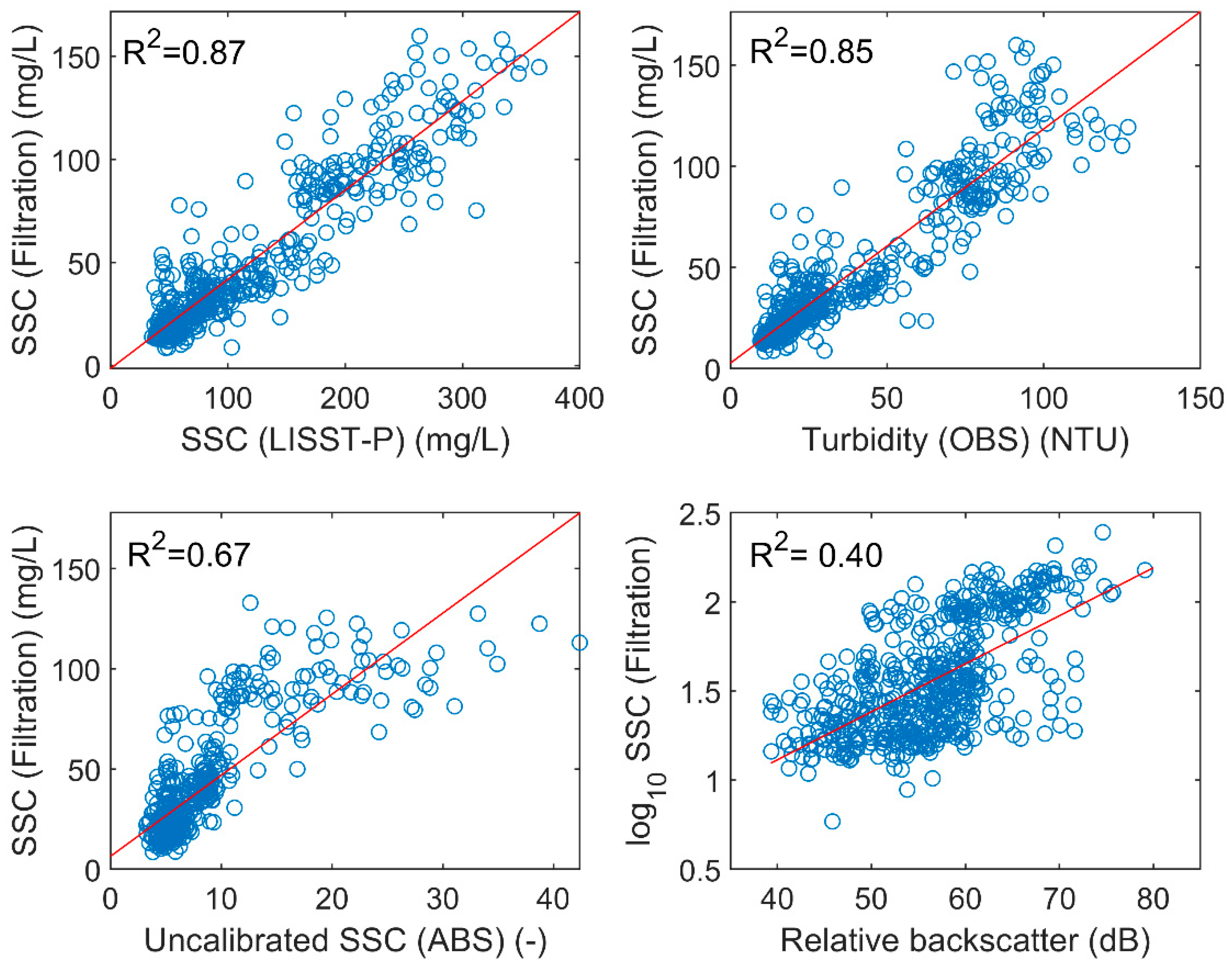
Before performing the comparative analysis of the indirect methods, the calibration based on the reference laboratory data was carried out for each of them. For this purpose, considering the theoretical background of the methods, we applied linear regression in each case. The correlation between the examined methods (Figure 2) is very good (the coefficient of determination (R2) is higher than 0.80) in the case of both the optical devices (LISST-Portable|XR and VELP TB1 portable turbidimeter) and satisfactory (R2 = 0.40–0.67) in case of the acoustic devices (LISST-ABS and ADCP). These results suggest that using indirect methods could indeed be an efficient alternative option of suspended sediment analysis methods. A thorough investigation of the indirect methods was performed, which consisted of an individual statistical analysis of the linear regression models and the comparative analysis of the indirect methods.
The uncertainties of the examined indirect methods were quantified via different statistical indicators. The predicted values were calculated using simple linear regression models and were compared with the observed values of SSC using the filtration method assuming that the direct analysis method is the most reliable. The statistical measures of the simple linear regression were considered according to [53,54,55]. The coefficient of determination (R2) indicates the adequacy of a regression model. The mean absolute error (MAE) is an average of the absolute errors (i.e., the difference between the predicted and the observed values). The mean absolute percentage error (MAPE) is a measure of prediction accuracy. The root-mean-square error (RMSE) is also a frequently used measure of the difference between values predicted by a model and the values observed. The %RMSE is the RMSE expressed as a percentage. The percent bias (PBIAS) measures the average tendency of the predicted data to be larger or smaller than observed values. It also measures over and underestimation of the bias and expresses it as a percentage. The thresholds of statistical measures are determined in [54,55]. Thus, the regression is good if 0.80 < R2, MAPE < 20, RMSE < 20%, and PBIAS < 10%. Table 1 shows the detailed interpretation of these statistical parameters which was used for the evaluation.
The individual statistical analysis of the examined indirect methods is based on the observed SSC values from the direct filtration methods and the calibrated values in case of each indirect method. The evaluation of the statistical measures is supplemented by graphical assessment of the scatter plots.
2.6. Comparative Analysis of Indirect Methods
Besides the previously presented individual statistical analysis, the comparison of the indirect methods was also carried out. However, considering the potential measurement errors in the physical laboratory analysis and the robustness of the tested laser diffraction instrument, we decided to improve the calibration of the methods based on the LISST-Portable|XR data instead of the filtration results. It was assumed that, in this way, the coarse errors resulted from human mistakes in the complex laboratory analysis, and can be filtered from the large dataset. After the recalibration process, the sediment concentration values from each analysis procedure were compared and a linear regression was fitted on the data pairs, using the least-squares approach. The regressions were assessed according to the R2 values and the visual agreement between the corresponding calibrated and observed (by the LISST-Portable|XR) values (i.e., graphical assessment).
3. Results
3.1. Individual Analysis of Methods
The results of the individual statistical analysis introduced in 2.5 are given in Table 2.
The calibrated ADCP backscatter proved to be the least satisfactory method—none of the statistical measures are satisfactory. Though the R2 of the LISST-ABS is good, the percentage errors (MAPE and %RMSE) are only satisfactory. The statistical results of the optical devices (LISST-Portable|XR and VELP TB1 turbidimeter) are good (R2 and PBIAS) and satisfactory (MAPE and %RMSE). According to this, calibrating the optical devices and the LISST-ABS is a reliable method, but the ADCP calibration needs to be examined more closely.
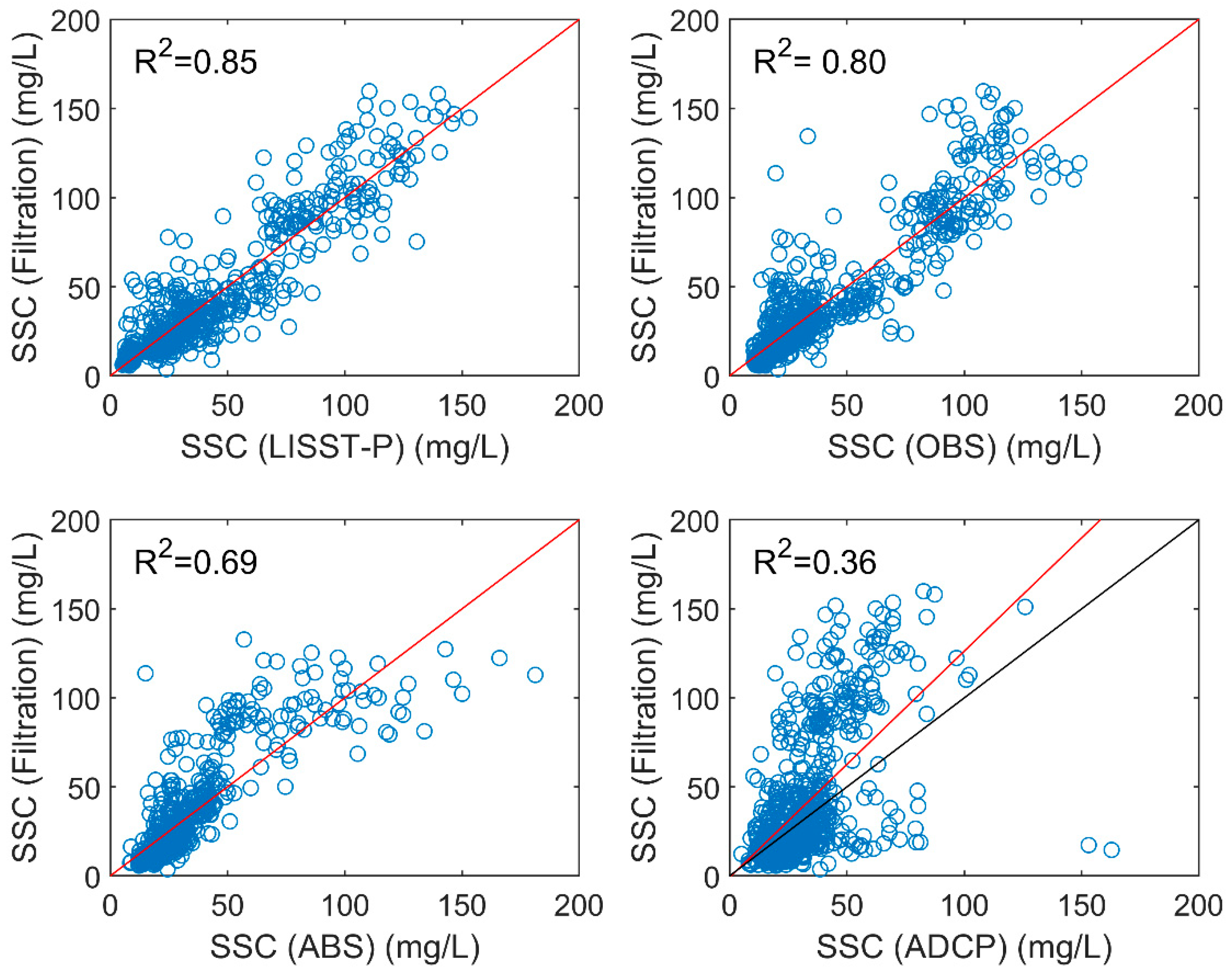
For a better understanding, the indirectly measured values related to the reference values are plotted in Figure 3. For instance, the “PBIAS can give a deceiving rating of model performance if the model overpredicts as much as it underpredicts, in which case PBIAS will be close to zero” [55] (p. 10) even though the prediction is not very good. This is the case with the LISST-ABS and the turbidimeter. The LISST-ABS, in general, tends to overpredict the SSC, while in the high SSC range (above 100 mg/L) this changes to underestimation. In the case of the turbidimeter, over and underestimation is balanced evenly. Although there are evidently more underestimated values, they are balanced by higher deviation in the overpredicted values. In contrast, the LISST-Portable|XR provides a relatively good prediction of actual SSC, just a slight overestimation can be observed, but the PBIAS value is higher than the PBIAS of the previously discussed methods. The unsatisfactory PBIAS of the ADCP is supported by the graphical visualisation—the calibrated SSC values clearly overestimate the observed SSC values.
3.2. Comparative Analysis
The results of the comparative analysis of the indirect methods presented in 2.6 are illustrated in Figure 4.
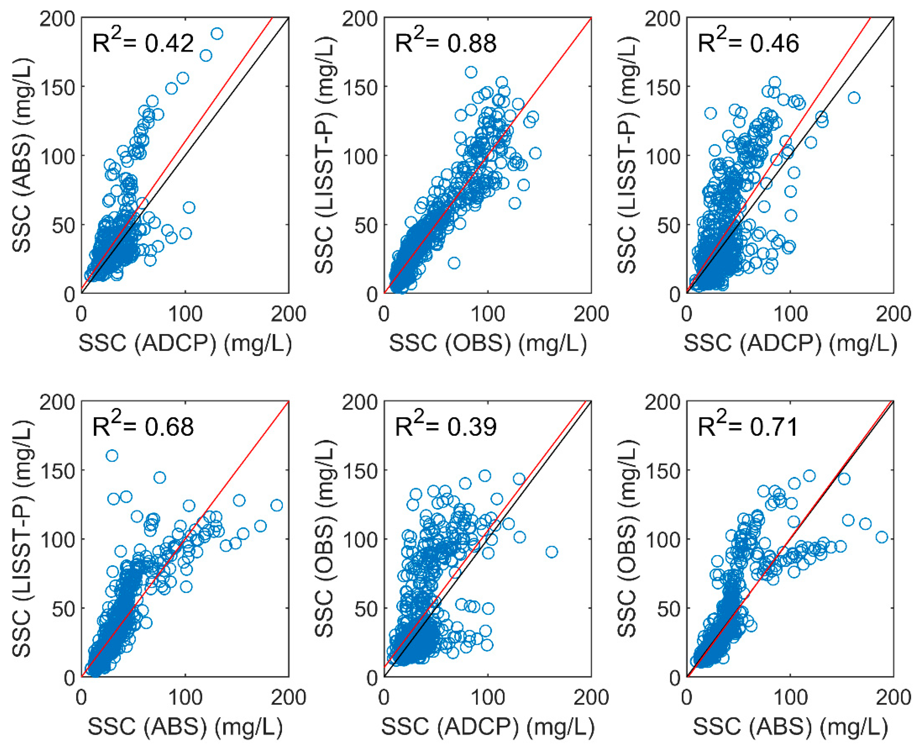
Comparing the acoustic methods, the relationship is only satisfactory (R2 = 0.42). The LISST-ABS values are higher than the ADCP values. This difference is probably due to the complex calibration procedure of the ADCP backscatter. Figure 4 suggests that another relationship should be established above 50 mg/L SSC.
Regarding the optical methods, the relationship is very good (R2 = 0.88). However, a larger scatter can be observed in higher SSC ranges (above ca. 100 mg/L). The volume of the standard vial of the portable turbidimeter is only 10 mL, which is not quite representative when the SSC of the analysed sample is high, and the sample is not continuously mixed during the analysis procedure. Another difference between the methods is that the OBS devices cannot take into account the inhomogeneity of the PSD, so the presence of coarser particles can introduce errors into the analysis. In contrast, the LISST-Portable|XR detects a wide range of particle size from 0.34 to 500 µm and the 117 mL sample is continuously mixed during the analysis, which does not let coarse particles settle.
When comparing the acoustic and optical methods, the relations are only satisfactory (R2 = 0.39–0.46) and good (R2 = 0.68–0.71). It is important to remember that the optical analyses were done in the laboratory, where the physical samples were analysed. The in situ LISST-ABS data is also from the measurement points, but the corresponding ADCP RB data was extracted from the fixed-boat ADCP backscatter measurements that were post-processed along the vertical. The relationship between the ADCP and the LISST-Portable|XR is rather scattered, the R2 is only 0.46. Figure 4 suggests that a separated calibration (e.g., according to the SSC or water discharge) should be examined in this case, too. In case of the LISST instruments, the fitted curve of basic linear regression coincides with the identity line, the R2 is equal to 0.68. The relationship is stronger in the range of low and average SSC, but the scatter increases above 50 mg/L. A possible explanation for this could be that, according to the manufacturer [47], the LISST-ABS is more sensitive in the range of the average suspended sediment particle size in the Danube (i.e., 20 µm). As expected from the strong regression between the LISST-Portable|XR and the turbidimeter, the relationship between the ADCP and the turbidimeter is similar to the one between the ADCP and the LISST-Portable|XR. However, the scatter is larger, and the coefficient of determination is lower (R2 = 0.39). The relationship between the LISST-ABS and the turbidimeter is the strongest within the acoustic–optical comparison (R2 = 0.71). The relationship is strong up to 50 mg/L but above that, the dataset divides into two parts. A possible explanation lies in the different sampling procedures: while the LISST-ABS measures in situ for an average of 30–40 s, the turbidimeter analyses a 10 mL sample from the whole sample volume that was taken during that time. The higher the SSC, the more difficult it is to prepare a representative sample for the turbidimeter analysis.
4. Discussion
4.1. Discussion of Indirect Methods
Although acoustic and optical methods have been widely applied in SSC measurements and their applications and limitations have been investigated and summarised, we claim that this comparative analysis of the four selected methods could provide a comprehensive practical guide in addition to the theoretical examples. Moreover, the results are based on the analysis of more than 1000 samples, which, we assume, means an adequately representative dataset.
Based on our experience, the LISST-Portable|XR is fundamentally easy to use, provided the analysts do their job with due care. With the right choice of the optical model and physical settings, after pouring the well-homogenised sample into the mixing chamber (it is important to avoid the formation of bubbles), the automated analysis is performed within three to five minutes. It has the great advantage of providing information on PSD as well. Theoretically, it would be suitable for field use [41], but the experience gained during this research project has shown that it is extremely sensitive to temperature conditions (precisely, the difference between the temperature of the mixing chamber and the water sample to be analysed). Depending on the typical particle size, the range of sediment concentration that can be analysed also varies [41]. According to the laboratory analysis of samples in a relatively wide SSC range, we found that at low (<10 mg/L) and high (>300–500 mg/L) concentrations in the Danube, the reliability of the results is significantly reduced (in comparison: in the case of glass beads with the same particle size as the suspended sediment in the Danube (i.e., 20 µm), this range would be 85–1063 mg/L [41]). While in the former case nothing can be done, in the latter case dilution can improve the analysis conditions. However, this range (10–500 mg/L) covers the SSC range of this section of the Danube efficiently.
The LISST-Portable|XR was compared with the direct filtration method in [43]. In the study carried out by Rai and Kumar [43], 61 samples were analysed within a wide range of SSC (68–1374 mg/L), and the determined linear regression between the SSC values is very good (R2 = 0.93). However, the scatter increased above 500 mg/L. In comparison, we analysed 604 samples in the range of 10–365 mg/L SSC. We found a similar relationship between the investigated values, namely, that the mass concentration determined by the LISST-Portable|XR is ~2.6 times higher than the filtrated values. The accuracy of the fitted linear regression is still very good (R2 = 0.85).
The portable turbidimeter is also suitable for field measurement due to its compactness. It is easy to handle, and the analysis procedure is fast (about 1 min). A small sample of water is enough for the measurement, but the representativeness of the results is questionable. However, the good correlation between the turbidity and the filtration values over the entire studied SSC range indicates that the turbidimeter performs well under the given circumstances (i.e., SSC range, suspended sediment, and water properties, etc.) of this study. The uncertainty is further increased by the fact that the glass vial must be perfectly spot-free and that the colour of the sample may affect the results (e.g., in streams containing significant amounts of organic matter). These experiences regarding the uncertainties meet the limitations presented in [20,23].
The OBS instruments are widely tested, and the turbidity units can be reliably converted to mg/L, e.g., [27,35,36,44]. Thus, we only intend to discuss in more detail, how the results of the comparison of optical devices (LISST-Portable|XR and VELP TB1 turbidimeter) complement previous studies. Rai and Kumar [44] recently tested the LISST-Portable|XR and a nephelometric turbidimeter, also. While they analysed 142 samples within the range of 0–600 NTU, we compared 771 results in the range of 0–130 NTU. Both comparisons resulted in a good correlation (R2 = 0.90 [44] and R2 = 0.88). Although the relationships are similar, it should be noted that the optical properties (e.g., colour) of the investigated rivers (the Tosh River in India [44] and the Danube River) are different.
From a practical point of view, the LISST-ABS seems to be the most suitable of the investigated instruments to replace the conventional direct methods. This indirect method requires no physical sampling (hence no laboratory analysis) and provides instantaneous, uncalibrated, and discrete concentration values. Thus, this automated measurement technique can also be used for quasi-continuous vertical and cross-sectional profiling. It is easy to handle and requires minimal post-processing (displaying results, filtering values when necessary, etc.). We found that this method is less reliable above ~50 mg/L SSC. The LISST-ABS measurements are expected to be sensitive to particle sizes within the range of the Danubian suspended sediment size, according to [48]. Knowing that the mean SSC along the studied section of the Danube is ~30 mg/L [39], the LISST-ABS can be considered a well-applicable method in continuous SSC monitoring.
The LISST-ABS and the LISST-Portable|XR were compared in [49]. The study site was selected in the Budapest area of the Danube which is located between the two study sites of this study. However, they covered a relatively narrow SSC range (~120–170 mg/L) with 40 samples, and we could extend the relationship between the two methods in a wider range (10–150 mg/L), based on the analysis of 621 samples with similar R2 (R2 = 0.57 [49] and R2 = 0.68).
Calibration of the ADCP backscatter is extremely useful as this instrument is often used for flow and velocity measurements, so obtaining additional information from the ADCP measurements is an important task. The theoretical background of calibration is well-established [26,27,29]—the calibration itself is complex but easy to perform. As a result, it requires more time than the other methods, but the additional information content of the resulting cross-sectional SSC distribution is undoubtedly the highest. With this method, even complex phenomena (e.g., mixing in river confluence zone [56]) can be investigated, or for example, resuspension of the bed material can be clearly seen during flood events. As discussed above, the calibration may depend on local conditions [32], and sediment characteristics. For instance, the effects of differentiation between fine and coarse suspended sediment particles are illustrated in [57]. Thus, the question arises, for example, as to how the inhomogeneous sediment can be taken into account at, for instance, the confluence of two rivers which differ significantly in the quality of suspended sediment (e.g., mineral composition [28] or organic sediment content).
The application of the ADCP backscatter calibration has been also tested in the context of SSC measurements in the Danube. The R2 of previous calibrations, e.g., in [51,56], indicate that the relationship with R2 = 0.36 (as a result of the analysis of 750 measurements) could be strengthened.
Furthermore, in accordance with [27], we found that the scatter between the ADCP and the turbidimeter increases above ~50 mg/L.
Table 3 summarises the selected attributes of the investigated indirect methods based on our experience along with the manufacturers’ information about accuracy and range.
4.2. Optimisation of Fluvial Suspended Sediment Monitoring
One of the objectives of this study was to propose a more efficient way of fluvial suspended sediment monitoring based on the investigation of selected indirect methods. Monitoring along large rivers such as the Danube often requires cooperation between several organisations (or even countries), which can be facilitated by harmonising the suspended sediment monitoring techniques. It is also important that monitoring itself includes a high spatial and temporal resolution of the selected parameters. Within a recent transnational programme called DanubeSediment, the sediment monitoring along the Danube River was evaluated and recommendations were made in order to improve water and sediment management as well as the morphology of the Danube River [18]. The optimisation presented here takes into account those practices and combines them with the findings of this comparative assessment of selected indirect methods. Recognising the applicability and limitations of these alternative and advanced methods, the reliability of the spatiotemporal characterisation of the relevant parameters of the suspended sediment transport can be enhanced.
As there are different types of temporal variation of suspended sediment transport parameters (e.g., according to flood regimes, interannual trends, and seasonality [9]), the temporal resolution of the monitoring should be as high as possible. An efficient method is the installation of a backscatter sensor (either ABS or OBS) near the bank in a representative cross section of the monitored river section. When calibrated properly, these instruments proved to be reliable [22,25]. As they measure the backscatter continuously, the temporal resolution is impeccable and the nature of changes in SSC can be monitored even during floods. A technical consideration is that the ABS is less sensitive to biofouling and algae blooming than the OBS [48]. However, the additional infrastructure (e.g., power supply, property protection, or data transfer) must be carefully designed [18].
The calibration of the fixed instruments is usually carried out by establishing the relationship between the value of the sensor and the results of a direct laboratory analysis of physical samples taken in the measurement point which is being monitored. This is extended by expeditionary cross-sectional measurements as well so that the cross-sectional SSL can be also determined. A thorough calibration procedure examines the relationships regarding different water regimes as well. However, the calibration procedure must be repeated to involve the potential hydromorphological changes at the monitoring site.
The direct laboratory analysis is often cumbersome and time-consuming. We investigated different indirect methods in order to prove their suitability as alternative options of the traditional direct methods. Well-calibrated optical devices such as the LISST-Portable|XR and the VELP TB1 turbidimeter could be a suitable alternative of direct methods [19,22]. We also found that these instruments can be calibrated reliably. If laboratory analysis of physical samples collected during low or mean water conditions is needed, these optical methods are highly recommended. However, the optical instruments prove to be less reliable for the analysis of samples collected during floods (i.e., when the SSC is above ~300 mg/L). Moreover, the LISST-Portable|XR determines the PSD as well. Although the monitoring of PSD is usually only of secondary importance, the information content of changes over time in PSD is not negligible. For instance, it may indicate a new source of fluvial sediment and the variation in PSD during flood events [59,60] is also required for the modelling of sediment transport processes.
The expeditionary cross-sectional measurements help to explore the spatial distribution of the SSC which is not negligible when selecting the position of a fixed sensor. The calibrated cross-sectional backscatter distribution of ADCP provides a detailed picture of the local suspended sediment conditions [51,56]. However, our results indicate that the calibration of the ADCP backscatter itself depends on the SSC (and hence, the water regime) so a thorough calibration procedure is required before using the ADCP for determining the cross-sectional distribution of the SSC. The cross-sectional profile of the SSC in the depth of the fixed instrument can easily be obtained by the calibrated LISST-ABS (or with appropriate cell sizing, also by the ADCP). Integrating this profile, the cross-sectional SSL can be determined more simply as well.
Taking advantage of the ADCP measurements, the installed backscatter sensor should be supplemented by a side-looking or horizontal ADCP (H-ADCP). This instrument has a wide range regarding the sampled area (a few hundred m [61]) so depending on the width of the cross section, the water discharge and the SSC distribution of a horizontal layer can also be determined by it (an application example is in [57]).
Part of our rationale was to provide a clear guide on which of the investigated methods to use and when to use them, in order to help optimise the suspended sediment transport monitoring along large rivers such as the Danube. While exact ranges (i.e., in SSC or particle size) of applicability could not been determined, it is evident that acoustic and optical methods can support optimised monitoring systems through a spatiotemporally enhanced way of collecting information about the parameters and characteristics of the suspended sediment transport. With the LISST-ABS and the ADCP, continuous measurements can be carried out which allow us to explore the spatial distribution of the SSC. Moreover, this information can be used for determining the distribution of the physical sampling points when multi-point sampling campaigns must be done in order to (re)calibrate the near-bank sensor. In contrast, the investigated optical methods can be reliably used in the laboratory. Since the time required for the analysis is far less than it is in case of the traditional direct methods, the optical methods prove to be very efficient.
4.3. Further Tasks
Although this study focused on quantifying the uncertainties of indirect methods, these errors are a result of the combined effects of sampling errors and uncertainties of analysis procedures. The most important task would be to perform a thorough sensitivity analysis regarding the effects of particle size, as this plays a major role in each indirect method [20,22,23]. The LISST-Portable|XR measures the particle size and determines the concentration (volume and mass) accordingly, and the sonar equation used for calibrating the ADCP backscatter takes into account the effects of particle size with the sediment attenuation coefficient, but the size effects should be directly analysed in the case of the LISST-ABS (which is highly sensitive within the average particle size range of the Danube [48]) and the turbidimeter as there is no differentiation between fine and coarse sediment particles.
In case of the LISST-Portable|XR, the setting of the optical model is also planned to be thoroughly tested. If some information is already provided about the sediment material, it is often better to choose the Mie scattering model [21,41]. However, the suspended sediment in the Danube along the Hungarian section is composed of four to five minerals in equal proportions. The inhomogeneity in the mineral composition leads to various densities, the refractive index, and the shape of the different minerals affect light scattering [23]. It has been experienced during the laboratory analysis that the LISST-Portable|XR is highly sensitive to the temperature differences, i.e., analysing cold samples, the PSD shows the presence of coarser particles—this is presumably caused by the forming of flocs due to the low temperature even when the ultrasonic probe was used for particle dispersion. Moreover, this also complicates the field application. Thus, the temperature-sensitivity of the LISST-Portable|XR should also be investigated.
The effects of the sample colour [20,23] regarding the optical devices could not yet be examined either. This is related to the composition of the suspended sediment as the colour often indicates the presence of organic matter. Algae blooming can also affect the transmission and turbidity of water.
Another question arises when calibrating the ADCP backscatter. The low values of R2 suggest that the calibration dataset should be carefully considered: hopefully, better values can be achieved if the calibration is carried out according to several SSC (or water discharge) ranges. The way in which the calibration should be spatially extended can also be examined: is it enough to use one calibration per river, or is it necessary to calibrate each section, cross section, or even measurement campaign?
5. Conclusions
This paper presented the comparative analysis of four indirect methods (optical methods: LISST-Portable|XR and VELP TB1 turbidimeter and acoustical methods: LISST-ABS and ADCP backscatter calibration) of fluvial SSC measurement based on the analysis more than 1000 samples. An attempt was made to statistically analyse the uncertainties of indirect methods to support the statement that the indirect methods could be adequate alternatives of the conventional direct methods (such as filtration). The results showed that applying laser diffraction, even in the field, is a straightforward way to determine SSC from water samples, however, it was also shown that the calibration of the optical sensor is crucial. Moreover, laser diffraction provides information on the PSD which supports the understanding of the sources of fine sediment. The herein tested laser diffraction method is, however, not applicable for continuous monitoring, but for expeditionary surveys. On the other hand, the results clearly demonstrate that acoustic backscatter sensors are a good alternative for pointwise, continuous suspended sediment measurements, thus, they can be applied as a basic element of a sediment monitoring system. Compared to optical backscatter sensors, which, based on our results, are still very efficient for detecting SSC, the acoustic sensors are more robust and require less maintenance during the operation, as the instrument is much less exposed to biofouling. This study underlined the applicability of the acoustic Doppler profilers for the spatial assessment of the suspended sediment transport, however, the weaker correlation compared to the other methods suggested that repeated calibration of the backscatter signal at expeditionary surveys of different measurement circumstances cannot be avoided.
The quantitative assessment of the tested indirect SSC measurement methods strongly supports the appropriate selection of the most suitable instruments for the different elements of a sediment monitoring system. Moreover, the practical characterisation summarised in Table 3 can greatly contribute to the improvement of existing suspended sediment monitoring stations and the establishment of new sediment monitoring stations. Even though the experiments were based on a high number of samples, further tests are still required, especially in the high concentration range, where the acoustic methods indicated weaker fit with the optical methods.
Author Contributions
F.P. participated in the field data collection and performed all the laboratory analysis and post-processing of the sediment data. F.P. prepared the relevant part of this manuscript. S.B. leads the related part of the funding project, designed the field measurement protocol, participated in the field measurements and reviewed the manuscript. All authors have read and agreed to the published version of the manuscript.
Funding
This research was partly funded by the project entitled “Drinking water: multidisciplinary assessment of secure supply from the source to the consumers” (project nr. 2018-1.2.1-NKP-2018-00011) supported by the National Research, Development and Innovation Office. The second author acknowledges the support of the ÚNKP-19-4 New National Excellence Program of the Ministry for Innovation and Technology and the Bolyai János fellowship of the Hungarian Academy of Sciences. This research was partly supported by MTA TKI of the Hungarian Academy of Sciences. Support of grant BME FIKP-VÍZ by EMMI is also kindly acknowledged. The authors acknowledge the funding of the OTKA FK 128429 grant.
Conflicts of Interest
The authors declare no conflict of interest.
References
- Landers, M.N. Fluvial Suspended Sediment Characteristics By High-Resolution, Surrogate Metrics of Turbidity, Laserdiffraction, Acoustic Backscatter, and Acoustic Attenuation. Ph.D. Thesis, Georgia Institute of Technology, Atlanta, GA, USA, 2012. [Google Scholar]
- Park, J.; Batalla, R.J.; Birgand, F.; Esteves, M.; Gentile, F.; Harrington, J.R.; Navratil, O.; López-Tarazón, J.A.; Vericat, D. Influences of Catchment and River Channel Characteristics on the Magnitude and Dynamics of Storage and Re-Suspension of Fine Sediments in River Beds. Water 2019, 11, 878. [Google Scholar] [CrossRef] [Green Version]
- Queensland Government. What Causes Streambed Erosion? Fact Sheet. 2001. Available online: https://www.qld.gov.au/__data/assets/pdf_file/0033/67677/what-causes-stream-bed-erosion.pdf (accessed on 10 February 2020).
- Koczka Bara, M.; Velísková, Y.; Dulovičová, R.; Schügerl, R. Influence of surface water level fluctuation and riverbed sediment deposits on groundwater regime. J. Hydrol. Hydromech. 2014, 62, 177–185. [Google Scholar] [CrossRef] [Green Version]
- Hauer, C.; Leitner, P.; Unfer, G.; Pulg, U.; Habersack, H.; Graf, W. The Role of Sediment and Sediment Dynamics in the Aquatic Environment. In Riverine Ecosystem Management, 1st ed.; Schmutz, S., Sendzimir, J., Eds.; Springer: Cham, Switzerland, 2018; Volume 8, pp. 151–169. [Google Scholar]
- Goldschneider, A.A.; Haralampides, K.A.; MacQuarrie, K.T.B. River sediment and flow characteristics near a bank filtration water supply: Implications for riverbed clogging. J. Hydrol. 2007, 344, 55–69. [Google Scholar] [CrossRef]
- Gillefalk, M.; Massmann, G.; Nützmann, G.; Hilt, S. Potential Impacts of Induced Bank Filtration on Surface Water Quality: A Conceptual Framework for Future Research. Water 2018, 10, 1240. [Google Scholar] [CrossRef] [Green Version]
- Nones, M. Dealing with sediment transport in flood risk management. Acta Geophys. 2019, 67, 677–685. [Google Scholar] [CrossRef] [Green Version]
- Mossa, J. Sediment dynamics in the lowermost Mississippi River. Eng. Geol. 1996, 45, 457–479. [Google Scholar] [CrossRef]
- Mead, A.A.; Demas, C.R.; Ebersole, B.A.; Kleiss, B.A.; Little, C.D.; Meselhe, E.A.; Powell, N.J.; Pratt, T.C.; Vosburg, B.M. A water and sediment budget for the lower Mississippi-Atchafalaya River in flood years 2008–2010: Implications for sediment discharge to the oceans and coastal restoration in Louisiana. J. Hydrol. 2012, 432, 84–97. [Google Scholar] [CrossRef]
- Joshi, S.; Jun, X.Y. Recent changes in channel morphology of a highly engineered alluvial river—The Lower Mississippi River. Phys. Geogr. 2018, 39, 140–165. [Google Scholar] [CrossRef]
- Van Rijn, L.C. Sediment transport, part I: Bed load transport. J. Hydraul. Eng. 1984, 110, 1431–1456. [Google Scholar] [CrossRef] [Green Version]
- Nittrouer, J.A.; Best, J.L.; Brantley, C.; Cash, R.W.; Czapiga, M.; Kumar, P.; Parker, G. Mitigating land loss in coastal Louisiana by controlled diversion of Mississippi River sand. Nat. Geosci. 2012, 5, 534–537. [Google Scholar] [CrossRef]
- Nittrouer, J.A.; Viparelli, E. Sand as a stable and sustainable resource for nourishing the Mississippi River delta. Nat. Geosci. 2014, 7, 350–354. [Google Scholar] [CrossRef]
- Joshi, S.; Xu, Y.J. Assessment of suspended sand availability under different flow conditions of the Lowermost Mississippi River at Tarbert Landing during 1973–2013. Water 2015, 7, 7022–7044. [Google Scholar] [CrossRef]
- Gomez, B. Bedload transport. Earth Sci. Rev. 1991, 31, 89–132. [Google Scholar] [CrossRef]
- Joshi, S.; Xu, Y.J. Bedload and suspended load transport in the 140-km reach downstream of the Mississippi River avulsion to the Atchafalaya River. Water 2017, 9, 716. [Google Scholar] [CrossRef] [Green Version]
- DanubeSediment. Handbook on Good Practices in Sediment Monitoring, Approved Project Report. 2019. Available online: http://www.interreg-danube.eu/approved-projects/danubesediment/outputs (accessed on 31 December 2019).
- Agrawal, Y.C.; Pottsmith, H.C. Instruments for particle size and settling velocity observations in sediment transport. Mar. Geol. 2000, 168, 89–114. [Google Scholar] [CrossRef]
- Downing, J. Twenty-five years with OBS sensors: The good, the bad, and the ugly. Cont. Shelf Res. 2006, 26, 2299–2318. [Google Scholar] [CrossRef]
- Agrawal, Y.C.; Whitmire, A.; Mikkelsen, O.A.; Pottsmith, H.C. Light scattering by random shaped particles and consequences on measuring suspended sediments by laser diffraction. J. Geophys. Res. 2008, 113. [Google Scholar] [CrossRef] [Green Version]
- Gray, J.R.; Gartner, J.W. Technological advances in suspended-sediment surrogate monitoring. Water Resour. Res. 2009, 45. [Google Scholar] [CrossRef] [Green Version]
- Czuba, J.A.; Straub, T.D.; Curran, C.A.; Landers, M.N.; Domanski, M.M. Comparison of fluvial suspended-sediment concentrations and particle-size distributions measured with in-stream laser diffraction and in physical samples. Water Resour. Res. 2015, 51, 320–340. [Google Scholar] [CrossRef]
- Boss, E.; Sherwood, C.R.; Hill, P.; Milligan, T. Advantages and Limitations to the Use of Optical Measurements to Study Sediment Properties. Appl. Sci. 2018, 8, 2692. [Google Scholar] [CrossRef] [Green Version]
- Rai, A.K.; Kumar, A. Continuous measurement of suspended sediment concentration: Technological advancement and future outlook. Measurement 2015, 76, 209–227. [Google Scholar] [CrossRef]
- Thorne, P.D.; Vincent, C.E.; Hardcastle, P.J.; Rehman, S.; Pearson, N. Measuring suspended sediment concentrations using acoustic backscatter devices. Mar. Geol. 1991, 98, 7–16. [Google Scholar] [CrossRef]
- Gartner, J.W. Estimating suspended solids concentrations from backscatter intensity measured by acoustic Doppler current profiler in San Francisco Bay, California. Mar. Geol. 2004, 211, 169–187. [Google Scholar] [CrossRef]
- Moate, B.D.; Thorne, P.D. Interpreting acoustic backscatter from suspended sediments of different and mixed mineralogical composition. Cont. Shelf Res. 2012, 46, 67–82. [Google Scholar] [CrossRef]
- Agrawal, Y.C.; Hanes, D.M. The implications of laser-diffraction measurements of sediment size distributions in a river to the potential use of acoustic backscatter for sediment measurements. Water Resour. Res. 2015, 51, 8854–8867. [Google Scholar] [CrossRef] [Green Version]
- Guerrero, M.; Szupiany, R.N.; Amsler, M.L. Comparison of acoustic backscattering techniques for suspended sediments investigations. Flow Meas. Instrum. 2011, 22, 392–401. [Google Scholar] [CrossRef]
- Guerrero, M.; Rüther, N.; Szupiany, R.N. Laboratory validation of acoustic Doppler current profiler (ADCP) techniques for suspended sediment investigations. Flow Meas. Instrum. 2012, 23, 40–48. [Google Scholar] [CrossRef]
- Sassi, M.G.; Hoitink, A.J.F.; Vermeulen, B. Impact of sound attenuation by suspended sediment on ADCP backscatter calibrations. Water Resour. Res. 2012, 48, 1–14. [Google Scholar] [CrossRef]
- Guerrero, M.; Rüther, N.; Szupiany, R.; Haun, S.; Baranya, S.; Latosinski, F. The acoustic properties of suspended sediment in large rivers: Consequences on ADCP methods applicability. Water 2016, 8, 13. [Google Scholar] [CrossRef] [Green Version]
- Hawley, N. A comparison of suspended sediment concentrations measured by acoustic and optical sensors. J. Great Lakes Res. 2004, 30, 301–309. [Google Scholar] [CrossRef]
- Patino, E.; Byrne, M.J. Application of Acoustic and Optic Methods for Estimating Suspended—Solids Concentrations in the St. Lucie River Estuary, Florida; U.S. Geological Survey Scientific Investigations Report 2004–5028; USGS: Reston, VA, USA, 2004.
- Vousdoukas, M.I.; Aleksiadis, S.; Grenz, C.; Verney, R. Comparisons of acoustic and optical sensors for suspended sediment concentration measurements under non-homogeneous solutions. J. Coast. Res. 2011, 64, 160–164. [Google Scholar]
- Sirabahenda, Z.; St-Hilaire, A.; Courtenay, S.C.; van den Heuvel, M.R. Comparison of acoustic to optical backscatter continuous measurements of suspended sediment concentrations and their characterization in an agriculturally impacted river. Water 2019, 11, 981. [Google Scholar] [CrossRef] [Green Version]
- Sommerhäuser, M.; Robert, S.; Birk, S.; Hering, D.; Moog, O.; Stubauer, I.; Ofenböck, T. Developing the Typology of Surface Waters and Defining the Relevant Reference Conditions. Final Report. 2003. Available online: http://www.undp-drp.org/pdf/1.1_River%20Basin%20Management%20-%20Phase%201/1.1_UNDP-DRP_Typology%20of%20SW_116_fr.pdf (accessed on 12 February 2020).
- DanubeSediment. Analysis of Sediment Data Collected Along the Danube. Approved Project Report. 2019. Available online: http://www.interreg-danube.eu/approved-projects/danubesediment/outputs (accessed on 12 February 2020).
- BMFLUW. Schwebstoffe im Fließgewässer—Leitfaden zur Erfassung des Schwebstofftransports. Bundesministerium für Land- und Forstwirtschaft; Umwelt und Wasserwirtschaft, 2. Auflage; BMLFUW: Vienna, Austria; Available online: https://www.bmnt.gv.at/wasser/wasser-oesterreich/wasserkreislauf/Schwebstoffe_LF.html (accessed on 31 December 2019).
- LISST-Portable|XR Manual Version 1.3. Available online: http://www.sequoiasci.com/wp-content/uploads/2015/06/LISST-PortableXR-Manual-Version-1_3.pdf (accessed on 31 December 2019).
- Le, H.A.; Gratiot, N.; Santini, W.; Ribolzi, O.; Soares-Frazao, S.; Deleersnijder, E. Sediment properties in the fluvial and estuarine environments of the Mekong River. E3S Web Conf. 2018, 40, 05063. [Google Scholar] [CrossRef] [Green Version]
- Rai, A.K.; Kumar, A. Sediment monitoring for hydroabrasive erosion: A field study from Himalayas, India. Int. J. Fluid Mach. Syst. 2017, 10, 146–153. [Google Scholar] [CrossRef]
- Rai, A.K.; Kumar, A. Determination of the particle load based on detailed suspended sediment measurements at a hydropower plant. Int. J. Sediment Res. 2019, 34, 409–421. [Google Scholar] [CrossRef]
- Bogárdi, J. Sediment Transport in Alluvial Streams, 1st ed.; Akadémiai Kiadó: Budapest, Hungary, 1971; pp. 44–48. [Google Scholar]
- VELP TB1 Portable Turbidimeter Leaflet. Available online: https://www.velp.com/euronet/contenuti/image/thumb/VELP_TB1_Turbidimeter_Leaflet.pdf (accessed on 31 December 2019).
- LISST-ABS Acoustic Backscatter Sensor User’s Manual Version 1.4. Available online: http://www.sequoiasci.com/wp-content/uploads/2015/04/LISST-ABS-Users-Manual_v1.4.pdf (accessed on 31 December 2019).
- Agrawal, Y.C.; Slade, W.; Pottsmith, H.C.; Dana, D. Technologies and experience with monitoring sediments for protecting turbines from abrasion. IOP Conf. Ser. Earth Environ. Sci. 2016, 49, 122005. [Google Scholar] [CrossRef] [Green Version]
- Conevski, S.; Guerrero, M.; Rüther, N.; Baranya, S. Testing the LISST-ABS Capabilities and Verifying its Usage for Measuring Suspended Sediment Concentration in Large Rivers. In Proceedings of the Particle in Europe (PiE) Conference, Budapest, Hungary, 3–5 October 2016. [Google Scholar]
- Guerrero, M.; Di Federico, V. Suspended sediment assessment by combining sound attenuation and backscatter measurements–analytical method and experimental validation. Adv. Water Resour. 2018, 113, 167–179. [Google Scholar] [CrossRef]
- Baranya, S.; Józsa, J. Estimation of suspended sediment concentrations with ADCP in Danube river. J. Hydrol. Hydromech. 2013, 61, 232–240. [Google Scholar] [CrossRef] [Green Version]
- Rüther, N.; Aleixo, R.; Guerrero, M.; Sørås, S.; Stokseth, S. Towards an establishment of a rating curve for suspended sediment transport by means of ADCP measurements. E3S Web Conf. 2018, 40, 04024. [Google Scholar] [CrossRef]
- Helsel, D.R.; Hirsch, R.M. Simple Linear Regression. In Statistical Methods in Water Researches, 1st ed.; U. S. Geological Survey: Reston, VA, USA, 2002; pp. 221–263. [Google Scholar]
- Moriasi, D.N.; Gitau, M.W.; Pai, N.; Daggupati, P. Hydrologic and water quality models: Performance measures and evaluation criteria. Trans. ASABE 2015, 58, 1763–1785. [Google Scholar]
- Lewis, C.D. Industrial and business forecasting methods. J. Forecast. 1982, 2, 194–196. [Google Scholar]
- Pomázi, F.; Baranya, S.; Török, G.T. Mapping of Suspended Sediment Mixing at a Confluence Zone to Improve Sediment Monitoring of a Large River. In Proceedings of the Particle in Europe (PiE) Conference, Lisbon, Portugal, 14–17 October 2018. [Google Scholar]
- Venditti, J.G.; Church, M.; Attard, M.E.; Haught, D. Use of ADCPs for suspended sediment transport monitoring: An empirical approach. Water Resour. Res. 2016, 52, 2715–2736. [Google Scholar] [CrossRef]
- Workhorse Rio Grande ADCP Guide. Available online: http://www.teledynemarine.com/Documents/Brand%20Support/RD%20INSTRUMENTS/Technical%20Resources/Manuals%20and%20Guides/Workhorse/Rio%20Grande%20ADCP%20Guide_Sep13.pdf (accessed on 31 December 2019).
- Hejduk, L.; Banasik, K. Variations in suspended sediment grain sizes in flood events of a small lowland river. IAHS Publ. 2010, 337, 189–196. [Google Scholar]
- Shang, D.; Qin, R.; Xu, H.; Xu, C.; Sun, K.; Zhou, Y. Variation of Suspended Particles in the Bottom Layer of the East China Sea with Data from Seafloor Observatory. Sensors 2019, 19, 5156. [Google Scholar] [CrossRef] [PubMed] [Green Version]
- Workhorse H-ADCP Technical Specifications. Available online: http://www.teledynemarine.com/Lists/Downloads/hadcp_datasheet_lr.pdf (accessed on 31 December 2019).
Figure 1.
Case study areas in the Hungarian section of the Danube River at the settlements near Sződliget (north of Budapest) and Ráckeve (south).
Figure 1.
Case study areas in the Hungarian section of the Danube River at the settlements near Sződliget (north of Budapest) and Ráckeve (south).

Figure 2.
Calibration curves of the indirect (optical and acoustic) methods.

Figure 3.
Comparison of predicted and observed values of suspended sediment concentration (SSC).

Figure 4.
Results of comparison of indirect methods (the values of the Acoustic Doppler Current Profiler (ADCP) is calibrated by the sonar equation; the values of the LISST-ABS (Acoustical Backscatter Sensor) and VELP TB1 turbidimeter are calibrated by the equation of simple linear regression between them and the LISST-Portable|XR mass concentrations).


Table 1.
Interpretation of statistical measures used for evaluating uncertainties (thresholds are based on [54,55]).
| Statistical Measure | Interpretation | |||
|---|---|---|---|---|
| Very Good | Good | Satisfactory | Not Satisfactory | |
| R2 | 0.80< | 0.65–0.80 | 0.40–0.65 | <0.40 |
| MAPE | <10 | 10–20 | 20–50 | 50< |
| %RMSE | <10 | 10–20 | 20–50 | 50< |
| PBIAS | <1 | 1–10 | 10–20 | 20< |
| MAE | Lower the better; optimally 0 | |||
| RMSE | Lower the better; optimally 0 | |||
Table 2.
Results of statistical analysis of indirect methods.
| Statistic | ADCP | LISST-ABS | LISST-P | VELP TB1 |
|---|---|---|---|---|
| Nr. of meas. | 750 | 621 | 604 | 771 |
| R2 (-) | 0.36 | 0.69 | 0.85 | 0.80 |
| MAE (mg/L) | 19.57 | 10.89 | 9.48 | 9.29 |
| MAPE (%) | 57.86 | 40.88 | 28.23 | 29.11 |
| RMSE (mg/L) | 30.24 | 15.79 | 13.65 | 15.40 |
| %RMSE (%) | 76.46 | 45.84 | 31.73 | 40.12 |
| PBIAS (%) | 19.55 | 0.00055 | 0.00323 | 0.00001 |
Table 3.
Summary of selected attributes of the investigated indirect methods.
| Attribute | Acoustic | Optical | ||
|---|---|---|---|---|
| ADCP RB | LISST-ABS | LISST-P | VELP TB1 | |
| Time needed | Approx. 30 min 1 | Real-time | 3–5 min | 1 min |
| Field application (Y/N) | Yes (in situ) | Yes (in situ) | Limited (sensitive to the cold temperature) | Yes (off-site) |
| Measurement location | Continuous (suitable for vertical, horizontal and cross-sectional profiling) | Discrete (but suitable also for continuous vertical and horizontal profiling) | Point (discrete) | Point (discrete) |
| Automated measurement (Y/N) | Yes | Yes | No | No |
| Probability of errors | Low | Low | Medium | Medium |
| Source of errors | Manual calibration (e.g., extracting echo intensity profiles, determining calibration dataset) | No differentiation between fine and coarse particles | Setting of the optical method and the material of SS; bubbles | Limited volume; settling velocity of coarser particles |
| Sensitivity | Calibration | Particle size | Temperature, high SSC | Sample colour, dirty vial |
| Accuracy | ± 1.5 dB (relative measure) [58] | ± 30% (for particles 30 to 400 µm) [47] | ± 20% [41] | ± 2% (0–500 NTU) and ±3% (501–1000 NTU) [46] |
| Range | 80 dB (dynamic range) [58] | 1–30,000 mg/L (depending on particle size) [47] | 10–1900 mg/L (depending on particle size) [41] | 0–1000 NTU [46] |
| Calibration (Y/N) | Yes; complex | Yes; easy with linear regression | Yes; easy with linear regression | Yes; easy with linear regression |
| Unit of measurement | Echo intensity | Uncalibrated SSC | Mass concentration (mg/L) | Turbidity (NTU) |
| Handling | Easy | Easy | Easy, but a bit of practice needed | Easy |
| Postprocessing needs | High | Low | Low (only when PSD in m/m% is needed) | No |
| Bonus strengths | Always used | Can be easily used for cross-sectional and vertical profiling as well | Provides information about PSD | Compact, small sample volume is needed |
1 when calibrating manually.
© 2020 by the authors. Licensee MDPI, Basel, Switzerland. This article is an open access article distributed under the terms and conditions of the Creative Commons Attribution (CC BY) license (http://creativecommons.org/licenses/by/4.0/).
Share and Cite
MDPI and ACS Style
Pomázi, F.; Baranya, S. Comparative Assessment of Fluvial Suspended Sediment Concentration Analysis Methods. Water 2020, 12, 873. https://doi.org/10.3390/w12030873
AMA Style
Pomázi F, Baranya S. Comparative Assessment of Fluvial Suspended Sediment Concentration Analysis Methods. Water. 2020; 12(3):873. https://doi.org/10.3390/w12030873
Chicago/Turabian StylePomázi, Flóra, and Sándor Baranya. 2020. "Comparative Assessment of Fluvial Suspended Sediment Concentration Analysis Methods" Water 12, no. 3: 873. https://doi.org/10.3390/w12030873
Note that from the first issue of 2016, this journal uses article numbers instead of page numbers. See further details here.