Effects of Rainfall Spatial Distribution on the Relationship between Rainfall Spatiotemporal Resolution and Runoff Prediction Accuracy

Abstract

We studied how rainfall spatial distribution affects the relationship between rainfall spatiotemporal resolution and runoff prediction accuracy under real field conditions. We gathered radar rainfall and discharge data for three rainfall events. These rainfall-runoff events were then reproduced using a kinematic wave model. Modeling accuracy was estimated quantitatively using the Nash–Sutcliffe model efficiency coefficient and peak discharge ratio. Normalized root-mean-square error ($\mathrm{nRMSE}$), skewness ($S_k$), and second scaled spatial moment of catchment rainfall (${\delta }_2$) were employed to quantify rainfall spatial distribution characteristics. By relating the accuracy of modeling results to the rainfall spatial characteristics using various rainfall spatiotemporal resolutions, we found that the modeling results converged to a value as the $\mathrm{nRMSE}$, $\left|S_k\right|$ and $|1-{\delta }_2|$ decreased. That is, rainfall spatial distributions affect the relationship between lower limit of rainfall spatiotemporal resolution for runoff models and runoff prediction accuracy.

1. Introduction

Advances in measurement and computational techniques have enabled us to consider additional physical processes for accurate flood forecasting. As knowledge regarding rainfall-runoff processes has developed and the related technologies and models have continued to advance, significant research efforts have focused on the accuracy and uncertainty of model input data because the accuracy of rainfall-runoff modeling relies heavily on input data [1,2,3]. Among the many types of input data, rainfall data is not only one of the most critical factors affecting the accuracy of runoff prediction [4], but also one of the factors that produce the highest degree of uncertainty [5]. Therefore, many studies have been conducted to reduce the uncertainty originating from rainfall data. For example, Fraga et al. [2] recently investigated the effects of rainfall data uncertainty on the performance of hydrological models in a small basin (~10 km²).

A relatively new paradigm for rainfall measurement is currently under development. Rainfall radar indirectly measures rainfall intensity and can produce raster-type rainfall data with various spatial and temporal resolutions. Although such systems must be calibrated with data measured by point rainfall gauges on the ground, radar can capture rainfall spatial variation much more accurately than point rainfall gauges. Furthermore, raster rainfall information is desirable for physically-based distributed rainfall-runoff models. Runoff simulations with high rainfall spatial resolution (RSR) provide more accurate results than those with lower RSR [4,6,7].

In addition to the performance of rainfall measurement facilities and computational resources, the spatial variability of hydrological factors can also affect flood forecasting accuracy. Ogden and Julien [8], and Shah et al. [9] studied the effects of rainfall spatial variability on rainfall-runoff characteristics using physically-based runoff models. Recently, many studies on the effects of the spatial and temporal variation of rainfall on the hydrological modeling results for relatively small urban basins have been conducted [10,11,12,13,14]. These studies commonly reported that higher spatiotemporal resolution rainfall data resulted in more accurate prediction results at small urban basins. One of the reasons was that spatial and temporal rainfall aggregation could affect rainfall peak and intensity [11]. Kim and Kim [15] hypothesized that the minimum RSR for accurate runoff prediction depended on spatiotemporal rainfall variation. However, their study was strictly limited to idealized basin and rainfall conditions. The test basin was a small one-dimensional impervious plain with a constant slope and uniform roughness. The tested rainfall distribution only varied linearly in space and was invariant in time. However, variations in temporal resolution of rainfall data can affect modeling results as much as variation in spatial resolution [10,13,14]. Furthermore, the basin scale, rainfall spatial distribution, and intensity were unrealistic. Therefore, it is still questionable whether or not rainfall spatial distribution has a significant effect on the RSR and rain temporal resolution (RTR) required for accurate runoff prediction in natural environments. Under real conditions, various factors, such as rainfall, topography, infiltration, and roughness, vary diversely in space and time unlike the ideal conditions considered in previous studies.

Therefore, in this study, we investigated the effects of rainfall spatial distribution on the relationship between rainfall spatiotemporal resolution and runoff prediction accuracy under real midsize watershed conditions. In the following sections, we first describe the characteristics of the target basin and rainfall events. Next, a brief description of a physically-based modeling technique and the results for various rainfall spatiotemporal resolutions are presented. Finally, the effects of rainfall spatial distribution on the relationship between rainfall spatiotemporal resolution and flood prediction accuracy are analyzed.

2. Methods

2.1. Study Area

The study area, the Mihocheon watershed, is located in the northern area of the Geumgang watershed in the Republic of Korea (Figure 1). This watershed is characterized by the temperate climate of the middle latitudes with four distinct seasons. The average annual rainfall is 1290 $\mathrm{mm}$ and more than 60% of the average annual rainfall occurs during the rainy season in summer. The total area of the watershed is 1855 ${\mathrm{km}}^2$, with a composition of 46% forest, 43% agricultural land, 6% urban area, 3% grass, and 2% bare land. There are four stage-discharge gauging stations operated by the Ministry of Environment as shown in Figure 1. That is, we can assume that four sub-basins are embedded the Mihocheon watershed as shown in Figure 1. In this study, the largest sub-basin area is referred to as Hapgang (HG). The sub-basins bounded in red, green, and blue lines are referred to as Seokhwa (SH), Bukil (BI), and Cheongju (CJ), respectively. The areas of the Hapgang, Seokhwa, Bukil, and Cheongju basins are 1853 km² 1594 km², 908 km², and 168 km², respectively.

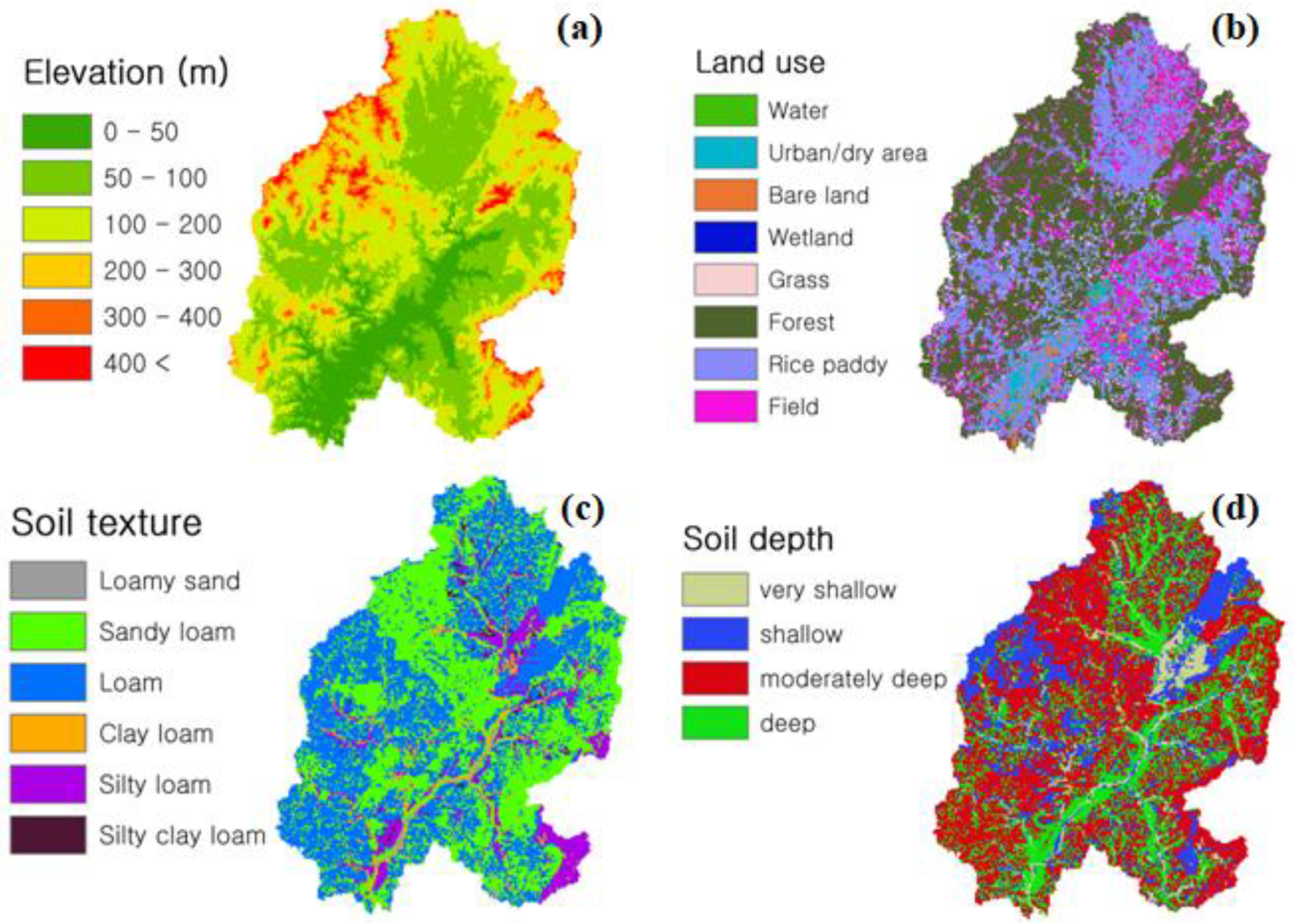
Hydrological data for this watershed, such as precipitation, water level, and discharge, are thoroughly measured and managed by the Korean government for the purposes of flood forecasting and drought management. The four stage-discharge gauging stations are located at the downstream ends of each basin as shown in Figure 1. The measured discharge values were converted from the measured water stage values using the rating curves at the stage-discharge gauging stations every 10 min. These data are regularly verified by the Ministry of Environment using a hydrological quality management system. Geographical features, such as digital elevation model (DEM) values, land use, soil texture, and soil depth (Figure 2 and

Table 1. Roughness coefficients for land use, soil depth, and soil texture geographical features.

Land Use	Classification	Roughness Coefficient	Impervious Ratio	Soil Depth	Classification		Soil Depth (cm)		Applied Soil Depth (cm)
	Water	0.030	1.000		Very shallow		0–20		10
	Urban/dry area	0.015	0.853
	Bare land	0.020	0.442		Shallow		20–50		25
	Wetland	0.070	1.000
	Grass	0.015	0.440		Moderately deep		50–100		75
	Forest	0.100	0.050
	Rice paddy	0.035	0.391		Deep		100–150		125
	Field	0.035	0.391
Soil Texture	Classification	Porosity (η)	Effective Porosity (θe)	Residual Moisture Content (θr)		Wetting Front Soil Suction Head (ψf) (cm)		Hydraulic Conductivity (K) (m/hr)
	Loamy sand	0.437	0.417	0.02		4.95		11.78
	Sandy loam	0.453	0.412	0.041		11.01		1.09
	Loam	0.463	0.434	0.029		8.89		0.34
	Clay loam	0.464	0.309	0.155		20.88		0.10
	Silty loam	0.501	0.486	0.015		16.68		0.65
	Silty clay loam	0.471	0.432	0.039		27.30		0.10

), are provided by the Ministry of Environment and the National Academy of Agriculture Science in Korea.

2.2. Storm Events and Radar Rainfall Data

The rainfall data used in this study were measured by a radar system at the Seodaesan Rainfall Radar Station, which is located near the Mihocheon watershed (Figure 1). This radar system uses the S-band and measures rainfall data with a 250 m grid size every 10 min. In addition to this radar station, eight rainfall-gauging stations are in operation inside the watershed and the rainfall gauge data are used to calibrate the radar rainfall data by the Ministry of Environment.

To examine the effects of rainfall spatial distribution on the relationship between rainfall spatiotemporal resolution and runoff prediction accuracy, we selected three rainfall events that occurred during the rainy season (

Table 2. Characteristics of rainfall events.

Storm Event	Period	Discharge Gauging Station	Mean Areal Rainfall (mm)	Max Rainfall (mm)	Min Rainfall (mm)
Event1	16–19 July 2017	Hapgang (HG)	178.3	286.2	21.9
		Seokhwa (SH)	188.2	286.2	72.7
		Bukil (BI)	174.7	279.4	78.1
		Cheongju (CJ)	197.4	286.2	72.7
Event2	24–27 July 2017	Hapgang (HG)	45.6	128.8	6.5
		Seokhwa (SH)	42.7	128.8	13.3
		Bukil (BI)	42.8	128.8	13.3
Event3	28–31 July 2017	Hapgang (HG)	29.1	94.4	0.2
		Seokhwa (SH)	33.3	94.4	2.9
		Bukil (BI)	36.2	94.4	9.6

). The mean areal rainfall for Event1 was approximately 185 mm for 3 days. This can be regarded as a heavy rainfall event. The mean areal rainfalls for Event2 and Event3 were approximately 30–45 mm over 2–3 days, representing mild rainfall events.

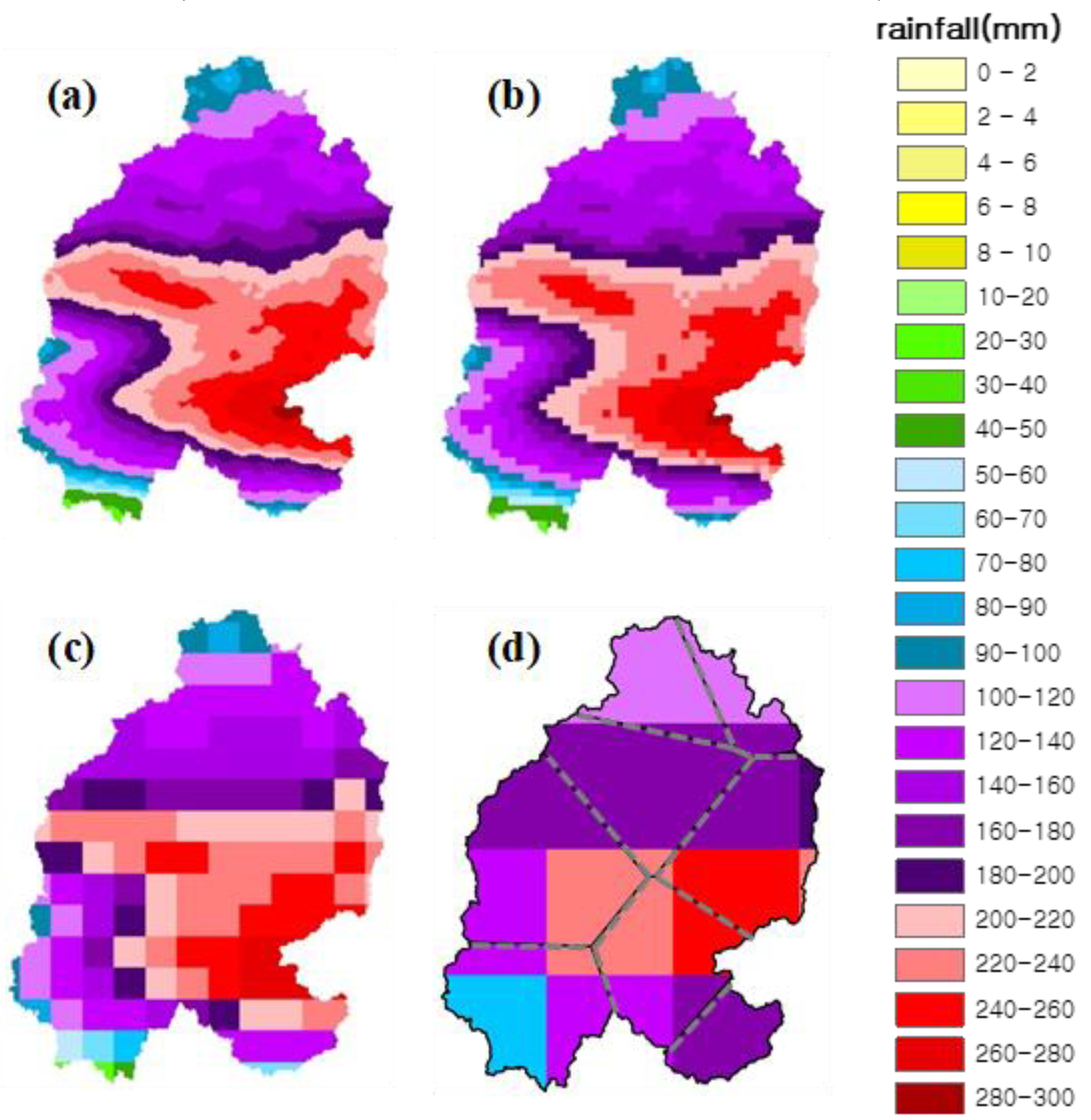
Because the radar station provided only $L_r$ = 250 m data, we generated low spatial resolution rainfall data by averaging the 250 m data. Considering that the average area of an element in the Thiessen network in Figure 3d is about 231 ${\mathrm{km}}^2$ and $\sqrt{231{\mathrm{km}}^2}\approx 15.2\mathrm{km}$, the largest $L_r$ was chosen to be $16\mathrm{km}$. Thus, the $L_r$ of radar rainfall data used for rainfall-runoff modeling were $L_r=250\mathrm{m}$, $500\mathrm{m}$, $1\mathrm{km}$, $2\mathrm{km}$, $4\mathrm{km}$, $8\mathrm{km}$, and $16\mathrm{km}$. Figure 3 presents several examples of rainfall distributions with various RSRs. During the prior test, we found that the shortest time to peak ($T_p$) of the tested cases was about 4 h at Cheongju basin. Thus, the time resolution ($T_r)$ of radar rainfall data used for the runoff modeling were $T_r=10\min$, $20\min$, $30\min$, and $60\min$ by considering the scale of $T_p$. As noted above, the radar system provides only $T_r=10\min$ data, thus the rainfall data with $T_r>10\min$ were generated by averaging the $T_r=10\min$ radar rainfall data. It needs to be noted that the radar measured data were not merged with rainfall gauge measurements on ground. Only the rainfall data measured by the radar station were used in this study.

2.3. Modeling Accuracy Estimation

To estimate the accuracy of the modeling results quantitatively, we employed the Nash–Sutcliffe model efficiency coefficient (NSE, Nash and Sutcliffe [16]) and peak discharge ratio (PE) as follows:

$$\mathrm{NSE}=1-\frac{\sum {\left(Q_e-Q_c\right)}^2}{\sum {\left(Q_e-\overline{Q_e}\right)}^2},$$

(1)

$$\mathrm{PE}=\frac{Q_c^p}{Q_e^p},$$

(2)

where $Q_e$ and $Q_c$ are the criterion and comparison discharges at the gauging stations, respectively. The overbar $\overline{\left(\right)}$ and superscript $p$ represent the average and peak values, respectively. According to the classification of Moriasi et al. [17], performance of hydrologic models is very good in the range of NSE = 1.0–0.8, good in the range of NSE = 0.8–0.6 and generally satisfactory in the range of NSE = 0.6–0.5. The range of NSE = 1.0–0.0 is an acceptable level.

2.4. Rainfall Spatial Variability Estimation

To characterize the differences between local and mean rainfall amounts quantitatively, normalized root-mean-square error (nRMSE) was calculated as follows:

$$\mathrm{nRMSE}=\sqrt{\frac{1}{n}{\sum }_{i=1}^n{\left(\frac{P_i-P_m}{P_m}\right)}^2},$$

(3)

where $P_i$ is the rainfall amount at a cell of the raster-type rainfall data, $P_m$ is the mean areal rainfall amount in the watershed, $i$ is the cell index, and $n$ is the total number of cells. The skewness ($S_k$) representing the degree of asymmetry of the rainfall spatial distribution about $P_m$ was calculated as follows:

$$S_k=\frac{\frac{1}{n}{\sum }_{i=1}^n{\left(P_i-P_m\right)}^3}{{\left[\frac{1}{n}{\sum }_{i=1}^n{\left(P_i-P_m\right)}^2\right]}^{3/2}},$$

(4)

To quantify the dependence between spatial rainfall organization, basin morphology, and runoff response, the second scaled spatial moments of the catchment rainfall [18] were calculated as follows:

$${\delta }_2=\frac{1}{g_2-g_1^2}\left[\frac{P_2}{P_o}-{\left(\frac{P_1}{P_o}\right)}^2\right],$$

(5)

$$P_n={\left|A\right|}^{-1}{\int }_A^{}{r}_t\left(x,y\right)d{\left(x,y\right)}^{n}dA,$$

(6)

$$g_n={\left|A\right|}^{-1}{\int }_A^{}d{\left(x,y\right)}^{n}dA,$$

(7)

where $d\left(x,y\right)$ is the distance between a position $\left(x,y\right)$ and the basin outlet along the flow path, $A$ is the spatial domain of the watershed, $P_n$ is the $n$-th spatial moment of the catchment rainfall, and $r_t\left(x,y\right)$ is the mean value of the time integrated rainfall at a location $\left(x,y\right)$. ${\delta }_2$ is the second scaled spatial moment of the catchment rainfall. Values of ${\delta }_2$ close to 1.0 indicate a relatively uniform rainfall distribution. Values of ${\delta }_2$ less than or greater than 1.0 indicate unimodal and multimodal rainfall distributions along the flow path, respectively. For consistent expression using $\mathrm{nRMSE}$ and $S_k$, we discuss spatial variability based on $|1-{\delta }_2|$ instead of ${\delta }_2$.

2.5. Rainfall-Runoff Modeling

For rainfall-runoff simulations, we utilized a grid-based rainfall-runoff model (GRM) based on a kinematic wave model [19]. The GRM can simulate surface runoff, infiltration, and subsurface flow, and consider control by hydraulic structures [20,21,22,23].

The GRM consists of a kinematic wave model for surface runoff on watersheds and river flows, and a Green–Ampt model for infiltration. The continuity equations for the GRM for overland and river flows are expressed as follows:

$$\frac{\partial h}{\partial t}+\frac{\partial q}{\partial x}=r-f+\frac{q_r}{\Delta y},$$

(8)

$$\frac{\partial h}{\partial t}+\frac{\partial q}{\partial x}=r-f+\frac{q_r}{\Delta y},$$

(9)

where $t$ is the time and $x$ is the horizontal axis. $h$ is the flow depth and $q$ is the discharge per unit width ($q=uh$), where $u$ is the flow velocity in the $x$ direction. $r$ is the rainfall intensity, $f$ is the infiltration rate, and $q_r$ is the return flow. $A_c$ is the cross-sectional river flow area, and $Q$ is the flow discharge of the river. $q_L$ is the lateral overland inflow, $q_{ss}$ is the subsurface flow into the channel, $q_b$ is the lateral inflow in the lower soil layer, and $\Delta y$ is the width of the control volume. The momentum equation for the GRM is expressed as

$$S_0=S_f,$$

(10)

where $S_0$ is the bottom slope and $S_f$ is the friction slope. Infiltration is calculated by the Green–Ampt model as follows [24]:

$$F\left(t\right)=Kt+\Delta \theta \psi ln\left(1+\frac{F\left(t\right)}{\Delta \theta \psi }\right),$$

(11)

$$f\left(t\right)=K\left(\frac{\Delta \theta \psi }{F\left(t\right)}+1\right),$$

(12)

where $F\left(t\right)$ and $f\left(t\right)$ are the cumulative infiltration and infiltration rate at time $t$, respectively. $\Delta \theta \left(=\left(1-S_e\right){\theta }_e\right)$ is the change in soil moisture content, where $S_e=\left(\theta -{\theta }_r\right)/\left(\eta -{\theta }_r\right)$ is the effective saturation, $\theta$ is the moisture content $({\theta }_r\le \theta \le \eta$), ${\theta }_r$($=\eta -{\theta }_e)$ is the residual moisture content, $\eta$ is the porosity, and ${\theta }_e$ is the effective porosity. $\psi$ is the wetting front soil head and $K$ is the hydraulic conductivity. The GRM assumes that the hydraulic gradient of subsurface flow is equal to the land surface gradient within a control volume based on the results presented by Beven (1981). It calculates the subsurface flow as follows:

$$q_{ss}=K{D}_{s}sin\left(S_a\right),$$

(13)

where $q_{ss}$ is the subsurface flow, $D_s$ is the saturated soil depth, and $S_a$ is the land surface slope. For subsurface flow modeling, the GRM divides soil layers into upper and lower layers. After the upper soil layer is saturated, percolation occurs in the lower soil layer and the percolation depth is calculated as

$$p=K_{Bv}\times \Delta t,$$

(14)

where $p$ is the percolation depth during $\Delta t$ and $K_{Bv}$ is the vertical hydraulic conductivity of the lower soil layer. The lateral inflow in the lower soil layer is calculated as follows [25]:

$$q_b=K_{Bh}{D}_B\sin \left(S_a\right),$$

(15)

where $K_{Bh}$ is the horizontal hydraulic conductivity in the soil layer and $D_B$ is the water depth in the soil layer. Additional details regarding the physics and numerical scheme of the GRM are described in the papers by Choi [19].

The computational grid size ($\Delta x$) and time step ($\Delta t$) for the GRM were always set to $\Delta x=250\mathrm{m}$ and $\Delta t=10\min$ because the computed discharges at the four gauging stations converged when $\Delta x=250\mathrm{m}$ and $\Delta t=10\min$. The rainfall-runoff modeling for the four sub-basins were simulated independently. That is, we assumed that there were four separate basins. Thus, for example, when we computed hydrographs at Seokhwa station, the downstream area of Seokhwa station was not considered and the hydrographs at Bukil and Cheongju stations were not calibrated.

The model parameters for simulation were calibrated by using the model-independent parameter estimation method for the runoff volume and peak discharge at the gauging stations with $L_r=\Delta x=250\mathrm{m}$ and $T_r=\Delta t=10\min$. It should be noted that the value of $\Delta x$ and $\Delta t$ for the GRM are different from the values of $L_r$ for RSR and $T_r$ for RTR, respectively.

To investigate the effects of RSR and RTR on modeling accuracy, we simulated ten rainfall-runoff events (Table 2) with seven different values of $L_r$ ($=250\mathrm{m}\mathrm{to}16\mathrm{km}$) and four different values of $T_r$ ($=10\min \mathrm{to}60\min$). Thus, total number of the tested cases was 280. Figure 4 presents the part of computed discharges among 280 cases, measured discharges and hyetographs measured by the radar station for the tested rainfall events. Each hydrograph has seven different computed results for the different RSRs and single $T_r=10\min$. As shown in Figure 4 and

Table 3. Nash–Sutcliffe model efficiency coefficient (NSE) and peak discharge ratio (PE) for runoff prediction with $L_r=250\mathrm{m}$ and $T_r=10\min$.

Case	Event1 (HG)	Event2 (HG)	Event3 (HG)	Event1 (SH)	Event2 (SH)	Event3 (SH)	Event1 (BI)	Event2 (BI)	Event3 (BI)	Event1 (CJ)
NSE	0.99	0.91	0.78	0.99	0.94	0.89	0.99	0.99	0.98	0.97
PE	1.00	1.00	1.00	1.00	1.00	1.00	1.00	0.99	1.00	1.00

, the computed discharges with $L_r=250\mathrm{m}$ and $T_r=10\min$ show very good agreement with the measured data. It needs to be noted that all the input rainfall data used in the numerical simulation were the radar data. The rainfall-gauging station data on ground were not used for the rainfall-runoff simulation.

3. Results and Discussion

3.1. RSR and RTR Effects on Runoff Prediction Accuracy

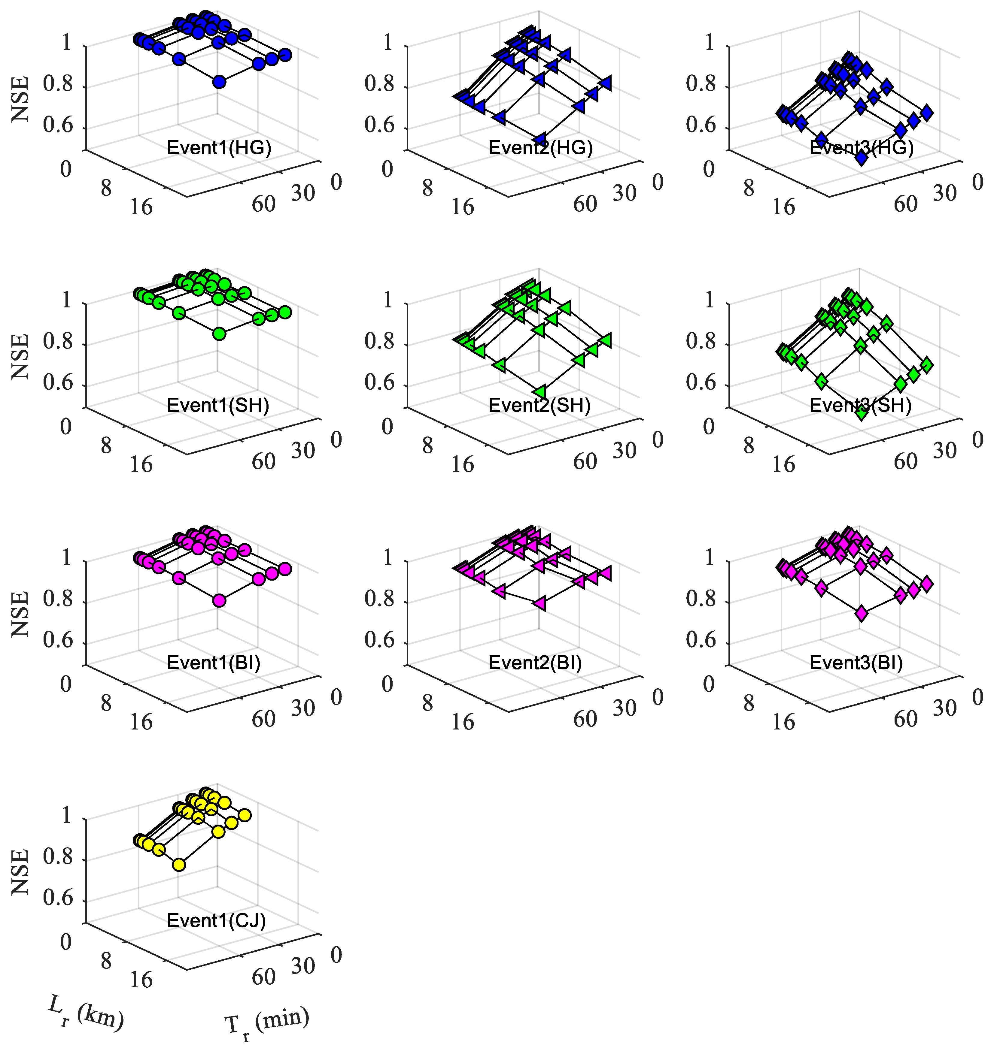
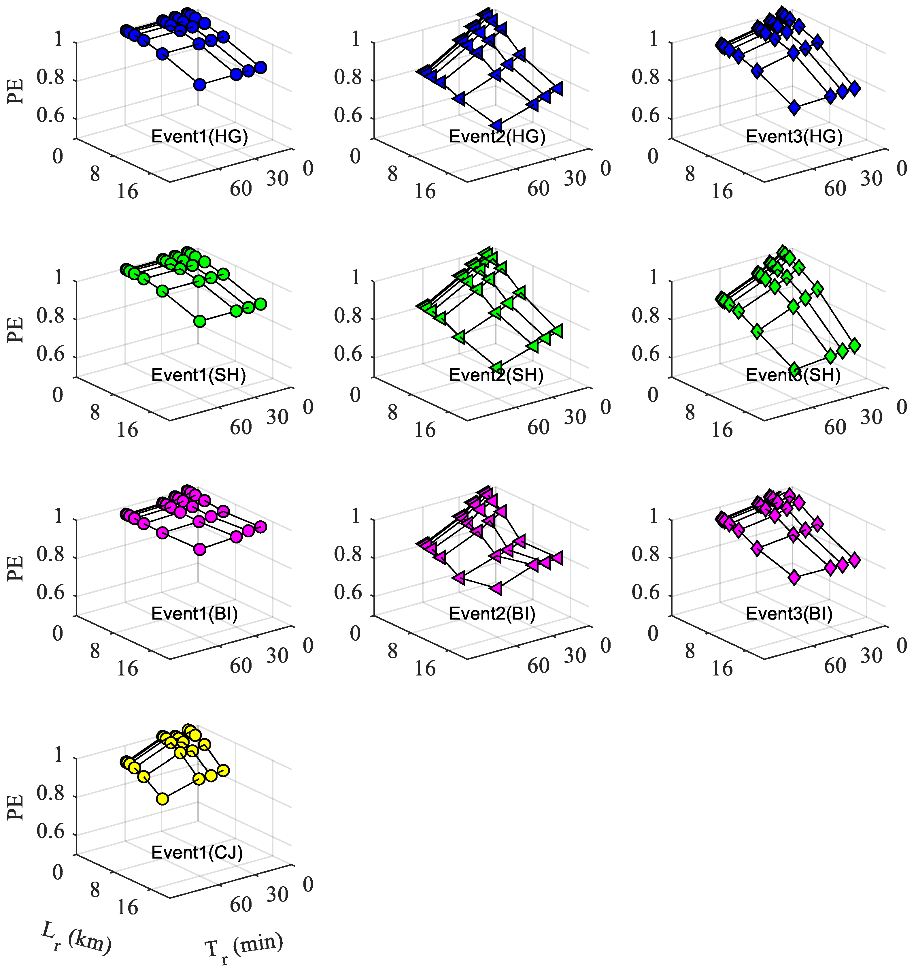
As shown in Figure 4, even when the available smallest value of $L_r$ and $T_r$ were used, some discrepancies between the measured and computed discharges were observed. These errors in the computed results with the smallest $L_r$ and $T_r$ and could not be resolved by changing $L_r$ and $T_r$ from $250\mathrm{m}$ and $10\min$ to other values, meaning there must be some error related to limitations of the GRM and the accuracy of input data. Therefore, the computed discharges using $L_r=250\mathrm{m}$ and $T_r=10\min$ were used as the criterion ($Q_e$) and the computed discharges with other combinations of $L_r$ and $T_r$ values were used as the comparisons ($Q_c$) for estimating the NSE and PE. All the estimated NSE and PE for various spatial and temporal resolutions are presented in Figure 5 and Figure 6.

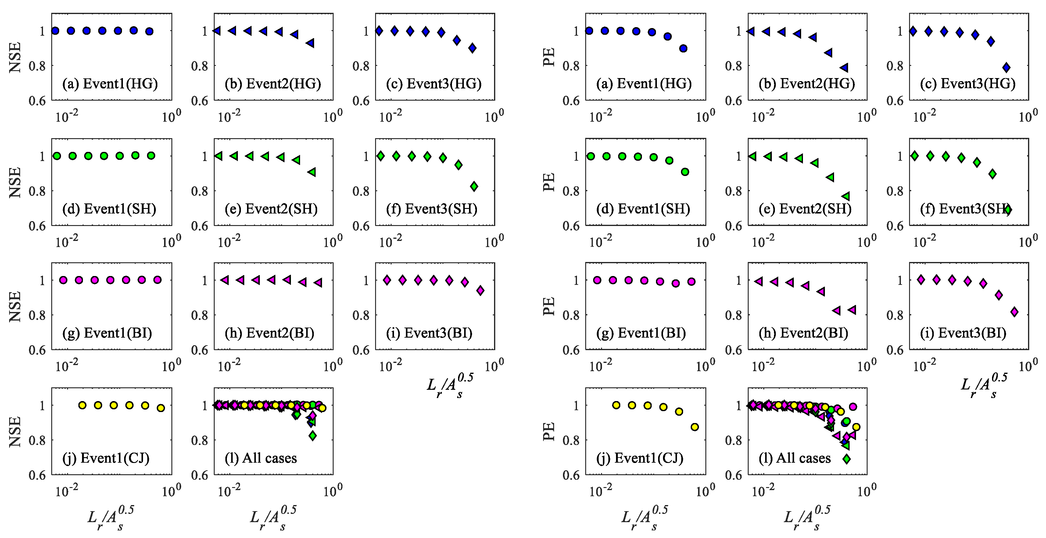
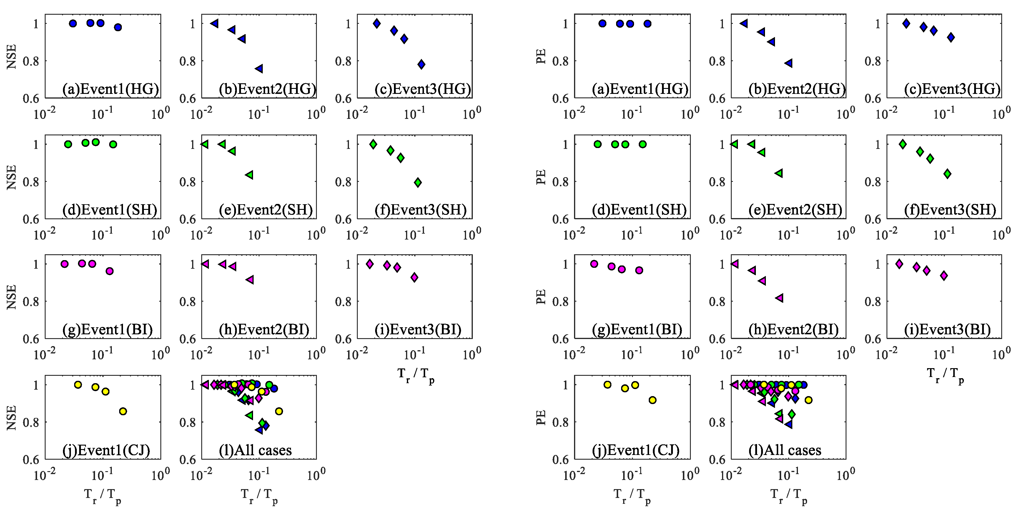
Figure 7 (Supplementary Materials) presents the NSE and PE of the computed discharges at the stage-discharge gauging stations with a fixed $T_r\left(=10\min \right)$ and seven values of $L_r\left(=250\mathrm{m}\sim 16\mathrm{km}\right)$ for the tested events. To account for accuracy of the spatial rainfall distributions in model input of fine and coarse resolutions relative to basin size, we used dimensionless form $L_r/\sqrt{A_s}$, where $A_s$ is the area of the sub-basins. As shown in this figure, higher RSR values (smaller $L_r/\sqrt{A_s}$ values) resulted in NSE and PE values closer to 1.0 compared to lower RSR values under real watershed conditions. For similar purpose, $T_r/T_p$ was employed to consider accuracy of the temporal rainfall variation in model input. Consistently with Figure 7, Figure 8 (Supplementary Materials) shows the NSE and PE of the computed discharges with various values of $T_r$ and a fixed $L_r\left(=250\mathrm{m}\right)$ for the tested events, where higher RTR values (smaller $T_r/T_p$ values) resulted in NSE and PE values closer to 1.0 compared to lower RTR values under real watershed conditions, as observed by [7,10,11,12,13,14,26,27,28]. These results indicate that convergence by $L_r$ and $T_r$ values must be verified in the view of rainfall input in addition to convergence by $\Delta x$ and $\Delta t$ in the view of numerical scheme for solving governing equations.

3.2. Effects of Rainfall Spatial Distribution on the Relationship between RSR and Prediction Accuracy

Figure 7 reveals that different rainfall events can result in different NSE and PE values, even when the same RSR is used for the same watershed. The NSE and PE of Event1 (HG) were different from the NSE and PE of Event2 (HG) when the same $L_r$ value was used for the same watershed. Because all factors other than rainfall characteristics were the same, the only factor that could have affected the NSE and PE values was the different rainfall characteristics of the individual rainfall events.

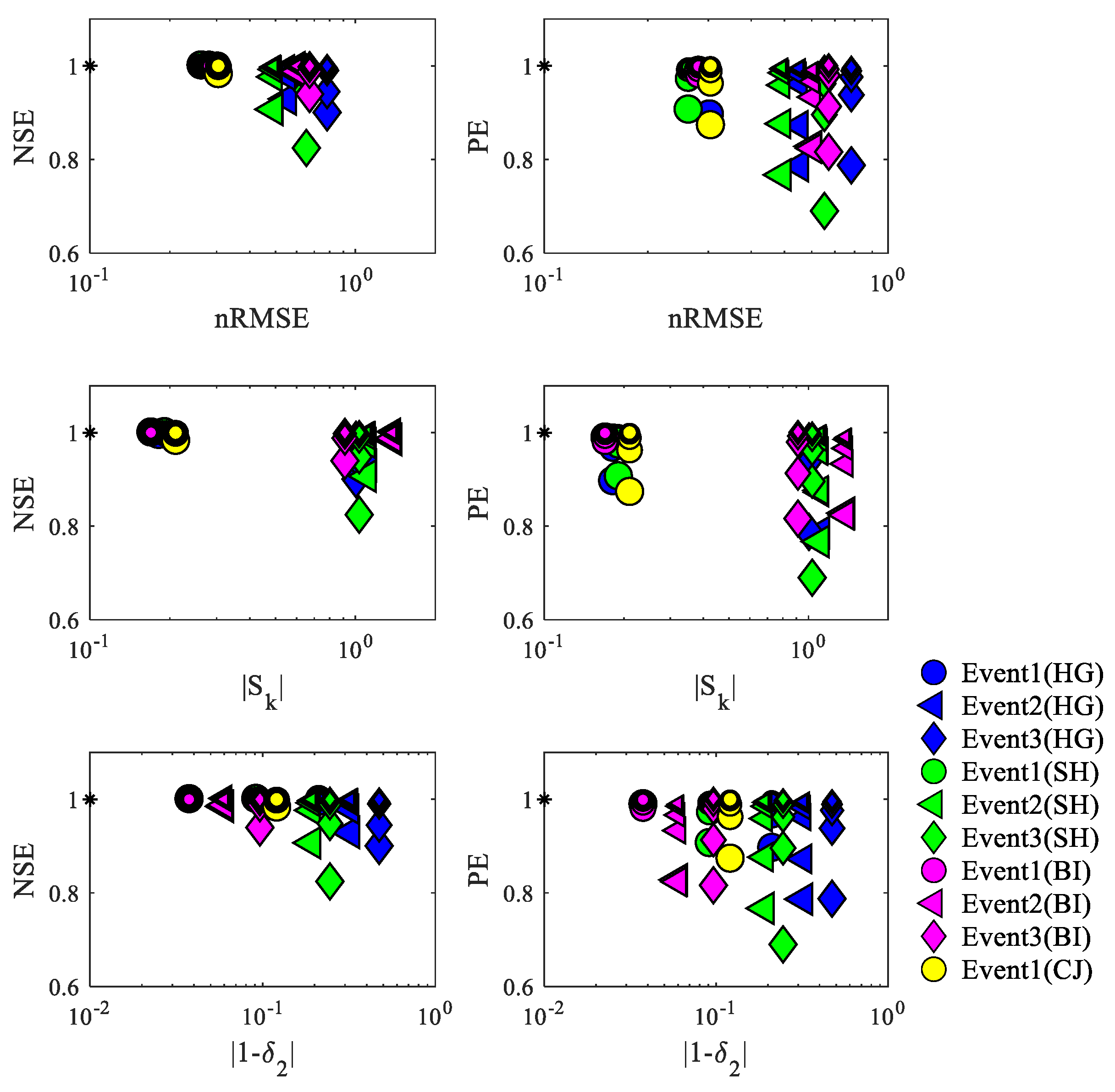
Figure 9 shows the relationship between rainfall spatial distribution characteristics ($\mathrm{nRMSE}$, $S_k$, and ${\delta }_2$) and sensitivity of modeling accuracy (NSE and PE) to RSR for the tested cases, where the NSE and PE would be $1.0$ when $\mathrm{nRMSE}$, $\left|S_k\right|$ and $|1-{\delta }_2|$ approach to zero like ∗ symbols in Figure 9 (and Figure 10). As shown in Figure 10, the sensitivity to the input RSR generally decreased as the rainfall spatial variabilities ($\mathrm{nRMSE}$, $\left|S_k\right|$, and $\left|1-{\delta }_2\right|$) increased. Wide range of the variability of NSE and PE indicates that prediction accuracy depends substantially on RSR of rainfall data. For this study, the prediction accuracy was less dependent on the RSR when the $\mathrm{nRMSE}$, $\left|S_k\right|$, and $\left|1-{\delta }_2\right|$ were small than when the $\mathrm{nRMSE}$, $\left|S_k\right|$, and $\left|1-{\delta }_2\right|$ were large. In other words, when the same value of RSR was used, the prediction accuracy increased as $\mathrm{nRMSE}$, $\left|S_k\right|$ and $|1-{\delta }_2|$ decreased. Therefore, it is evident that rainfall spatial variability affects the required RSR level for accurate runoff prediction. This indicates that computed results with large values of $L_r$ can converge if the values of $\mathrm{nRMSE}$, $\left|S_k\right|$, and $|1-{\delta }_2|$ are sufficiently small. However, one must utilize a sufficiently small value of $L_r$ to ensure that the computed results converge if the values of $\mathrm{nRMSE}$, $\left|S_k\right|$ and $|1-{\delta }_2|$ are large.

3.3. Effects of Rainfall Spatial Distribution on the Relationship between RTR and Prediction Accuracy

Consistent features with the effects of rainfall spatial distribution on the relationship between RSR and prediction accuracy were also observed from the relationship between RTR and prediction accuracy. Figure 8 shows that different NSE and PE values resulted from different rainfall spatial distributions, even when the same RTR was used for the same watershed. Thus, we can infer that the rainfall spatial characteristics also affect the relationship between RTR and prediction accuracy. This is because the only factor that affected the variations of the NSE and PE values at the same watershed in Figure 8 was the different rainfall characteristics of the individual rainfall events.

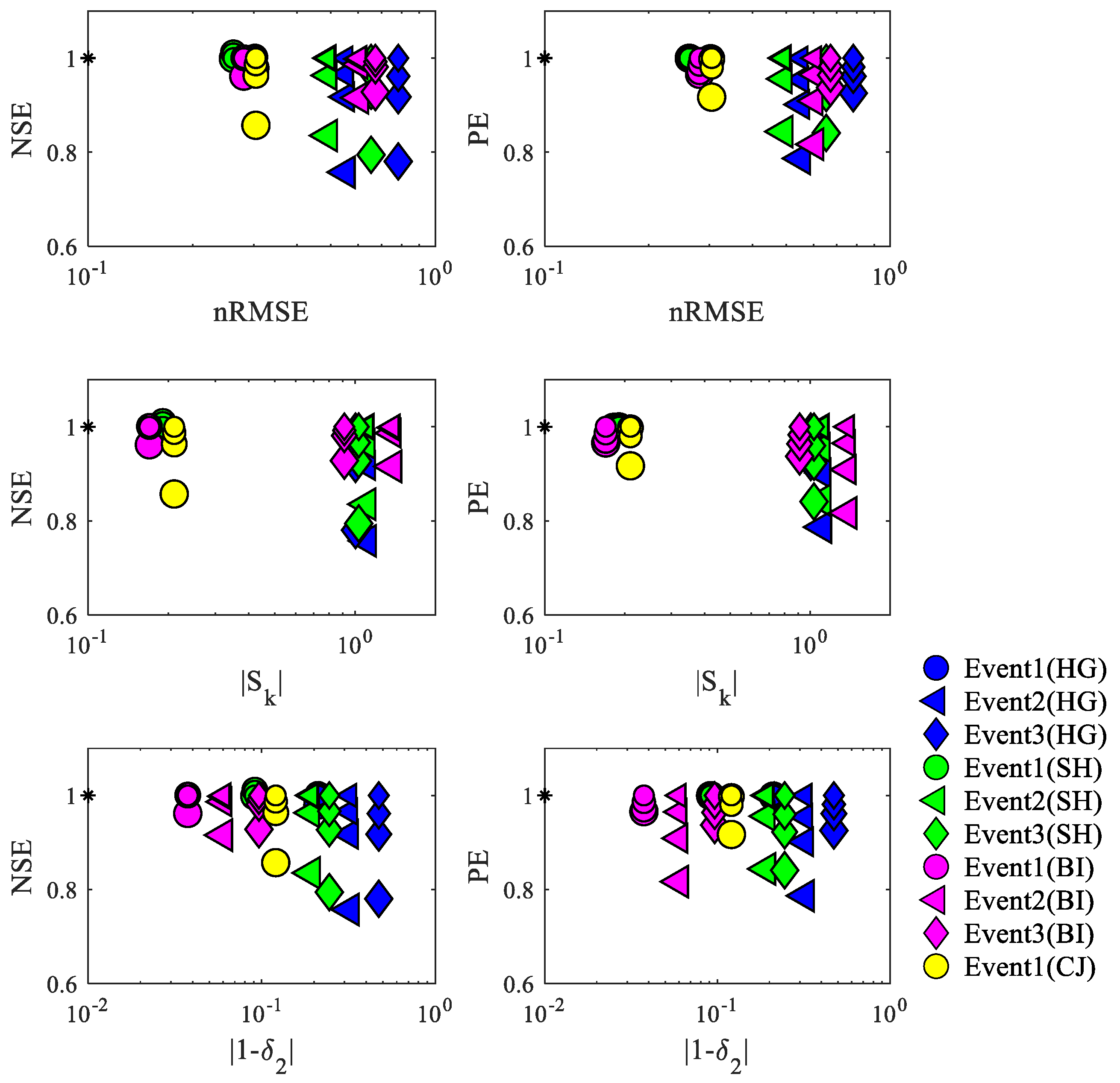
Figure 10 shows the relationship between rainfall spatial distribution characteristics ($\mathrm{nRMSE}$, $S_k$, and ${\delta }_2$) and sensitivity of modeling accuracy (NSE and PE) to RTR for the tested cases. As shown in Figure 10, the sensitivity to the input RTR generally decreased as the rainfall spatial variabilities ($\mathrm{nRMSE}$, $\left|S_k\right|$, and $\left|1-{\delta }_2\right|$) increased. Because wide range of the variability of NSE and PE indicates that prediction accuracy depends substantially on RTR of rainfall data, the prediction accuracy was less dependent on the RTR when the $\mathrm{nRMSE}$, $\left|S_k\right|$, and $\left|1-{\delta }_2\right|$ were small than when the $\mathrm{nRMSE}$, $\left|S_k\right|$, and $\left|1-{\delta }_2\right|$ were large. In other words, when the same value of RTR was used, the prediction accuracy increased as $\mathrm{nRMSE}$, $\left|S_k\right|$, and $|1-{\delta }_2|$ decreased. Therefore, it is evident that rainfall spatial variability affects the required RTR level for accurate runoff prediction, at least for the tested cases.

3.4. Application: Upper Limit for $L_r$ of Radar Rainfall Data

Because NSE and PE converge as $L_r$ decreases (Figure 4, Figure 5 and Figure 6), we can determine an upper limit for $L_r$ (lower limit for RSR) to ensure the required runoff prediction accuracy by setting a threshold.

Table 4. Upper limit of $L_r$ for the required peak discharge prediction accuracy for the Mihocheon watershed.

Storm Event	Upper Limit of Lr (km) for Required Accuracy with Tr = 10 and Tr = 30 (min)
	90% Accuracy		95% Accuracy		97% Accuracy		99% Accuracy
	Tr = 10	Tr = 30	Tr = 10	Tr = 30	Tr = 10	Tr = 30	Tr = 10	Tr = 30
Event1(HG)	16	16	8	8	8	8	4	2
Event2(HG)	4	0.25	4	-	2	-	1	-
Event3(HG)	8	8	4	0.25	4	-	1	-
Event1(SH)	16	16	8	8	8	8	4	4
Event2(SH)	4	2	4	-	2	-	2	-
Event3(SH)	4	2	4	-	2	-	2	-
Event1(BI)	16	16	16	16	16	4	16	-
Event2(BI)	4	0.5	2	-	2	-	1	-
Event3(BI)	8	4	4	2	4	-	1	-
Event1(CJ)	4	4	4	4	2	2	1	1
Minimum Lr (km)	4	0.25	2	<0.25	2	<0.25	1	<0.25

shows the upper limits for $L_r$ to ensure the required prediction accuracy based on $Q_p$ for the Mihocheon watershed. For example, to ensure a forecasting accuracy of 90%–95% for $Q_p$, an $L_r$ value of 2–4 $\mathrm{km}$ should be used if $T_r=10\min$. If a coarser temporal resolution $T_r=30\min$ is chosen, we cannot obtain higher than 95% accuracy for many cases as shown in Table 4 because the lower limit of the present radar system is $L_r=250\mathrm{m}$. Although we need further investigation with more many cases, this approach will be helpful to find reliable $L_r$ and $T_r$ for the area.

It is interesting to test the accuracy of the flood forecasting performed by the flood control office in the area. Currently, the flood control office mainly uses the Thiessen network presented in Figure 3d, where the area of an element in the Thiessen network is approximately equal to the area of a radar cell with $L_r=16\mathrm{km}$. Therefore, we can roughly assume that the peak flood prediction accuracy for the area operated by the flood control office using the Thiessen network would be less than 90% at most if the other conditions were the same.

4. Conclusions

We studied the effects of rainfall spatial distribution on the relationship between rainfall spatiotemporal resolution and runoff prediction accuracy under real watershed conditions. We collected the rainfall and discharge data from rainfall events in the Mihocheon watershed. These events were then reproduced using a kinematic wave model. Because the computed discharges converged when $\Delta x=L_r=250\mathrm{m}$ and $\Delta t=T_r=10\min$, we assumed that the modeling results with $\Delta x=L_r=250\mathrm{m}$ and $\Delta t=T_r=10\min$ represented the criteria for accurate rainfall-runoff modeling. Lastly, we investigated the effects of rainfall spatial distribution ($\mathrm{nRMSE}$, $S_k$, and ${\delta }_2$) on the lower limit of RSR and RTR for required runoff prediction accuracy. Several major findings are summarized below.

(1) The dependence on high spatial and temporal resolutions to achieve accurate prediction is proportional to $\mathrm{nRMSE}$, $\left|S_k\right|$ and $|1-{\delta }_2|$ in terms of quality. In other words, the computed results with a large value of $L_r$ and $T_r$ will converge if $\mathrm{nRMSE}$, $\left|S_k\right|$, and $|1-{\delta }_2|$ are sufficiently small. On the other hand, we need small value of $L_r$ and $T_r$ to ensure that the computed results will converge when $\mathrm{nRMSE}$, $\left|S_k\right|$ and $|1-{\delta }_2|$ are large. Therefore, we can conclude that rainfall spatial distribution has a significant effect on the required RSR and RTR for accurate runoff prediction under midsize real field conditions.

(2) For rainfall-runoff simulation, convergence by $L_r$ and $T_r$ of rainfall input data must be checked separately from the convergence by $\Delta x$ and $\Delta t$ for computational schemes of distributed rainfall-runoff models. It is strictly required to check the convergence of computed results depending on $\Delta x$ and $\Delta t$ for numerical schemes when we use grid-based numerical models. In addition, we need one more procedure to check the convergence depending on rainfall input resolution to assure reliability of rainfall-runoff modeling results.

(3) Even when the same RSR and RTR are used for the same watershed, different rainfall events with different characteristics can result in different NSE and PE. Therefore, when using radar, we must not only consider electrical or mechanical performance, but also rainfall spatial distribution (hydrological aspects) to determine the rainfall radar resolution for accurate flood forecasting.

In addition, the results presented in this paper can be used to remove a physically originating uncertainty in rainfall-runoff modeling. Although the results seem to introduce additional uncertainty into lumped runoff models because such models cannot accurately consider rainfall spatial distributions, the additional uncertainty is superior to ignorance.

Although we were able to find a clue for removing physically-originating uncertainty for rainfall-runoff modeling, various unknown factors still remain. In particular, the proposed results in this study are limited within one specific area. Thus we need further investigations based on sufficient cases with different climate, size, geographical features and topography in order to quantify effects of rainfall spatial distribution on relationship between rainfall resolution and prediction accuracy. Additionally, a better definition of quantity of rainfall temporal distribution needs to be developed [11], linking rainfall temporal variability to relationship between rainfall spatiotemporal resolution and accuracy of rainfall-runoff prediction.

References

- Arnaud, P.; Bouvier, C.; Cisneros, L.; Dominguez, R. Influence of rainfall spatial variability on flood prediction. J. Hydrol. 2002, 260, 216–230. [Google Scholar] [CrossRef]
- Fraga, I.; Cea, L.; Puertas, J. Effect of rainfall uncertainty on the performance of physically-based rainfall-runoff models. Hydrol. Process. 2018. [Google Scholar] [CrossRef] [Green Version]
- Moulin, L.; Gaume, E.; Obled, C. Uncertainties on mean areal precipitation: Assessment and impact on streamflow simulations. Hydrol. Earth Syst. Sci. Dis. 2009, 13, 99–114. [Google Scholar] [CrossRef] [Green Version]
- Beven, K. Kinematic subsurface stormflow. Water Resour. Res. 1981, 17, 1419–1424. [Google Scholar] [CrossRef]
- McMillan, H.; Krueger, T.; Freer, J. Benchmarking observational uncertainties for hydrology: Rainfall, river discharge and water quality. Hydrol. Process. 2012, 26, 4078–4111. [Google Scholar] [CrossRef]
- Beven, K.J. Rainfall-Runoff Modelling: The Primer; John Wiley and Sons: Hoboken, NJ, USA, 2011. [Google Scholar]
- Sangati, M.; Borga, M. Influence of rainfall spatial resolution on the flash flood modeling. Nat. Hazards Earth Syst. Sci. 2009, 9, 575–584. [Google Scholar] [CrossRef] [Green Version]
- Ogden, F.L.; Julien, P.Y. Runoff sensitivity to temporal and rainfall spatial variability at runoff plane and small basin scales. Water Resour. Res. 1993, 28, 2589–2597. [Google Scholar] [CrossRef]
- Shah, S.; O’Connell, P.; Hosking, J. Modelling the effects of spatial variability in rainfall on catchment response. 2. Experiments with distributed and lumped models. J. Hydrol. 1996, 175, 89–111. [Google Scholar] [CrossRef]
- Bruni, G.; Reinoso, R.; Van de Giesen, N.C.; Clemens, F.H.L.R.; Ten Veldhuis, J.A.E. On the sensitivity of urban hydrodynamic modelling to rainfall spatial and temporal resolution. Hydrol. Earth Syst. Sci. 2015, 19, 691–709. [Google Scholar] [CrossRef] [Green Version]
- Cristiano, E.; Ten Veldhuis, M.-C.; Gaitan, S.; Ochoa Rodriguez, S.; van de Giesen, N. Critical scales to explain urban hydrological response: An application in Cranbrook, London. Hydrol. Earth Syst. Sci. 2018, 22, 2425–2447. [Google Scholar] [CrossRef] [Green Version]
- Gires, A.; Onof, C.; Maksimovic, C.; Schertzer, D.; Tchiguirinskaia, I.; Simoes, N. Quantifying the impact of small scale unmeasured rainfall variability on urban runoff through multifractal downscaling: A case study. J. Hydrol. 2012, 442, 117–128. [Google Scholar] [CrossRef] [Green Version]
- Ochoa-Rodriguez, S.; Wang, L.P.; Gires, A.; Pina, R.D.; Reinoso-Rondinel, R.; Bruni, G.; Ichiba, A.; Gaitan, S.; Cristiano, E.; Van Assel, J.; et al. Impact of spatial and temporal resolution of rainfall inputs on urban hydrodynamic modelling outputs: A multi-catchment investigation. J. Hydrol. 2015, 531, 389–407. [Google Scholar] [CrossRef]
- Yang, L.; Smith, J.A.; Baeck, M.L.; Zhang, Y. Flash flooding in small urban watersheds: Storm event hydrological response. Water Resour. Res. 2016, 52. [Google Scholar] [CrossRef] [Green Version]
- Kim, C.; Kim, D.H. Effect of rainfall spatial distribution and duration on minimum spatial resolution of rainfall data for accurate surface runoff prediction. J. Hydro Environ. Res. 2018, 20, 1–9. [Google Scholar] [CrossRef]
- Nash, J.E.; Sutcliffe, J.V. River flow forecasting through conceptual models, Part I–A discussion of principles. J. Hydrol. 1970, 10, 282–290. [Google Scholar] [CrossRef]
- Moriasi, D.N.; Gitau, M.W.; Pai, N.; Daggupati, P. Hydrologic and water quality models: Performance measures and evaluation criteria. Trans. ASABE 2015, 58, 1763–1785. [Google Scholar]
- Zoccatelli, D.; Borga, M.; Viglione, A.; Chirico, G.; Bloschl, G. Spatial moments of catchment rainfall: Rainfall spatial organisation, basin morphology, and flood response. Hydrol. Earth Syst. Sci. 2011, 15, 3767–3783. [Google Scholar] [CrossRef] [Green Version]
- Choi, Y.S.; Choi, C.K.; Kim, H.S.; Kim, K.T.; Kim, S. Multi-site calibration using a grid-based event rainfall-runoff model: A case study of the upstream areas of the Nakdong River basin in Korea. Hydrol. Process. 2015, 29, 2089–2099. [Google Scholar] [CrossRef]
- Choi, Y.S.; Kim, K.T.; Lee, J.H. Development of grid based distributed rainfall-runoff model with finite volume method. J. Korea Water Resour. Assoc. 2008, 41, 895–905. [Google Scholar] [CrossRef] [Green Version]
- Choi, Y.S.; Shin, U.; Kim, K. Preliminary Study of Computational Time Steps in a Physically Based Distributed Rainfall–Runoff Model. Water 2018, 10, 1269. [Google Scholar] [CrossRef] [Green Version]
- Kim, N.; Shin, M. Estimation of Peak Flow in Ungauged Catchments Using the Relationship between Runoff Coefficient and Curve Number. Water 2018, 10, 1669. [Google Scholar] [CrossRef] [Green Version]
- Noh, S.J.; Choi, Y.; Choi, C.; Kim, K. Parameter estimation of a distributed hydrologic model using parallel PEST: Comparison of Impacts by Radar and Ground Rainfall Estimates. J. Korea Water Resour. Assoc. 2013, 46, 1041–1052. [Google Scholar] [CrossRef]
- Green, W.H.; Ampt, G.A. Studies on soil physics, part 1: The flow of air and water through soils. J. Agric. Sci. 1911, 4, 1–24. [Google Scholar]
- Freeze, R.A.; Cherry, J.A. Groundwater; Prentice-Hall: Englewood Cliffs, NJ, USA, 1979. [Google Scholar]
- Julien, P.Y.; Moglen, G.E. Similarity and length scale for spatially varied overland flow. Water Resour. Res. 1990, 26, 1832–1891. [Google Scholar] [CrossRef]
- Ogden, F.L.; Julien, P.Y. Runoff model sensitivity to radar rainfall resolution. J. Hydrol. 1994, 158, 1–18. [Google Scholar] [CrossRef]
- Rafieeinasab, A.; Norouzi, A.; Kim, S.; Habibi, H.; Nazari, B.; Seo, D.; Lee, H.; Cosgrove, B.; Cui, Z. Toward high-resolution flash flood prediction in large urban areas—Analysis of sensitivity to spatiotemporal resolution of rainfall input and hydrologic modeling. J. Hydrol. 2015, 531, 370–388. [Google Scholar] [CrossRef] [Green Version]
Figure 1.
Mihocheon watershed. Black thick line: Hapgang (HG) basin, red line: Seokhwa (SH) basin, green line: Bukil (BI) basin, and blue line: Cheongju (CJ) basin. Triangles: stage-discharge gauging stations. *: Rainfall radar station.
Figure 2.
Geographic data of the Mihocheon watershed. (a) Digital elevation model (DEM) elevations, (b) land use, (c) soil texture, and (d) soil depth. The cell size is 250 × 250 m.
Figure 3.
Rainfall distributions with various rainfall spatial resolutions (RSRs) during Event1: (a) , (b) , (c) , and (d) . Gray dashed lines in (d) represent the Thiessen network.
Figure 4.
Measured and computed runoff hydrographs with . Vertical cyan bar represents rainfall (mm).
Figure 5.
NSE values for runoff predictions with various RSRs and rain temporal resolution (RTRs).
Figure 6.
PE values for runoff predictions with various RSRs and RTRs.
Figure 7.
NSE and PE values for runoff predictions with various RSRs with .
Figure 8.
NSE and PE values for runoff predictions with various RTRs with .
Figure 9.
Relationship between variation of and by , and nRMSE, , and (with ). Symbol size is proportional to the from 250 m to 16 km.
Figure 10.
Relationship between variation of and by , and nRMSE, , and (with ). Symbol size is proportional to the from 10 min to 60 min.