Hydraulic Properties of a Cultivated Soil in Temperate Continental Climate Determined by Mini Disk Infiltrometer


Czech University of Life Sciences, Faculty of Agrobiology, Food and Natural Resources, Department of Water Resources, Kamýcká 129, 165 00 Praha 6—Suchdol, Czech Republic
*
Author to whom correspondence should be addressed.
Water 2020, 12(3), 843; https://doi.org/10.3390/w12030843
Submission received: 24 February 2020
/
Revised: 9 March 2020
/
Accepted: 13 March 2020
/
Published: 17 March 2020
(This article belongs to the Section Hydraulics and Hydrodynamics)
Abstract
:Hydraulic conductivity at and near saturation (Ks and K(h)) are among the most important characteristics defining water behavior in soil. Characterization of possibilities, advantages and limitations of the Mini Disk infiltrometer (MDI) for Ks and K(h) determination in comparison with Hood infiltrometer (HI) was the main aim of this study. The MDI device was subjected to testing on a cultivated silty clay loam soil under three different tillage treatments; conventional, reduced and no-tillage plot. The results are based on 72 infiltration experiments carried out during four experimental phases within one year. Steady-state and transient data analysis methods were applied. K(h) values were determined for van Genuchten hydraulic parameters taken from different sources (two versions of User’s manual, Rosetta). The results show suitability of MDI to determine K(h) of tested soil; clear differences have been observed between the K(h) values measured on plots with different tillage treatment. However, these values were significantly lower (ANOVA, α = 0.05) than those measured by HI. MDI based data were reflecting seasonal changes in structure and pore-size distribution with quantification of macropore contribution to the total saturated flux. Application of K(h) MDI data for fine-textured and structural soils evaluated before 2010 should be reconsidered.
1. Introduction
Hydraulic conductivity characterizes the ability of soil to infiltrate and transport water through the soil profile; saturated hydraulic conductivity Ks for the saturated soil and unsaturated hydraulic conductivity K(h) for the unsaturated soil. The soil texture and the soil structure are the characteristics defining the ability of soil to conduct water. The amount of conducted water is determined not only by the size and volumetric proportion of the pores, but also their geometric configuration given by their connectivity and tortuosity. These characteristics in a cultivated soil are subjected to changes in relation to the vegetation season and applied agrology, such as soil tillage treatment. If the soil is not able to infiltrate water, a surface runoff and soil erosion can occur. Many substances (e.g., pesticides, chemicals, contaminants) are transported with water through the soil profile. Thus, the hydraulic conductivity is a key parameter in practically all models dealing with water resources, environmental and health risk, soil erosion assessment, etc. In situ techniques can produce more representative values of hydraulic conductivity in comparison to laboratory measurements on soil core samples, as they characterize larger volume of soil in its natural state with the undisturbed pore network [1,2,3].
Standard methods for Ks and K(h) determination are presented in national technical standards (e.g., ASTM standards (American Society for Testing and Materials) [4,5], or ISO standard (International Organization for Standardization) [6]). The Ks and K(h) values are determined on the basis of some other measured characteristic which is functionally related to Ks and K(h). No reference method measuring directly the Ks or K(h) value exists and when comparing the results, the measurement method should be always provided. The Ks is in fact the maximal value of the speed of water moving through the soil profile, because all pores and fractures (macropores and preferential paths) can be full of water and participating in the water movement [7]. However, most of the field soil-water interactions is taking place in unsaturated soil, while the saturated state of the soil is only temporal.
There are several commercially available devices for K(h) determination in situ; i.e., Mini Disk infiltrometer (MDI, METER Group, Inc., Pullman, WA, USA), Tension infiltrometer with detachable membrane on 20 cm base (Eijkelkamp Soil&Water, The Netherlands or Soil Measurement Systems, USA), Tension infiltrometer with 8 cm non-detachable membrane (Soil Measurement Systems, Tucson, AZ, USA), and Hood infiltrometer (HI, Umwelt-Geräte-Technik, GmbH., Müncheberg, Germany). The efficiency and precision of the measurements can be improved by automatic data recording. Tension infiltrometers can employ differential pressure transducer to record water level heights in the reservoirs at pre-set time intervals [8]; similar automation was presented by Madsen and Chandler [9] for MDI, while Rodný et al. [10] automated the MDI on the basis of particle tracking principle.
MDI (originally by Decagon Devices, Inc.; now METER Group, Inc.) has been introduced to the market in 1997 and thanks to its low price, small dimensions and simplicity in use, has become a very popular device. The MDI is often employed as a simple tool for K(h) information for a single applied pressure head based on User’s manual guidelines (usually –2 cm) [9,11,12]. On the contrary, this paper is focused on specific details in K(h) determination by MDI considering its experimental settings and data evaluation options.
As reviewed by Angullo-Jaramillo et al. [13], the methods used for deriving the hydraulic conductivity from infiltration data obtained with tension infiltrometers commonly use Wooding’s approximate analytical solution [14] for steady infiltration from a circular source with a constant pressure head at the soil surface [15]. A widely used approach based on steady-state infiltration data measured with a single disc at several pressure heads is that proposed by Reynolds and Elrick [16] which considers the hydraulic conductivity function of unsaturated soils to be a piece-wise continuous exponential function whose parameters vary between the pairs of adjacent consecutive pressure heads. However, these analytical methods are based on the assumptions that steady-state infiltration rates are measured at each applied pressure head. This can pose a series of practical problems, because achieving the steady-state can be very time-consuming and requires the infiltration of large volumes of water. There are also inherent uncertainties regarding the time required for steady-state conditions which may be difficult to achieve for fine-textured soils [17]. More recently, it has been shown that parameter optimization by inverse simulation of transient flow data from tension infiltrometers to estimate soil hydraulic functions can provide an alternative to analytical methods [17,18,19,20,21].
Effects of different factors affecting the hydraulic properties of an agricultural soil, such as soil texture, crop type, soil tillage, soil compaction or irrigation, were reviewed by Strudley et al. [22]. Land-use practice is considered as a key factor of the soil hydrology attributed to the effect of tillage, erosion, compaction and pore volume and connectivity [23,24]. There are different methods for soil tillage operations employing different tillage tools such as ploughs, field cultivators, chisels and disks cultivating the soil to different depths with different intensity. Trends, concepts and challenges in engineering for conservation agriculture reducing tillage intensity due to economic reasons are discussed by Friedrich [25]. Recently, the traditional conventional tillage is often alternated with soil conservation practices such as reduced and no-tillage systems [26]. The effect of tillage on soil macroporosity and water infiltration was extensively studied e.g., [2,27,28,29,30]. Results of studies dealing with the temporal effect of tillage mostly concluded that the hydraulic conductivity in ploughed soils increases after tillage events and then decreases during the growing season due to the topsoil consolidation [31,32,33,34,35].
The aim of this study was to characterize possibilities, advantages and limitations of the Mini Disk infiltrometer (METER Group, Inc. USA) for K(h) and Ks determination in non-irrigated cultivated field with soil typical for the lowlands in temperate continental climate in Central Europe. The following research questions were formulated:
- (i)
- Does the MDI provide K(h) and Ks information comparable with HI?
- (ii)
- Does the MDI reflect the differences in topsoil properties caused by contrasting soil tillage operations (conventional tillage CT, reduced tillage RT, and no-tillage NT)?
- (iii)
- Is the MDI able to characterize and quantify the macropore contribution to the total water flux?
- (iv)
- How the data analysis method affects the resulting K(h) and Ks values with respect to different sources of van Genuchten [36] hydraulic parameters?
2. Materials and Methods
2.1. Study Area Description
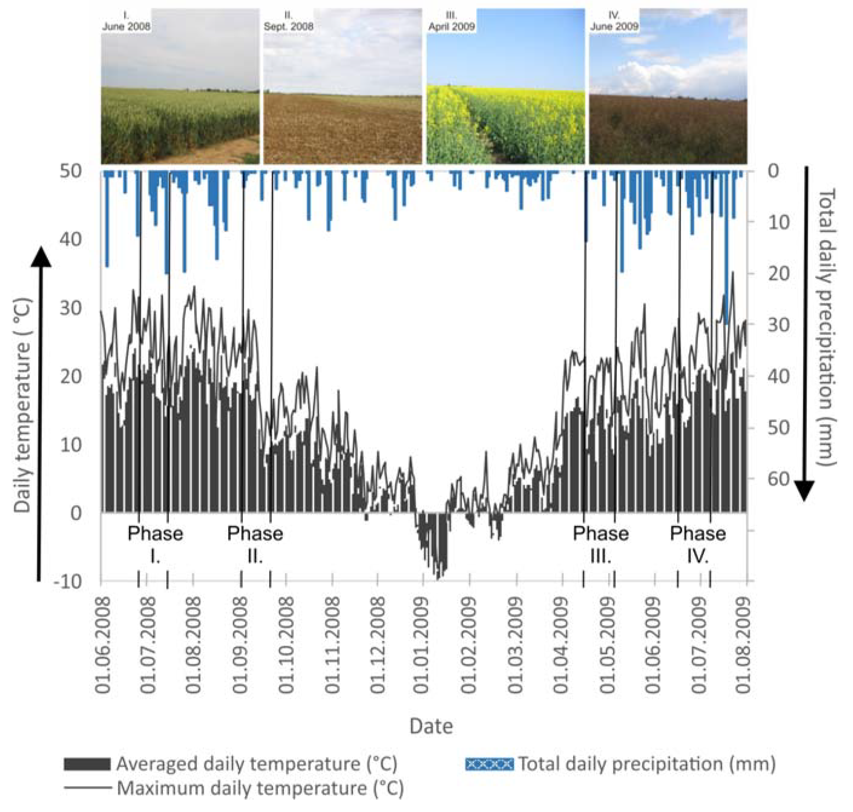
The experimental site is located in the area of Crop Research Institute in Prague, Czech Republic (altitude 345 m a.s.l., 50°5′17.264″ N, 14°17′50.024″ E) with mean annual precipitation 473 mm and mean annual temperature 7.9 °C. The experimental field was established in 1994 and since 1995 three tillage practices have been with the following crop rotation: pea (Pisum sativum)—winter wheat (Triticum aestivum)—oil seed rape (Brassica napus subsp. napus)—winter wheat (Triticum aestivum). The following tillage practices were applied: (i) conventional tillage (CT) with moldboard ploughing up to 22 cm; (ii) reduced tillage (RT) with non-inversion treatment with chisel plough of top 10 cm; and (iii) no-tillage (NT) with application of direct drilling. The soil texture of the experimental field is silty clay loam [37] and the soil was classified as Orthic Luvisol [38]. Basic soil characteristics for the surface layer, namely particle size distribution by Hydrometer method [39], particle density (Water pycnometer method), dry bulk density (four 100 cm3 undisturbed soil samples per each tillage treatment and each experimental phase), organic matter content (total organic carbon content by Walkley–Black procedure [40]) were determined during each experimental phase. Collection of undisturbed soil samples was carried out within the same week as the MDI measurements were performed. Volumetric water contents prior and after the infiltration experiments by employing ThetaProbe ML2x (Delta-T Devices Ltd., UK) were also determined. Own soil specific calibration was carried out in order to obtain high measurement accuracy; determined as ± 1.5 % by vol. The following parameters in the readout unit (HH2 Moisture meter) to display the volumetric water content were set: a0 = 1.859 and a1 = 10.123. The four experimental phases were as follows: (1) June and July 2008 (before harvesting the preceding crop—winter wheat); (2) September 2008 (two weeks after planting the main crop—oil seed rape); (3) April 2009 (the flowering season of the main crop); and (4) June and July 2009 (before harvesting the main crop). The MDI measurements for each experimental phase were performed within one week (5, 7, 6, and 4 days for exp. phase I, II, III, and IV). The HI measurements were lasting longer, only one measurement per day could be managed (almost 1 h of measurement for each applied pressure head, ended by a soil bubbling point). The meteorological data; average and maximum daily temperatures (°C) at 2 m and daily precipitation amounts (mm) is displayed in Figure 1. More detailed evaluation of basic soil characteristics of the top 30 cm together with microbiological analysis and crop yields for the experimental site can be found in a study presented by Mühlbachová et al. [41].
2.2. Devices a Data Analyses Used for Hydraulic Conductivity Determination
2.2.1. Mini Disk Infiltrometer (METER Group, Inc. USA)
Mini Disk infiltrometer (MDI) consists of a single tube divided into two chambers: the lower one serves as water reservoir (95 cm3), which is closed at the bottom with the porous sintered stainless steel disk (0.3 cm thick with diameter of 4.5 cm); and the upper one serves for setting of the pressure head under which the infiltration takes place (from −7 to −0.5 cm). More detailed description of the devices can be found in the User´s manuals [43,44].
The water level drop was recorded manually in regular time intervals between 30 s and 2 min. Three consecutive pressure heads have been applied: −5 cm, −3 cm and −1 cm. The infiltration at each pressure head was allowed for at least 20 min and the infiltration experiment was finished when all water from the reservoir was infiltrated. The measured infiltration data were analyzed based on the steady-state data analysis method proposed by Zhang [45] and recommended in User´s manuals [43,44], fitting the cumulative infiltration data and time with the Philip [46] infiltration equation (Equation (1)):
where C1 (L T−1) and C2 (L T−1/2) are parameters related to hydraulic conductivity and soil sorptivity respectively, I (L) is the cumulative infiltration, and t (T) the time.
The K(h) is than calculated as follows (Equation (2)):
where C1 is the slope of the curve of the cumulative infiltration vs. the square root of time, and A is a value relating the van Genuchten parameters for 12 soil texture classes to the radius of the disk and applied pressure head. The A parameter for the silty clay loam (α = 0.01 and n = 1.23) can be calculated according to the following formula (Equation (3)) or can be taken directly from a table presented in the User´s manual. Corrected and slightly different values were presented in an updated version of the User´s manual in 2014. However, it should be stated that those values of parameter A are derived from the USDA database covering soils from United States [47].
Additionally to that, a detailed study carried out by Dohnal et al. [48] showed that for soils with van Genuchten parameter n < 1.35 the original proposed procedure failed to deliver correct results. The use of the following equation (Equation (4)) is recommended for such soils (with n < 1.35) in order to obtain more reliable K(h) values.
In order to bring the measured data into a wider context, also the well-known computer program Rosetta [49] was used to obtain estimates of Ks together with α and n parameters. The program estimates soil hydraulic parameters with hierarchical pedotransfer functions. In this study, Model 3 (SSCBD) based on percentage content of clay, sand, and silt together with the dry bulk density value was applied. Overview of the used α, n and A parameters for the particular data analysis is presented in Table 1.
Results derived from MDI data by analytical solution presented in MDI Manuals in 2005 and 2014 (with the upgraded equation by Dohnal et al. [48]) were confronted with the inverse solution carried out by means of HYDRUS 2D/3D model [50]. The inverse optimization procedure is based on adjusting the soil hydraulic parameters in order to obtain the best possible agreement between measured and calculated cumulative infiltration data. The inverse solution provides a numerical solution of the Richard´s equation for given initial and boundary conditions, which are specified within the input data. The soil hydraulic functions are commonly described by the expressions of Mualem [51] and van Genuchten [36] (Equations (5) and (6)):
where θE is effective water content (dimensionless), θE = (θ − θr)/(θr − θs), θs (L3L−3) is the volumetric water content at saturation, θr (L3L−3) is the residual volumetric water content, α (L−1) is the dimensionless parameter and m and n are fitting parameters (m = 1−1/n), Kr (h) is the hydraulic conductivity at a certain applied pressure head h (L).
In order to optimize the parameters of Equations (5) and (6), an objective function (Equation (7)) needs to be minimized. The objective function expresses the differences between cumulative infiltration rates determined experimentally for several consecutive pressure heads and cumulative infiltration rates predicted by the model.
where M represents the different sets of measurements such as the cumulative infiltration data or additional information, Nj is the number of measurements in a particular set, Qj*(ti) are the specific measurements at time ti for the jth measurement set, β is the vector of optimized parameters, Qj(ti, β) are the corresponding model predictions for the parameter vector β, vj and wij are weights associated with a particular measurement set or point, respectively. The weighting coefficients vj, are given by Clausnitzer and Hopmans [52], Clausnitzer et al. [53], and Šimůnek et al. [19] as vj = 1/Nj σj2. This defines the objective function as an average weighted squared deviation normalized by measurement variances. If variance of the measurement is not known, vj and wij values are set equal to unity [17]. For all inverse solutions carried out in this study, all vj and wij values were set to be equal to 1.
The axisymetrical vertical flow of water was simulated on a generally described domain with denser structure close to the soil surface (width of 200 cm × depth of 400 cm). The domain was discretized into 85 1D elements, 1111 2D elements with 599 nodes. No hysteresis and no horizontal flow of water has been assumed in the simulation. The initial condition was specified in terms of initial soil water content, expressed as an average value from three measurements. The number of cumulative infiltration data points in the objective function varied between 40 and 80, because each infiltration experiment was unique with its own time intervals between the data records. The following parameters were used in the model in order to optimize parameters α, n and Ks from Equation (6): (i) θs, the saturated soil water content (individually set according to the measured data); (ii) θr, the residual soil water content (in order to avoid fitting to the non-realistic values too close or equal to 0, the parameter was set to the value of 0.08 cm3 cm−3 for all soil treatments and experimental phases); (iii) l, the pore connectivity parameter was also set uniformly to the value of 0.5; (iv) additionally, the values of θfinal (individually set according to the measured data) were also used as input parameters in order to improve the optimization procedure. The boundary conditions were as follows: (i) “Variable head” on the part of the soil surface, where the MDI was located; (ii) “No flux” on the rest of the soil surface and also on the sides of the domain; (iii) “Free drainage” at the bottom of the domain.
2.2.2. Hood Infiltrometer (Umwelt-Geräte-Technik, GmbH., Germany)
The Hood infiltrometer (HI; Umwelt-Geräte-Technik, GmbH., Germany) is an automated device for K(h) and Ks measurement in the field. It consists of a Marriote type water reservoir, circular hood ensuring constant water level and U-tube manometer to control the pressure head. To automate the measurement of infiltrated water, a differential pressure sensor (Honeywell 26 PCA, Honeywell Inc., Charlotte, NC, USA) is used. Measured data are displayed, stored, and transferred to the PC via an UGT micrologger IL-2700.
The infiltration started at pressure head 0 cm (for Ks determination) and then the following pressure heads have been applied: −1 cm, −3 cm, −5 cm (identical with those set by MDI), −7 cm, and −9 cm. If the soil was not bubbling at pressure head smaller than −9 cm, the soil bubbling point was determined at the end of each experiment by increasing the pressure head until a certain moment, when soil started to take air from the soil pores instead of from Mariotte bottle of the HI. The time interval between the data records was set to 30 s. The infiltration time for each applied pressure head was allowed long enough to enable data analysis based on the steady-state infiltration data, between 20 and 60 min. To determine K(h) and Ks from HI data, steady-state data analysis (procedure proposed in the User´s manual [54]), based on the Wooding [14] solution of steady-state infiltration data from a circular source was used (Equation (8)):
where q(h) (L T−1) is steady–state infiltration rate, K(h) (L T−1) is the unsaturated hydraulic conductivity at the applied pressure head (K(h) = Ks exp (αh)), αg (L−1) is the sorptive number (Gardner’s scaling parameter), rd (L) is radius of the disc.
The data analysis procedure described in the User Manual for the HI is using the steady-state infiltration data measured by one disc applying several pressure heads. Parameter α is determined for two neighboring values of steady-state infiltration rates at two neighboring pressure heads (Equation (9)):
Consequently, the hydraulic unsaturated hydraulic conductivities K(hi) and K(hi+1) at the applied pressure heads h are then calculated as follows (Equations (10) and (11)):
2.3. Evaluation of Soil Water Conductive Pore System
Tension or disk infiltrometers (MDI, HI) measurements enable determination of K(h) of the soil matrix by exclusion of pores of certain diameter (macropores) from the infiltration by setting the corresponding water pressure head. Thomas and Phillips discussed the importance and consequences of macropore flow already in 1979 [55]. Luxmoore [56] classified soil pores into three classes; micro-, meso-, and macroporosity. Soil micropores were defined as those pores which drain at soil water pressure head h ≤ −300 cm, mesopores drain at h between −300 cm and −3 cm, and macropores drain at h ≥ −3 cm. According to the capillary rise theory, this indicates that macropores are larger than 0.1 cm in diameter. Macropores, such as interaggregate voids, earthworm channels, shrinkage cracks and root channels, are highly influencing the water flow and thus increasing the risk of leaching contaminants to the groundwater. Watson and Luxmoore [57] found out, that even a small amount of macropores contributes to the total saturated water flux ϕi by 73%. [56]
The number of water conductive pores per unit area Nh was calculated based on Equation (12), while contribution of each soil pores group (macro- and mesopores) to the total saturated water flux ϕi in % was determined based on Equation (13).
where µ (M L−1 T−1) is the dynamic viscosity of water, K(h) in L T−1 is the hydraulic conductivity at the particular pressure head h (L), ρ (M L−3) is the density of water, g (L T−2) is the acceleration due to gravity, π is the dimensionless Ludolph’s number and λh (L) is the representative mean pore radius.
The contribution of macropores and mesopores to the total saturated water flux ϕi (%), can be calculated according to Watson and Luxmoore [57]:
where N is the number of measurements performed in a sequence, h (L) is the corresponding soil water pressure head, K(hi) and K(hi−1) are the hydraulic conductivities (L T−1) obtained for two water pressure heads, and Ks (L T−1) is the saturated hydraulic conductivity.
2.4. Statistical Evaluation
Analysis of variance (ANOVA) on a significance level 0.05 was carried out in order to evaluate differences between the hydraulic conductivity data. ANOVA was also applied on the macro- and mesoporosity data. The Fisher´s least significant difference (LSD) procedure was used to discriminate among the means. Firstly, the Ks and K(h) values were transformed (logarithm to the base of 10) in order to obtain normal distribution of the data. Effects of infiltrometer type and data analysis method have been studied in connection with the space variability (different soil treatment: CT, RT, NT) and time variability (four experimental phases). Amount of variability contributed by the individual factors was evaluated based on Variance component analysis. This procedure is designed to estimate the contribution of multiple factors in a hierarchical manner to the variability of a single dependent variable. Coefficient of variation (CV) has been used to characterize the variations within the particular soil treatment. Statistical software Statgraphics Centurion XV, version 15.2.14 (StatPoint, Inc.) was employed to carry out the statistical evaluation of the data.
3. Results and Discussion
3.1. Basic Soil Characteristics
The soil texture provides an initial indication about the water movement within the soil profile. The particle size distribution curves were determined for the top 10 cm layer in 4 replicates for each soil treatment. No significant differences have been found between the soil treatments showing practically no effect of tillage on particle size distribution data. The soil contained on average 13% of sand (2–0.05 mm), 60% of silt (0.05–0.002 mm), and 21% of clay (<0.002 mm). Averaged values of the soil basic properties (dry bulk density, particle density, porosity and organic matter content expressed as oxidizable carbon Cox) determined for each soil treatment and experimental phase are presented in Table 2. Values of particle density were within the same range during all four experimental phases on all three soil treatments, while the other characteristics were not. A significant loosening effect of soil tillage operations were found in September 2008 for RT and CT plots resulting in lower dry bulk density values and higher values of total porosity. When evaluating the organic matter content, significant differences were found between the treatments; the highest contents were determined for NT plot. The results are in agreement with findings of Çelik et al. [26], who investigated possible differences in physical properties of soils under different tillage treatments for 10 years.
Initial (θinitial) and final (θfinal) soil moisture conditions have been observed during all infiltration experiments. As reported by Matula et al. [58] and Radinja et al. [59], the MDI has shown a high susceptibility to the θinitial for the first applied pressure head. For higher θinitial, significantly smaller K(h) value was recorded, which was in accordance with findings of Zhou et al. [60]. θinitial and θfinal are also essential input data for the HYDRUS 2D/3D software in order to obtain unique solution of the inverse problem. The average θinitial and θfinal values are summarized in Table 3 together with the resulting values of the van Genuchten [36] parameters from Equations (5) and (6) obtained by the inverse solution of the MDI data.
When the α and n parameters are compared to those presented in Table 1, higher values of α were fitted by the HYDRUS 2D/3D while the n parameter level remained unchanged. The quality of the fit was evaluated on the basis of R2 coefficient, and by graphical comparison of the measured and fitted data; both were showing very good agreement between the measured and fitted data for all infiltration experiments and all applied pressure heads.
3.2. Unsaturated Hydraulic Conductivity K(h)
The K(h) values were determined on the basis of MDI measurements for pressure heads of −5, −3, and −1 cm and on the basis of the HI measurements for pressure heads of −1, −3, −5, −7 and if the soil was not bubbling also −9 cm (in September 2008, when some effect of soil tillage treatment has been expected, also pressure head of −0.5 was applied during the measurements). Relatively high natural variability within the soil treatments was expressed in relatively high values of coefficient of variation (CV). Comparison of the resulting K(h) data together with CVs within the particular soil treatments determined on the basis of HI and MDI measurements is displayed in Figure 2. The MDI data in Figure 2 were analyzed according to the most up to date analysis suggested in the Manual, method of Dohnal et al. [48].
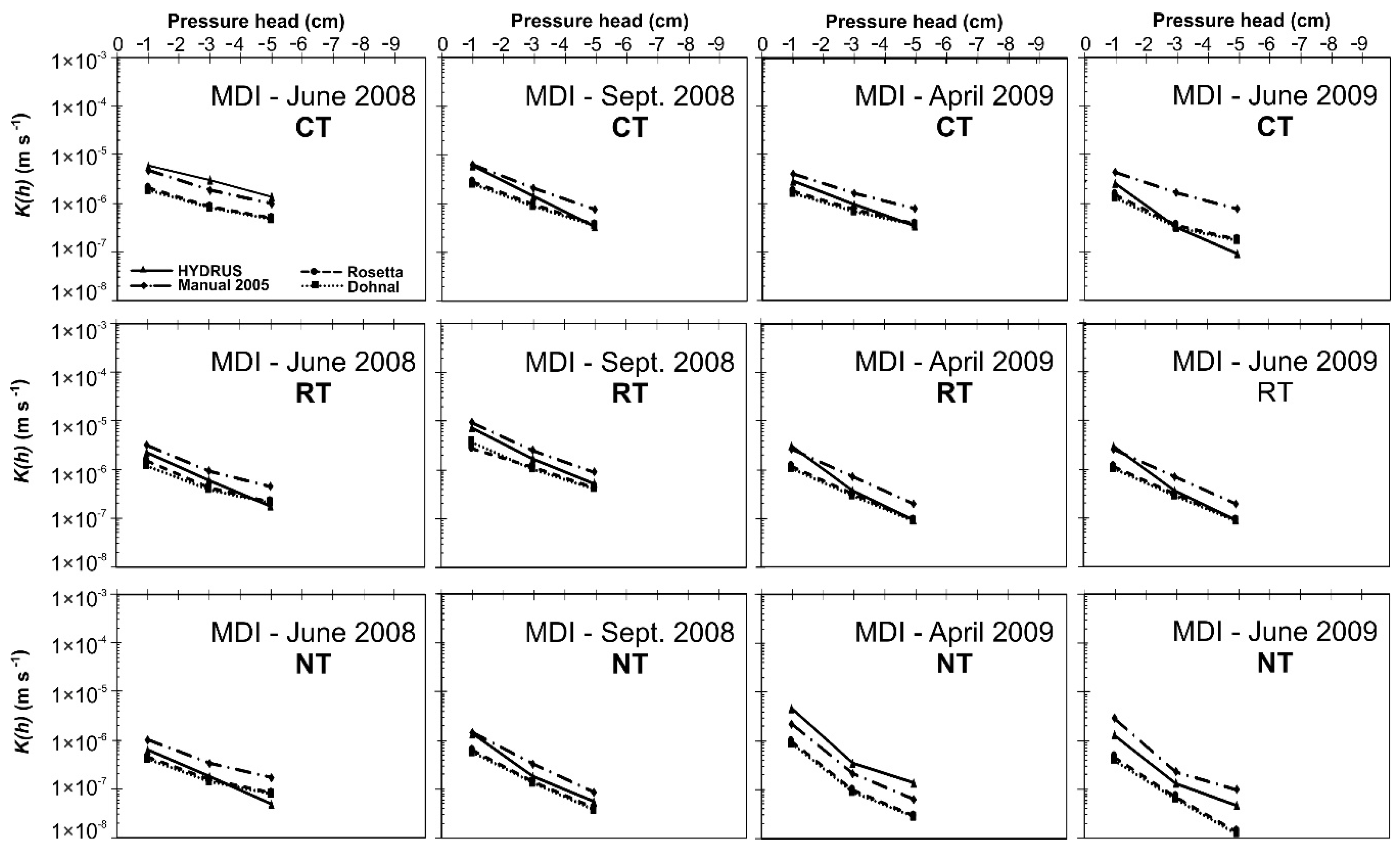
Log transformed K(h) data from HI and MDI were analyzed and compared. Although the K(h) experiments by HI were measured up to the soil bubbling point, only the K(h) for the same pressure heads as for the MDI were used in the statistical evaluation (−5, −3, and −1 cm). Considering two types of steady-state data analyses using different α and n parameters as described in section “Materials and Methods” and one transient data analysis, a total number of 324 logK(h) for MDI and 108 logK(h) for HI was evaluated. The effect of the applied data analysis can be seen on an overview picture comparing the averaged K(h) MDI data obtained by the four types of data analysis for each soil treatment and experimental phase (Figure 3). Clear differences have been observed, especially the HYDRUS and Manual 2005 data analyses were showing higher K(h) values which were determined as statistically significant.
The statistical evaluation of the data has started with identification of the factors affecting the K(h) results and thus explaining the variability of the determined logK(h) values (Table 4). The following factors in this order have been evaluated by variance component analysis: (i) type of the infiltrometer incl. type od the data analysis, (ii) applied pressure head, (iii) soil treatment, and (iv) experimental phase. The factor contributing the most was the soil treatment explaining 29% of the total variability. Almost the same level of contribution was determined for the infiltrometer type and data analysis method; 28%. Applied pressure head explained 23% of the total variability, while the time factor (experimental phase) contributed only by 12% and only 8% of total variability remained unexplained by random factors. All tested factors have shown their significance in further statistical analysis of variance.
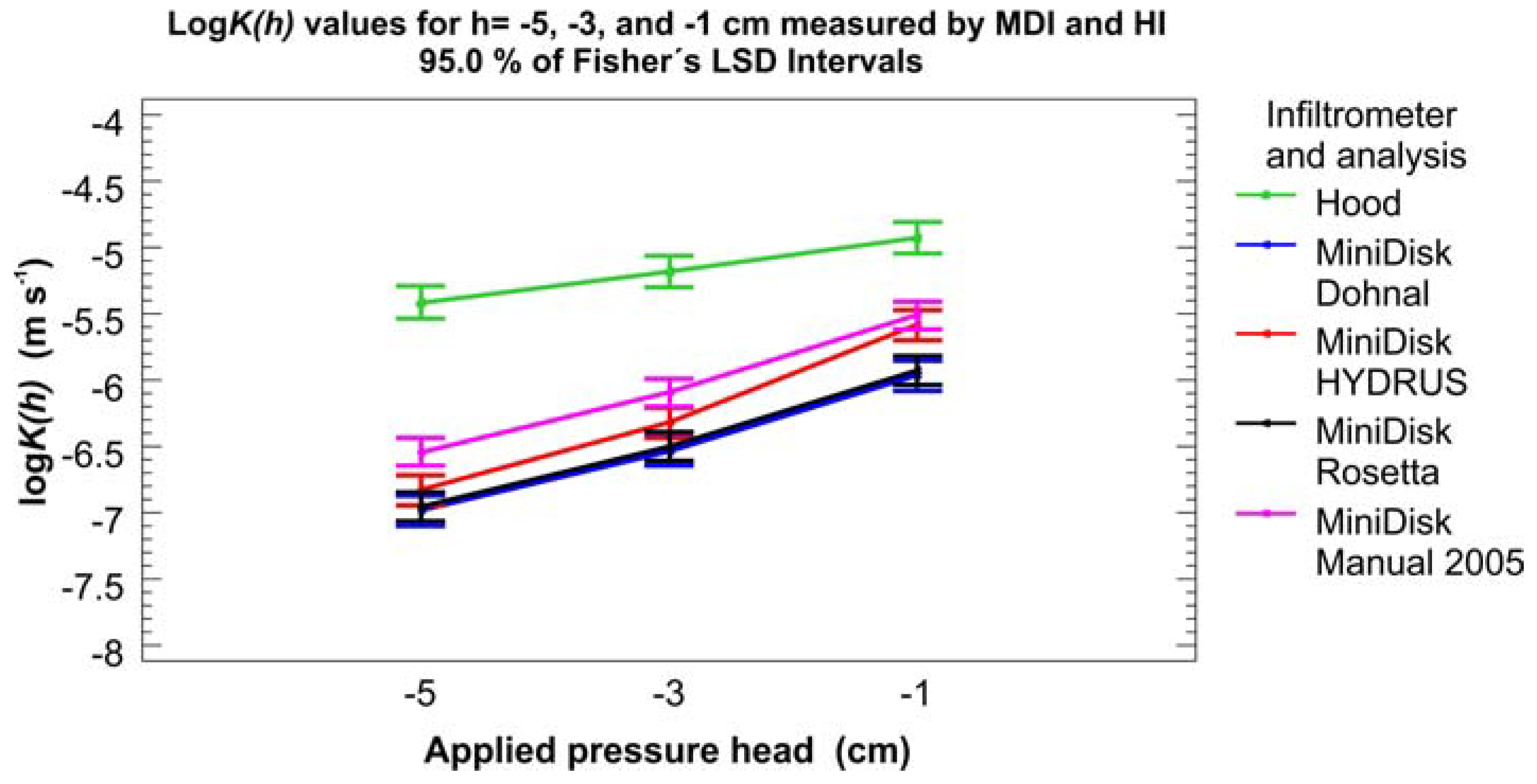
Significantly higher logK(h) values were determined by HI (Figure 4). Statistically significant differences have been observed between the logK(h) values determined on CT, RT and NT plots, that is why only data from NT were used in further analyses in order to evaluate the effect the infiltrometer type. When higher values of logK(h) determined for RT and CT plots were removed from the source data, a certain shift of data along the y axis on Figure 5 when compared to Figure 4 was observed. However, the order and shapes of the logK(h) curves remained very similar. Three homogeneous groups were identified: (i) the lowest values were determined by MDI with application of Dohnal´s and Rosetta analyses; (ii) higher values were determined by MDI with application of numerical analysis by HYDRUS and original analysis presented in Manual 2005; (iii) the highest values were determined by HI. When evaluating the LSD into more details in Figure 4 and 5, a different situation at pressure head −1 cm can be observed when only data from NT were evaluated. Pressure head of −1 cm is close to saturation and the numerical model HYDRUS has tried to match the recorded higher infiltration rates. The analytical solution originally presented in Manual 2005 has been proven to provide inaccurate estimates of K(h) values for soils with n < 1.35.
Schwärzel and Punzel [61] in their detailed study presented a comparison of the HI performance to disk infiltrometer measurements. They observed and discussed significantly higher values of K(h) measured by HI on a sandy loam soil in comparison with disk infiltrometer (placed on a contact material). The difference was around one order of magnitude, which is similar to the differences observed in this study on a silty clay loam soil (without any use of a contact material). The effect of the contact layer was concluded by Schwärzel and Punzel [61] as negligible when compared with the observed differences between the HI and disk infiltrometer results. They have also stated that the preparation of the soil surface for disk infiltrometer measurements can lead to the sealing and smearing of the pores of the soil surface and thus decreasing the infiltration rate from the disk infiltrometers especially close to saturation. Some differences between the resulting K(h) values obtained by MDI and HI can be also caused by an effect of the initial soil moisture content [58]. The differences between the designs of the infiltrometers, providing different size of the infiltration area and different approach to the contact between the infiltrometer and soil surface, together with different order of applied pressure heads are probably the main reasons causing different results. Most of the currently used tension infiltrometers including the MDI consist of a base with semi-permeable membrane, which allows water to infiltrate into the soil under a set pressure head. Good contact between the membrane and the infiltration surface is critically important for the correct measurement. In order to ensure the good contact, a thin layer of a contact material is usually recommended in the User manuals. Some possible effects of the contact material use in tension infiltrometry, such as discrepancy between the pressure head applied on the contact material and soil surface, changes of the natural contact material during the infiltration process due to a fine particles movement, were researched and discussed [62,63]. HI does not require any contact material, since water is applied directly on the soil surface, this might contribute to differences between MDI and HI results. Special care should be taken when the K(h) data are recorded and compared to each other, because only data originating from the same infiltrometer type and applied data analysis can be compared without an additional source of error. In a practical point of view, different databases of soil hydraulic properties contain certain amount of K(h) and Ks data. Not much is usually clarified about the device and data analysis method used for its determination.
3.3. Saturated Hydraulic Conductivity Ks
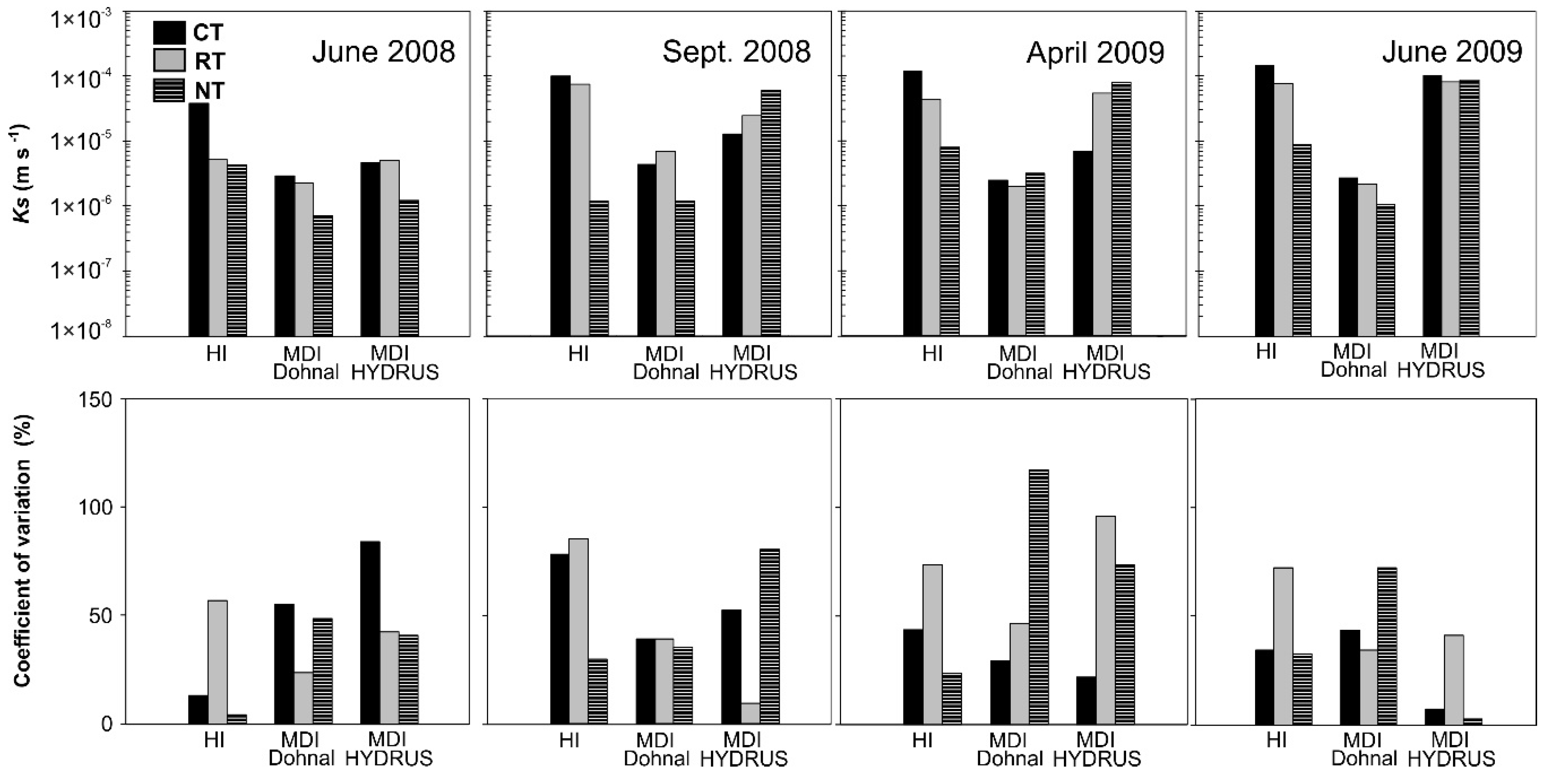
The Ks was directly measured by the HI; pressure head during the experiments was set to 0 cm. The Ks from MDI was estimated by extrapolation based on the logK(h) data distribution and also by inverse solution in HYDRUS 2D/3D. Inverse parametrization is a quite common technique applied on near-saturated tension infiltrometer (MDI) data [19,64]. Schwen et al. [65] recommended careful extrapolation of the near-saturated data with emphasis on possible over-extrapolation too far beyond the measured range. The overview of the Ks data determined by MDI and HI is displayed in the upper part of Figure 6. The Ks measured by HI were previously compared with data originating from Pressure infiltrometer by Matula and Kozáková [66], device constructed for Ks measurement in-situ. No significant differences have been found between the Ks data measured by Pressure infiltrometer and HI, regardless of the soil treatment and experimental phase. Thus, the Ks from HI were taken as a reference for data estimated on the basis of MDI data.
With respect to the soil treatment, the Ks values were in the following order during all four experimental phases CT > RT > NT. The Ks determined on the basis of the MDI infiltration experiments were significantly lower than those measured by HI. Generally, the Ks data obtained by the inverse solution in HYDRUS 2D/3D were higher for all four experimental phases. This can be explained by the effect of macropores starting to be active close to saturation accompanying by a large increase in amount of infiltrated water per unit of time, which the software tried to match. Relatively high variation of Ks data was observed (lower part of Figure 6). When evaluating the CV in terms of type of the infiltrometer, similar values were observed for Ks data: 46% for HI, 49% for MDI-Dohnal and 46% for MDI-HYDRUS. The CV values were not showing any trend supporting the high importance of spot selection for the field infiltration experiment. This is documented by some randomly high CV values during each experimental phase observed by different infiltrometers on different soil treatment types; values of CV higher than 100%. That is why more replicates on a carefully taken spots should be taken in order to obtain representative values with smaller CV.
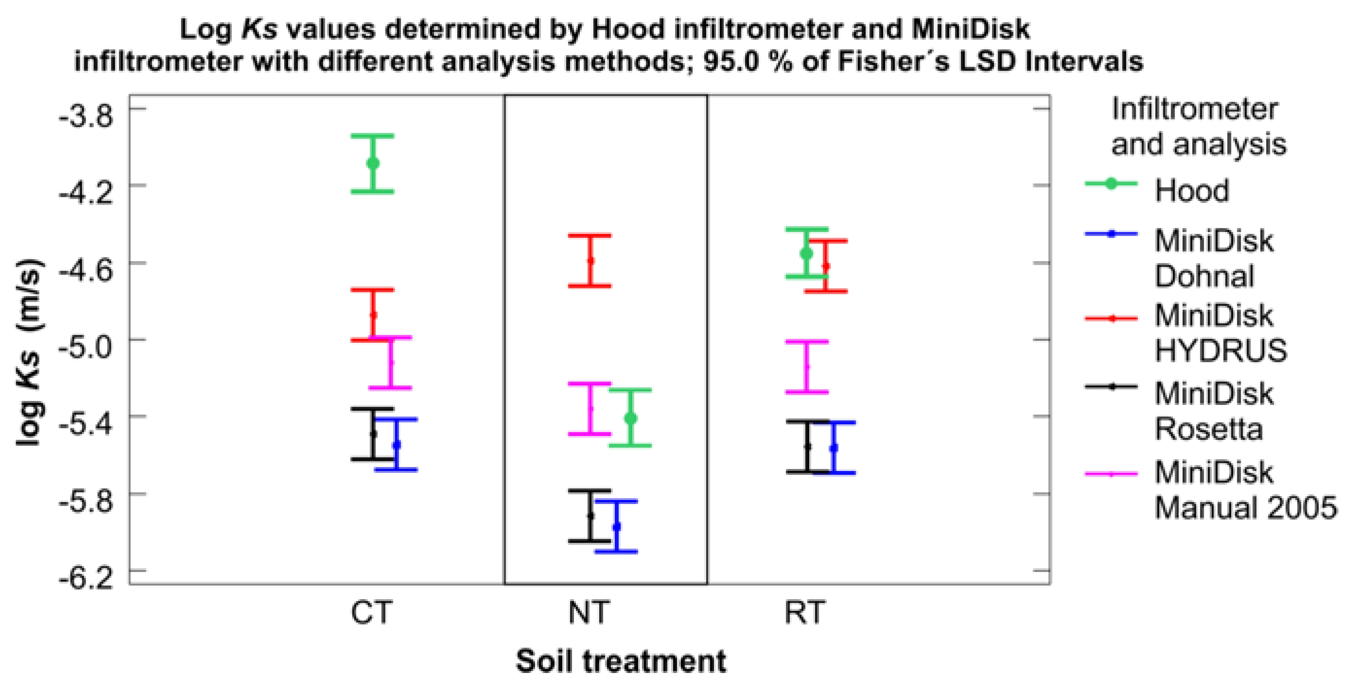
Significantly lower values systematically underestimating the logKs values on all three tillage treatments determined by MDI based on extrapolation of the Dohnal et al. [48] data are displayed in Figure 7.
The significant effect of the data analysis used for the MDI data evaluation is clearly seen on Figure 7. The estimates obtained by HYDRUS 2D/3D modelling were the highest on all soil treatments, while the results obtained by the method of Dohnal et al. [48] and on the basis of estimates of parameters α and n by Rosetta showed almost no difference suggesting the proper approach to the MDI data. HYDRUS 2D/3D in its simple settings probably overestimated the Ks values in spite of very high values of R2 between the measured and fitted infiltration data. Requirements for inverse modelling of soil hydraulic properties has been discussed by Hopmans and Simunek [67] and Kumar et al. [3] who pointed out the amount of measured variables, boundary condition setting, errors in the measured variable and type of the soil as factors affecting the inverse solution. Also Zou et al. [68] attributed the ill-posedness of the inverse problem to the high nonlinearity of the data in unsaturated flow problems. Kumar et al. [3] reported the Ks values obtained in the laboratory one order of magnitude higher than those obtained in the field and also highlighted importance of results from the laboratory as input data for the inverse modelling of the field data. More detailed study regarding the HYDRUS 2D data analysis settings would be required. Only one hydraulic model; van Genuchten [36] – Mualem [51] was used in this study. Further options are offered in the HYDRUS 2D software; e.g., Kosugi [69] log-normal model, or Durner [70] dual porosity model. The dual porosity model especially could be beneficial, because as shown further, the contribution of macropores to the total saturated flux is very significant. Significant effect of data analysis selection on resulting K(h) and Ks results are also reported by Fatehnia et al. [71].
When evaluating the Ks and K(h) measurements, the representativeness of the experimental area and the spot selection for the infiltrometer placement are crucial. With increasing infiltration area given by the dimensions of the infiltrometer base, the increasing representativeness and more stable Ks data were reported by Lai et al. [72] who studied the size dependency of Ks using double-ring infiltrometer. The recommended ring diameter was bigger than 80 cm in order to quantify the Ks reliably. However, practically no other infiltrometer type, except the double ring, has such a large diameter of the infiltration area. Naturally, an increased number of replicated measurements can lead to more reliable results. Picciafuoco et al. [73] based on the selected width of 95% confidence interval and area size, determined a number of replicates needed for reliable results. A minimum number of 5 replicates was reported for a 110 m2 area in order to obtain an accuracy level as suggested by Ahmed et al. [74]. Rienzner and Gandolfi [75] compared Ks values obtained by Guelph permeameter and by tension infiltrometer concluding that the Ks values obtained by tension infiltrometer are systematically lower, which is in agreement with our study where the Ks values obtained by MDI were compared to HI. However, much smaller variability in both, space and time for the tension infiltrometers has been observed when compared to our study. Reynolds et al. [76] compared the Ks values obtained by tension infiltrometer, pressure infiltrometer and soil core determination in the laboratory with the following results: (i) different methods yielded different Ks values; (ii) tension infiltrometer provided comparable results to other methods only for Ks values smaller than 10−4 m s−1; (iii) the tension infiltrometer yielded the smallest CV for the cracking clay loam; (iv) the soil core laboratory method performed well on structure less sand and structured loam soil, however in the cracking clay it yielded high CV values; and (v) the pressure infiltrometer provided comparable results to the other methods. Only for the cracking clay loam soil it yielded in a large range of the Ks data accompanied by high CV. Laboratory comparison of field infiltrometers, namely double ring infiltrometer, Philip-Dunne infiltrometer and Mini Disk infiltrometer, on artificially prepared sandy profiles in three 208 dm3 barrels, was studied by Nestingen et al. [77]. Very low CV values were determined, in average 9.1% for the Double Ring infiltrometer, 13.7% for the Philip-Dune infiltrometer and 22.7% for the Mini Disk infiltrometer. The CV values determined for Ks values in our study ranged in average between 22% (HI on NT plot) and 72% (HI on RT plot). Although the CV values are higher than those reported by Nestingen et al. [77], they are lower than values presented in studies of Ahmed et al. [74] and Olson et al. [78] reporting the averaged CV values of 168% and 91%, respectively.
An increasing number of studies is dealing with the comparison of different techniques to determine K(h) and Ks data e.g., Reynolds et al. [76] and Lai et al. [72] or more recent studies by Morbidelli et al. [79], Nestingen et al. [77] and Ghosh et al. [80] are showing the importance of these characteristics. This poses an increasing need of some benchmark or reference method to determine them and consequently relate already existing data in order to obtain comparable and reliable data.
3.4. Mesopore and Macropore Contributions to the Total Saturated Flux
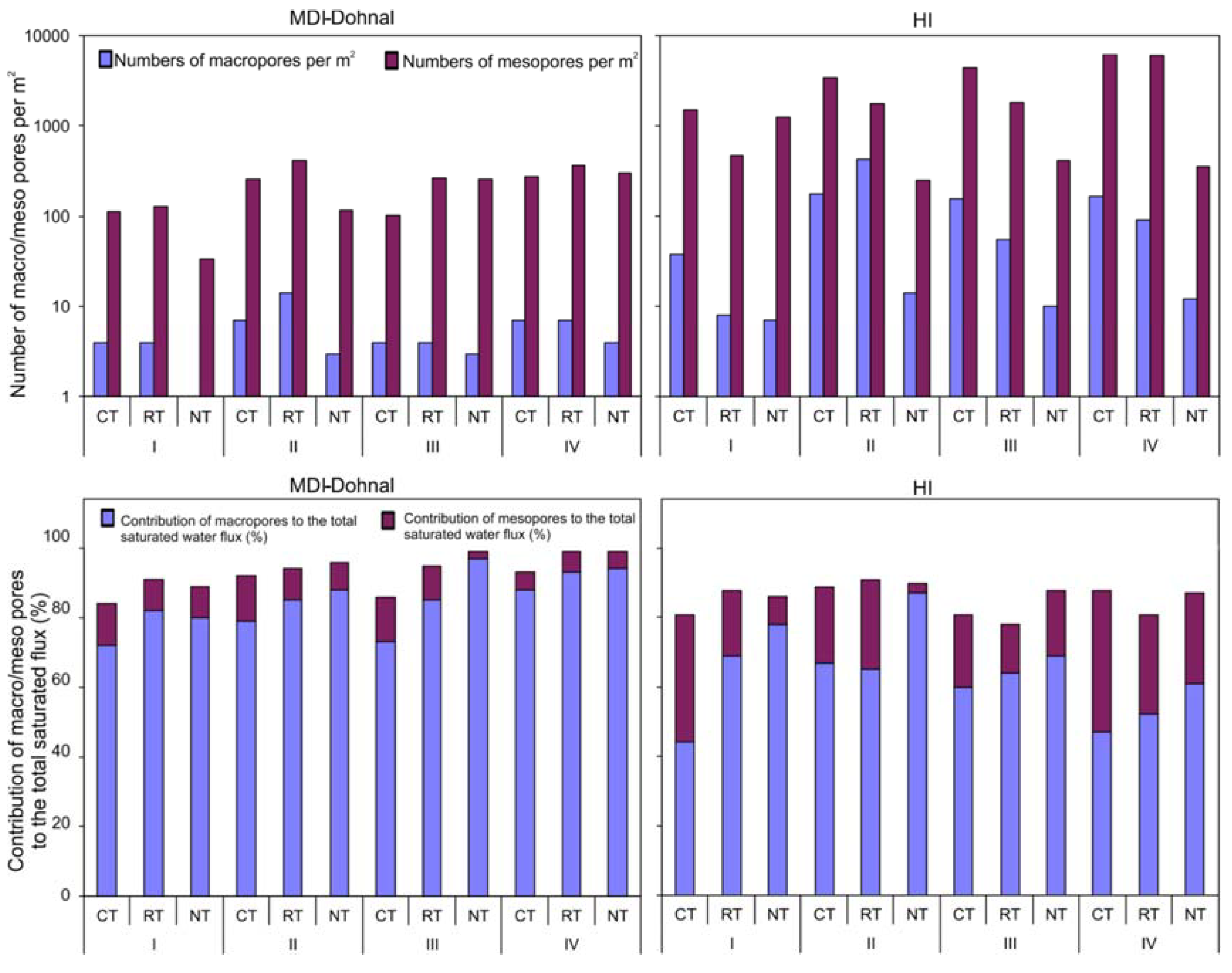
On average, the number of mesopores was approximately 12-times higher than the number of macropores. There were about two times more macropores determined by HI than by MDI; however, the difference was not statistically significant. That is probably due to a large increase in number of macropores determined for the second experimental phase (after tillage operation in September 2008), when the number was reaching its maximum: 417/m2 determined by MDI and 1212/m2 by HI. On the other hand, there was about 1.5 times more mesopores determined by HI compared to the numbers determined by MDI. In spite of a smaller amount of macropores, their contribution to the total saturated water flux was in average 76%. Numbers of mesopores and macropores with their averaged contributions to the total saturated flux in % for each tillage treatment and each experimental phase are displayed in Figure 8. Based on the results, it can be seen that such a small device as the MDI can successfully quantify the macropore contribution to the water transport through the soil profile.
Although the values determined based on the MDI and HI differ, it is clear from Figure 8 that the macropores are crucial in water infiltration regardless of their number or tillage treatment. Importance of macropores as preferential pathways for flow of water is highlighted also by other studies; e.g., Sauer et al. [27], Angulo-Jaramillo et al. [81], Cameira et al. [29], Moret and Arrúe [30]. All of the authors agreed that the water flow in soils is mainly conducted by macropores even though they represent only a small fraction of the total porosity.
4. Conclusions
Relatively large K(h) and Ks dataset was collected during this study. Performance comparison of MDI and HI was carried out for a silty clay loam soil under three different soil treatments (CT, RT, and NT) during four experimental phases reflecting seasonal changes in a cultivated field. In spite of its small size, the MDI performed very well. MDI based K(h) data were responding to changes in soil structure due to tillage operations showing a significant soil loosening effect originating from tillage operations performed just before the 2nd experimental phase. Based on the MDI infiltration data, number of macrospores and their contribution to the total saturated flux was successfully determined. That is especially important for possible simulations of contaminant transport through the soil profile.
The steady-state data analysis method based on hydraulic input parameters originating from different sources resulted in different K(h) values. More importantly, significantly higher K(h) values were determined by the method described in MDI User’s manual from 2005 than from 2014 where the n parameter correction was implemented. Based on our findings, the K(h) data of fine-textured and structural soils evaluated without the correction by Dohnal et al. [48] are consistently almost one order of magnitude higher. This finding should be addressed in utilization of older MDI data for comparative studies and their use from hydraulic properties databases.
Results based on HI measurements were showing the same trends, higher values of K(h) and Ks for CT and RT plots when compared to NT. However, the particular K(h) values were higher than those determined by MDI. Similarly, a higher number of macropores and mesopores was calculated based on HI data. Estimates of Ks values on the basis of MDI data (regardless of the data analysis) in the present study are too divergent from the measured values by HI, and thus this approach to Ks determination cannot be generally recommended.
The following evaluation table (Table 5) can be helpful in selection of K(h) and Ks determination method.
Author Contributions
K.B. and S.M. conceptualized the research problem and formulated aims and objectives of the study; K.B. and M.M. performed field and laboratory experimental work; K.B. evaluated the measured data; all authors contributed to the results interpretation, manuscript writing and revision. All authors have read and agreed to the published version of the manuscript.
Funding
This study was financially supported by NATIONAL AGENCY FOR AGRICULTURAL RESEARCH (NAZV) of the Ministry of Agriculture of the Czech Republic, grant number QK1720285.
Acknowledgments
Special thanks belong to Růžek and Mühlbachová from the Crop Research Institute in Prague, who are managing the experimental field and enabled this research to be carried out.
Conflicts of Interest
The authors declare no conflict of interest.
References
- Shouse, P.J.; Mohanty, B.P. Scaling of near-saturated hydraulic conductivity measured using disc infiltrometers. Water Resour. Res. 1998, 34, 1195–1205. [Google Scholar] [CrossRef]
- Buczko, U.; Bens, O.; Hüttl, R.F. Tillage effects on hydraulic properties and macroporosity in silty and sandy soils. Soil Sci. Soc. Am. J. 2006, 70, 1998–2007. [Google Scholar] [CrossRef]
- Kumar, S.; Sekhar, M.; Reddy, D.V.; Mohan Kumar, M.S. Estimation of soil hydraulic properties and their uncertainty: Comparison between laboratory and field experiment. Hydrol. Process. 2010, 24, 3426–3435. [Google Scholar] [CrossRef]
- Standard Test Method for Infiltration Rate of Soils in Field Using Double-Ring Infiltrometer; ASTM D3385–03; ASTM International: West Conshohocken, PA, USA, 2003. [CrossRef]
- Standard Test Methods for Measurement of Hydraulic Conductivity of Unsaturated Soils; ASTM D7664–10e1; ASTM International: West Conshohocken, PA, USA, 2010. [CrossRef]
- Geotechnický Průzkum a Zkoušení—Laboratorní Zkoušky Zemin—Část 11: Stanovení Propustnosti; ČSN EN ISO 17892–11 (721007); Český Normalizační Institut: Prague, Czech Republic, 2019.
- Reynolds, W.D.; Topp, G.C. Soil Water Analyses. In Soil Sampling and Methods of Analysis, 2nd ed.; Carter, M.R., Gregorich, E.G., Eds.; CRC Press: Boca Raton, FL, USA, 2007; pp. 918–936. [Google Scholar]
- Casey, F.X.M.; Derby, N.E. Improved design for an automated tension infiltrometer. Soil Sci. Soc. Am. J. 2002, 66, 64–67. [Google Scholar] [CrossRef]
- Madsen, M.; Chandler, D. Automation and use of mini disk infiltrometers. Soil. Sci. Soc. Am. J. 2007, 71, 1469–1472. [Google Scholar] [CrossRef]
- Rodný, M.; Rodný, P.; Šurda, P.; Matula, S.; Miháliková, M.; Chala, A. Automation of mini disk infiltrometer based on particle tracking principle. Acta Hydrol. Slovaca 2013, 14, 460–465. [Google Scholar]
- Šurda, P.; Rodný, M.; Nagy, V.; Matula, S.; Miháliková, M.; Chala, A. Spatial variability of the hydraulic conductivity of the soil with biological soil crust in the horizontal and vertical direction. Acta Hydrol. Slovaca 2013, 14, 466–472. [Google Scholar]
- Kameníčková, I.; Larišová, L.; Stoklásková, A. The impact of different tillage treatments on hydraulic conductivity of loamy soil. Acta Universitatis Agriculturae Silviculturae Mendelianae Brunensis 2012, 5, 109–114. [Google Scholar] [CrossRef] [Green Version]
- Angulo-Jaramillo, R.; Vandervaere, J.-P.; Roulier, S.; Thony, J.-L.; Gaudet, J.-P.; Vauclin, M. Field measurement of soil surface hydraulic properties by disc and ring infiltrometers. A review and recent developments. Soil Till. Res. 2000, 55, 1–29. [Google Scholar] [CrossRef]
- Wooding, R.A. Steady infiltration from a shallow circular pond. Water Resour. Res. 1968, 4, 1259–1273. [Google Scholar] [CrossRef]
- White, I.; Sully, M.J. Macroscopic and microscopic capillary length and time scales from field infiltration. Water. Resour. Res. 1987, 23, 1514–1522. [Google Scholar] [CrossRef]
- Reynolds, W.D.; Elrick, D.E. Determination of hydraulic conductivity using a tension infiltrometer. Soil Sci. Soc. Am. J. 1991, 55, 633–639. [Google Scholar] [CrossRef]
- Ventrella, D.; Losavio, N.; Vonella, A.V.; Leij, F.J. Estimating hydraulic conductivity of a fine-textured soil using tension infiltrometry. Geoderma 2005, 124, 267–277. [Google Scholar] [CrossRef]
- Lazarovitch, N.; Ben-Gal, A.; Šimůnek, J.; Shani, U. Uniqueness of soil hydraulic parameters determined by a combined Wooding inverse approach. Soil Sci. Soc. Am. J. 2007, 71, 860–865. [Google Scholar] [CrossRef] [Green Version]
- Šimůnek, J.; Angulo-Jaramillo, R.; Shaap, M.G.; Vandervaere, J.P.; van Genuchten, M.T. Using an inverse method to estimate the hydraulic properties of crusted soils from tension-disc infiltrometer data. Geoderma 1998, 86, 61–81. [Google Scholar] [CrossRef]
- Šimůnek, J.; van Genuchten, M.T. Estimating unsaturated soil hydraulic properties from tension disc infiltrometer data by numerical inversion. Water Resour. Res. 1996, 32, 2683–2696. [Google Scholar] [CrossRef]
- Šimůnek, J.; van Genuchten, M.T. Estimating unsaturated soil hydraulic properties from multiple tension disc infiltrometer data. Soil Sci. 1997, 162, 383–398. [Google Scholar] [CrossRef]
- Strudley, M.W.; Green, T.R.; Ascough Ii, J.C. Tillage effects on soil hydraulic properties in space and time: State of the science. Soil Till. Res. 2008, 99, 4–48. [Google Scholar] [CrossRef]
- Rasiah, V.; Kay, B.D. Runoff and soil loss as influenced by selected stability parameters and cropping and tillage practices. Geoderma 1995, 68, 321–329. [Google Scholar] [CrossRef]
- Price, K.; Jackson, C.R.; Parker, A.J. Variation of surficial soil hydraulic properties across land uses in the southern Blue Ridge mountains, North Carolina, USA. J. Hydrol. 2010, 383, 256–268. [Google Scholar] [CrossRef]
- Friedrich, T. Engineering for conservation agriculture—Trends, concepts and challenges in a global perspective. In Proceedings of the International Soil Tillage Research Organisation Conference, Brisbane, Australia, 13–18 July 2003. [Google Scholar]
- Çelik, İ.; Günal, H.; Acar, M.; Acir, N.; Bereket Barut, Z.; Budak, M. Strategic tillage may sustain the benefits of long-term no-till in a Vertisol under Mediterranean climate. Soil Till. Res. 2019, 185, 17–28. [Google Scholar] [CrossRef]
- Sauer, T.; Clothier, B.E.; Daniel, T.C. Surface measurements of the hydraulic properties of a tilled and untilled soil. Soil Till. Res. 1990, 15, 359–369. [Google Scholar] [CrossRef]
- Ankeny, M.D.; Kaspar, T.C.; Horton, R. Characterization of tillage and traffic effects on unconfined infiltration measurement. Soil Sci. Soc. Am. J. 1990, 54, 810–837. [Google Scholar] [CrossRef] [Green Version]
- Cameira, M.R.; Fernando, R.M.; Pereira, L.S. Soil macropore dynamics affected by tillage and irrigation for a silty loam alluvial soil in southern Portugal. Soil Till. Res. 2003, 70, 131–140. [Google Scholar] [CrossRef]
- Moret, D.; Arrúe, J.L. Characterizing soil water-conducting macro and mesoporosity as influenced by tillage using tension infiltrometry. Soil Sci. Soc. Am. J. 2007, 71, 500–506. [Google Scholar] [CrossRef] [Green Version]
- Cassel, D.K. Spatial and temporal variability of soil physical properties following tillage of Norfolk loamy sand. Soil Sci. Soc. Am. J. 1983, 47, 196–201. [Google Scholar] [CrossRef]
- Mapa, R.B.; Green, R.E.; Santo, L. Temporal variability of soil hydraulic-properties with wetting and drying subsequent to tillage. Soil Sci. Soc. Am. J. 1986, 50, 1133–1138. [Google Scholar] [CrossRef]
- Rousseva, S.S.; Ahuja, L.R.; Heathman, G.C. Use of a surface gamma-neutron gauge for in-situ measurement of changes in bulk density of the tilled zone. Soil Till. Res. 1988, 12, 235–251. [Google Scholar] [CrossRef]
- Moret, D.; Arrúe, J.L. Dynamics of soil hydraulic properties during fallow as affected by tillage. Soil Till. Res. 2007, 96, 103–113. [Google Scholar]
- Kreiselmeier, J.; Chandrasekhar, P.; Weninger, T.; Schwen, A.; Julich, S.; Feger, K.-H.; Schwärzel, K. Temporal variations of the hydraulic conductivity characteristic under conventional and conservation tillage. Geoderma 2020, 362, 114127. [Google Scholar] [CrossRef]
- Van Genuchten, M.T. A closed-form equation for predicting the hydraulic conductivity of unsaturated soils. Soil Sci. Soc. Am. J. 1980, 44, 892–898. [Google Scholar] [CrossRef] [Green Version]
- Soil Survey Staff. Keys to Soil Taxonomy, 12th ed.; USDA-Natural Resources Conservation Service: Washington, DC, USA, 2014; p. 360.
- IUSS Working Group WRB. World Reference Base for Soil Resources 2014, update 2015. In International Soil Classification System for Naming Soils and Creating Legends for Soil Maps; World Soil Resources Reports No. 106; FAO: Rome, Italy, 2015; p. 192. [Google Scholar]
- Geotechnický Průzkum a Zkoušení—Laboratorní Zkoušky Zemin—Část 4: Stanovení Zrnitosti; ČSN EN ISO 17892–4 (721007); Český Normalizační Institut: Prague, Czech Republic, 2017.
- Walkley, A.; Black, I.A. An examination of the Degtjareff method for determining organic carbon in soils: Effect of variations in digestions and of inorganic soil constituents. Soil Sci. 1934, 63, 251–263. [Google Scholar] [CrossRef]
- Mühlbachová, G.; Kusá, H.; Růžek, P. Soil characteristics and crop yields under different tillage techniques. Plant Soil Environ. 2015, 61, 566–572. [Google Scholar] [CrossRef] [Green Version]
- Agrometeorological database. Available online: https://www.vurv.cz/meteo/ (accessed on 14 December 2018).
- Decagon Devices; METER Group. Mini Disk Infiltrometer—User’s Manual, 3rd version; Decagon Devices, Inc.: Pullman, WA, USA, 2005; p. 18. [Google Scholar]
- Decagon Devices; METER Group. Mini Disk Infiltrometer—User’s Manual; Version: September 10/2014; Decagon Devices, Inc.: Pullman, WA, USA, 2014; p. 21. [Google Scholar]
- Zhang, R. Infiltration models for the disk infiltrometer. Soil Sci. Soc. Am. J. 1997, 61, 1597–1603. [Google Scholar] [CrossRef]
- Philip, J.R. The theory of infiltration: 4. Sorptivity and algebraic infiltration equations. Soil Sci. 1957, 84, 257–264. [Google Scholar] [CrossRef]
- Rawls, W.J.; Brakensiek, D.L.; Saxton, K.E. Estimation of soil water properties. Trans. ASAE 1982, 25, 1316–1320. [Google Scholar] [CrossRef]
- Dohnal, M.; Dušek, J.; Vogel, T. Improving hydraulic conductivity estimates from Minidisk infiltrometer measurements for soils with wide pore-size distributions. Soil Sci. Soc. Am. J. 2010, 74, 804–811. [Google Scholar] [CrossRef]
- Schaap, M.G.; Leij, F.J.; van Genuchten, M.T. ROSETTA: A computer program for estimating soil hydraulic parameters with hierarchical pedotransfer functions. J. Hydrol. 2001, 251, 163–176. [Google Scholar] [CrossRef]
- Šimůnek, J.; Šejna, M.; van Genuchten, M.T. The HYDRUS-2D software package for simulating the two-dimensional movement of water, heat, and multiple solutes in variably-saturated media. In Version 2.0. USA Salinity Laboratory; Agricultural Research Service, USA Department of Agriculture: Riverside, CA, USA, 1999. [Google Scholar]
- Mualem, Y. A new model for predicting the hydraulic conductivity of unsaturated porous media. Water Resour. Res. 1976, 12, 513–522. [Google Scholar] [CrossRef] [Green Version]
- Clausnitzer, V.; Hopmans, J.W. Non-linear parameter estimation: LM_OPT. General-purpose optimization code based on the Levenberg-Marquart algorithm. In Land, Air and Water Resources; Paper No. 100032; University of California: Davis, CA, USA, 1995. [Google Scholar]
- Clausnitzer, V.; Hopmans, J.W.; Starr, J.L. Parameter uncertainty analysis of common infiltration models. Soil Sci. Soc. Am. J. 1998, 60, 1477–1487. [Google Scholar] [CrossRef] [Green Version]
- Umwelt-Geräte-Technik. Operating Instructions for Hood Infiltrometer IL-2700; Umwelt Geräte Technik GmbH: Münchenberg, Germany, 2005; p. 32. [Google Scholar]
- Thomas, G.W.; Philips, R.E. Consequences of water movement in macropores. J. Environ. Qual. 1979, 8, 149–156. [Google Scholar] [CrossRef]
- Luxmoore, R.J. Micro-, meso-, and macroporosity of soil. Soil Sci. Soc. Am. J. 1981, 45, 671–672. [Google Scholar] [CrossRef]
- Watson, K.W.; Luxmore, R.J. Estimating macroporosity in a forest watershed by the use of a tension infiltrometer. Soil Sci. Soc. Am. J. 1986, 50, 578–582. [Google Scholar] [CrossRef]
- Matula, S.; Miháliková, M.; Lufinková, J.; Báťková, K. The role of the initial soil water content in the determination of unsaturated soil hydraulic conductivity using a tension infiltrometer. Plant. Soil Environ. 2015, 61, 515–521. [Google Scholar] [CrossRef] [Green Version]
- Radinja, M.; Vidmar, I.; Atanasova, N.; Mikoš, M.; Šraj, M. Determination of spatial and temporal variability of soil hydraulic conductivity for urban runoff modelling. Water 2019, 11, 941. [Google Scholar] [CrossRef] [Green Version]
- Zhou, X.; Lin, H.S.; White, E.A. Surface soil hydraulic properties in four soil series under different land uses and their temporal changes. Catena 2008, 73, 180–188. [Google Scholar] [CrossRef]
- Schwärzel, K.; Punzel, J. Hood infiltrometer—A new type of tension infiltrometer. Soil Sci. Soc. Am. J. 2007, 71, 1438–1447. [Google Scholar] [CrossRef]
- Bagarello, V.; Iovino, M.; Tusa, G. Effect of contact material on tension infiltrometer measurements. Trans. ASAE 2001, 44, 911–916. [Google Scholar] [CrossRef]
- Reynolds, W.D.; Zebchuk, W.D. Use of contact material in tension infiltrometer measurements. Soil Technol. 1996, 9, 141–159. [Google Scholar] [CrossRef]
- Ramos, T.B.; Goncalves, M.C.; Martins, J.C.; van Genuchten, M.T.; Piers, F.P. Estimation of soil hydraulic properties from numerical inversion of tension disk infiltrometer data. Vadose Zone J. 2006, 5, 684–696. [Google Scholar] [CrossRef] [Green Version]
- Schwen, A.; Hernandez-Ramirez, G.; Lawrence-Smith, E.J.; Sinton, S.M.; Carrick, S.; Clothier, B.E.; Buchan, G.D.; Loiskandl, W. Hydraulic properties and the water-conducting porosity as affected by subsurface compaction using tension infiltrometers. Soil Sci. Soc. Am. J. 2011, 75, 822–831. [Google Scholar] [CrossRef]
- Matula, S.; Kozáková, H. A simple pressure infiltrometer for determination of soil hydraulic properties by in situ infiltration measurements. Plant. Prod. Rostlinná Výroba 1997, 43, 405–413. [Google Scholar]
- Hopmans, J.; Simunek, J. Review of inverse estimation of soil hydraulic properties. In Characterization and Measurement of the Hydraulic Properties of Unsaturated Porous Media; van Genuchten, M.T., Leij, F.J., Eds.; University of California: Riverside, CA, USA, 1999; pp. 643–659. [Google Scholar]
- Zou, Z.Y.; Young, M.H.; Li, Z.; Wierenga, P.J. Estimation of depth averaged unsaturated soil hydraulic properties from infiltration experiments. J. Hydrol. 2001, 242, 26–42. [Google Scholar] [CrossRef]
- Kosugi, K. Lognormal distribution model for unsaturated soil hydraulic properties. Water Resour. Res. 1996, 32, 2697–2703. [Google Scholar] [CrossRef]
- Durner, W. Hydraulic conductivity estimation for soils with heterogeneous pore structure. Water Resour. Res. 1994, 30, 211–223. [Google Scholar] [CrossRef]
- Fatehnia, M.; Tawfiq, K.; Abichou, T. Comparison of the methods of hydraulic conductivity estimation from mini disk infiltrometer. Electron. J. Geotech. Eng. 2014, 19, 1047–1063. [Google Scholar]
- Lai, J.; Luo, Y.; Ren, L. Buffer index effects on hydraulic conductivity measurements using numerical simulations of double-ring infiltration. Soil Sci. Soc. Am. J. 2010, 74, 1526–1536. [Google Scholar] [CrossRef] [Green Version]
- Picciafuoco, T.; Morbidelli, R.; Flammini, A.; Saltalippi, C.; Corradini, C.; Strauss, P.; Blöschl, G. On the estimation of spatially representative plot scale saturated hydraulic conductivity in an agricultural setting. J. Hydrol. 2019, 570, 106–117. [Google Scholar] [CrossRef]
- Ahmed, F.; Gulliver, J.S.; Nieber, J.L. Field infiltration measurements in grassed roadside drainage ditches: Spatial and temporal variability. J. Hydrol. 2015, 530, 604–611. [Google Scholar] [CrossRef]
- Rienzner, M.; Gandolfi, C. Investigation of spatial and temporal variability of saturated soil hydraulic conductivity at the field-scale. Soil Till. Res. 2014, 135, 28–40. [Google Scholar] [CrossRef]
- Reynolds, W.D.; Bowman, B.T.; Brunke, R.R.; Drury, C.F.; Tan, C.S. Comparison of tension infiltrometer, pressure infiltrometer, and soil core estimates of saturated hydraulic conductivity. Soil Sci. Soc. Am. J. 2000, 64, 478–484. [Google Scholar] [CrossRef]
- Nestingen, R.; Asleson, B.; Gulliver, J.S.; Hozalski, R.; Nieber, J.L. Laboratory comparison of field infiltrometers. J. Sustain. Water Built Environ. 2018, 4, 04018005. [Google Scholar] [CrossRef]
- Olson, N.C.; Gulliver, J.S.; Nieber, J.L.; Kayhanian, M. Remediation to improve infiltration into compact soils. J. Environ. Manag. 2013, 117, 85–95. [Google Scholar] [CrossRef]
- Morbidelli, R.; Saltalippi, C.; Flammini, A.; Cifrodelli, M.; Picciafuoco, T.; Corradini, C.; Govindaraju, R.S. In situ measurements of soil saturated hydraulic conductivity: Assessment of reliability through rainfall–runoff experiments. Hydrol. Process. 2017, 31, 3084–3094. [Google Scholar] [CrossRef]
- Ghosh, B.; Pekkat, S.; Kumar Yamsani, S. Evaluation of infiltrometers and permeameters for measuring hydraulic conductivity. Adv. Civil. Eng. Mat. 2019, 8, 308–321. [Google Scholar] [CrossRef]
- Angulo-Jaramillo, R.; Moreno, F.; Clothier, B.E.; Thony, J.L.; Vachaud, G.; Fernandez-Boy, E.; Cayuela, J.A. Seasonal variation of hydraulic properties of soils measured using a tension disk infiltrometer. Soil Sci. Soc. Am. J. 1997, 61, 27–32. [Google Scholar] [CrossRef]
- Ankeny, M.D.; Kaspar, K.C.; Horton, R. Design for an automated tension infiltrometer. Soil Sci. Soc. Am. J. 1988, 52, 893–896. [Google Scholar] [CrossRef]
- Klipa, V.; Sacha, J.; Snehota, M.; Dohnal, M.; Zumr, D.; Tacheci, P. Automated multi-point mini-disk infiltrometer measurements of unsaturated hydraulic conductivity. In Proceedings of the EGU General Assembly Conference Abstracts, EGU2014–7230, Vienna, Austria, 27 April–2 May 2014; Volume 16. [Google Scholar]
Figure 1.
Appearance indication of the experimental fields and basic meteorological data from June 2008 until July 2009 (source: Meteorological station at the Crop Research Institute; [42]).
Figure 1.
Appearance indication of the experimental fields and basic meteorological data from June 2008 until July 2009 (source: Meteorological station at the Crop Research Institute; [42]).

Figure 2.
Comparison of K(h) data determined by Hood infiltrometer (HI) and MDI by analytical solutions suggested in the most up to date manuals.
Figure 2.
Comparison of K(h) data determined by Hood infiltrometer (HI) and MDI by analytical solutions suggested in the most up to date manuals.

Figure 3.
Overview of K(h) data determined by MDI with use of four different data analysis methods.

Figure 4.
ANOVA results for logK(h) data measured by MDI and HI on CT, RT an NT plots. NT, RT and CT are representing No-tillage, Reduced-tillage, and Conventional-tillage treatments of soil.
Figure 4.
ANOVA results for logK(h) data measured by MDI and HI on CT, RT an NT plots. NT, RT and CT are representing No-tillage, Reduced-tillage, and Conventional-tillage treatments of soil.

Figure 5.
ANOVA results for logK(h) data measured by MDI and HI without the influence of soil treatment (data from NT only). NT is representing No-tillage treatment of soil.
Figure 5.
ANOVA results for logK(h) data measured by MDI and HI without the influence of soil treatment (data from NT only). NT is representing No-tillage treatment of soil.

Figure 6.
Comparison of Ks data determined by HI, and MDI (upper part), with corresponding variation coefficients (lower part).
Figure 6.
Comparison of Ks data determined by HI, and MDI (upper part), with corresponding variation coefficients (lower part).

Figure 7.
ANOVA results for logKs data determined by HI and MDI with different applied data analyses.
Figure 7.
ANOVA results for logKs data determined by HI and MDI with different applied data analyses.

Figure 8.
Upper pair of graphs describes number of macro/meso pores per 1 m2 determined from MDI-Dohnal and HI data for each soil treatment (CT, RT, NT) and for each experimental phase (I-IV), lower pair of graphs describes contribution of the macro/meso pores to the total saturated flux in % with respect to the infiltrometer type, soil treatment and experimental phase.


Table 1.
Overview of α, n and A parameters used in Mini Disk infiltrometer (MDI) data analyses.
| Manual 2005 | Manual 2014 | Dohnal et al. [48] | ||||
| α = 0.01 | n = 1.23 | α = 0.01 | n = 1.23 | α = 0.01 | n = 1.23 | |
| Pressure head | Parameter A | Parameter A | Parameter A | |||
| −5 cm | 10.1 | 9.90 | 22.5 | |||
| −3 cm | 9.1 | 8.95 | 21.9 | |||
| −1 cm | 8.3 | 8.09 | 21.3 | |||
| Rosetta for CT | Rosetta for RT | Rosetta for NT | ||||
| α = 0.0087 | n = 1.4998 | α = 0.0083 | n = 1.5089 | α = 0.0083 | n = 1.5129 | |
| Pressure head | Parameter A | Parameter A | Parameter A | |||
| −5 cm | 20.1 | 21.1 | 21.2 | |||
| −3 cm | 19.1 | 20.1 | 20.2 | |||
| −1 cm | 18.1 | 19.1 | 19.3 | |||
Table 2.
Summary of the basic soil characteristics determined for the top 10 cm of the tested soil, superscript letters a, b, c indicate membership in a homogeneous group based on Fisher’s least significant difference (LSD) procedure with 95% confidence *.
Table 2.
Summary of the basic soil characteristics determined for the top 10 cm of the tested soil, superscript letters a, b, c indicate membership in a homogeneous group based on Fisher’s least significant difference (LSD) procedure with 95% confidence *.
| Soil Treatment | Exp. Phase | Time Indication | Dry Bulk Density (g cm−3) | Particle Density (g cm−3) | Total Porosity (%) | Organic Matter Content Cox (%) |
|---|---|---|---|---|---|---|
| RT | I. | June 2008 | 1.27 a | 2.61 a | 51.37 a | 2.44 b |
| II. | Sept. 2008 | 1.16 b | 2.63 a | 55.75 a | 2.50 b | |
| III. | April 2009 | 1.21 a | 2.64 a | 54.03 a | 2.58 b | |
| IV. | June 2009 | 1.26 a | 2.64 a | 52.19 a | 2.58 b | |
| NT | I. | June 2008 | 1.31 a | 2.64 a | 48.46 b | 3.01 c |
| II. | Sept. 2008 | 1.33 a | 2.64 a | 49.60 b | 2.67 c | |
| III. | April 2009 | 1.29 a | 2.60 a | 48.39 b | 2.96 c | |
| IV. | June 2009 | 1.36 a | 2.62 a | 47.98 b | 3.23 c | |
| CT | I. | June 2008 | 1.26 a | 2.60 a | 51.55 a | 1.81 a |
| II. | Sept. 2008 | 1.13 b | 2.61 a | 56.54 a | 1.82 a | |
| III. | April 2009 | 1.27 a | 2.62 a | 52.8 1a | 1.93 a | |
| IV. | June 2009 | 1.28 b | 2.61 a | 51.12 a | 1.83 a | |
| Max | 1.37 | 2.64 | 57.54 | 3.24 | ||
| Min | 1.13 | 2.6 | 46.98 | 1.74 | ||
| Standard deviation | 0.064 | 0.012 | 3.107 | 0.464 | ||
| Coefficient of variation (%) | 5.0 | 0.5 | 6.0 | 19.1 | ||
* Note: The statistics outcome denoted by superscripts a,b,c in the table are based on all data originating from all four experimental phases and all three soil treatments. When the soil treatment effect was evaluated separately, significantly higher dry bulk density value accompanied with significantly lower value of total porosity were determined for NT plot (based on Fisher’s least significant difference (LSD) procedure with 95% confidence).
Table 3.
Initial (θinitial) and final (θfinal) soil moisture contents together with the resulting α and n parameters obtained by the HYDRUS 2D/3D data analysis method applied on the MDI data; coefficient of determination R2 represents quality of the fit.
Table 3.
Initial (θinitial) and final (θfinal) soil moisture contents together with the resulting α and n parameters obtained by the HYDRUS 2D/3D data analysis method applied on the MDI data; coefficient of determination R2 represents quality of the fit.
| Exp. Phase | Treatment | θinitial (cm3 cm−3) | θifinal (cm3 cm−3) | α (cm−1) | n (-) | R2 |
|---|---|---|---|---|---|---|
| I. | CT | 0.125 | 0.338 | 0.1397 | 2.1004 | 0.9986 |
| NT | 0.157 | 0.340 | 0.2052 | 1.8914 | 0.9950 | |
| RT | 0.139 | 0.342 | 0.1999 | 1.8178 | 0.9983 | |
| II. | CT | 0.187 | 0.323 | 0.2190 | 1.8829 | 0.9985 |
| NT | 0.222 | 0.347 | 0.6050 | 1.2315 | 0.9963 | |
| RT | 0.188 | 0.339 | 0.2512 | 1.5753 | 0.9983 | |
| III. | CT | 0.158 | 0.321 | 0.1627 | 1.5842 | 0.9987 |
| NT | 0.195 | 0.323 | 1.0524 | 1.4240 | 0.9928 | |
| RT | 0.155 | 0.338 | 0.5248 | 1.3931 | 0.9967 | |
| IV. | CT | 0.234 | 0.385 | 0.5129 | 1.2259 | 0.9982 |
| NT | 0.319 | 0.381 | 0.6256 | 1.1253 | 0.9926 | |
| RT | 0.290 | 0.406 | 0.5060 | 1.1780 | 0.9962 |
Table 4.
Results of Variance component analysis evaluating factors contributing to total variability in logK(h); The columns show: 1 decomposition of the sum of squared deviations around the grand mean, 2 degree of freedom associated with each sum of squares, 3 sums of squares divided by their degrees of freedom, 4 estimated variance components and 5 percentage of the total process variance represented by each component.
| Source | Sum of Squares 1 | Df 2 | Mean Square 3 | Var. Comp. 4 | Percent 5 |
|---|---|---|---|---|---|
| TOTAL (CORRECTED) | 329.176 | 485 | |||
| Infiltrometer type & Analysis | 111.561 | 4 | 27.890 | 0.2032 | 27.65 |
| Tension | 81.515 | 10 | 8.151 | 0.1714 | 23.33 |
| Treatment | 77.508 | 30 | 2.584 | 0.2115 | 28.78 |
| Experimental phase | 38.808 | 132 | 0.294 | 0.0847 | 11.53 |
| ERROR | 19.784 | 309 | 0.064 | 0.0640 | 8.71 |
Table 5.
Overall evaluation of MDI, comparison to HI and short justification of presented data. Used scale: Very low–Low–Moderate–High–Very high.
Table 5.
Overall evaluation of MDI, comparison to HI and short justification of presented data. Used scale: Very low–Low–Moderate–High–Very high.
| Criteria | MDI | HI | Rationale |
|---|---|---|---|
| Portability | Very high | Very low | MDI with its total length of 32.7 cm and tube diameter of 3.1 cm belongs among the smallest devices enabling measurements in distant areas with limited or no source of water. |
| Amount of water for infiltration | Very low | Very high | Only 95 mL can be infiltrated, and the device cannot be refilled without removal from the infiltration surface (which is possible with HI). |
| Size of the infiltration area | Low | Medium | MDI offers only 16 cm2 of infiltration area, but thanks to its small dimensions and weight, a freshly tilled soil can sustain its weight. |
| Time requirement for in-situ installation | Low | High | MDI can be ready to use relatively quickly; however, a special care needs to be paid to the infiltration surface preparation. |
| Need of contact material | Moderate | Very low | Use of contact material, its type, thickness and suitability has been widely discussed (e.g., [62,63]). |
| Suitability for K(h) determination | High | Very high | MDI has a limited range of pressure head settings (−0.5 to −7 cm), HI is limited by the soil bubbling point (approx. −10 cm for our tested soil), Soil Measurement Systems (USA) offer tension infiltrometers operating at pressure heads up to −30 cm, Ankeny et al. [82] presented an automated tension infiltrometer operating at pressure heads up to –50 cm. |
| Suitability for Ks determination | Low | Very high | MDI does not allow infiltration at pressure head 0 cm, the Ks value can only be estimated, e.g., by extrapolation based on the K(h) values or by inverse parametrization of the infiltration data. |
| Sensitivity to measurement influence by initial soil moisture content | High | Very low | MDI was proved to determine different infiltration rates for the same applied pressure head at the same soil with different initial soil moisture content (e.g., [9,58,59]). |
| Affordability due to cost of the device | Very high | Low | MDI is a relatively low-cost device, when automated some additional costs are required. Interesting automated settings of 6 MDI running simultaneously at two applied pressure heads was presented by Klipa et al. [83]. |
© 2020 by the authors. Licensee MDPI, Basel, Switzerland. This article is an open access article distributed under the terms and conditions of the Creative Commons Attribution (CC BY) license (http://creativecommons.org/licenses/by/4.0/).
Share and Cite
MDPI and ACS Style
Báťková, K.; Miháliková, M.; Matula, S. Hydraulic Properties of a Cultivated Soil in Temperate Continental Climate Determined by Mini Disk Infiltrometer. Water 2020, 12, 843. https://doi.org/10.3390/w12030843
AMA Style
Báťková K, Miháliková M, Matula S. Hydraulic Properties of a Cultivated Soil in Temperate Continental Climate Determined by Mini Disk Infiltrometer. Water. 2020; 12(3):843. https://doi.org/10.3390/w12030843
Chicago/Turabian StyleBáťková, Kamila, Markéta Miháliková, and Svatopluk Matula. 2020. "Hydraulic Properties of a Cultivated Soil in Temperate Continental Climate Determined by Mini Disk Infiltrometer" Water 12, no. 3: 843. https://doi.org/10.3390/w12030843
Note that from the first issue of 2016, this journal uses article numbers instead of page numbers. See further details here.