Nonlinear Autoregressive Neural Networks to Predict Hydraulic Fracturing Fluid Leakage into Shallow Groundwater
by
 ,
,
Reza Taherdangkoo
1,* ,
,
Alexandru Tatomir
1,2,
Mohammad Taherdangkoo
3,
Pengxiang Qiu
1 and
Martin Sauter
1 1
Department of Applied Geology, Geosciences Center, University of Göttingen, Goldschmidtstr. 3, D-37077 Göttingen, Germany
2
Department of Earth Sciences, Uppsala University, Villavägen 16, S-75236 Uppsala, Sweden
3
Department of Artificial Intelligence, Tehran Business School, Golestan St, No. 93, Tehran 3 85433, Iran
*
Author to whom correspondence should be addressed.
Water 2020, 12(3), 841; https://doi.org/10.3390/w12030841
Submission received: 31 January 2020
/
Revised: 13 March 2020
/
Accepted: 14 March 2020
/
Published: 17 March 2020
(This article belongs to the Special Issue Contaminant Transport and Fate)
Abstract
:Hydraulic fracturing of horizontal wells is an essential technology for the exploitation of unconventional resources, but led to environmental concerns. Fracturing fluid upward migration from deep gas reservoirs along abandoned wells may pose contamination threats to shallow groundwater. This study describes the novel application of a nonlinear autoregressive (NAR) neural network to estimate fracturing fluid flow rate to shallow aquifers in the presence of an abandoned well. The NAR network is trained using the Levenberg–Marquardt (LM) and Bayesian Regularization (BR) algorithms and the results were compared to identify the optimal network architecture. For NAR-LM model, the coefficient of determination (R2) between measured and predicted values is 0.923 and the mean squared error (MSE) is 4.2 × 10⁻⁴, and the values of R2 = 0.944 and MSE = 2.4 × 10⁻⁴ were obtained for the NAR-BR model. The results indicate the robustness and compatibility of NAR-LM and NAR-BR models in predicting fracturing fluid flow rate to shallow aquifers. This study shows that NAR neural networks can be useful and hold considerable potential for assessing the groundwater impacts of unconventional gas development.
1. Introduction
Hydraulic fracturing (HF) is a commonly applied technology for extraction and production from unconventional hydrocarbon resources. Hydraulically fractured horizontal wells are the dominant type of newly drilled oil and natural gas wells [1]. The potential impacts of the technology on drinking water resources have gained substantial attention in the water–energy nexus and have been described and discussed for some time [2,3,4]. Of particular interest are the potential impact of fracturing fluids on groundwater quality because they are difficult to assess, due to limited available data and the complex nature of multiphase flow and transport processes in the subsurface [5,6].
Migration of formation fluid and brine from a shale gas reservoir to overlying strata could occur through natural or anthropogenic permeable pathways, such as faults, fractures, and bedding planes and leaky abandoned wells, in the vicinity of fracturing operations [7,8,9,10,11,12,13]. Abandoned wells could be affected by frac hits, i.e., the interaction between hydraulic fractures and wells, and the steep pressure gradient associated with the operation [14]. The frac hit to an abandoned well may facilitate upward fluid migration, depending on the cement/wellbore integrity [15]. The preferential flow pathways along oil and gas abandoned wells are associated with poor well construction, cement degradation, casing failure, and formation damage around the wellbore. The formation of preferential flow pathways, the increase of cement effective permeability, and the wellbore proximity to hydraulic fracturing operations enhance the risk of upward fluid flow to shallow groundwater [13,15,16,17].
The presence of low-permeability overburden rocks [4,18], production from the horizontal well [11,13,17], fracturing fluid imbibition into the shale reservoir [19,20], and mixing or other dilution processes during the transport [17,21] limit the vertical extent of fracturing fluid, thus reducing the contamination threat to shallow groundwater. Osborn et al. [22] analyzed water samples from water wells in aquifers overlying northeastern Pennsylvania (active HF region) and New York (HF is currently not allowed). The authors found no relationship between contamination of groundwater samples and fracturing fluid or deep brine. However, a number of modeling studies suggest that a small amount of fracturing fluid could reach the aquifer under special conditions, i.e., the presence of connective permeable pathways, such as faults and leaky abandoned wells [7,13,17,23].
To properly assess the groundwater contamination potential from unintended migration along abandoned wells over a long period, detailed databases on water quality and wellbore integrity are needed [5,17,24]. Data-driven models are particularly useful in this area because surface and groundwater-quality data are sparse, particularly at the regional scale, and computational sources are limited.
Artificial neural networks (ANNs) constitute well recognized data-driven models in the field of hydrogeology [25,26,27] and many studies have shown that ANN models have good forecasting performance compared to some of the traditional approaches [28]. Despite an exponential increase in the application of artificial intelligence methods within the hydrogeology research community over the past decade, they have not been applied in investigating the environmental impact of hydraulic fracturing. ANNs have gained popularity in the field of water quality prediction and forecasting due to (i) the use of non-physics based algorithm, (ii) the dealing with nonlinear relationships properly, and (iii) the experience of users that can be incorporated easily into the model structure [29,30]. The nonlinear autoregressive (NAR) network is a recurrent, dynamic neural network that is well suited for the prediction of time series, where there is only one series involved [31]. The NAR model extracts generic principles from the past values of the time series to predict its future values [31,32]. In general, successful application of NAR models primarily depends on (i) size, quality and universal validity of input data, and (ii) the proper model development and assessment. It has been shown that NAR networks converge much faster and generalize better in comparison with the conventional ANNs [33]. The development and application of NAR models in the context of hydraulic fracturing need expertise from both computational and hydrogeological fields.
We present a NAR network to predict flow rates of fracturing fluid to a shallow aquifer in the presence of an abandoned well. We trained the NAR network with the Levenberg–Marquardt and Bayesian Regularization algorithms. The results show that the NAR network is able to accurately model fracturing fluid flow rate to the aquifer. This innovative research is the first study that employs a NAR neural network for evaluating groundwater contamination from shale gas development.
2. Materials and Methods
2.1. Conceptual Model for Fracturing Fluid Migration along an Abandoned Well
The dataset considered here includes flow rates of fracturing fluid to the aquifer overlying the Posidonia shale formation in the North German Basin, taken from Taherdangkoo et al. [17]. They studied the influence of various phases of fracturing operations on the migration of fracturing fluid from the shale into the shallow aquifer along an abandoned well. The conceptual model is shown in Figure 1. The three-dimensional model domain has 1700 m of depth, 2500 m of length, and 1200 m of width. The domain consists of 15 layers, representing the shale, overburden layers, and two aquifers. The top of the model is set to the atmospheric pressure. The lateral sides are set to constant-head boundary conditions, and the base of the model is set a no-flow boundary condition [17].
Hydraulic fracturing is usually conducted in multiple stages, but the model considers only one perforation location at the first segment of the horizontal well from which, fracturing fluid is injected into the reservoir. The model assumes a fully developed hydraulic fracture, having a strike of N 45 °E, and a dip of 45 towards the southwest, within the reservoir prior to the leakage. As illustrated in Figure 1, the perforation location is connected to the hydraulic fracture, thus fracturing fluid is directly injected into the fracture. The abandoned well hits the middle of the fracture plane and extends from the shale to the aquifers. The abandoned well and the entire fractured/degraded formation parallel to the wellbore casing are considered as a planer fracture with a rectangular cross section, having an effective permeability higher than surrounding sediments.
The model assumes single-phase flow of non-compressible fluids, consisting of two components, i.e., brine and a tracer. Fracturing fluid is considered as a pseudo-component (i.e., a conservative tracer) dissolved in the aqueous phase. In order to realistically assess the upward migration of fluids over the lifetime of a typical horizontal well, each simulation consists of six stages, namely, fracturing fluid injection, well shut-in, first production, second production, and abandonment. Firstly, a total volume of 11,356 m3 of fracturing fluid [13] is injected into the domain during 2.5 days. Then, a 5-day shut-in period takes place. Afterwards, the production periods are modeled with outflow rates of 16 and 3.2 m3/day for an interrupted period of 2 and 13 years, respectively [13]. In the abandonment stage, the production is stopped. The fluid flow along the abandoned well and at the overburden aquifer interface is monitored. Note that we used data reported in Brownlow et al. [13], which are based on available industry data for the Eagle Ford Shale play in south Texas.
2.2. Data Preparation and Analysis
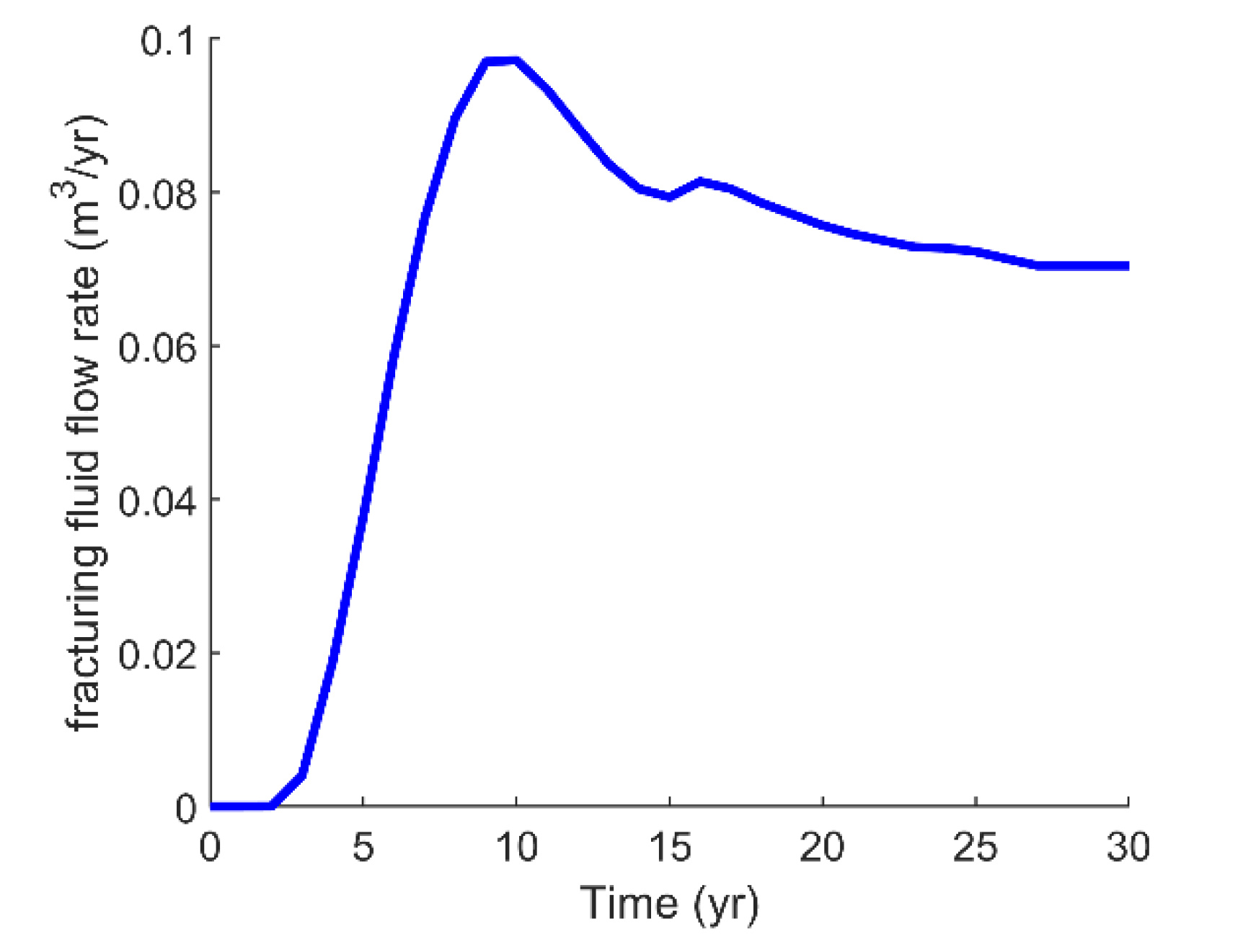
Taherdangkoo et al. [17] conducted an extensive sensitivity analysis on the most influential parameters to examine the extent of fracturing fluid migration from the shale into the overlying aquifers along an abandoned well. They presented their results in terms of fracturing fluid flow rates to the aquifer over 30 years. The parameters studied include fracturing fluid injection rate, shale permeability, shale porosity, overburden thickness, overburden permeability, salinity, effective abandoned well permeability, and its distance to hydraulic fractures. The parameter values used in the base-case model and sensitivity analysis are shown in Table 1. As an example, fracturing fluid flow rate to the aquifer for the base-case model is displayed in Figure 2 [17]. We used fluid flow rates obtained from the sensitivity analysis to build the input dataset, which includes 31-time steps of 24 elements (i.e., model runs). In total, the input dataset contains 744 data records of fracturing fluid flow rate to the aquifer.
Following the ratio of 60:20:20, the input dataset (i.e., fracturing fluid flow rate data) was randomly divided into training, validating, and testing sets. A sample of 446 data was specified for the training phase, 149 data for the validation phase, and the remaining 149 data were used to analyze the reliability and robustness of the NAR network models. The pre-processing step was performed to prepare the data for the training phase, to achieve more consistent and better results. In general, the Levenberg–Marquardt and Bayesian Regularization algorithms work best if the network inputs and feedbacks are in the range of −1 to 1 [25]. Thus, by applying a normalization function, input and feedback values were scaled in the interval (−1,1) and back-transformed in the testing phase.
2.3. NAR Model
The prediction of the incidence of fracturing fluid flow to shallow groundwater is a nonlinear problem. The nonlinear autoregressive (NAR) neural network represents a powerful class of models that has favorable qualities for recognizing time series patterns and nonlinear characteristics. The NAR network is a recurrent dynamic network with feedback connections enclosing layers of the network; thus, the current output depends on the values of past output [51]. The NAR network can be applied to effectively forecasting time series and can be written as follows [32,52,53]:
where is an unknown nonlinear function that can be approximated by the feedforward neural networks during the training process; is the predicted value of the data series of at a discrete time step , represents past values of the series, and is the approximation error of the series y at time . The NAR network is described in Figure 3.
The development of the optimal architecture for the NAR model requires determination of time delays, the number of hidden nodes, the activation function, and an efficient training algorithm. The optimum number of time delays and hidden nodes were obtained through a trial-and-error procedure [32]. The activation function was selected based on Maier and Dandy [54]. Finally, Levenberg–Marquardt and Bayesian Regularization algorithms were applied to train the model.
2.4. Training Algorithms
2.4.1. Levenberg–Marquardt
The Levenberg–Marquardt (LM) algorithm is a back propagation-type algorithm and it has been widely used for training the NAR network because of the fast convergence speed [55,56]. The LM is an effective modification of the Gauss–Newton method that finds the function (either linear or nonlinear) minima over a space of parameters and optimizes the solution [57]. The LM algorithm uses an approximation of the Hessian matrix, given by [58]:
in which represents the weight, is the Jacobian matrix, is the transpose matrix of , and is the Hessian matrix. represents the learning matrix, and and are the learning coefficient and vector of network errors, respectively. The parameter is automatically updated based on the error at each iteration to secure the convergence. We used a random value of to initiate the iteration process for optimizing weights with the LM algorithm.
2.4.2. Bayesian Regularization
Bayesian Regularization (BR), introduced by MacKay [59], is a mathematical technique for converting nonlinear systems into ‘‘well posed’’ problems [60]. The BR network reduces the potential for overfitting in the training phase while eliminating the need for the validation phase. Thus, BR is especially suitable for small datasets because more data are available for the training [60,61]. The BR automatically sets the best performance function to accomplish an efficient generalization on the basis of Bayesian inference. The determination of the optimal regularization parameters depends upon the computation of the Hessian matrix at the minimum point [62,63]. In this work, a Gauss–Newton approximation of the Hessian matrix is applied to optimize regularization [62].
2.5. Network Architecture
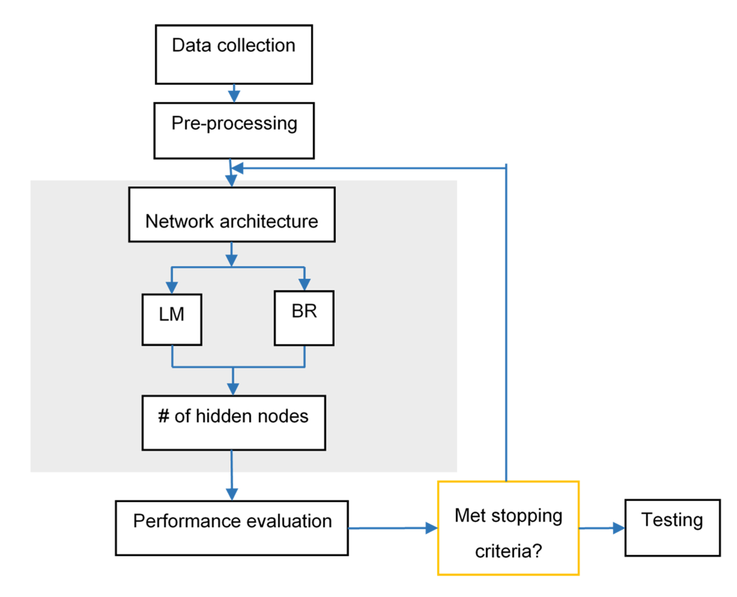
The NAR network employed is a feed forward neural network with three layers, namely input, hidden and output layers (Figure 3). Sigmoid function, a continuous non-linear function, is the most commonly used activation function for neural network design with back propagation training. The activation functions in hidden and output layers are logistic sigmoid and linear, respectively. A trial-and-error procedure is carried out to determine the number of nodes in the hidden layer and value of time delays in order to generate accurate model responses. The Levenberg–Marquardt and Bayesian Regularization algorithms were employed for training of the NAR network and their performance were evaluated under the same network structure. The necessary steps to implement the network is illustrated in Figure 4.
The NAR neural network is trained in a series–parallel configuration. In the training phase, the true output is available and it was used as the input to the network. During the testing phase, the calculated output was fed back to the network to estimate the next value of the output in a parallel configuration. In this study, the initial weights in the network are assigned randomly and they were adjusted at each iteration (i.e., epoch) to reduce the error. The procedure continued until the network output met the stopping criteria.
2.6. Performance Evaluation
The prediction performance of the models was evaluated by two well-known statistical criteria, namely the coefficient of determination (R2) and mean squared errors (MSE). R2 is a linear regression used to analyze the best fit between the measured values and model’s predicted values, given by:
in which and represent the measured and predicted values, respectively, stands for the average of measured values, and n equals the number of values. The MSE calculates the average squared difference between the measured and predicted values, given by the following equation:
3. Results and Discussion
This study considers the failure scenario of upward migration of fracturing fluid from the shale formation into a shallow aquifer along an abandoned well. We employed a NAR network model to predict the incident of fracturing fluid in the aquifer. The NAR network has one input, i.e., the fracturing fluid flow rate into the aquifer, and it generates one output that is the prediction of flow rate at a certain time ahead. We used the logistic sigmoid and linear activation functions at the hidden and output layers respectively because the modeling problem presented here is a function approximation problem. The error analysis showed that the network with three nodes in the hidden layer and two time delays provide the best performance.
Figure 5 shows the results of the error autocorrelation function of the fracturing fluid flow rate. This function describes the relationship between the prediction errors and time, and it was used to determine the value of time delays in the NAR network. To obtain a perfect training fit, there should be only one nonzero value over the entire function. As shown for the current network structure (node = 3 and delay = 2), error autocorrelations were approximately in the 95% confidence interval zone, except for the ones at zero lag, thus NAR-LM and NAR-BR models are adequate. The calculated MSE and R2 for the training phase (Table 2) show that both models reached the best fitting performances in terms of evaluation criteria. For instance, R2 values of higher than 0.99 indicated a strong correlation between the measured values and fitting values. According to Figure 5 and Table 2, we conclude that a sample of 446 data is adequate to train the NAR models.
An open-loop architecture (series–parallel configuration) is more useful for training the NAR network, while a closed-loop architecture (parallel configuration) is suitable for multiple-step-ahead predictions [31]. We used a transfer function to convert the network into the closed-loop after finishing the open-loop training. The prediction ability of the models in terms of evaluation indices is summarized in Table 2. Note that the NAR-BR model does not require a validation phase. The testing results were similar to those of training: for example, R2 values higher than 0.9 for the testing phase indicated the satisfactory performance of both developed models. For further comparison of evaluation indices, MSE of NAR-LM and NAR-BAR were 4.2 × 10⁻⁴ and 2.4 × 10⁻⁴ respectively, which proved the strong ability of the developed models in predicting the nonlinear behavior of fracturing fluid flow to the aquifer. The results suggest that NAR-BR model has a slightly better prediction performance compared with that of the NAR-LM model in terms of larger R2 and smaller MSE.
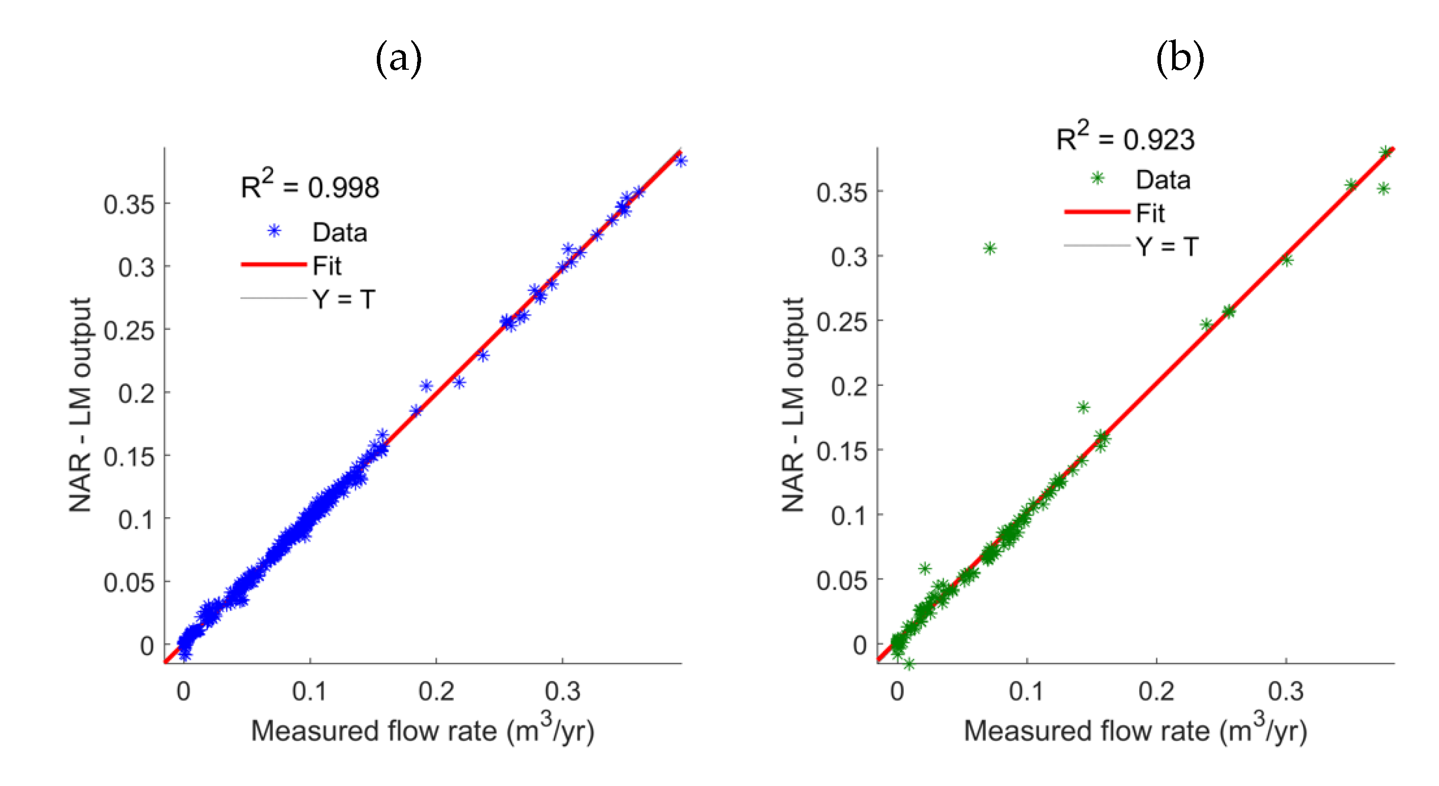
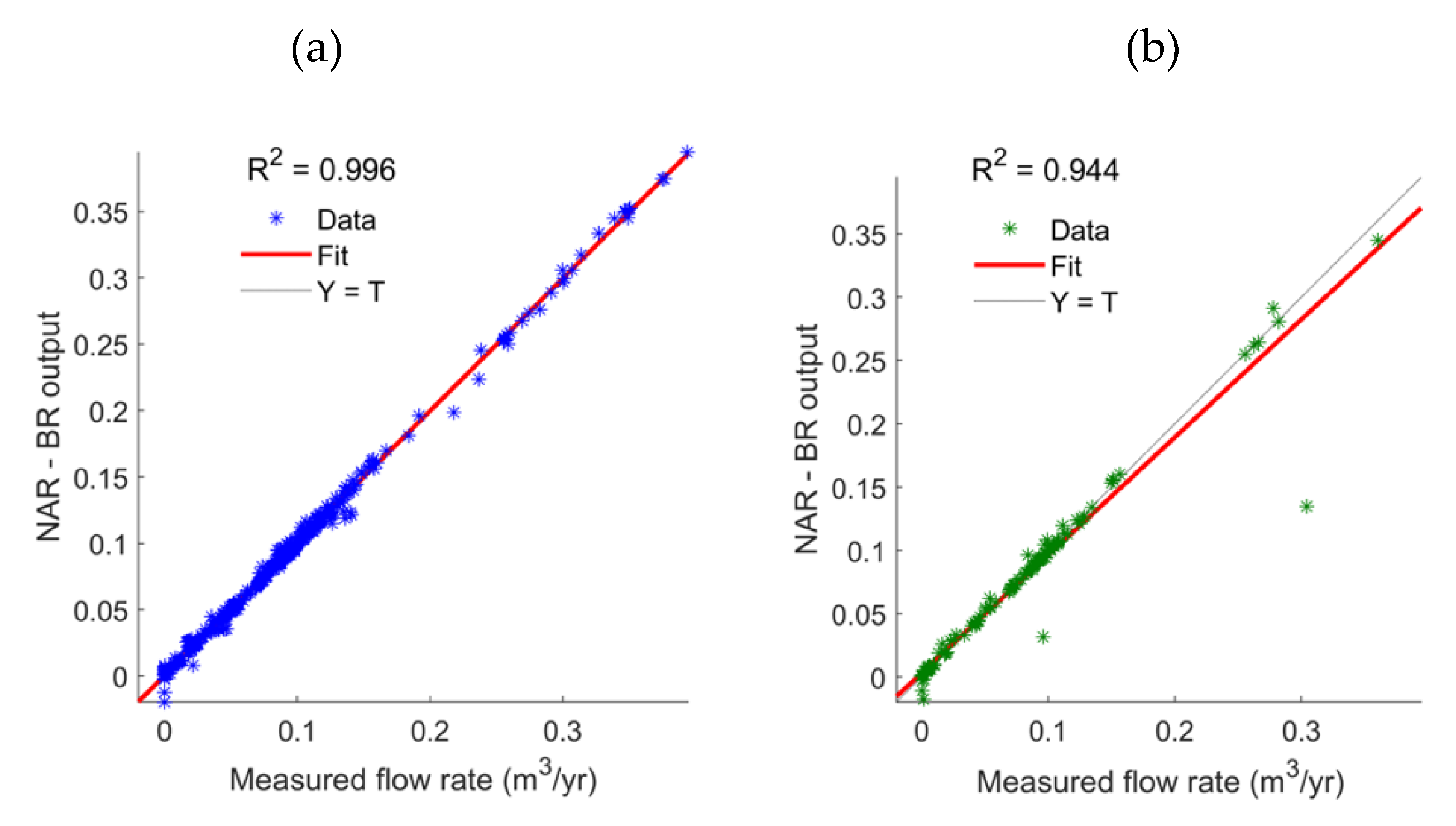
The scatter diagrams of the measured and predicted flow rate values by NAR-LM and NAR-BR networks are illustrated in Figure 6 and Figure 7, respectively. We also plotted a 45-degree reference line. The measured and predicted data should lie close to the reference line to demonstrate a very good model fit. For the training phase, this can be seen in Figure 6a and Figure 7a, indicating that both models fit equally well statistically. Figure 6b and Figure 7b displayed acceptable fit, which indicates good predictive abilities of both models for new datasets. Although the predicted values of the NAR-LM model fit better to the reference line, R2 value of the NAR-BR model is slightly higher.
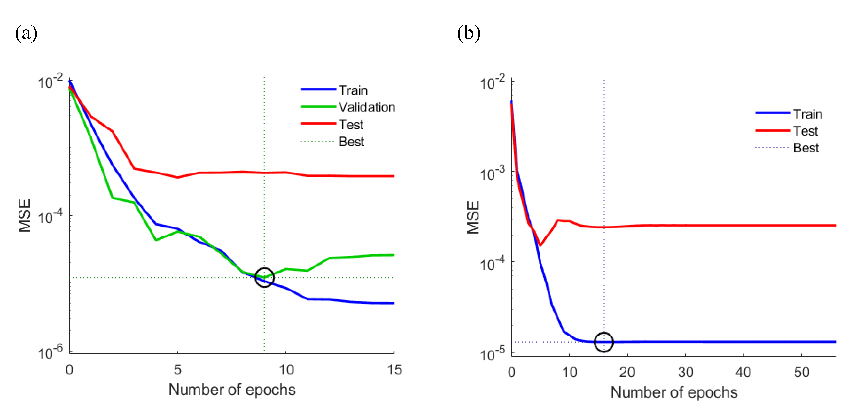
The performance plots of the NAR-LM and NAR-BR models are shown in Figure 8. This figure illustrates the relationship between the testing, training, and validation phases in predicting fluid flow rates into the aquifer, in terms of MSE versus number of epochs. The black circle in Figure 8a shows the performance of the NAR-LM model, which performed the best during the validation process. The black circle in Figure 8b shows the performance of the NAR-BR model, which was the best one during the testing phase. As illustrated in Figure 8, the best performance for the validation phase is 1.2 × 10⁻⁵ at epoch 9 for the NAR-LM model, while the NAR-BR model experiences the best performance (MSE = 1.3 × 10⁻⁵) for the training phase at epoch 16.
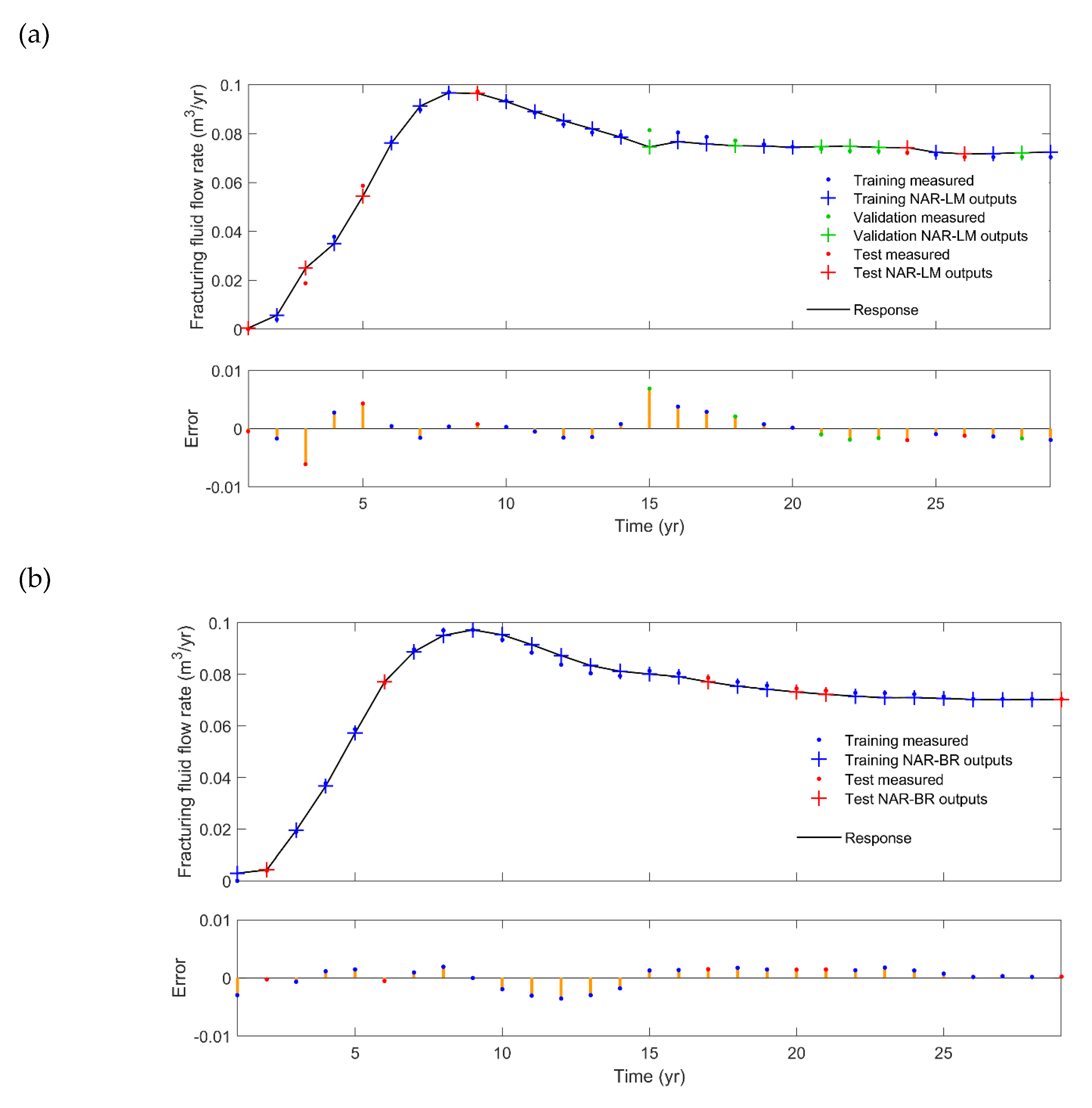
Figure 9 illustrates the visualized comparison results of fracturing fluid flow rate predictions for the training, validation, and testing phases. Note that the response line in this figure is the fracturing fluid flow rate to the aquifer, which is also presented in Figure 2. It was observed that the predicted fluid flow rate values followed the measured pattern. The differences between predicted and measured values are small (± 7 × 10⁻³ m3/year) for the entire time period, indicating that the NAR-LM and NAR-BR models were able to efficiently predict fracturing fluid flow rate to the aquifer over the simulation period. Comparing the response lines and error plots of this figure further indicated the superior performance of the NAR-BR model.
The arrival time of fracturing fluid to shallow groundwater highly depends on the geological and hydrogeological characteristics of the formations between the aquifer and hydrocarbon reservoirs. Evaluating the frequency and impact of fracturing fluid leaks requires extended periods of water-quality monitoring, particularly in cases where overburden layers are not highly fractured and preferential flow paths (e.g., faults and leaky abandoned wells) are not in the vicinity of the operation. Efforts are underway to identify the relationship between oil and gas operations and groundwater contamination in many regions. NAR models could be used for quick and inexpensive but effective assessment of the potential impacts of hydraulic fracturing in the absence of adequate field or modeling data. The results demonstrate that the NAR network trained with LM and BR algorithms could efficiently identify time series patterns in existing fracturing fluid flow rate data to accurately predict the unseen values.
Interdisciplinary research has become necessary to break new grounds in the science of fluid migration from hydrocarbon formations to groundwater. Our results further highlight the need for strengthening the interdisciplinary collaborations to link petrophysical, geomechanical and hydrogeological information to develop data-driven models to better evaluate the impact of contaminant leakage to groundwater systems, which may occur by vertical flow migration along pre-existing permeable pathways. Data-driven models have a high potential to recognize the contamination problems, in particular when dealing with high data uncertainty, and missing and sparse information. For instance, data-driven models can be helpful for assessing regional trends of incidents of groundwater contamination, as the availability of consistent data is limited at the regional scale. Additional research is essential to build the confidence in the applicability of the methodology and assessing the risks of hydraulic fracturing.
4. Conclusions
We presented a novel application of a NAR neural network to predict fracturing fluid flow rate into a shallow aquifer following hydraulic fracturing. The dataset used for the network development was taken from Taherdangkoo et al. [17] and included 744 records of fracturing fluid flow rate into the aquifer, resulting from the upward migration along an abandoned well. Based on the literature review on the performance of training algorithms, the Levenberg–Marquardt and Bayesian Regularization algorithms were selected to train the NAR model. The network structure with three nodes in the hidden layer and two time delays provided the optimal performance.
The results indicated the high accuracy and reliability of NAR-LM and NAR-BR models in the prediction of fracturing fluid flow rate to the aquifer, particularly when using a limited dataset. Both NAR models provides excellent results in terms of goodness-of-fit and independence test. The advantage and power of the proposed models are the fast, cheap and effective approach of calculation in comparison with traditional modeling approaches. By comparing the modeling results, we demonstrated that the predictive performance of the NAR-BR model is slightly better than the NAR-LM model.
There are a few incidents where fracturing fluid and methane were reported to contaminate the aquifer. The NAR models can serve as an additional tool to analyze the incidents of groundwater contamination, especially regional trends of occurrence. In summary, the NAR models trained with LM and BR algorithms showed to have considerable potential in assisting the development of water-quality monitoring programs in the oil and gas regions.
Author Contributions
Conceptualization, R.T., A.T, and M.T; methodology, R.T and M.T.; formal analysis, R.T.; writing—original draft preparation, R.T.; writing—review and editing, R.T, A.T., M.T., P.Q., and M.S. All authors have read and agreed to the published version of the manuscript.
Funding
We acknowledge the funding received from the European Union’s Horizon 2020 Research and Innovation program. Project: “Furthering the knowledge Base for Reducing the Environmental Footprint of Shale Gas Development” FracRisk, grant agreement 636811. We further acknowledge the support by the Open Access Grant Program of the German Research Foundation (DFG) and the Open Access Publication Fund of the University of Göttingen.
Acknowledgments
The authors would like to thank Marco Fazio (University of Göttingen) and two anonymous reviewers for their critical insights and constructive reviews.
Conflicts of Interest
The authors declare no conflicts of interest.
References
- Cook, T.; Perrin, J.; Wagener, D.V. Hydraulically Fractured Horizontal Wells Account for Most New Oil and Natural Gas Wells. Available online: https://www.eia.gov/todayinenergy/detail.php?id=34732 (accessed on 30 January 2018).
- Tatomir, A.; McDermott, C.; Bensabat, J.; Class, H.; Edlmann, K.; Taherdangkoo, R.; Sauter, M. Conceptual model development using a generic Features, Events, and Processes (FEP) database for assessing the potential impact of hydraulic fracturing on groundwater aquifers. Adv. Geosci. 2018, 45, 185–192. [Google Scholar] [CrossRef] [Green Version]
- Vengosh, A.; Jackson, R.; Warner, N. A critical review of the risks to water resources from unconventional shale gas development and hydraulic fracturing in the United States. Sci. Technol. 2014, 48, 8334–8348. [Google Scholar] [CrossRef] [PubMed]
- Sauter, M.; Brosig, K.; Lange, T.; Jahnke, W.; Helmig, R.; Kissinger, A.; Heitfeld, M.; Kluenker, J.; Schetelig, K. Risiken im Geologischen System bei der Fracking-Technologie Abschätzung der Auswirkungen auf Grundwasservorkommen. Wasser und Abfall 2012, 14, 16. [Google Scholar]
- Rice, A.K.; Lackey, G.; Proctor, J.; Singha, K. Groundwater-quality hazards of methane leakage from hydrocarbon wells: A review of observational and numerical studies and four testable hypotheses. Wiley Interdiscip. Rev. Water 2018, 5, e1283. [Google Scholar] [CrossRef]
- Lange, T.; Sauter, M.; Heitfeld, M.; Schetelig, K.; Brosig, K.; Jahnke, W.; Kissinger, A.; Helmig, R.; Ebigbo, A.; Class, H. Hydraulic fracturing in unconventional gas reservoirs: Risks in the geological system part 1. Environ. Earth Sci. 2013, 70, 3839–3853. [Google Scholar] [CrossRef]
- Gassiat, C.; Gleeson, T.; Lefebvre, R.; McKenzie, J. Hydraulic fracturing in faulted sedimentary basins: Numerical simulation of potential contamination of shallow aquifers over long time scales. Water Resour. Res. 2013, 49, 8310–8327. [Google Scholar] [CrossRef] [Green Version]
- Myers, T. Potential Contaminant Pathways from Hydraulically Fractured Shale to Aquifers. Groundwater 2012, 50, 872–882. [Google Scholar] [CrossRef] [PubMed]
- Nowamooz, A.; Lemieux, J.-M.; Molson, J.; Therrien, R. Numerical investigation of methane and formation fluid leakage along the casing of a decommissioned shale gas well. Water Resour. Res. 2015, 51, 4592–4622. [Google Scholar] [CrossRef] [Green Version]
- Taherdangkoo, R.; Tatomir, A.; Taylor, R.; Sauter, M. Numerical investigations of upward migration of fracking fluid along a fault zone during and after stimulation. Energy Procedia 2017, 125, 126–135. [Google Scholar] [CrossRef]
- Birdsell, D.T.; Rajaram, H.; Dempsey, D.; Viswanathan, H.S. Hydraulic fracturing fluid migration in the subsurface: A review and expanded modeling results. Water Resour. Res. 2015, 51, 7159–7188. [Google Scholar] [CrossRef]
- Reagan, M.T.; Moridis, G.J.; Keen, N.D.; Johnson, J.N. Numerical simulation of the environmental impact of hydraulic fracturing of tight/shale gas reservoirs on near-surface groundwater: Background, base cases, shallow reservoirs, short-term gas, and water transport. Water Resour. Res. 2015, 4, 2543–2573. [Google Scholar] [CrossRef] [PubMed]
- Brownlow, J.W.; James, S.C.; Yelderman, J.C. Influence of Hydraulic Fracturing on Overlying Aquifers in the Presence of Leaky Abandoned Wells. Groundwater 2016, 54, 781–792. [Google Scholar] [CrossRef] [PubMed]
- King, G.E.; Rainbolt, M.F.; Swanson, C. Frac Hit Induced Production Losses: Evaluating Root Causes, Damage Location, Possible Prevention Methods and Success of Remedial Treatments. In Proceedings of the SPE Annual Technical Conference and Exhibition, San Antonio, TX, USA, 9–11 October 2017. [Google Scholar]
- Gasda, S.E.; Bachu, S.; Celia, M.A. Spatial characterization of the location of potentially leaky wells penetrating a deep saline aquifer in a mature sedimentary basin. Environ. Geol. 2004, 46, 707–720. [Google Scholar] [CrossRef]
- Gasda, S.E.; Celia, M.A.; Wang, J.Z.; Duguid, A. Wellbore permeability estimates from vertical interference testing of existing wells. Energy Procedia 2013, 37, 5673–5680. [Google Scholar] [CrossRef] [Green Version]
- Taherdangkoo, R.; Tatomir, A.; Anighoro, T.; Sauter, M. Modeling fate and transport of hydraulic fracturing fluid in the presence of abandoned wells. J. Contam. Hydrol. 2019, 221, 58–68. [Google Scholar] [CrossRef] [PubMed]
- Flewelling, S.A.; Sharma, M. Constraints on upward migration of hydraulic fracturing fluid and brine. Groundwater 2014, 52, 9–19. [Google Scholar] [CrossRef] [Green Version]
- Birdsell, D.T.; Rajaram, H.; Lackey, G. Imbibition of hydraulic fracturing fluids into partially saturated shale. Water Resour. Res. 2015, 51, 6787–6796. [Google Scholar] [CrossRef]
- Edwards, R.W.J.; Doster, F.; Celia, M.A.; Bandilla, K.W. Numerical modeling of gas and water flow in shale gas formations with a focus on the fate of hydraulic fracturing fluid. Environ. Sci. Technol. 2017, 51, 13779–13787. [Google Scholar] [CrossRef]
- Pfunt, H.; Houben, G.; Himmelsbach, T. Numerical modeling of fracking fluid migration through fault zones and fractures in the North German Basin. Hydrogeol. J. 2016, 24, 1343–1358. [Google Scholar] [CrossRef]
- Osborn, S.G.; Vengosh, A.; Warner, N.R.; Jackson, R.B. Methane contamination of drinking water accompanying gas-well drilling and hydraulic fracturing. Proc. Natl. Acad. Sci. USA 2011, 108, 8172–8176. [Google Scholar] [CrossRef] [Green Version]
- Kissinger, A.; Helmig, R.; Ebigbo, A.; Class, H.; Lange, T.; Sauter, M.; Heitfeld, M.; Klünker, J.; Jahnke, W. Hydraulic fracturing in unconventional gas reservoirs: Risks in the geological system, part 2: Modelling the transport of fracturing fluids, brine and methane. Environ. Earth Sci. 2013, 70, 3855–3873. [Google Scholar] [CrossRef]
- Cao, V.; Schaffer, M.; Taherdangkoo, R.; Licha, T. Solute reactive tracers for hydrogeological applications: A short review and future prospects. Water 2020, 12, 653. [Google Scholar] [CrossRef] [Green Version]
- Guzman, S.M.; Paz, J.O.; Tagert, M.L.M. The use of NARX neural networks to forecast daily groundwater levels. Water Resour. Manag. 2017, 31, 1591–1603. [Google Scholar] [CrossRef]
- Loucks, D.P.; Van Beek, E. Water Resources Systems Planning and Management: An Introduction to Methods, Models and Applications. Available online: https://hydrologie.org/BIB/Publ_UNESCO/SR_999_E_2005.pdf (accessed on 15 March 2020).
- Kisi, O.; Cigizoglu, H.K. Comparison of different ANN techniques in river flow prediction. Civ. Eng. Environ. Syst. 2007, 24, 211–231. [Google Scholar] [CrossRef]
- Olyaie, E.; Banejad, H.; Chau, K.W.; Melesse, A.M. A comparison of various artificial intelligence approaches performance for estimating suspended sediment load of river systems: A case study in United States. Environ. Monit. Assess. 2015, 187, 189. [Google Scholar] [CrossRef]
- Zhang, Q.; Stanley, S.J. Forecasting raw-water quality parameters for the north Saskatchewan river by neural network modeling. Water Res. 1997, 31, 2340–2350. [Google Scholar] [CrossRef]
- Maier, H.R.; Dandy, G.C. The Use of Artificial Neural Networks for the Prediction of Water Quality Parameters. Water Resour. Res. 1996, 32, 1013–1022. [Google Scholar] [CrossRef]
- Wei, S.; Zuo, D.; Song, J. Improving prediction accuracy of river discharge time series using a Wavelet-NAR artificial neural network. J. Hydroinformatics 2012, 14, 974–991. [Google Scholar] [CrossRef] [Green Version]
- Ruiz, L.; Cuéllar, M.; Calvo-Flores, M.; Jiménez, M. An application of non-linear autoregressive neural networks to predict energy consumption in public buildings. Energies 2016, 9, 684. [Google Scholar] [CrossRef] [Green Version]
- Adamowski, J.; Fung Chan, H.; Prasher, S.O.; Ozga-Zielinski, B.; Sliusarieva, A. Comparison of multiple linear and nonlinear regression, autoregressive integrated moving average, artificial neural network, and wavelet artificial neural network methods for urban water demand forecasting in Montreal, Canada. Water Resour. Res. 2012, 48, 1–14. [Google Scholar] [CrossRef]
- Neuzil, C.E. How permeable are clays and shales? Water Resour. Res. 1994, 30, 145–150. [Google Scholar] [CrossRef]
- Edwards, R.W.; Celia, M.A. Shale gas well, hydraulic fracturing, and formation data to support modeling of gas and water flow in shale formations. Water Resour. Res. 2018, 54, 3196–3206. [Google Scholar] [CrossRef]
- Freeze, R.A.; Cherry, J.A. Groundwater prentice-hall. Eaglewood Cliffs 1979, 176, 161–177. [Google Scholar]
- Gleeson, T.; Smith, L.; Moosdorf, N.; Hartmann, J.; Dürr, H.H.; Manning, A.H.; van Beek, L.P.H.; Jellinek, A.M. Mapping permeability over the surface of the Earth. Geophys. Res. Lett. 2011, 38, L02401. [Google Scholar] [CrossRef] [Green Version]
- Luijendijk, E.; Gleeson, T. How well can we predict permeability in sedimentary basins? Deriving and evaluating porosity-permeability equations for noncemented sand and clay mixtures. Geofluids 2015, 15, 67–83. [Google Scholar] [CrossRef] [Green Version]
- EIA. World Shale Gas Resources: An Initial Assessment of 14 Regions Outside the United States; US Department of Energy: Washington, DC, USA, 2011. [Google Scholar]
- EIA. Review of Emerging Resources: US Shale Gas and Shale Oil Plays; US Department of Energy: Washington, DC, USA, 2011. [Google Scholar]
- Magri, F.; Bayer, U.; Jahnke, C.; Clausnitzer, V.; Diersch, H.J.; Fuhrman, J.; Möller, P.; Pekdeger, A.; Tesmer, M.; Voigt, H.J. Fluid-dynamics driving saline water in the North East German Basin. Int. J. Earth Sci. 2005, 94, 1056–1069. [Google Scholar] [CrossRef]
- Kissinger, A.; Noack, V.; Knopf, S.; Konrad, W.; Scheer, D.; Class, H. Regional-scale brine migration along vertical pathways due to CO2 injection--Part 2: A simulated case study in the North German Basin. Hydrol. Earth Syst. Sci. 2017, 21, 2751–2775. [Google Scholar] [CrossRef] [Green Version]
- Nogues, J.P.; Nordbotten, J.M.; Celia, M.A. Detecting leakage of brine or CO2 through abandoned wells in a geological sequestration operation using pressure monitoring wells. Energy Procedia 2011, 4, 3620–3627. [Google Scholar] [CrossRef] [Green Version]
- Bai, M.; Reinicke, K. In Numerical Simulation of CO2 Leakage through Abandoned Wells during CO2 Underground Storage, Proceedings of the Clean Energy Systems in the Subsurface: Production, Storage and Conversion, Goslar, Germany, 21–23 May 2013; Springer: Berlin/Heidelberg, Germany, 2013; pp. 197–210. [Google Scholar]
- Pawar, R.J.; Watson, T.L.; Gable, C.W. Numerical simulation of CO2 leakage through abandoned wells: Model for an abandoned site with observed gas migration in Alberta, Canada. Energy Procedia 2009, 1, 3625–3632. [Google Scholar] [CrossRef] [Green Version]
- Gasda, S.E.; Nordbotten, J.M.; Celia, M.A. Determining effective wellbore permeability from a field pressure test: A numerical analysis of detection limits. Environ. Geol. 2008, 54, 1207–1215. [Google Scholar] [CrossRef]
- Nordbotten, J.M.; Celia, M.A.; Bachu, S.; Dahle, H.K. Semianalytical solution for CO2 leakage through an abandoned well. Environ. Sci. Technol. 2005, 39, 602–611. [Google Scholar] [CrossRef] [PubMed]
- Nordbotten, J.M.; Celia, M.A.; Bachu, S. Analytical solutions for leakage rates through abandoned wells. Water Resour. Res. 2004, 40, W04204. [Google Scholar] [CrossRef]
- Ebigbo, A.; Class, H.; Helmig, R. CO2 leakage through an abandoned well: Problem-oriented benchmarks. Comput. Geosci. 2007, 11, 103–115. [Google Scholar] [CrossRef]
- Celia, M.A.; Bachu, S.; Nordbotten, J.M.; Gasda, S.E.; Dahle, H.K. Quantitative estimation of CO 2 leakage from geological storage: Analytical models, numerical models, and data needs. Greenh. Gas Control Technol. 7 2005, I, 663–671. [Google Scholar]
- Da Costa Lopes, F.; Watanabe, E.H.; Rolim, L.G.B. A control-oriented model of a PEM fuel cell stack based on NARX and NOE neural networks. IEEE Trans. Ind. Electron. 2015, 62, 5155–5163. [Google Scholar] [CrossRef]
- López, M.; Valero, S.; Senabre, C.; Aparicio, J.; Gabaldon, A. Application of SOM neural networks to short-term load forecasting: The Spanish electricity market case study. Electr. Power Syst. Res. 2012, 91, 18–27. [Google Scholar] [CrossRef]
- Wang, K.W.; Deng, C.; Li, J.P.; Zhang, Y.Y.; Li, X.Y.; Wu, M.C. Hybrid methodology for tuberculosis incidence time-series forecasting based on ARIMA and a NAR neural network. Epidemiol. Infect. 2017, 145, 1118–1129. [Google Scholar] [CrossRef] [Green Version]
- Maier, H.R.; Dandy, G.C. Neural networks for the prediction and forecasting of water resources variables: A review of modelling issues and applications. Environ. Model. Softw. 2000, 15, 101–124. [Google Scholar] [CrossRef]
- Hagan, M.T.; Menhaj, M.B. Training Feedforward Networks with the Marquardt Algorithm. IEEE Trans. Neural Netwrok 1994, 5, 989–993. [Google Scholar] [CrossRef]
- Marquardt, D.W. An Algorithm for Least-Squares Estimation of Nonlinear Parameters. J. Soc. Ind. Appl. Math. 1963, 11, 431–441. [Google Scholar] [CrossRef]
- Sahoo, S.; Jha, M.K. Groundwater-level prediction using multiple linear regression and artificial neural network techniques: A comparative assessment. Hydrogeol. J. 2013, 21, 1865–1887. [Google Scholar] [CrossRef]
- Bishop, C. Neural Networks for Pattern Recognition; Oxford University Press: Oxford, UK, 1995. [Google Scholar]
- MacKay, D.J.C. Bayesian Interpolation. Neural Comput. 1992, 4, 415–447. [Google Scholar] [CrossRef]
- Burden, F.; Winkler, D. Bayesian regularization of neural networks. Methods Mol. Biol. 2008, 458, 25–44. [Google Scholar] [PubMed]
- Doan, C.D.; Liong, S.Y. Generalization for multilayer neural network bayesian regularization or early stopping. In Proceedings of the Asia Pacific Association of Hydrology and Water Resources 2nd Conference, Singapore, Singapore, 5–8 July 2004; pp. 5–8. [Google Scholar]
- Foresee, F.; Hagan, M.T. Gauss-Newton approximation to bayesian learning. In Proceedings of the IEEE International Conference on Neural Networks–Conference Proceedings, Houston, TX, USA, 12 June 1997; pp. 1930–1935. [Google Scholar]
- MacKay, D.J.C. A practical bayesian framework for backpropagation networks. Neural Comput. 1992, 4, 448–472. [Google Scholar] [CrossRef]
Figure 1.
The conceptual model used for simulations in Taherdangkoo et al. [17].
Figure 1.
The conceptual model used for simulations in Taherdangkoo et al. [17].

Figure 2.
Fracturing fluid flow rate to the aquifer for the base-case model during the simulation time.
Figure 2.
Fracturing fluid flow rate to the aquifer for the base-case model during the simulation time.

Figure 3.
A sketch of a standard nonlinear autoregressive (NAR) neural network.

Figure 4.
A basic procedure for the NAR network training.

Figure 5.
Error autocorrelations of (a) NAR-LM and (b) NAR-BR models for the training phase.

Figure 6.
Performance of the NAR-LM model for the prediction of fracturing fluid flow rate to the aquifer: (a) training and (b) testing.
Figure 6.
Performance of the NAR-LM model for the prediction of fracturing fluid flow rate to the aquifer: (a) training and (b) testing.

Figure 7.
Performance of the NAR-BR model for the prediction of fracturing fluid flow rate to the aquifer: (a) training and (b) testing.
Figure 7.
Performance of the NAR-BR model for the prediction of fracturing fluid flow rate to the aquifer: (a) training and (b) testing.

Figure 8.
Convergence plots of the NAR models in terms of number of epochs: (a) NAR-LM and (b) NAR-BR.
Figure 8.
Convergence plots of the NAR models in terms of number of epochs: (a) NAR-LM and (b) NAR-BR.

Figure 9.
Response of (a) NAR-LM and (b) NAR-BR models in predicting fracturing fluid flow rate to the shallow aquifer. The top panels show the modeled fluid flow rate presented in Figure 2. The bottom panels display the model’s performance error in the training, validation, and testing phases.
Figure 9.
Response of (a) NAR-LM and (b) NAR-BR models in predicting fracturing fluid flow rate to the shallow aquifer. The top panels show the modeled fluid flow rate presented in Figure 2. The bottom panels display the model’s performance error in the training, validation, and testing phases.


Table 1.
Parameters used in base-case model and sensitivity analysis simulations [17].
Table 1.
Parameters used in base-case model and sensitivity analysis simulations [17].
| Parameter | Unit | Base-Case Value | Min. | Max. | Source |
|---|---|---|---|---|---|
| Shale permeability | m2 | 1 × 10⁻¹⁹ | 1 × 10⁻²¹ | 1 × 10⁻¹⁸ | [12,13,34] |
| Shale porosity | 0.01 | 0.01 | 0.05 | [7,34,35,36] | |
| Overburden permeability | m2 | Depth-dependent | 1 × 10⁻¹⁷ | 1 × 10⁻¹⁵ | [7,37,38] |
| Overburden thickness | m | 1600 | 900 | 2900 | [7,39,40] |
| Salinity gradient | g/lm | 0.15 | 0.1 | 0.2 | [41,42] |
| Fracturing fluid volume | m3 | 11,365 | 11,000 | 15,000 | [8,11,13] |
| Abandoned well permeability | m2 | 1 × 10⁻¹² | 1 × 10⁻¹⁷ | 1 × 10⁻¹² | [43,44,45,46,47,48,49,50] |
| Distance of fracture plane to well | m | 0 | 0 | 15 |
Table 2.
Evaluation of the NAR-LM and NAR-BR models’ performances.
| Statistical Parameter | NAR-LM | NAR-BR | |||
|---|---|---|---|---|---|
| Training | Validation | Testing | Training | Testing | |
| R2 | 0.998 | 0.996 | 0.923 | 0.996 | 0.944 |
| MSE | 1.07 × 10⁻⁵ | 1.2 × 10⁻⁵ | 4.2 × 10⁻⁴ | 1.3 × 10⁻⁵ | 2.4 × 10⁻⁴ |
© 2020 by the authors. Licensee MDPI, Basel, Switzerland. This article is an open access article distributed under the terms and conditions of the Creative Commons Attribution (CC BY) license (http://creativecommons.org/licenses/by/4.0/).
Share and Cite
MDPI and ACS Style
Taherdangkoo, R.; Tatomir, A.; Taherdangkoo, M.; Qiu, P.; Sauter, M. Nonlinear Autoregressive Neural Networks to Predict Hydraulic Fracturing Fluid Leakage into Shallow Groundwater. Water 2020, 12, 841. https://doi.org/10.3390/w12030841
AMA Style
Taherdangkoo R, Tatomir A, Taherdangkoo M, Qiu P, Sauter M. Nonlinear Autoregressive Neural Networks to Predict Hydraulic Fracturing Fluid Leakage into Shallow Groundwater. Water. 2020; 12(3):841. https://doi.org/10.3390/w12030841
Chicago/Turabian StyleTaherdangkoo, Reza, Alexandru Tatomir, Mohammad Taherdangkoo, Pengxiang Qiu, and Martin Sauter. 2020. "Nonlinear Autoregressive Neural Networks to Predict Hydraulic Fracturing Fluid Leakage into Shallow Groundwater" Water 12, no. 3: 841. https://doi.org/10.3390/w12030841
Note that from the first issue of 2016, this journal uses article numbers instead of page numbers. See further details here.