Spatial Variation in Aragonite Saturation State and the Influencing Factors in Jiaozhou Bay, China


1
Department of Environment Science, College of Resource and Environment, Shanxi Agricultural University, Taigu 030801, China
2
Key Laboratory of Marine Environmental Science and Ecology, Ministry of Education, College of Environmental Science and Engineering, Ocean University of China, Qingdao 266100, China
3
Center for Ocean and Climate Research, First Institute of Oceanography, SOA, Qingdao 266061, China
4
Department of Geography and Environmental Science, University of Reading, Whiteknights, Reading RG6 6AB, UK
*
Authors to whom correspondence should be addressed.
Water 2020, 12(3), 825; https://doi.org/10.3390/w12030825
Submission received: 17 December 2019
/
Revised: 26 February 2020
/
Accepted: 8 March 2020
/
Published: 14 March 2020
(This article belongs to the Special Issue The Impact of Climate Change and Human Activities on Aquatic Environments)
Abstract
:Both natural processes and human activities affect seawater calcium carbonate saturation state (Ωarag), while the mechanisms are still far from being clearly understood. This study analysed the seawater surface Ωarag during summer and winter in Jiaozhou Bay (JZB), China, based on two cruises observations performed in January and June 2017. The ranges of Ωarag values were 1.55~2.92 in summer and 1.62~2.15 in winter. Regression analyses were conducted to identify the drivers of the change of Ωarag distribution, and then the relative contributions of temperature, mixing processes and biological processes to the spatial differences in Ωarag were evaluated by introducing the difference between total alkalinity (TA) and dissolved inorganic carbon (DIC) as a proxy for Ωarag. The results showed that biological processes were the main factor affecting the spatial differences in Ωarag, with relative contributions of 70% in summer and 50% in winter. The contributions of temperature (25% in summer and 20% in winter) and the mixing processes (5% in summer and 30% in winter) were lower. The increasing urbanization in offshore areas can further worsen acidification, therefore environmental protection in both offshore and onshore is needed.
1. Introduction
Ocean acidification (OA) not only causes physical and chemical changes in the ocean but is also of widespread concern due to its serious impact on marine ecosystems and calcifying organisms [1,2,3,4]. Coastal waters are the most active areas for fishery production and shellfish farming, and studies related to OA mechanisms are a top priority in the region [5,6,7]. Unlike the open ocean, nearshore acidification is not only affected by global OA caused by increasing atmospheric CO2 levels but also by the coupled effects of various processes, such as upwelling, organic matter degradation, primary production of phytoplankton and river input, due to the strong interaction between land and ocean, making the acidification mechanism in coastal waters more complicated [8,9,10,11]. In bays, which are highly affected by human disturbance, the mutual enhancement, interference and superimposition of the effects of the above processes are especially prominent. Therefore, clarifying the OA mechanism in this region will be helpful for understanding the OA process in coastal waters under the coupled influence of natural processes and human activities, and will be of great significance for predicting the developing trend and impact of OA and formulating appropriate mitigation measures in coastal waters.
Compared with pH and carbonate ion concentration ([CO32−]), calcium carbonate saturation (Ω) is more directly indicative of the effect of acidification on biocalcification [12,13]. Ω is defined as the product of calcium and carbonate ion concentrations divided by the apparent solubility product (Ksp*) of calcium carbonate, i.e., Ω = [Ca2+] [CO32−]/Ksp* [14]. When Ω < 1.0, waters are undersaturated with respect to carbonate minerals, and the outer shell and skeleton of the organism should dissolve [15,16]. Calcite and aragonite are the main existing forms of CaCO3 in the marine environment. The solubility of aragonite is about 50% higher than that of calcite at 25 °C [17], and aragonite is usually the most abundant carbonate mineral in the shallow sea area [18]. Therefore, the aragonite saturation state (Ωarag) is often used as an indicator for assessing the effects of natural processes and human activities on marine calcareous organisms in coastal waters [5,19,20].
In recent years, marine Ωarag has attracted considerable attention, and analytical methods have gradually developed from qualitative identification of parameters to quantitative estimation in some shelf areas and estuary regions [10,21,22]. However, related studies in the bays which have been affected by serious human disturbance are still rare, and most analysis focus on the use of correlations between parameters or semi-quantitative methods. In the Jinhae Bay, South Kores, Kim et al. [23] found that biological activity was a major factor controlling Ωarag over four seasons according to the strong linear correlation between the Ωarag values and dissolved oxygen concentrations. In Tokyo Bay, Japan, the vertical distribution of salinity, dissolved oxygen (DO) and carbonate parameters showed that Ωarag was high at the surface as a result of photosynthesis and low at the bottom due to remineralization of organic matter. Moreover, researchers estimated the change of Ωarag since the preindustrial period and by the end of this century using the CO2SYS program and a high CO2 emission scenario Rcp8.5 in IPCC AR5 [24]. Cotoviz et al. [25] investigated the dynamics of Ωarag in Guanabara Bay, Brazil, which is dominated by phytoplankton bloom. The slope of the linear regression between Ωarag and the apparent utilization of oxygen (AOU) had a very close behavior with the Redfield ratio. They concluded that eutrophication controlled the variations of Ωarag in Guanabara Bay. Obviously, the quantitative approach has been increasingly applied in the recent studies on Ωarag. Similarly, the quantitative methods are used in the current study.
Jiaozhou Bay (JZB) (35°18’~36°18’ N, 120°04’~120°23’ E) is a typical semi-closed shallow bay in northern China and is highly affected by urbanization. Under the influence of urban domestic and aquaculture wastewater discharge, large amounts of N, P and chemical oxygen demand (COD) substances are imported into the bay through rivers such as the Haibo River, Licun River and Loushan River in the eastern area of the bay [26,27], resulting in a perennial eutrophication state in the entire bay. The reported chlorophyll a data from the past 20 years showed that the biomass of phytoplankton exhibits a clear bimodal pattern with peaks in summer and winter in the bay [28,29,30]. Furthermore, JZB is an important shellfish-farming area [31], where scallop, clam and others are vulnerable to low Ω. In recent years, many researchers have conducted extensive studies on the changes in seawater surface dissolved inorganic carbon (DIC), total alkalinity (TA) and CO2 partial pressure in JZB [11,32,33], but there is little analysis and discussion of Ωarag, especially its controlling processes. Therefore, through two cruise-based investigations in JZB during summer and winter when biological activity is strongest, this study analyses the spatial distribution characteristics of Ωarag in detail and reveals the main processes that cause the spatial distribution difference in Ωarag by qualitative analysis and quantitative calculation. The results of this study can offer a reference for understanding the control mechanism of Ωarag in coastal waters under the influence of human activities.
2. Study Area and Methods
2.1. Study Area
JZB is located on the southern side of the Shandong Peninsula in China (Figure 1). The city of Qingdao encloses the bay on three sides, and seawater exchange occurs only through the southern part of the bay. JZB covers a water area of 302.9 km2, and the average water depth is 7 m. The climate is dominated by the East Asian Monsoon, with northerly wind in winter and southerly wind in summer. The tidal current in JZB is a regular semi-diurnal tide that induces strong vertical mixing, resulting in nearly homogeneous vertical profiles in term of seawater temperature and salinity [34]. Most of the rivers that enter JZB have no natural runoff under most conditions except for significant heavy rainfall. In the eastern area of the bay adjacent to the downtown of Qingdao, a wastewater treatment plant (WWTP) is located beside each of the major estuaries (Licun River, Haibo River and Loushan River). Therefore, the estuaries have become conduits for wastewater [27]. In the western area of the bay, which has an ecological wetland with an area over 50 km2, the seawater is relatively cleaner [35].
2.2. Survey Stations and Sample Processing
The basic data included those collected at 28 stations on 28 June 2017 during summer [35] and on 17 January 2017 during winter (Figure 1). All seawater samples were collected from the seawater surface at a depth of approximately 1.5 m because of the homogeneous vertical profiles in the JZB water column [34]. In addition to basic hydrological parameters, such as seawater temperature and salinity, dissolved oxygen saturation (DO%), dissolved inorganic carbon (DIC) and pH were also measured. Among the measured parameters, seawater temperature, salinity and DO% were automatically recorded each second and averaged over 1 min, while DIC was measured within one week after the seawater sample was transferred to the laboratory.
Surface temperature and salinity were measured using an SBE 45 Micro TSG (Sea-Bird, Inc., Bellevue, WA, USA), with a nominal precision of 0.002 °C for temperature and 0.005 for salinity. The DO% was measured with a YSI-5000 oxygen analyser (YSI Corporation, Yellow Spring, OH, USA), which was calibrated using the Winkler titration method (nominal precision: 0.1%). The DIC samples were directly collected from the Niskin bottles using a syringe and filtered through a 0.45 μm disposable syringe filter to avoid exchange with the air. The DIC samples were all poisoned with saturated mercury chloride (final concentration: c. 0.02% by volume) and measured by acid extraction using a DIC analyser (AS-C2, Apollo SciTech, Newark, DE, USA). In the process of DIC measurements, Certified Reference Materials (CRMs) from Scripps Institution of Oceanography were used for quality control, and the precision and accuracy level were 0.1%. pH was determined in situ using an Orion Star-A211 Plus pH Benchtop Meter with a Ross pH electrode (Thermo Fisher Scientific Inc., Beverly, MA, USA), calibrated according to standards from the National Bureau of Standards (NBS Standard) with values of 4.00, 6.86 and 9.18 at 25 °C. The precision of pH measurement was 0.01. Additionally, pH samples were also transferred to the laboratory and measured at a constant temperature of 25 °C for calibration.
2.3. Calculation of Ωarag and TA
Considering the possible effects of organic acids on TA, the calculation of Ωarag avoided using TA. The Ωarag values at in situ temperature were calculated from the DIC, pH, in situ temperature and in situ salinity values using the CO2 program [36] and the CO2 system coefficients of Mehrbach et al. [37] as refitted by Dickson and Millero [38]. The Ksp* values for aragonite were taken from Mucci [17], and the Ca2+ concentrations were assumed to be proportional to salinity, as presented in Millero [39]. Additionally, TA was also obtained in the above calculation process.
2.4. Statistical Analyses
The correlations between Ωarag and environmental variables were analysed using Excel (Office 2016, Microsoft, Redmond, WA, USA). All statistical analyses were at significance level of 0.05.
3. Results and Discussion
3.1. Variations in Seawater Surface Temperature, Salinity and DO%
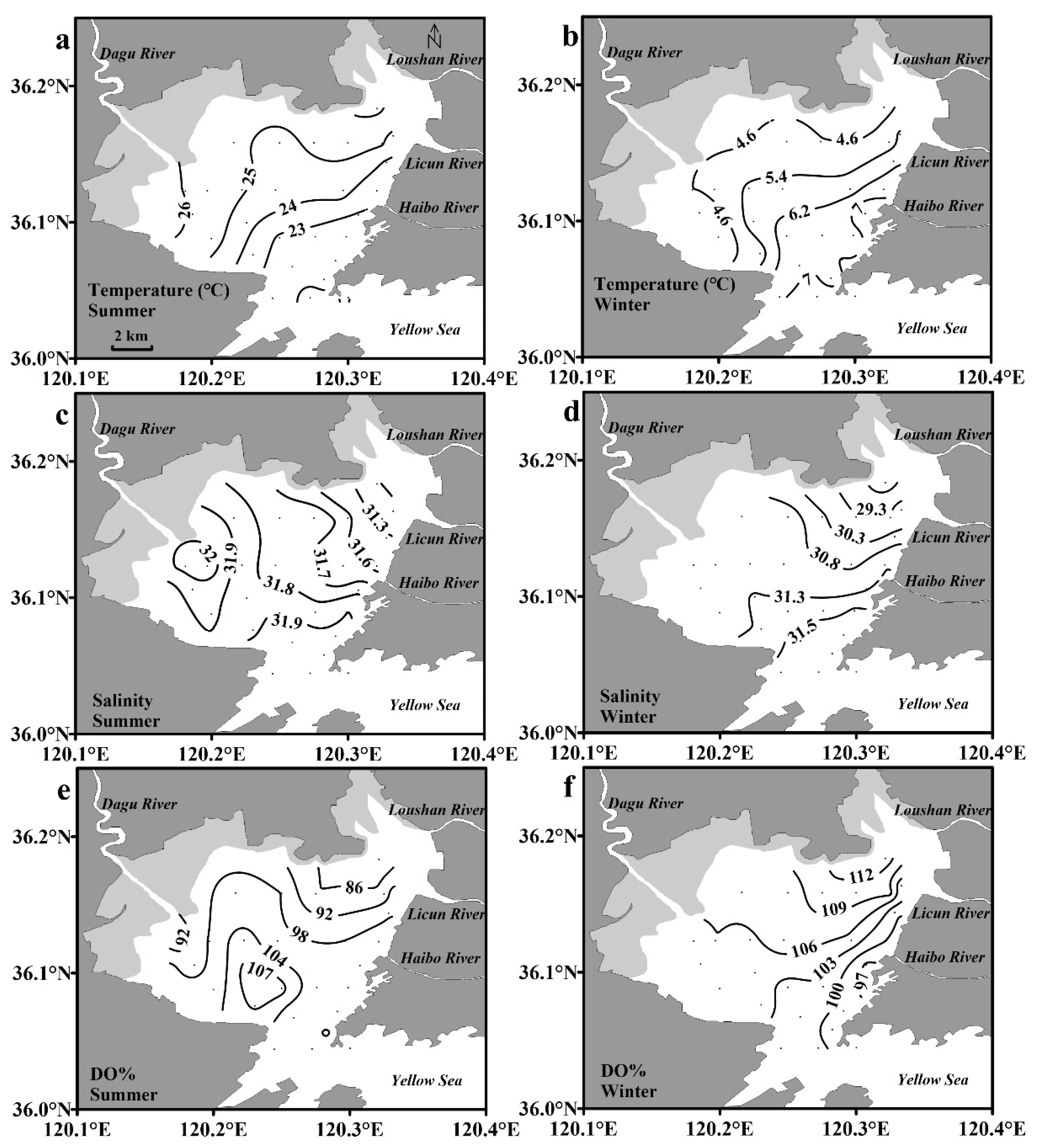
The seawater surface temperature was between 21.8 °C and 26.2 °C, with an average of 24.0 °C, in JZB during the summer, showing a decreasing trend from the upper end of the bay to the mouth of the bay. The highest temperature value appeared in the western area of the bay with the shallowest water depth. The temperature variation range in winter was 3.8~7.8 °C, and the average value was 5.8 °C. Due to the effects of land cooling, the temperature increased from the upper end of the bay to the mouth area, and the lowest value appeared in the western area. The ranges of seawater surface salinity were 31.0~32.1 in summer and 27.8~31.6 in winter, with average values of 31.8 and 30.9, respectively. The salinity variation gradient in winter was great and may have been related to the strong exchange of seawater between the Yellow Sea and the bay. In terms of distribution, the salinity showed an increasing trend from the northeastern area to the mouth area in the two periods. The salinity was the lowest and the gradient changed drastically in the northeastern area. Most of the rivers that enter JZB have no natural runoff at most of the time of a year and the estuaries have become conduits for wastewater discharge [27]. The total amount of wastewater treated by the three WWTPs located near the northeastern area of JZB is up to ~510,000 tons per day (Figure 1). Therefore, the direct input of treated wastewater was the main reason for the low salinity in this region [11,33]. Additionally, a high-salinity area with a value higher than 30.9 was found in the nearshore area of the western area in summer. Considering the shallow water depth (< 2 m) and the long water residence time (~100 d) in this region, it may be caused by strong evaporation. The range of seawater surface DO% was 81.1%~108.6% in summer, with an average of 98.7%. The DO values were unsaturated in the northeastern area and the area near the estuary of the Dagu River, while those in other areas were supersaturated. The lowest DO% value appeared in the northeastern area of the bay, and the highest value was observed in the southwestern area. The DO% values in winter were higher than those in summer, ranging from 96.5% to 113.8%, with an average of 103.9%. Except for the area near the estuary of the Haibo River, the DO in the entire bay was supersaturated, with the highest value (>110%) appearing in the northeastern area. In addition, the DO% distribution roughly showed a reverse pattern of the summer, and the DO% values decreased from the northeastern area to the mouth area (Figure 2).
3.2. Variations in Seawater Surface Ωarag, DIC and pH
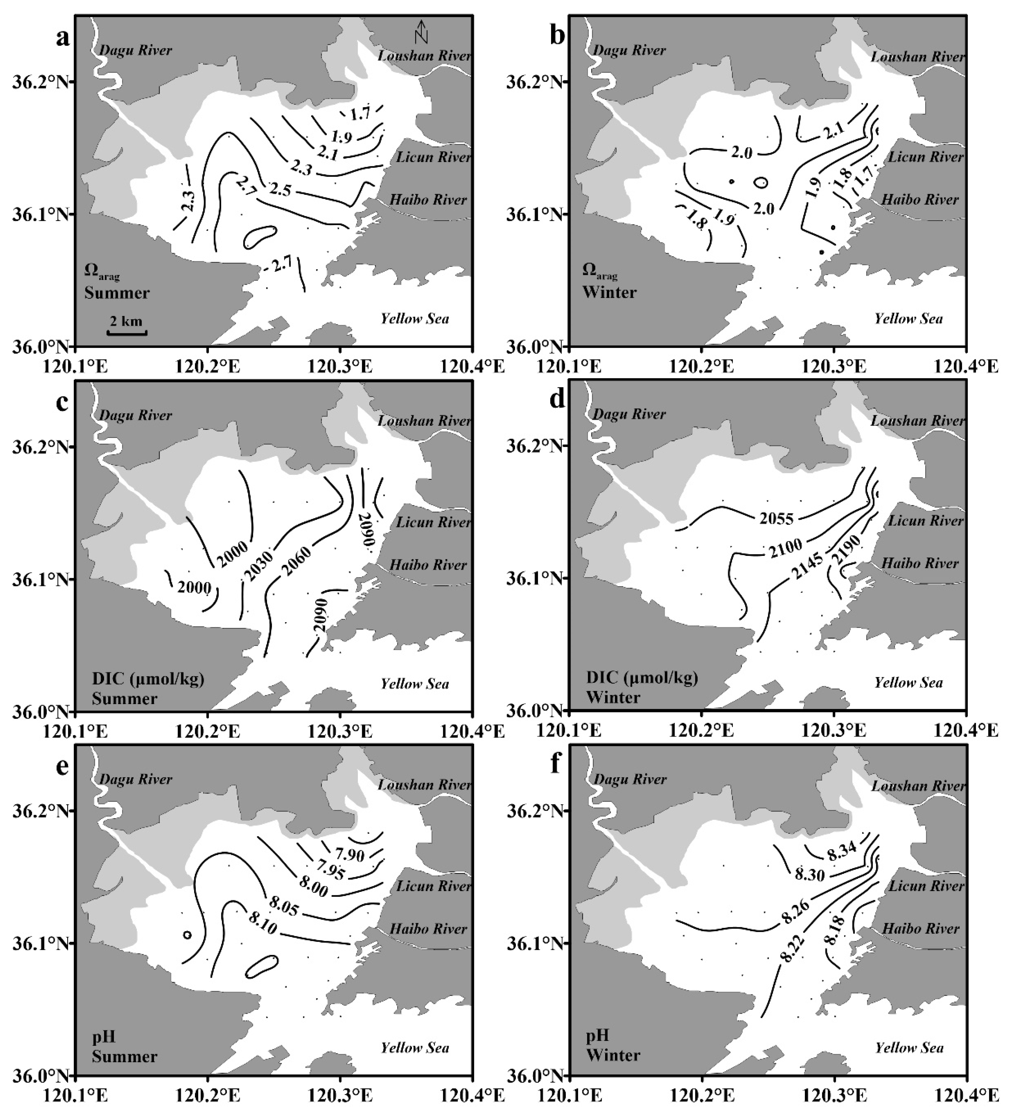
The seawater surface Ωarag was supersaturated in JZB during summer and winter. The Ωarag values in summer ranged from 1.55 to 2.92, with an average of 2.47, and the gradient variation was great. The lowest Ωarag value (< 2.10) was in the northeastern area, while values in most other areas exceeded 2.50, and the highest value (> 2.70) appeared in the nearshore area of the southwestern area. The Ωarag values in winter were between 1.62 and 2.15, with an average of 1.93. The Ωarag gradient variation in this period was obviously more gradual than that in summer, and the Ωarag value in most areas of JZB was approximately 1.90. The surface DIC ranged from 1979 μmol/kg to 2135 μmol/kg, with an average of 2057 μmol/kg, and the value showed a trend of increasing from the western area to the mouth area in summer. In winter, the DIC was in the range of 2027~2249 μmol/kg, with an average of 2122 μmol/kg, and generally increased from the northern area to the mouth area. The highest DIC value appeared in the area near the estuary of the Haibo River. The surface pH value ranged from 7.81 to 8.16, with an average of 8.06, and showed an increasing trend from the northeastern area to the mouth area in summer with high water temperature. In the winter with low water temperatures, the pH level was obviously higher, ranging from 8.12 to 8.37, with an average of 8.24. Moreover, the pH distribution trend was opposite that in summer and showed a trend of decreasing from the northeastern area to the mouth area (Figure 3).
3.3. Qualitative Identification of the Main Factors Controlling the Spatial Distribution of Surface Ωarag
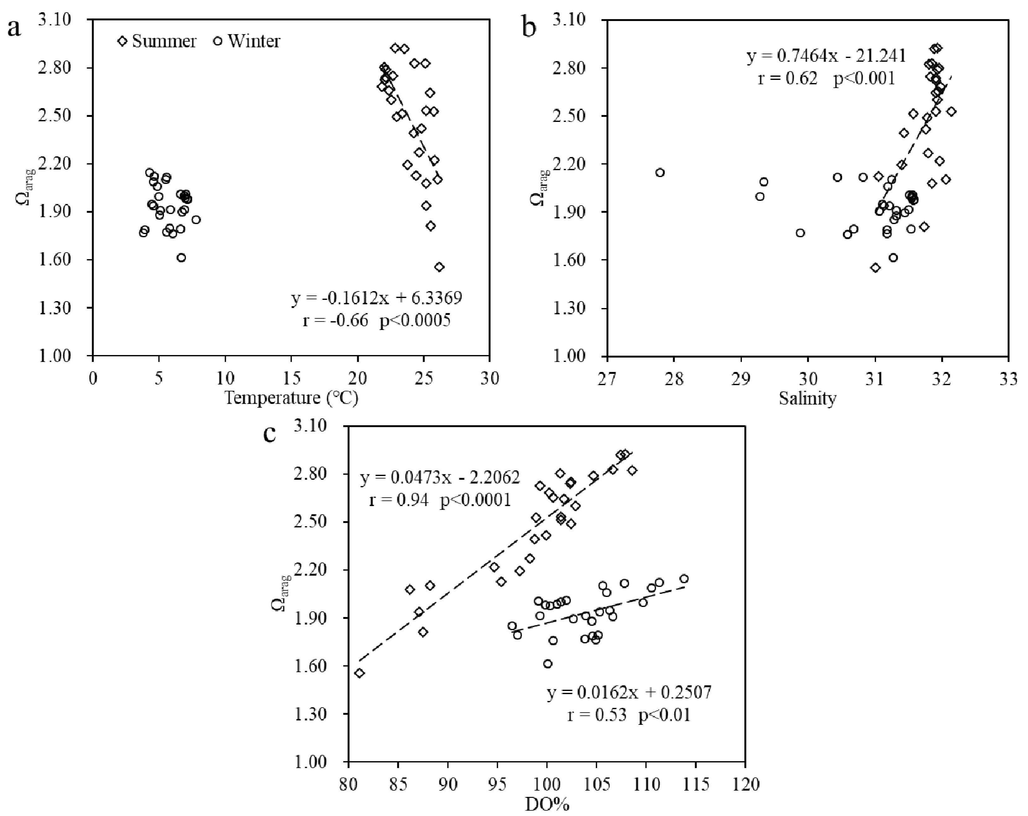
In coastal waters, seawater surface Ω is mainly controlled by temperature, mixing processes (mixing between terrestrial input and seawater) and biological processes [8,20,40,41]. The influence of temperature on Ω is mainly manifested in two aspects. On the one hand, without changing TA and DIC, an increase in seawater temperature can increase the first and second carbonic acid dissociation constants (k1 and k2) of carbonic acid and decrease the Ksp* of calcium carbonate [17,37], thereby promoting an increase in Ω. The difference between highest and lowest seawater temperatures for each investigated cruise were small: 4.4 °C in summer and 4.0 °C in winter. By normalizing the Ωarag of each station at in situ seawater temperatures to the average seawater temperature (24.01 °C for the summer and 5.76 °C for the winter) of the corresponding cruises, it is found that the change of Ωarag before and after the normalization was very small: ≤ 0.04 in summer and ≤ 0.02 in winter. The variation in difference between highest and lowest Ωarag values for each investigated cruise did not exceed 4% after normalization. This indicated that this process had little effect on the spatial distribution of Ωarag difference. On the other hand, an increase in seawater temperature can reduce the DIC level by reducing the solubility of CO2 in seawater without changing TA [42], thereby increasing Ω. Since the change in CO2 solubility in seawater often directly affects the CO2 exchange process at the sea-air interface, this effect is usually strong [20,41]. However, the Ωarag had no obvious correlation with seawater temperature in JZB during winter and a somewhat negative correlation in summer (Figure 4a). Obviously, temperature was not the main reason for the spatial distribution differences of Ωarag in these two cruises.
Terrestrial runoff usually has low pH and [CO32−] values, which directly lead to a decrease in Ωarag in the receiving water body [21,43]. The rivers entering JZB have no natural runoff, but the daily discharges of the Licun River WWTP, the Lushan River WWTP and the Haibo River WWTP, which are located at the three estuaries in the eastern area of the bay, are up to 250,000, 100,000 and 160,000 tons, respectively [11,44]. The direct input of treated wastewater has become the main form of terrestrial input, and unlike natural rivers affected by seasonal changes, treated wastewater input is a persistent process. The pH values of the treated wastewater from the three WWTPs were 7.16~7.33 in January and 7.44~7.50 in June [44]. The wastewater input with low pH values would directly reduce the Ωarag in the northeastern area of JZB. In summer, the Ωarag values in the northeastern area were just significantly lower than those in the central and mouth areas with high salinity values (Figure 3c). However, the Ωarag in the northeastern area was relatively high in winter, indicating that the effect of treated wastewater input was masked by other factors (Figure 3b).
Biological processes mainly include primary production and aerobic respiration. Primary production produces oxygen and consumes CO2, thus increasing Ωarag [45]. Conversely, aerobic respiration consumes oxygen and reduces Ωarag. During the summer, Ωarag had an excellent positive correlation with DO% (Figure 4c) (r = 0.94, p < 0.0001), suggesting that biological processes were the main factor affecting the distribution of Ωarag in JZB and might explain the main differences in the spatial distribution of Ωarag. According to the unsaturated DO levels, the dominance of aerobic respiration resulted in the lowest Ωarag in the northeastern area of JZB. However, in most other areas of JZB, the DO was supersaturated, and primary production was dominant, which led to higher Ωarag levels. During the winter, the oversaturated DO values in most areas of the entire bay meant that primary production was dominant, but the relationship between DO% and Ωarag only showed a relatively weaker negative correlation (Figure 4c) (r = 0.53, p < 0.01), indicating that the control of biological processes on the spatial distribution of Ωarag in winter was weaker than that in summer. Despite this, considering that Ωarag had no significant correlations with seawater temperature and salinity (Figure 4a,b), primary production may still be the main factor affecting the Ωarag distribution in winter, and the weak negative correlation between DO% and Ωarag may be the result of the effects of the mixing processes and regional temperature variation. For example, treated wastewater input with low pH values could decrease the Ωarag levels in the northeastern area where the DO% (> 107%) values were highest, the low seawater temperature could cause a decrease in Ωarag in the western area where the DO% values were approximately 105%, and the strong external seawater exchange could cause an increase in Ωarag in the mouth area where the DO% values were near 100% (Figure 2b,f and Figure 3b).
The regression analysis indicates that biological processes may be the main factor affecting the spatial difference of Ωarag in JZB during summer and winter, while the influence of temperature and mixing processes is relatively smaller. However, the specific contributions of the above three processes could not be calculated if only using the regression analysis, and the correlation between parameters may even obscure the important role of certain processes in some cases. For example, direct input of the treated wastewater had the most significant impact in the northeastern area with the lowest DO% values and the strongest degradation of organic matter during summer, and the excellent positive correlation between Ωarag and DO% (Figure 4c) partly included the contribution of the treated wastewater input. Therefore, a further quantification analysis involving the contributions of the above three processes to the spatial distribution of Ωarag is still necessary.
3.4. Processes Controlling the Spatial Distribution of Surface Ωarag Revealed by Quantitative Evaluation
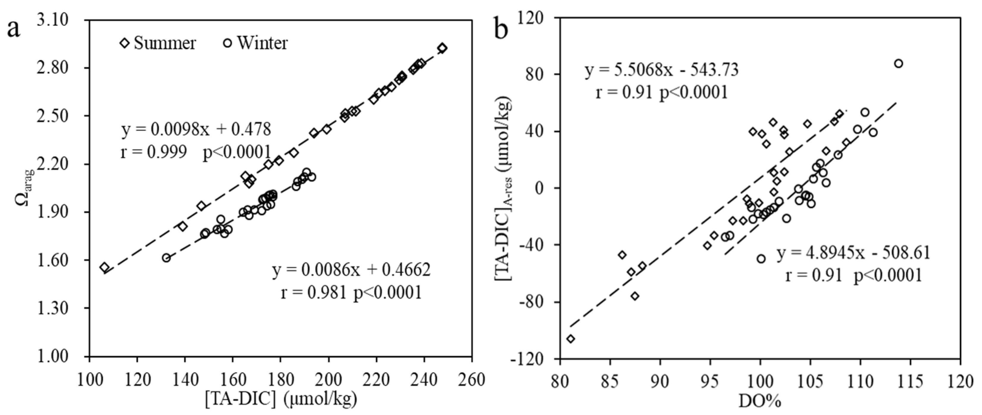
In the carbonate system, the change in Ωarag with salinity is nonlinear and non-conservative, so Ωarag is not convenient for quantitative calculations. The Ωarag in seawater is essentially determined by the [CO32−] value, and the difference between TA and DIC ([TA-DIC]) can reflect the levels of [CO32−] well, thereby acting as a good proxy for Ωarag [20,46]. As shown in Figure 5a, a significant positive correlation (with r values close to 1) was observed between Ωarag and [TA-DIC] in JZB in both summer and winter. Thus, the effects of the temperature, mixing processes and biological processes on Ωarag could be converted to [TA-DIC]. To quantify the contribution of each factor to [TA-DIC], the [TA-DIC] and salinity of each station were subtracted from the average [TA-DIC] and salinity values of the corresponding cruises, and then [TA-DIC]A and SA were obtained. Accordingly, the above evaluation problem was transformed into the calculation of the contribution to [TA-DIC]A from temperature variation, the mixing processes and biological processes.
For the contribution of temperature variation, only the effect of temperature on the solubility of CO2 in seawater was evaluated in these two cruises, due to the negligible Ωarag changes caused by the variation of k1 and k2 of carbonic acid and Ksp* of calcium carbonate from temperature (Section 3.3). In the calculation process, taking the average TA and salinity of the cruise as the staring values (the average TA and salinity were 2260.1 μmol/kg and 31.76 in summer and 2291.4 μmol/kg and 30.93 in winter, respectively) and assuming seawater CO2 reached equilibrium with the atmosphere at in situ temperature of each station, this research calculated the corresponding DIC (DICeq) of each station at different temperatures and the DIC (DICavg) at the average temperature of the corresponding cruise at this equilibrium state using the CO2SYS program [36]. Then, the difference between DICavg and DICeq was the contribution from the temperature of the corresponding station to [TA-DIC]A ([TA-DIC]A-tem) (Equation (1)).
where the DICeq and DICavg are the DIC value at in situ temperature of the station and at the average temperature of the corresponding cruise, respectively, when seawater CO2 reached equilibrium with the atmosphere. Atmospheric CO2 concentration data from flask measurements in the Tae-ahn Peninsula (126.13° E, 36.73° N) adjacent to the southern Yellow Sea were used, with values of 410 μatm in January 2017 and 395 μatm in June 2017, respectively (ftp://ftp.cmdl.noaa.gov/data/greenhouse_gases/co2/flask).
[TA-DIC]A-tem = DICavg − DICeq
For the contribution of the mixing processes to [TA-DIC]A, considering that the direct input of treated wastewater is the main form of terrestrial input, this study used the [TA-DIC] values of the treated wastewater and the station in the mouth area of the bay with the highest salinity as the freshwater and seawater end-member, respectively. Thus, the change ratio of [TA-DIC] per unit salinity was obtained. The [TA-DIC] values of the treated wastewater were obtained from Liu et al. [44], and the [TA-DIC] value of the freshwater end-member was calculated according to the proportion of three WWTPs’ discharge (∑([TA-DIC]I × Qi)/∑Qi, Q was the charge, Table 1). The freshwater end-member values were −405 μmol/kg in January and −110 μmol/kg in June. The seawater end-member set to the L2 station, which was closest to the Yellow Sea, and the [TA-DIC] and salinity values were 173 μmol/kg and 31.6 in January and 236 μmol/kg and 32.0 in June, respectively. Then, the contribution of the mixing processes to the [TA-DIC]A ([TA-DIC]A-mix) were calculated by multiplying by SA (Equation (2)).
where the [TA-DIC]tw and [TA-DIC]sea are the [TA-DIC] values of the treated wastewater and seawater end-member, respectively; Ssea is the salinity of the seawater end-member. SA is the difference between salinity of station and average salinity of the corresponding cruise.
[TA-DIC]A-mix = ([TA-DIC]tw − [TA-DIC]sea)/(−Ssea) × SA
Meanwhile, compared with seawater, the treated wastewater had different temperatures, indicating that mixing term may include some bias from temperature changes. Temperature mixes linearly, so this component can be estimated if the proportion of treated wastewater in seawater can be obtained. According to mass balance, the sample salinity of a station can be calculated as follows [11]:
where y is the proportion of wastewater in seawater and Si is the salinity of the station i.
Si = Ssea/(1 + y)
In January and June, the lowest salinity value in the eastern area of the bay was 27.8 and 31.0, respectively. According to the Equation (3), the y values were calculated as 0.13 and 0.03, respectively. The temperature difference between treated wastewater and seawater in the eastern area did not exceed 7.6 °C in January and 4.5 °C in June, indicating that the temperature changes caused by this mixing process were ≤ 1.0 °C in January and ≤ 0.14 °C in June. Therefore, the effect of this process on Ωarag could be ignored in the current study.
The [TA-DIC]A value after the deduction of the effects from temperature and mixing processes was the contribution of other processes ([TA-DIC]A-res) (Equation (4)).
where the [TA-DIC]A-tem and [TA-DIC]A-mix are the contribution of temperature and mixing processes to the [TA-DIC]A, respectively.
[TA-DIC]A-res = [TA-DIC]A − [TA-DIC]A-tem − [TA-DIC]A-mix
After stripping off the effects of temperature and mixing processes, [TA-DIC]A-res showed an excellent positive correlation with DO% (r = 0.91, p < 0.0001), indicating that [TA-DIC]A-res basically reflected the contribution of biological processes to [TA-DIC]A. This further verified the rationality of this estimation method. Thus, the relative contribution percentage of the three processes to [TA-DIC]A were evaluated.
The relative contributions of each process to [TA-DIC]A in summer are shown in Figure 6. The relative contribution of temperature to [TA-DIC]A was the largest in the northwestern area of the bay with the highest seawater temperature, exceeding 45%. However, in other areas, it was smaller, less than 30%. The mixing processes had the minimum relative contribution, and most of the regions featured values of less than 10%; however, the contribution reached 13% in the northeastern area, which had the strongest impact of treated wastewater input. The biological processes had the maximum relative contribution to [TA-DIC]A, which was more than 50% in most regions. In the northeastern area with the lowest DO% (<90%) and the southwestern area with the highest DO% (>105%), the relative contribution of biological processes exceeded 85%. Overall, the average contributions of temperature, mixing processes and biological processes to [TA-DIC]A were 25%, 5% and 70%, respectively. The biological processes were the main factor controlling the spatial distribution of Ωarag in JZB during summer. It is worth noting that the effects of temperature and mixing processes on [TA-DIC]A were mutually reinforced with biological processes in most areas in this period. In the northeastern area with the minimum value of Ωarag, the main effect was that treated wastewater input and aerobic respiration together caused the reduction of [TA-DIC]A, and the contributions of the two were up to 90%. In the southwestern area with the maximum value of Ωarag, primary production and the higher seawater temperature lead to an increase in [TA-DIC]A, and the combined contributions of the two reached approximately 90%. As such, there were marked difference in Ωarag among the various regions of JZB in summer.
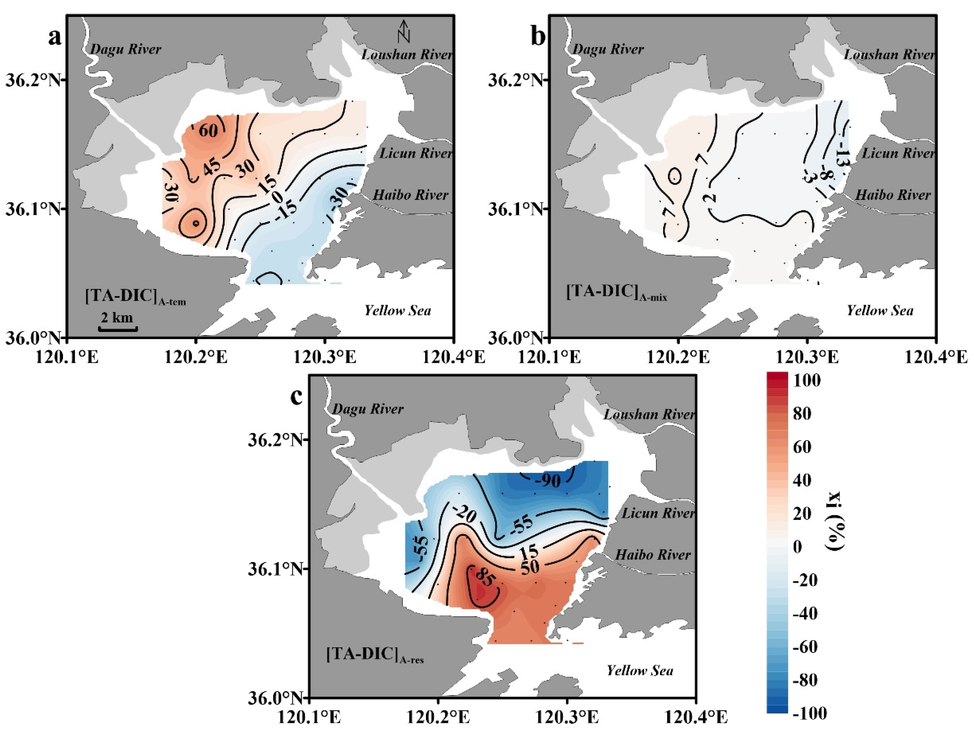
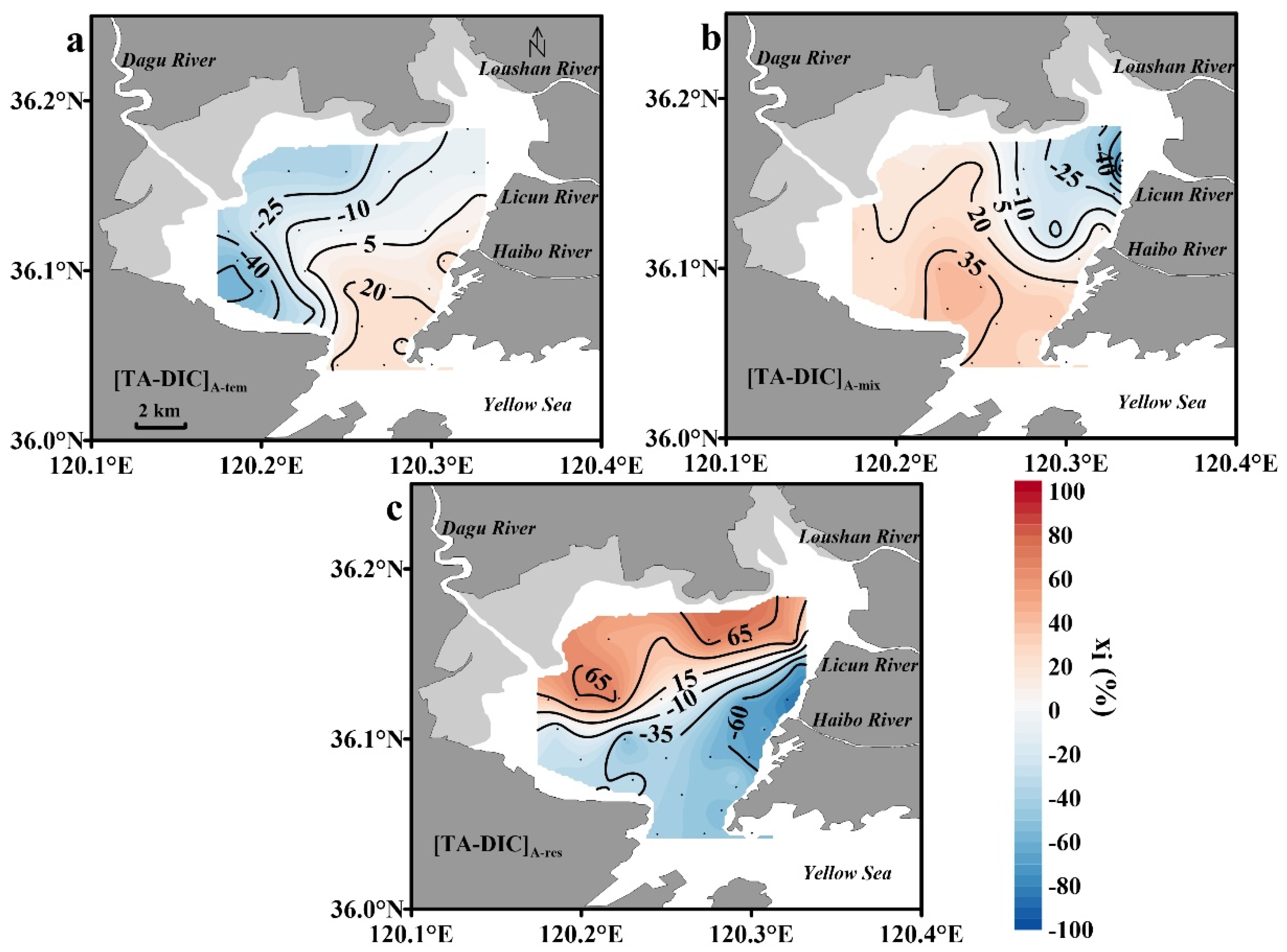
In winter (Figure 7), the relative contribution of temperature to [TA-DIC]A was largest and exceeded 45% in the western area where the seawater temperature was lowest; in the other regions, the contribution was less, below 25%. The relative contribution of the mixing processes to [TA-DIC]A was much higher in winter than in summer and was more than 30% in the northeastern area with the lowest salinity (<30.0) and the mouth area with the highest salinity (>31.5). This may be related to enhanced exchange of seawater between the bay and the Yellow Sea caused by the low seawater temperatures and high wind speeds in winter. The biological processes contributed the most to [TA-DIC]A, and the relative contribution was more than 60% in the northern area and the area near the estuary of the Haibo River. During this period, DO values in most areas of the entire bay were supersaturated, and primary production was dominant, which corresponds to the growth peak of phytoplankton in JZB in winter [25,26,27]. Overall, the average relative contributions of temperature, mixing processes and biological processes to [TA-DIC]A were 20%, 30% and 50%, respectively. The biological processes were also the main processes contributing to spatial differences in Ωarag in winter in JZB, but the total contribution of temperature and mixing processes was similar to that of the biological processes in this period. Furthermore, different from the situation in summer, the effects of the above three processes on [TA-DIC]A showed mutual cancellation in most areas. In the northeastern area where DO% values exceeded 109%, the low seawater temperature and treated wastewater input had a negative effect on [TA-DIC]A, while the strong primary production had a positive effect on [TA-DIC]A, resulting in a net increase in [TA-DIC]A of only approximately 10%. In the western area, the relative contribution of the mixing processes and primary production, corresponding to an increase in [TA-DIC]A, was approximately 60%, whereas the remaining 40% contribution corresponded to a decrease in [TA-DIC]A caused by low seawater temperatures. Therefore, the differences in Ωarag among the various regions in JZB were markedly reduced in winter.
In the open ocean, physical transport in the horizontal and vertical directions is a key factor causing differences in the distribution of Ω [47,48,49], while the increasing human disturbance has affected the biological processes more prominently in coastal waters. In ocean shelf regions, the effect of biological processes on Ω mainly appears in the summer. Due to the stratification of seawater, the surface water body often features strong primary production, which increases Ω under the appropriate illumination and nutrient supply conditions, while organic matter deposited from the upper water body often leads to strong aerobic respiration in the subsurface water body, resulting in low Ω and pH [8,50,51]. However, in nearshore bays where the impact of human activities is more significant, the situation is slightly different. The urbanization process affects biological processes in certain areas. For example, in the JZB, the eastern area of the bay, which is adjacent to downtown Qingdao, receives large amounts of terrestrial pollutants brought by wastewater all the year round and is dominated by aerobic respiration. This situation can weaken the living environment of calcified organisms in the region and does not change even after heavy rain [33,35]. In contrast, in the western area, which is far from the urban area and adjacent to the wetland, primary production produces an increase in Ω, and this region is an important area for shellfish farming in JZB [52]. A similar phenomenon was also observed in Fujian, Southeast China [53,54] and Guanabara Bay in Brazil [25]. Moreover, perennial eutrophication often causes algal blooms and produces strong primary production even under the low temperatures in winter in some waterbodies [55,56], offsetting the decrease in Ω caused by the low temperatures. In addition, bays often have a shallow water depth, and strong turbulence might cause full mixing of the seawater vertically, making the effect of biological activity on Ω extend through the entire water column [23]. With the rapid urbanization and worsening climate change in coastal areas, the effects of strong heterotrophic bacteria activity and vigorous plankton growth on Ω will become increasingly prominent. Thankfully, environmental protection has been received increasing attention in China. Central and local governments have accelerated efforts to tackle environmental pollution by raising environmental protection standards and revising laws [57,58]. However, strict enforcement of environmental protection laws is urgently needed to conserve the aquatic environment, particularly the effective treatment of wastewater which brought large amounts of organic matters and nutrients to coastal environment [59]. In the future, collaboration between government, industry and environmental non-governmental organizations (NGO) will be of great importance to mitigate ocean acidification and other problems in coastal areas.
3.5. Uncertainty Analysis of the Quantitative Estimate
Here the uncertainty associated with key terms in the quantitative evaluation method in Section 3.4 was analysed. First, the uncertainty of TA and Ωarag calculated from the pH and DIC were estimated to be ~7 μmol/kg and ~0.05, respectively, via the CO2SYS program (without considering the uncertainty induced by carbonate acid dissociation constants during calculations) [60], given the uncertainty of ~2 μmol/kg for DIC and the uncertainty of 0.01 for pH measurement. The TA uncertainty will lead to an uncertainty of ~7.3 μmol/kg, or (72 + 22)0.5, for [TA-DIC]. This uncertainty will propagate into [TA-DIC]A (~7.4 μmol/kg, or (7.32 + 7.32/28) 0.5), Xi-tem and Xi-mix (< 5.5%) and Xi-res (< 8%). Second, [TA–DIC] has some limitations as a proxy for in situ Ωarag. In the current study, [TA-DIC] may not accurately reflect the influence of temperature. The effect of temperature only refers to its impact on thermodynamic constants or internal allocation of carbonate system species by temperature driven acid-base equilibrium under conditions of constant TA and DIC, which is called “internal temperature effect” [20]. For instance, for one unit increase in temperature, Ωarag will increase by ~0.60% °C−1 based on our data. Fortunately, the thermal influence is relatively minor due to the small spatial variation in seawater temperature for each investigated cruise. Meanwhile, to calculate the effects of temperature on the solubility of CO2 in seawater, it is assumed that seawater pCO2 can reach an equilibrium state with the atmospheric CO2 quickly. In fact, it is almost impossible to reach transient air-sea CO2 equilibrium due to the slow air-sea CO2 exchange [61], which will lead to overestimation or underestimation of DICeq. However, this influence on [TA-DIC]A-tem may be minor since this overestimated or underestimated part offset, to a large extent, each other after subtraction as shown from Equation (1). Third, to separate mixing effects, the slope values of [TA-DIC]-Salinity between the composite treated wastewater and seawater in January and June were estimated from end-members values. Treated wastewater end-member values were calculated by the [TA-DIC] values and discharge of three WWTPs in corresponding months which were reported by Liu et al. [44]. Though their studies showed that changes in DIC and TA were generally same in the two years, the uncertainties brought by the treated wastewater end-member in our cruises still exist in [TA-DIC]A-mix. Despite some uncertainties in our methods which are also widely applied in other studies, the current study provides some quantitative findings on the control mechanism of Ωarag in the bays under the influence of human activities.
3.6. Limitation and Future Research
Similar to many studies, some limitations exist in the current research. First, Ωarag and TA were calculated based on pH and DIC. The uncertainty of pH measurements made with electrodes calibrated on the NBS scale may cause a certain level of inaccuracy [62,63]. Thankfully, the spatiotemporal changes of pH in JZB were large enough, and the conclusions were valid based on these data. Second, this study focused the contributions of three factors (temperature, biological processes and mixing processes) to the distribution of Ωarag. However, the effects of other factors, for example, mineral precipitation, vertical mixing of water column, nitrification processes, may also exist, although their contributions may be minor in our research area. Additionally, the effects of urbanization on Ωarag include sewage input and other factors. Third, the seasonal changes of Ωarag is unavailable due to the data limitation. Obviously, more cruise investigations and related studies are still needed to improve our understanding of the complex ocean acidification under the impact of climate change and human activities.
4. Conclusions
Seawater surface aragonite saturation state (Ωarag) during summer and winter in Jiaozhou Bay, China, was analysed in this study. The seawater surface Ωarag was supersaturated, and the ranges were 1.55~2.92 in summer and 1.62~2.15 in winter, respectively. In addition to the analysis of the effects of temperature, mixing processes and biological processes on the spatial difference of Ωarag based on regression analysis with surface temperature, salinity and DO%, the relative contributions of these three processes were quantified by introducing the difference between TA and DIC as a proxy for Ωarag. The results showed that the biological processes were the main processes affecting the spatial difference of Ωarag, and the relative contribution was 70% in summer and 50% in winter. The contributions of temperature (25% in summer and 20% in winter) and mixing processes (5% in summer and 30% in winter) were smaller. Moreover, the interaction among the three factors that influence Ωarag exhibited mutual promotion in summer and mutual cancellation in winter, causing the regional distribution of Ωarag to show marked difference in summer and a relatively uniform change in winter.
Author Contributions
Conceptualization, L.Z. and Y.L.; methodology, software, validation and writing—original draft preparation, Y.L., L.X., L.Z. and H.Y.; investigation and formal analysis, L.X. and Y.L.; writing—review and editing, L.Z., Y.L. and H.Y.; supervision, Y.L., W.F. and F.L. All authors have read and agreed to the published version of the manuscript.
Funding
This research was funded by the National Natural Science Foundation of China, grant number 41376123, the Excellent Doctors Come to Shanxi to Reward Scientific Research Projects, grant number SXYBKY2018020 and the Science and Technology Foundation of Shanxi Agricultural University, China, grant number 2018YJ21.
Conflicts of Interest
The authors declare no conflict of interest.
References
- Cooley, S.R.; Doney, S.C. Anticipating ocean acidification’s economic consequences for commercial fisheries. Environ. Res. Lett. 2009, 4, 24007. [Google Scholar] [CrossRef]
- Carter, B.R.; Toggweiler, J.R.; Key, R.M.; Sarmiento, J.L. Processes determining the marine alkalinity and calcium carbonate saturation state distributions. Biogeosciences 2014, 11, 7349–7362. [Google Scholar] [CrossRef] [Green Version]
- Xu, D.; Wang, D.; Li, B.; Fan, X.; Zhang, X.W.; Ye, N.H.; Wang, Y.; Mou, S.; Zhuang, Z. Effects of CO2 and Seawater Acidification on the Early Stages of Saccharina japonica Development. Environ. Sci. Technol. 2015, 49, 3548–3556. [Google Scholar] [CrossRef] [PubMed]
- Albright, R.; Takeshita, Y.; Koweek, D.A.; Ninokawa, A.; Wolfe, K.; Rivlin, T.; Nebuchina, Y.; Young, J.; Caldeira, K. Carbon dioxide addition to coral reef waters suppresses net community calcification. Nature 2018, 555, 516–519. [Google Scholar] [CrossRef] [PubMed]
- Zhai, W.D.; Zheng, N.; Huo, C.; Xu, Y.; Zhao, H.D.; Li, Y.W.; Zang, K.P.; Wang, J.Y.; Xu, X.M. Subsurface pH and carbonate saturation state of aragonite on the Chinese side of the North Yellow Sea: Seasonal variations and controls. Biogeosciences 2014, 11, 1103–1123. [Google Scholar] [CrossRef] [Green Version]
- Mathis, J.T.; Cooley, S.R.; Lucey, N.; Colt, S.; Ekstrom, J.; Hurst, T.; Hauri, C.; Evans, W.; Cross, J.N.; Feely, R.A. Ocean acidification risk assessment for Alaska’s fishery sector. Progess Oceanogr. 2015, 136, 71–91. [Google Scholar] [CrossRef] [Green Version]
- Yang, P.; Zhang, Y.; Yang, H.; Zhang, Y.; Xu, J.; Tan, L.; Tong, C.; Lai, D.Y.F. Large Fine-Scale Spatiotemporal Variations of CH4 Diffusive Fluxes From Shrimp Aquaculture Ponds Affected by Organic Matter Supply and Aeration in Southeast China. J. Geophys. Res. 2019, 124, 1290–1307. [Google Scholar] [CrossRef]
- Cai, W.; Hu, X.; Huang, W.; Murrell, M.C.; Lehrter, J.C.; Lohrenz, S.E.; Chou, W.; Zhai, W.; Hollibaugh, J.T.; Wang, Y.; et al. Acidification of subsurface coastal waters enhanced by eutrophication. Nat. Geosci. 2011, 4, 766–770. [Google Scholar] [CrossRef]
- Mathis, J.T.; Cross, J.N.; Bates, N.R. Coupling primary production and terrestrial runoff to ocean acidification and carbonate mineral suppression in the eastern Bering Sea. J. Geophys. Res. 2011, 116, C2030. [Google Scholar] [CrossRef]
- Xue, L.; Wang, H.; Jiang, L.; Cai, W.; Wei, Q.; Song, H.; Kuswardani, R.T.D.; Pranowo, W.S.; Beck, B.; Liu, L.; et al. Aragonite saturation state in a monsoonal upwelling system off Java, Indonesia. J. Mar. Syst. 2016, 153, 10–17. [Google Scholar] [CrossRef]
- Yang, X.; Xue, L.; Li, Y.; Han, P.; Liu, X.; Zhang, L.; Cai, W.J. Treated Wastewater Changes the Export of Dissolved Inorganic Carbon and Its Isotopic Composition and Leads to Acidification in Coastal Oceans. Environ. Sci. Technol. 2018, 52, 5590–5599. [Google Scholar] [CrossRef] [PubMed]
- Riebesell, U. Effects of CO2 enrichment on marine phytoplankton. J. Oceanogr. 2004, 60, 719–729. [Google Scholar] [CrossRef]
- Waldbusser, G.G.; Hales, B.; Langdon, C.J.; Haley, B.A.; Schrader, P.; Brunner, E.L.; Gray, M.W.; Miller, C.A.; Gimenez, I. Saturation-state sensitivity of marine bivalve larvae to ocean acidification. Nat. Clim. Chang. 2015, 5, 273–280. [Google Scholar] [CrossRef]
- Feely, R.A.; Byrne, R.H.; Acker, J.G.; Betzer, P.R.; Chen, C.A.; Gendron, J.F.; Lamb, M.F. Winter-summer variations of calcite and aragonite saturation in the Northeast Pacific. Mar. Chem. 1988, 25, 227–241. [Google Scholar] [CrossRef]
- Doney, S.C.; Fabry, V.J.; Feely, R.A.; Kleypas, J.A. Ocean Acidification: The Other CO2 Problem. Annu. Rev. Mar. Sci. 2009, 1, 169–192. [Google Scholar] [CrossRef] [Green Version]
- Gruber, N.; Hauri, C.; Lachkar, Z.; Loher, D.; Frã Licher, T.L.; Plattner, G.K. Rapid progression of ocean acidification in the California Current System. Science 2012, 337, 220–223. [Google Scholar] [CrossRef] [Green Version]
- Mucci, A. The solubility of calcite and aragonite in seawater at various salinities, temperature, and one atmosphere total pressure. Am. J. Sci. 1983, 238, 780–799. [Google Scholar] [CrossRef]
- Morse, J.W.; Arvidson, R.S.; Luttge, A. Calcium carbonate formation and dissolution. Chem. Rev. 2007, 107, 342–381. [Google Scholar] [CrossRef]
- Harris, K.E.; DeGrandpre, M.D.; Hales, B. Aragonite saturation state dynamics in a coastal upwelling zone. Geophys. Res. Lett. 2013, 40, 2720–2725. [Google Scholar] [CrossRef]
- Xue, L.; Cai, W.; Sutton, A.J.; Sabine, C. Sea surface aragonite saturation state variations and control mechanisms at the Gray’s Reef time-series site off Georgia, USA (2006–2007). Mar. Chem. 2017, 195, 27–40. [Google Scholar] [CrossRef]
- Zhai, W.; Zang, K.; Huo, C.; Zheng, N.; Xu, X. Occurrence of aragonite corrosive water in the North Yellow Sea, near the Yalu River estuary, during a summer flood. Estuar. Costal Shelf Res. 2015, 166, 199–208. [Google Scholar] [CrossRef]
- Kim, D.; Park, G.H.; Baek, S.H.; Choi, Y.; Kim, T.W. Physical and biological control of aragonite saturation in the coastal waters of southern South Korea under the influence of freshwater. Mar. Pollut. Bull. 2018, 129, 318–328. [Google Scholar] [CrossRef] [PubMed]
- Kim, D.; Choi, S.; Yang, E.; Kim, K.; Jeong, J.; Kim, Y.O. Biologically Mediated Seasonality of Aragonite Saturation States in Jinhae Bay, Korea. J. Coast. Res. 2013, 29, 1420–1426. [Google Scholar]
- Yamamoto-Kawai, M.; Kawamura, N.; Ono, T.; Kosugi, N.; Kubo, A.; Ishii, M.; Kanda, J. Calcium carbonate saturation and ocean acidification in Tokyo Bay, Japan. J. Oceanogr. 2015, 71, 427–439. [Google Scholar] [CrossRef]
- Cotovicz, L.C.; Knoppers, B.A.; Brandini, N.; Poirier, D.; Costa Santos, S.J.; Abril, G. Aragonite saturation state in a tropical coastal embayment dominated by phytoplankton blooms (Guanabara Bay—Brazil). Mar. Pollut. Bull. 2018, 129, 729–739. [Google Scholar] [CrossRef]
- Liu, S.M.; Zhang, J.; Chen, H.T.; Zhang, G.S. Factors influencing nutrient dynamics in the eutrophic Jiaozhou Bay, North China. Prog. Oceanogr. 2005, 66, 66–85. [Google Scholar] [CrossRef]
- Gao, Z.; Yang, D.; Qin, J.; Xiang, L.; Zhang, K. The land-sourced pollution in the Jiaozhou Bay. Chin. J. Oceanol. Limnol. 2008, 26, 229–232. [Google Scholar] [CrossRef]
- Wu, Y.; Sun, S.; Zhang, Y.; Zhang, F. Quantitative study in long-term variation of phytoplankton in Jiaozhou Bay. Oceanol. Et Limnol. Sin. 2004, 35, 518–523. (In Chinese) [Google Scholar]
- Sun, X.X.; Sun, S.; Zhang, Y.S.; Zhang, F. Long-term changes of chlorophyll a concentration and primary productivity in the Jiaozhou Bay. Oceanol. Et Limnol. Sin. 2011, 5, 654–661. (In Chinese) [Google Scholar]
- Wang, Y.; Zhe, L.; Yong, Z.; Min, W.; Liu, D. Temporal and spatial variations of chlorophyll a and environmental factors in Jiaozhou Bay in 2010–2011. Acta Oceanol. Sin. 2015, 37, 103–116. (In Chinese) [Google Scholar]
- Weihua, Y.; Huiwang, G.; Hongying, L.; Yonggang, G.; Mingzhu, F. Preliminary study on effects of scallop cultivation on water quality in Jiaozhou Bay. Trans. Oceanol. Limnol. 2007, 2, 86–93. (In Chinese) [Google Scholar]
- Zhang, L.; Xue, M.; Liu, Q. Distribution and seasonal variation in the partial pressure of CO2 during autumn and winter in Jiaozhou Bay, a region of high urbanization. Mar. Pollut. Bull. 2012, 64, 56–65. [Google Scholar] [CrossRef] [PubMed]
- Li, Y.; Yang, X.; Ping, H.; Liang, X.; Zhang, L. Controlling mechanisms of surface partial pressure of CO2 in Jiaozhou Bay during summer and the influence of heavy rain. J. Mar. Syst. 2017, 173, 49–59. [Google Scholar] [CrossRef]
- Chen, C.; Ji, R.; Zheng, L.; Zhu, M.; Rawson, M. Influences of physical processes on the ecosystem in Jiaozhou Bay: A coupled physical and biological model experiment. J. Geophys. Res. 1999, 104, 29925–29949. [Google Scholar] [CrossRef]
- Liu, X.; Yang, X.; Li, Y.; Zhang, L. Sea surface pCO2 in an urbanized coastal system (Jiaozhou Bay, China) during summer. Mar. Pollut. Bull. 2019, 146, 767–778. [Google Scholar] [CrossRef]
- Lewis, E.; Wallace, D.W.R. Program developed for CO2 systems calculations. In ORNL/CDIAC 105; Carbon Dioxide Information Analysis Center, Oak Ridge National Laboratory US Department of Energy: Oak Ridge, TN, USA, 1998. [Google Scholar]
- Mehrbach, C. Measurement of the apparent dissociation constants of carbonic acid in seawater at atmospheric pressure. Limnol. Oceanogr. 1973, 18, 897–907. [Google Scholar] [CrossRef]
- Dickson, A.G.; Millero, F.J. A comparison of the equilibrium constants for the dissociation of carbonic acid in seawater media. Deep Sea Res. Part A Oceanogr. Res. Pap. 1987, 34, 1733–1743. [Google Scholar] [CrossRef]
- Millero, F.J. The thermodynamics of the carbonate system in seawater. Geochim. Cosmochim. Acta 1979, 43, 1651–1661. [Google Scholar] [CrossRef]
- Toledano, A.; Álvarez, M.I.; Solé, M.; Martínez Nadal, J.; Murcia Sáiz, A.; Parra, N.D. Controls on the seasonal variability of calcium carbonate saturation states in the Atlantic gateway to the Arctic Ocean. Mar. Chem. 2014, 158, 1–9. [Google Scholar]
- Jiang, L.Q.; Feely, R.A.; Carter, B.R.; Greeley, D.J.; Arzayus, K.M. Climatological distribution of aragonite saturation state in the global oceans. Glob. Biogeochem. Cycles 2015, 29, 1656–1673. [Google Scholar] [CrossRef]
- Weiss, R.F. Carbon dioxide in water and seawater: The solubility of a non-ideal gas. Mar. Chem. 1974, 2, 203–215. [Google Scholar] [CrossRef]
- Cao, Z.; Dai, M.; Zheng, N.; Wang, D.; Li, Q.; Zhai, W.; Meng, F.; Gan, J. Dynamics of the carbonate system in a large continental shelf system under the influence of both a river plume and coastal upwelling. J. Geophys. Res. 2011, 116, G2010. [Google Scholar] [CrossRef] [Green Version]
- Liu, X.Y.; Yang, X.F.; Li, Y.X.; Zang, H.; Zhang, L.J. Variations in dissolved inorganic carbon species in effluents from large-scale municipal wastewater treatment plants (Qingdao, China) and their potential impacts on coastal acidification. Environ. Sci. Pollut. Res. 2019, 26, 15019–15027. [Google Scholar] [CrossRef] [PubMed]
- Redfield, A.C. The influence of organisms on the composition of seawater. Sea 1963, 2, 26–77. [Google Scholar]
- Xue, L.; Cai, W.; Takahashi, T.; Gao, L.; Wanninkhof, R.; Wei, M.; Li, K.; Feng, L.; Yu, W. Climatic modulation of surface acidification rates through summertime wind forcing in the Southern Ocean. Nat. Commun. 2018, 9, 1–11. [Google Scholar] [CrossRef]
- Kuchinke, M.; Tilbrook, B.; Lenton, A. Seasonal variability of aragonite saturation state in the Western Pacific. Mar. Chem. 2014, 161, 1–13. [Google Scholar] [CrossRef]
- Kim, T.; Park, G.; Kim, D.; Lee, K.; Feely, R.A.; Millero, F.J. Seasonal variations in the aragonite saturation state in the upper open-ocean waters of the North Pacific Ocean. Geophys. Res. Lett. 2015, 42, 4498–4506. [Google Scholar] [CrossRef] [Green Version]
- Xue, L.; Gao, L.; Cai, W.; Yu, W.; Wei, M. Response of sea surface fugacity of CO2 to the SAM shift south of Tasmania: Regional differences. Geophys. Res. Lett. 2015, 42, 3973–3979. [Google Scholar] [CrossRef]
- Taguchi, F.; Fujiwara, T. Carbon dioxide stored and acidified low oxygen bottom waters in coastal seas, Japan. Estuar. Coast Shelf Sci. 2010, 86, 429–433. [Google Scholar] [CrossRef]
- Zhai, W.; Zhao, H.; Zheng, N.; Xu, Y. Coastal acidification in summer bottom oxygen-depleted waters in northwestern-northern Bohai Sea from June to August in 2011. Chin. Sci. Bull. 2012, 57, 1062–1068. [Google Scholar] [CrossRef] [Green Version]
- Sui, C.C.; Song, Y.F.; Luo, X.X.; Zhang, L.J. Applying the Ocean Health Index framework to assess the health of Jiaozhou Bay. Period. Ocean Univ. China 2018, 2, 85–96. (In Chinese) [Google Scholar]
- Yang, P.; Yang, H.; Lai, D.Y.F.; Jin, B.; Tong, C. Production and uptake of dissolved carbon, nitrogen, and phosphorus in overlying water of aquaculture shrimp ponds in subtropical estuaries, China. Environ. Sci. Pollut. Res. 2019, 26, 21565–21578. [Google Scholar] [CrossRef] [PubMed]
- Yang, P.; Lai, D.F.; Yang, H.; Tong, C. Carbon dioxide dynamics from sediment, sediment-water interface and overlying water in the aquaculture shrimp ponds in subtropical estuaries, southeast China. J. Environ. Manag. 2019, 236, 224–235. [Google Scholar] [CrossRef] [PubMed]
- Keller, A.A.; Taylor, C.; Oviatt, C.; Dorrington, T.; Holcombe, G.; Reed, L. Phytoplankton production patterns in Massachusetts Bay and the absence of the 1998 winter–spring bloom. Mar. Biol. 2001, 138, 1051–1062. [Google Scholar] [CrossRef]
- Popovich, C.A.; Spetter, C.V.; Marcovecchio, J.E.; Freije, R.H. Dissolved Nutrient Availability during Winter Diatom Bloom in a Turbid and Shallow Estuary (Bahía Blanca, Argentina). J. Coast. Res. 2008, 241, 95–102. [Google Scholar] [CrossRef] [Green Version]
- Yang, H.; Flower, R.J.; Thompson, J.R. China’s new leaders offer green hope. Nature 2013, 493, 163. [Google Scholar] [CrossRef] [Green Version]
- Yang, H.; Flower, R.J.; Thompson, J.R. Sustaining China’s Water Resources. Science 2013, 339, 141. [Google Scholar] [CrossRef]
- Yang, H. China must continue the momentum of green law. Nature 2014, 509, 535. [Google Scholar] [CrossRef] [Green Version]
- Orr, J.; Epitalon, J.; Dickson, A.; Gattuso, J. Routine uncertainty propagation for the marine carbon dioxide system. Mar. Chem. 2018, 207, 84. [Google Scholar] [CrossRef]
- Sarmiento, J.L.; Gruber, N. Ocean Biogeochemical Dynamics; Princeton University Press: Princeton, NJ, USA, 2006; pp. 1–503. [Google Scholar]
- Zhao, Y.; Liu, J.; Uthaipan, K.; Song, X.; Xu, Y.; He, B.; Liu, H.; Gan, J.; Dai, M. Dynamics of inorganic carbon and pH in a large subtropical continental shelf system: Interaction between eutrophication, hypoxia, and ocean acidification. Limnol. Oceanogr. 2020. [Google Scholar] [CrossRef]
- Patsavas, M.C.; Byrne, R.H.; Wanninkhof, R.; Feely, R.A.; Cai, W. Internal consistency of marine carbonate system measurements and assessments of aragonite saturation state: Insights from two U.S. coastal cruises. Mar. Chem. 2015, 176, 9–20. [Google Scholar] [CrossRef]
Figure 1.
Study area and sampling stations. Solid circles represent the sampling stations, and solid white stars represent wastewater treatment plants (WWTPs). The grey scale shows the bottom seawater depth.
Figure 1.
Study area and sampling stations. Solid circles represent the sampling stations, and solid white stars represent wastewater treatment plants (WWTPs). The grey scale shows the bottom seawater depth.

Figure 2.
Distributions of seawater surface temperature (a,b), salinity (c,d) and dissolved oxygen saturation (DO%) (e,f) in Jiaozhou Bay (JZB) during summer ((a,c,e), on 28 June 2017) and winter ((b,d,f), on 17 January 2017).
Figure 2.
Distributions of seawater surface temperature (a,b), salinity (c,d) and dissolved oxygen saturation (DO%) (e,f) in Jiaozhou Bay (JZB) during summer ((a,c,e), on 28 June 2017) and winter ((b,d,f), on 17 January 2017).

Figure 3.
Distributions of seawater surface Ωarag (a,b), DIC (c,d) and pH (e,f) in JZB during summer ((a,c,e), on 28 June 2017) and winter ((b,d,f), on 17 January 2017).
Figure 3.
Distributions of seawater surface Ωarag (a,b), DIC (c,d) and pH (e,f) in JZB during summer ((a,c,e), on 28 June 2017) and winter ((b,d,f), on 17 January 2017).

Figure 4.
Scatterplots of seawater surface Ωarag vs. temperature (a), salinity (b) and DO% (c) in JZB during summer (28 June 2017) and winter (17 January 2017). Diamonds and circles represent the summer cruise and winter cruise, respectively.
Figure 4.
Scatterplots of seawater surface Ωarag vs. temperature (a), salinity (b) and DO% (c) in JZB during summer (28 June 2017) and winter (17 January 2017). Diamonds and circles represent the summer cruise and winter cruise, respectively.

Figure 5.
Scatterplots of seawater surface Ωarag vs. [TA-DIC] (a) and [TA-DIC]A-res vs. DO% (b) in JZB during summer (28 June 2017) and winter (17 January 2017). [TA-DIC] represents the difference between TA and DIC. [TA-DIC]A-res represents the [TA-DIC]A values after the deduction of the effects from temperature and mixing processes according to Equation (4). [TA-DIC]A represents the difference between the [TA-DIC] value of the station and the average [TA-DIC] value during one cruise.

Figure 6.
Relative contribution percentages of temperature (a), mixing processes (b) and other processes (c) to [TA-DIC]A in JZB during summer (28 June 2017).
Figure 6.
Relative contribution percentages of temperature (a), mixing processes (b) and other processes (c) to [TA-DIC]A in JZB during summer (28 June 2017).

Figure 7.
Relative contribution percentages of temperature (a), mixing processes (b) and other processes (c) to [TA-DIC]A in JZB during winter (17 January 2017).
Figure 7.
Relative contribution percentages of temperature (a), mixing processes (b) and other processes (c) to [TA-DIC]A in JZB during winter (17 January 2017).


Table 1.
Discharge of three WWTPs in January and June, and their corresponding temperature, TA, DIC and [TA-DIC] [44]. HBR, LCR and LSR were Haibo River, Licun River and Loushan River, respectively. The end-member values of [TA-DIC] were calculated by [TA-DIC] values of three WWTPs according to the proportion of discharge.
| Month | WWTP | Temperature | Discharge | TA | DIC | [TA-DIC] | [TA-DIC] |
|---|---|---|---|---|---|---|---|
| (°C) | (104 m3/d) | (μmol/kg) | (μmol/kg) | (μmol/kg) | End-Member Value | ||
| January | HBR | 11.4 | 4.60 | 2257 | 2675 | −418 | −405 |
| LCR | 11.3 | 5.25 | 2809 | 3311 | −502 | ||
| LSR | 11.0 | 2.67 | 2752 | 2943 | −191 | ||
| June | HBR | 22.0 | 4.30 | 3627 | 3742 | −115 | −110 |
| LCR | 21.7 | 5.82 | 3541 | 3643 | −102 | ||
| LSR | 22.6 | 2.67 | 3568 | 3688 | −120 |
© 2020 by the authors. Licensee MDPI, Basel, Switzerland. This article is an open access article distributed under the terms and conditions of the Creative Commons Attribution (CC BY) license (http://creativecommons.org/licenses/by/4.0/).
Share and Cite
MDPI and ACS Style
Li, Y.; Zhang, L.; Xue, L.; Fan, W.; Liu, F.; Yang, H. Spatial Variation in Aragonite Saturation State and the Influencing Factors in Jiaozhou Bay, China. Water 2020, 12, 825. https://doi.org/10.3390/w12030825
AMA Style
Li Y, Zhang L, Xue L, Fan W, Liu F, Yang H. Spatial Variation in Aragonite Saturation State and the Influencing Factors in Jiaozhou Bay, China. Water. 2020; 12(3):825. https://doi.org/10.3390/w12030825
Chicago/Turabian StyleLi, Yunxiao, Longjun Zhang, Liang Xue, Wenhua Fan, Fenwu Liu, and Hong Yang. 2020. "Spatial Variation in Aragonite Saturation State and the Influencing Factors in Jiaozhou Bay, China" Water 12, no. 3: 825. https://doi.org/10.3390/w12030825
Note that from the first issue of 2016, this journal uses article numbers instead of page numbers. See further details here.