A Nonlinear Autoregressive Modeling Approach for Forecasting Groundwater Level Fluctuation in Urban Aquifers


Civil Engineering Department, College of Engineering and Petroleum (COEP), Khaldiya Campus, Kuwait University, P.O. Box 5969, Safat 13060, Kuwait
Water 2020, 12(3), 820; https://doi.org/10.3390/w12030820
Submission received: 30 January 2020
/
Revised: 8 March 2020
/
Accepted: 11 March 2020
/
Published: 14 March 2020
(This article belongs to the Section Urban Water Management)
Abstract
:The application of a nonlinear autoregressive modeling approach with exogenous input (NARX) neural networks for modeling groundwater level fluctuation has been examined by several researchers. However, the suitability of NARX in modeling groundwater level dynamics in urbanized and arid aquifer systems has not been comprehensively investigated. In this study, a NARX-based modeling approach is presented to establish a robust water management tool to aid urban water managers in controlling the development of shallow water tables induced by artificial recharge activity. Temperature data series are used as exogenous inputs for the NARX network, as they better reflect the intensity of artificial recharge activities, such as excessive lawns irrigation. Input delays and feedback delays for the NARX networks are determined based on the autocorrelation and cross-correlation analyses of detrended groundwater levels and monthly temperature averages. The validation of the proposed approach is assessed through a rolling validation procedure. Four observation wells in Kuwait City are selected to test the applicability of the proposed approach. The results showed the superiority of the NARX-based approach in modeling groundwater levels in such an urbanized and arid aquifer system, with coefficient of determination (R2) values ranging between 0.762 and 0.994 in the validation period. Comparison with other statistical models applied to the same study area shows that NARX models presented here reduced the mean absolute error (MAE) of groundwater levels forecasts by 50%. The findings of this paper are promising and provide a valuable tool for the urban city planner to assist in controlling the problem of shallow water tables for similar climatic and aquifer systems.
1. Introduction
Groundwater represents a crucial resource for domestic, agricultural, and industrial sectors in many countries throughout the world. Therefore, predicting groundwater level fluctuation is essential for the effective management of groundwater resources. Typically, physically based groundwater models are employed to characterize groundwater level fluctuation with respect to time. These models are established based on the solution of the general groundwater flow equation with appropriate boundary conditions. Assumptions are usually made to simplify the physics of the subsurface flow system. Groundwater levels can then be simulated on temporal and spatial scales within a given domain. Physically based models require a large quantity of precise inputs to assign the physical properties of the real system in order to give reliable results [1,2]. The availability of such data is often limited due to constraints of cost, time or technology, resulting in poor performance and higher levels of uncertainty for physically based models.
Artificial intelligence methods represent a suitable alternative for modeling groundwater levels in cases of data scarcity. Despite the variety of groundwater level modeling methods, artificial intelligence methods have been widely used recently due to their simplicity and satisfactory results. Despite having some weaknesses, such as low generalizability, possible overfitting and the possible use of unrelated parameters, artificial intelligence methods can nonlinearly model groundwater levels without necessarily requiring understanding of the complicated subsurface processes [3].
Artificial neural network (ANN) algorithms are considered to be one of the most used artificial intelligence methods in modeling groundwater level fluctuations at different temporal scales. An ANN algorithm is a black box empirical model that is inspired by biological neural systems. ANNs emulate human brain functioning in detecting the relationship between variables by using certain training algorithms. This property of ANNs makes them a valuable tool in analyzing complex scenarios, which might be difficult to analyze using traditional methods. The development of ANNs dates to the middle of the last century [4]. However, a considerable growth in the scientific interest in ANNs started in the 1980s along with the advancement of computational technologies. Numerous studies employed ANN algorithms to model time series data in many disciplines due to their ability to reproduce and model nonlinear processes.
In this regard, hydrological systems are not an exception. Prolific literature employing ANNs to simulate hydrological systems has been published within the last two decades (e.g., [5,6,7,8,9]). Further, numerous studies have focused on the use of ANNs to model groundwater level fluctuation. However, only a small number of studies emphasize utilizing ANNs for modeling groundwater time series using a non-linear autoregressive approach with exogenous input (NARX) [10,11,12,13,14].
Izady et al. [11] investigated the application of NARXs in forecasting monthly groundwater levels in six observation wells in the arid Neishaboor plain, Iran. The selected study area lies on an agricultural watershed, where most groundwater extractions are used for irrigation. Three main parameters were identified as affecting groundwater fluctuation, namely, monthly precipitation, which was selected as a surrogate for groundwater recharge, monthly average temperature for simulating evapotranspiration loss from the water table and the average monthly groundwater extraction rate. The researchers assessed NARX capabilities in forecasting groundwater levels in comparison to static neural networks, basing their conclusions on the performance of each method over the validation period. The study showed that NARX is superior to static neural networks in predicting groundwater levels, and that ANNs are robust and effective tools for groundwater modeling. The paper also investigated the effect of the duration of training data on model performance and concluded that further research is needed in this field, prompting researchers to improve the application of NARX models as a research tool for forecasting groundwater levels.
Exploring the relationship between groundwater level fluctuation on a regional scale and surface water interaction mechanism has been the primary focus of a recent study [12]. The researchers worked on improving monthly groundwater level predictions for 168 datasets at the alluvial fan of the Zhuoshui River basin, Taiwan using NARX. They proposed a hybrid soft computing modeling technique combining self-organizing map (SOM) and NARX models. The results demonstrated that the hybrid technique is a reliable and promising modeling tool for predicting regional groundwater levels. The model developed by [12] used rainfall and river stage data as exogenous inputs for a nonlinear autoregressive model. Preliminary analysis of rainfall datasets for the studied area showed groundwater level fluctuation curves roughly resembling rainfall hyetographs, except for areas where extensive groundwater pumping is present. Choosing rainfall as an exogenous input for the NARX model in the model developed by [12] resulted in good model predictions, because the studied area is considered a natural recharge area, where rainfall water represents a natural forcing contributing to groundwater level variations.
Guzman et al. [14] utilized a NARX to model daily groundwater level fluctuation in an alluvial aquifer in the United States and the results were promising. Daily precipitation time series were used as exogenous inputs for the ANNs. Both groundwater and precipitation time series were normalized between −1 and 1 to provide a common range for the ANNs inputs. It was found that Bayesian regularization training algorithms are more robust in modeling the daily fluctuation of groundwater, while Levenberg–Marquardt algorithms produce convergence more quickly. Wunsch et al. [13] applied a NARX-based methodology to investigate groundwater level fluctuation in porous, karst, and fractured aquifers. It was demonstrated that NARX modeling is reliable for forecasting short-term and mid-term groundwater levels. Wunsch et al. [13] also examined the influence of pumping in their study and concluded that adding additional exogenous inputs to the NARX model would considerably improve model performance. The study concluded that further investigations are needed to assess the suitability of the NARX methodology to various other hydrogeological systems.
The main goal of this study is to extend previous efforts in utilizing NARX-based methodologies in forecasting groundwater level variations. While none of the previous studies have examined the suitability of NARX models for urban groundwater systems, this study aims to develop and implement a modeling approach using NARX for a residential urban groundwater aquifer in an arid climate in Kuwait City, Kuwait. The increase in groundwater levels in the study area is a common problem which causes serious damage to building foundations, buried pipes and road pavements [15,16,17,18]. Anthropogenic activities including excessive lawn irrigation, water supply pipe leakage, septic tank leakage and sewage system losses are believed to develop a long-term trend raising the water table in such a desert environment where precipitation amounts are limited and are usually drained by the local storm water network [15,19].
In this study, the temperature time series is selected as the exogenous input for the NARX model instead of the precipitation time series. Lawn irrigation and other artificial recharge activities are generally increased in high temperature months. Hence, seasonal temperature variation can add an artificial recharge signature to the NARX network. Groundwater datasets from four selected observation wells are firstly detrended in order to separate the effects of dewatering activities and to improve the NARX performance. The proposed methodology is relatively simple and can be easily applied for other urban groundwater systems under similar hydrological and climatological conditions. The aim here is to establish a reliable and robust modeling procedure that can aid water managers and city planners in predicting and controlling the problem of shallow water tables, which can cause severe damage to urban infrastructure.
2. Study Area and Materials
The state of Kuwait is located in western Asia at the northwest corner of the Arabian Gulf. The climate of the country is arid. The average annual precipitation is 115 mm while the average annual pan evaporation exceeds 3500 mm. The summer months (April to October) are characterized by high temperatures, between 25 °C and 45 °C, with recorded extremes exceeding 50 °C. The winter season (November to March) is mild with an average temperature ranging from 5–15 °C. Daily meteorological data are available from the Kuwait International Airport Weather Station. The weather station is situated in the suburbs of Kuwait City and has been chosen for providing the average monthly temperature necessary for the NARX model.
The capital of the country is Kuwait City, which covers an area of 205 km2. The land use in Kuwait City is primarily residential with commercial areas. Water resources are scarce with no surface water bodies existing in the entire country. Seawater desalination is the only domestic water supply resource available. Several desalination plants were constructed to secure the increasing water demand. Due to the rapid economic development the country has witnessed during the last few decades, the population has grown rapidly to 4.5 million placing the country under a serious water shortage threat. Most of the population is concentrated within the urbanized area of Kuwait City, representing less than 2% of the total land area for the country and its suburbs near the coast.
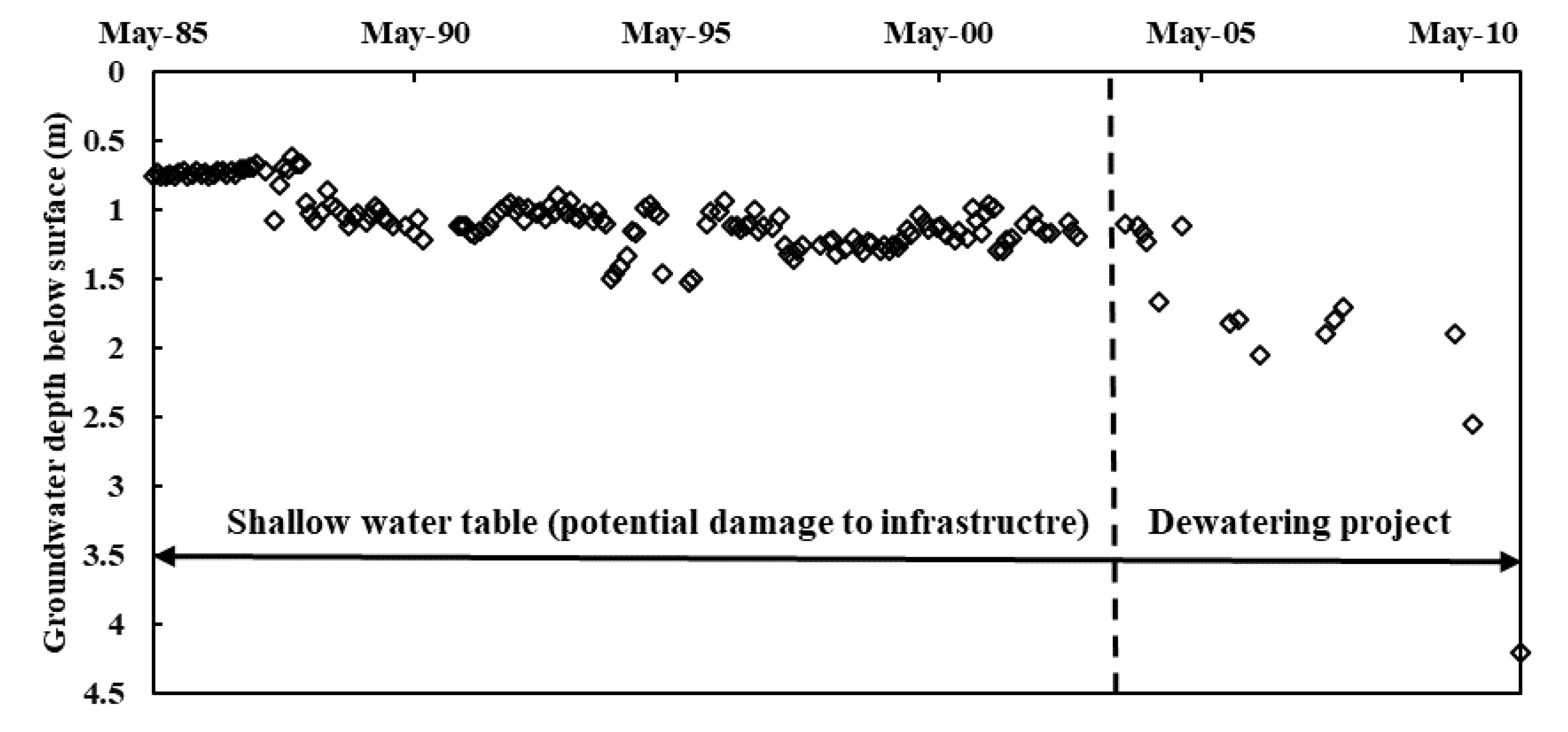
Selected groundwater monitoring wells lie in Kuwait City and are shown in Figure 1. Table 1 summarizes the key features of these wells. The groundwater table in the study area is generally shallow. The depth of groundwater table ranges between 1.0 m near the coastal line, to more than 15.0 m in the landward direction. Generally, the water table follows the ground surface topography, which gently slopes from the land towards the coast. The Ministry of Electricity and Water (MEW) has monitored the groundwater water fluctuations on a monthly time scale since 1985. The primary concern of city officials is the development of shallow water table, which may cause damage to urban infrastructure. The water table becomes very shallow in areas that are very close to the coastal line where the topography is flat and is only few meters above mean sea level. Figure 2 demonstrates groundwater level fluctuation at DE-1A well, which is located within 1 km from the coast. Historical groundwater levels there vary between 0.5 and 1.5 m below the ground surface. The shallow water table makes buried infrastructure utilities and building basement highly vulnerable to flooding. The MEW operates dewatering projects to increase groundwater depth in order to preserve buried infrastructure utilities as well as buildings basements from damage.
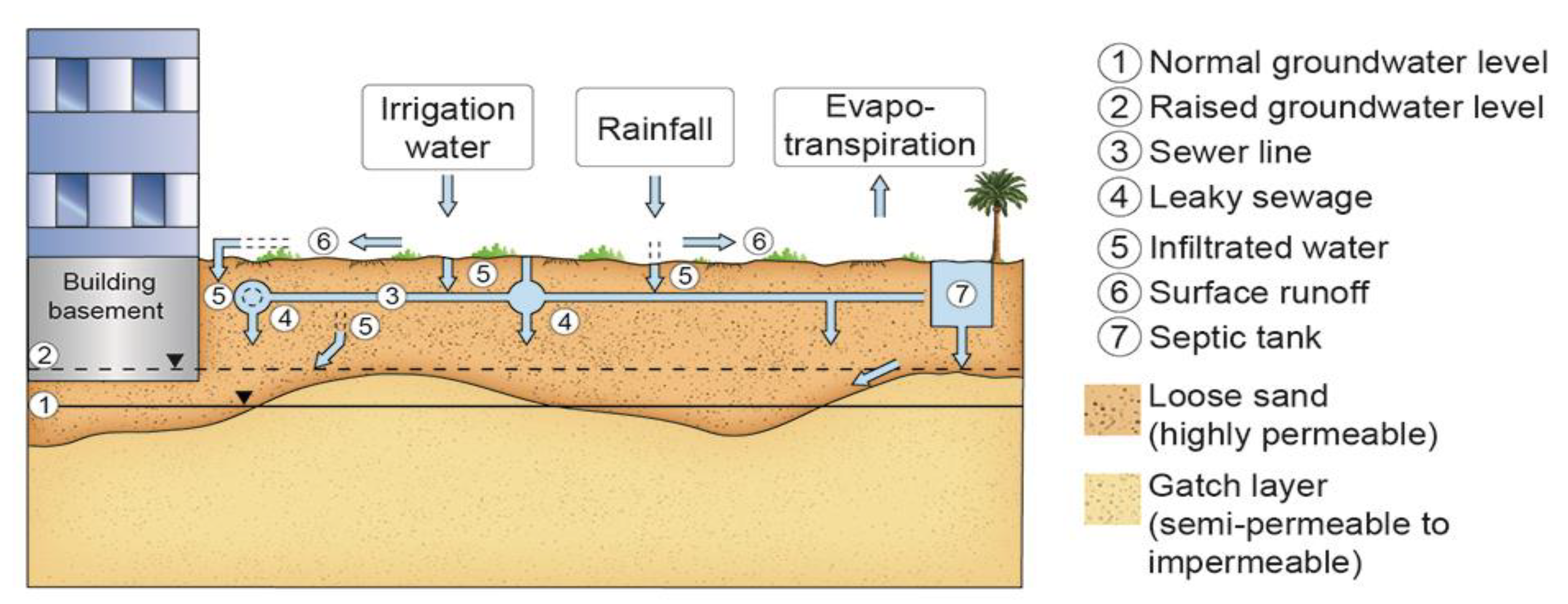
It is essential to establish a hydro-stratigraphic framework for the study area in order to select an appropriate modeling scheme, thus Figure 3 shows a conceptual hydro-stratigraphic model for the study area. In terms of soil lithology, the shallow subsurface (to a depth of 20 m) of Kuwait City is generally composed of a highly hydraulically conductive granular silty sand with patches of cemented discontinuities. The granular deposits are underlined by a low conductivity layer of gatch soil. The underlying gatch layer contributed to the occurrence of a perched water table within sandy deposits.
The intensive urban development in Kuwait City has substantially reduced the natural recharge to the perched aquifer due to urban storm water drainage systems and increased catchment imperviousness. Previous research on the study area has estimated that only 13.8%–14.6% of the total recharge to the perched water table is from natural sources (including lateral inflow and upward leakage from deeper groundwater) while the remainder comes from man-made activities [15,20]. On the other hand, the urban development has also decreased evaporation from the shallow water table.
Previous efforts in modeling groundwater level fluctuations at the study area have focused on either physically based numerical modeling approaches (e.g., [16,18,21]) or statistically based periodic models [22]. Due to the hydro-stratigraphic features of the study area, physically based models are limited in simulating groundwater level fluctuations due to the difficulty in estimating man-made artificial recharge activities, which are the key influencer on seasonal variation in the localized water table. In addition, the complexity and heterogeneity of the subsurface lithology of the aquifer system add further constraints to the use of physically based models where known aquifer parameters are scarce. On the other hand, periodical models did not present a robust tool for forecasting future groundwater levels as discrepancies can be found in these model’s predictions [22].
3. Methodology
Figure 4 illustrates the applied sequential modeling approach used for forecasting groundwater levels fluctuation in the study area. As mentioned in the introduction section, the temperature time series has been selected as the exogenous input for the NARX model as it is better correlated to artificial recharge activities. The following subsections explain the modeling approach shown in Figure 4 in detail.
3.1. Non-Linear Autoregressive Networks with Exogenous Input
3.1.1. Network Architecture
NARX networks are a special family of networks within ANNs. Inspired by the biological neural system, ANNs consist of nodes, which are connected by neurons in a certain manner. During the training process, weights are assigned to these neurons in order to specify the best fit, which can relate the input data and output data (targets) of the network. ANNs can be categorized based on the direction of information flow [23]. In feedforward neural networks (FNNs), nodes are arranged in layers, where input data are fed to the input layer, and pass through hidden layers to the final output layer. The flow of information in FNNs is along one direction. On the other hand, in recurrent neural networks (RNNs) information flows in the forward and backward directions. The output of RNNs is recycled as the next time step input.
NARX networks are a special type of RNNs that describe the modeled process based on a lagged input-output variable. This feature of the NARX network makes it an efficient tool for modeling nonlinear systems [24,25]. NARX networks combine ANNs with ARX (autoregressive models with exogenous input) which is a popular statistical technique for time series analysis and modeling. These combined features of NARX allow for capturing nonlinear behavior in an autoregressive time series. When the exogenous input is added to the NARX network, NARX becomes easier to calibrate as the number of parameters needed to be calibrated is reduced [14].
The common formulation for the NARX model is given by the following equation
where y(t) represents the target time series, x(t) represents exogenous time series, ny and nx are the delay of the target and the exogenous time series respectively, and f is a nonlinear function which is generally unknown (the black box function).
The black box function is regressed to the target time series by calibrating the number of hidden layers. This black box function passes the input and exogenous time series through a specific number of hidden layers, and the NARX network is trained by certain algorithms to produce the best match between the inputs and the target variable.
3.1.2. Training Algorithms
In this study, the Levenberg–Marquardt (LM) algorithm is used to train the NARX network. The LM algorithm is a widely accepted training algorithm for ANN-based groundwater time series modeling [13,26]. The LM algorithm combines the advantages of the Gaussian–Newton and steepest descent methods [27]. Essentially, the LM algorithm searches for the function minima and optimizes the solution. The LM method approximates the Hessian matrix as follows [28]:
where, w is the weight vector, is the Jacobian matrix, is the transpose matrix of , is a learning parameter, is the identity matrix and represents the vector of the network error.
Using Jacobian matrix with identity matrix term ensures that the Hessian matrix is always positive. This significantly reduces the computational cost of the algorithm. Hence, the LM method is considered more efficient as a training algorithm in comparison to other second order methods [29].
3.2. Data Preprocessing
The first computational step in the presented modeling approach is detrending the groundwater level data. Due to the increase in manmade recharge activities, the examined raw groundwater wells data show an increasing trend in the water table (i.e., the water level becomes shallower). The detrending procedure is meant to eliminate the effect of any external influence on the data. Dewatering projects or artificial recharge activities are difficult to estimate; hence, the detrending procedure will effectively improve the NARX model procedure. Another key advantage achieved when detrending raw groundwater data is that it ensures specifying the significant number of autocorrelation lags for the groundwater time series as highly trended time series will likely have strong autocorrelation coefficients [30,31].
One of the widely accepted detrending procedures in groundwater modeling is the first order polynomial detrending procedure (linear detrending) [32,33]. A linear regression model is fitted to the groundwater data based on a least squares criterion. The detrended groundwater signal (remainder signal) is then used as an input for the NARX model, simulating groundwater fluctuation independently of the effects of external fluxes. The fitted trend is then added back to the simulated groundwater levels by NARX to include the effect of the external fluxes.
3.3. Autocorrelation and Cross-Correlation Analysis
The basic premise behind autoregressive models is the assumption of the existence of a significant autocorrelation within the time series. The autocorrelation can be used to construct an autoregressive model, which predicts future values based on the current values of a time series. In order to test for autocorrelation within a time series, the correlogram test is used. The objective is to analyze the detrended monthly groundwater time series to determine the degree of correlation between adjacent values. The temporal separation interval is called lag and is denoted by the letter tau τ. Initially, each series of detrended monthly groundwater level data was standardized by the following equation:
where is the detrended monthly groundwater level in month , is the time series mean and is the time series standard deviation. The standardized series has a zero mean and a unity standard deviation. The correlogram r was then obtained for the series at lag as follows:
where is the mean of the sample of values of the standardized series . The value of Equation (2) is bounded between −1 and +1. In the correlogram, the upper and lower lines define the confidence bounds (C.B.). Confidence lines are usually indicated for a significance level .
where represents the quantile function of the standard normal distribution. If the correlogram computed according to Equation (2) exceeds the upper (or lower) confidence line, then a significant positive (or negative) autocorrelation exists within the time series. If the correlogram does not exceed either the upper or the lower confidence lines, then the null hypothesis of no significant autocorrelation is indicated.
To confirm the appropriateness of the selection of the temperature time series as the exogenous input to the NARX model, a cross-correlation analysis is performed. The Pearson correlation measures the linear dependency between two time series. In this study, the Pearson correlation is used to assess the strength of the association between the detrended groundwater level data and the selected exogenous input for the NARX model.
3.4. Model Validation and Performance Assessment
The developed model was validated based on the conventional practice of chronologically dividing the observed data into training and validation subsets. However, in order to ensure the robustness of the model performance, a rolling validation procedure with modification was adopted [34]. In this procedure, the NARX model is constructed using 60% of the available data with 80% of the subset used for network training and 20% used for network validation. Next, the network is constructed using 80% of data with the same data portioning percentages for training and validation purposes. Lastly, 100% of the data is used to construct the NARX model at the third-round validation procedure. This rolling validation procedure can effectively ensure that the NARX model is not overfitted.
At each of the three validation rounds, three performance metrics are calculated to assess NARX performance, namely, the coefficient of determination (R2), the mean absolute error (MAE), and the Nash–Sutcliffe coefficient (NASH). The coefficient of determination indicates the strength of association between the observed and simulated targets, and ranges between zero and one, where zero indicates no statistical association, and one indicates a perfect match between the observed and simulated targets. R2 is defined as the square of the well-known Pearson correlation coefficient. In this case, R2 does not directly measure how good the predictions are (unlike how Pearson correlation does), but rather it assesses the quality of a predictor that might be constructed from the model. The following equation calculates R2 for the simulated and observed groundwater depths values:
where represents the observed groundwater depth at time step i, represents the simulated groundwater depth at time step i, represents the mean of the observed groundwater depth time series, represents the mean of the simulated groundwater depth time series and represents the number of time steps in the validation period.
The second criterion used here is the MAE, which quantifies the variation of simulated targets from observations in an objective manner according to the following equation:
The third criterion used is the Nash–Sutcliffe coefficient, which is a well-established performance metric for hydrological models [35]. The NASH ranges between -− and 1 where below zero values indicting that the observed time series mean is a better predictor than the simulated values [36]. The following equation is used to calculate NASH:
where represents the number of time steps in the observations time series.
According to Equation (8), the NASH assesses the performance of the model within the validation period relative to the complete observation dataset variation from the mean. The advantage of using the NASH for the proposed model assessment is that it assures that the variability of the modeled system is adequately represented whenever the NASH values are greater than zero.
4. Results and Discussion
4.1. Modeling Results
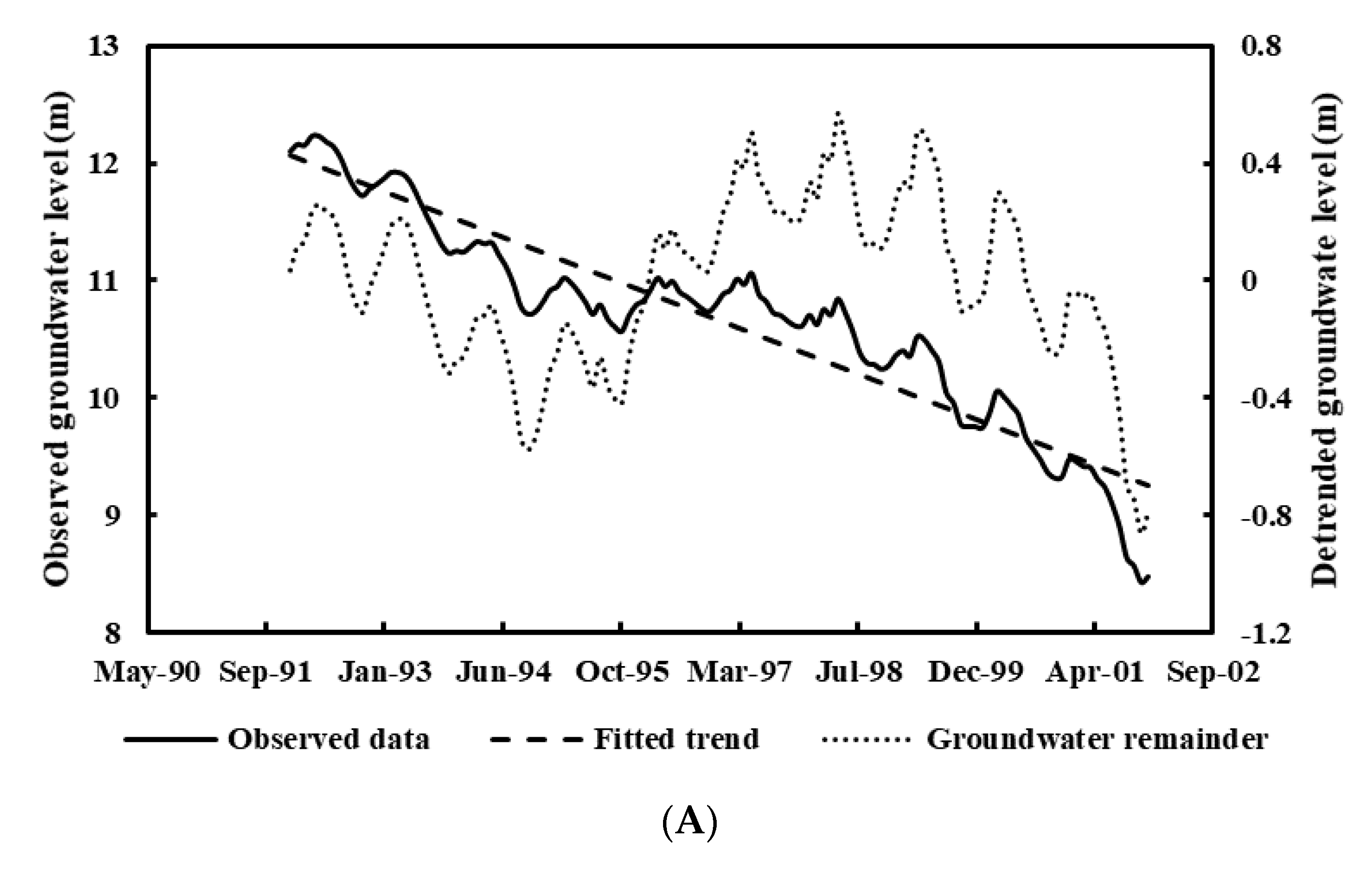
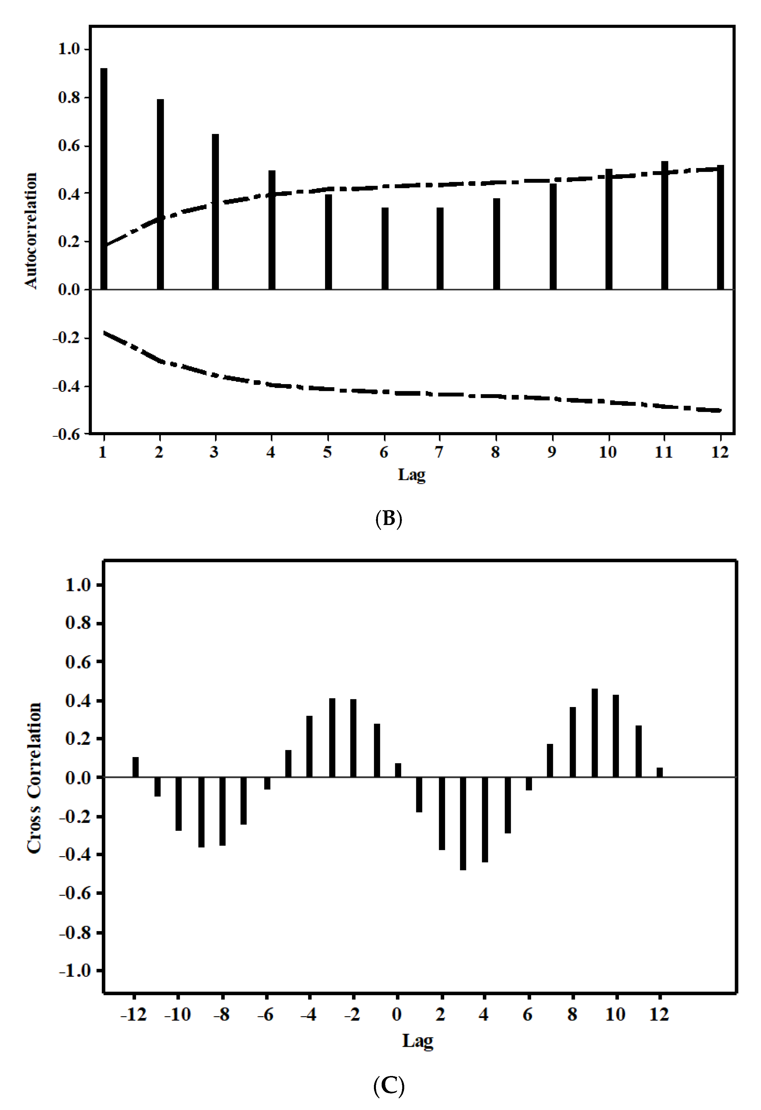
The modeling approach, which is illustrated in Figure 4 and described in detail in the previous section, was implemented to the four selected wells in the study area. Well BN-1A was used as an illustrative example for the obtained results. Figure 5A demonstrates the detrending procedure results for well BN-1A. Apparently, the raw groundwater depth data has an obvious decreasing trend (i.e., water table becomes shallower) due to the increase in man-made recharge activities over time. The detrended groundwater dataset (remainder) was then used for the next step of the modeling approach, which is the autocorrelation and cross-correlation analyses. Figure 5B shows the autocorrelation function applied to the remainder groundwater signal for well BN-1A. The upper and lower bounds drawn in the figure designate the correlation significance limit. Detrending raw groundwater data before applying the autocorrelation test assures that the specified lag time is not influenced by the long-term trend caused by the increase of recharge activities over time.
It was found that the detrended groundwater signal for well BN-1A exhibits a strong and significant positive autocorrelation for up to four lags. Accordingly, the target delay time term in Equation (1) was set equal to four. The target delay term will account for the autocorrelation in the groundwater data. On the other hand, the cross-correlation analysis between the detrended groundwater depth data and temperature time series demonstrates that a significant and negative third lagged correlation equal to −0.48 exists between the groundwater depth and average monthly temperature (Figure 5C). Accordingly, the exogenous input delay time term is set equal to three. The highly correlated temperature-groundwater depth time series emphasizes the proposed hypothesis, that the rate of artificial recharge activities can be reflected in the NARX model using the temperature dataset. Table 2 summarizes the autocorrelation and cross-correlation analysis results and the associated selection of target and exogenous delays for the four examined wells in the study area. Similarly, for the other three wells, the target input delays and exogenous input delays were set based on the computed correlations shown in Table 2.
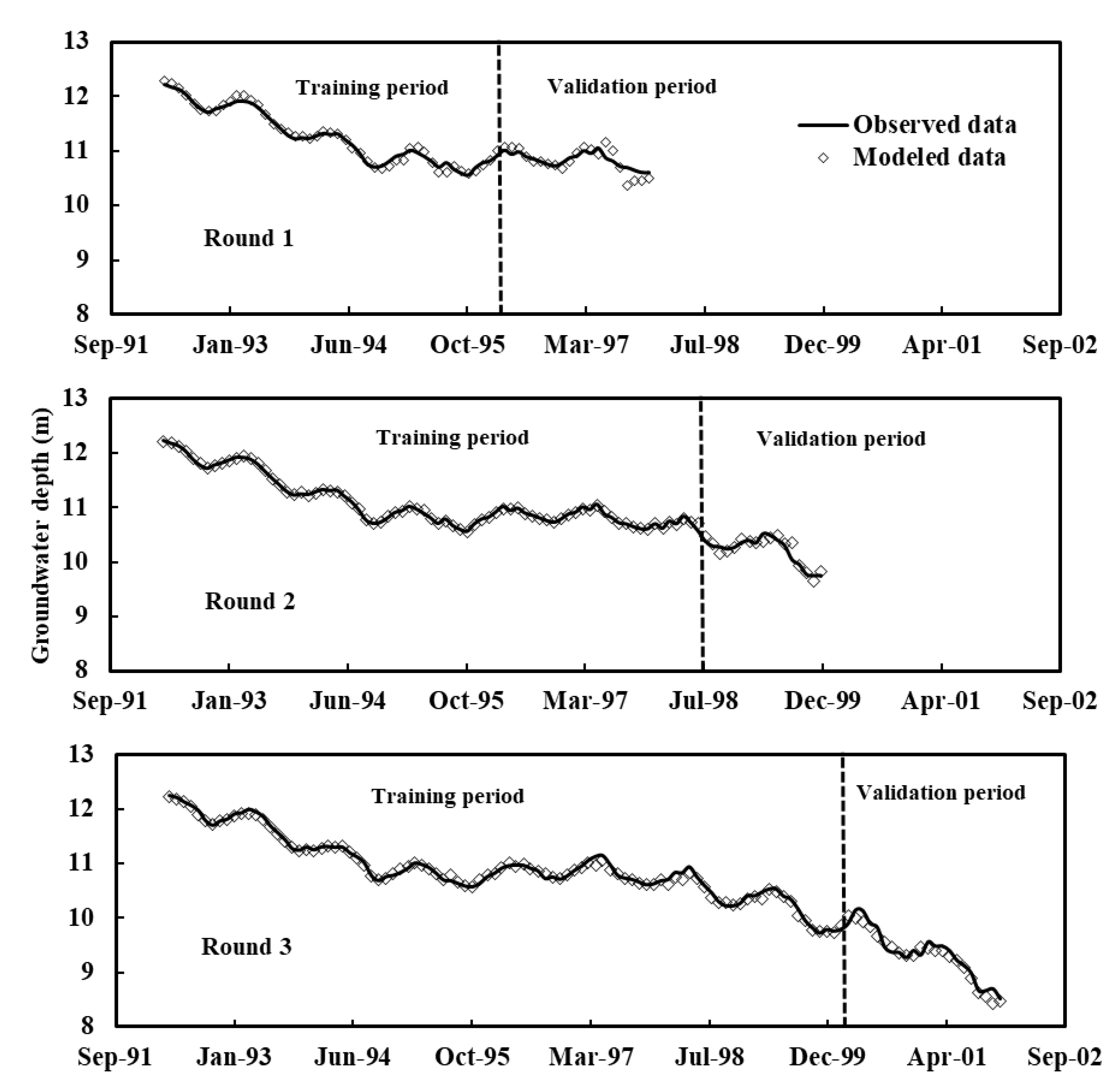
The best performing NARX models were obtained by calibrating the number of hidden neurons for each well. Table 3 shows the calibrated hidden neurons for each well corresponding to the best performing NARX network. The computed model assessment metrics can also be found in Table 3. It is important to consider all performance metrics to assess model adequacy in order to avoid contradictory results. In the current study, the performance metrics for each study site at each calibration round show that the model can efficiently predict groundwater variability. This finding is supported by the values of the NASHs and coefficients of determination computed at each validation round. It is worth mentioning here that there is an increasing trend of the NASH and the coefficient of determination as the number of data points used to build the model increases. This is considered reasonable as shorter datasets which were used in validation round 1 (only 60% of the data) or in round 2 (only 80% of the data) may not adequately represent the long-term groundwater level behavior. Hence, it is recommended to use sufficient and continuous groundwater level data for constructing the NARX model. The data period considered in the current study for the monthly groundwater level data (Table 1) are comparable with previous artificial intelligence modeling studies, which used comparable time spans for monthly groundwater data modeling (e.g., 9 years period [37], 10 years period [38], 11 years period [39], and 9 years period [40]).
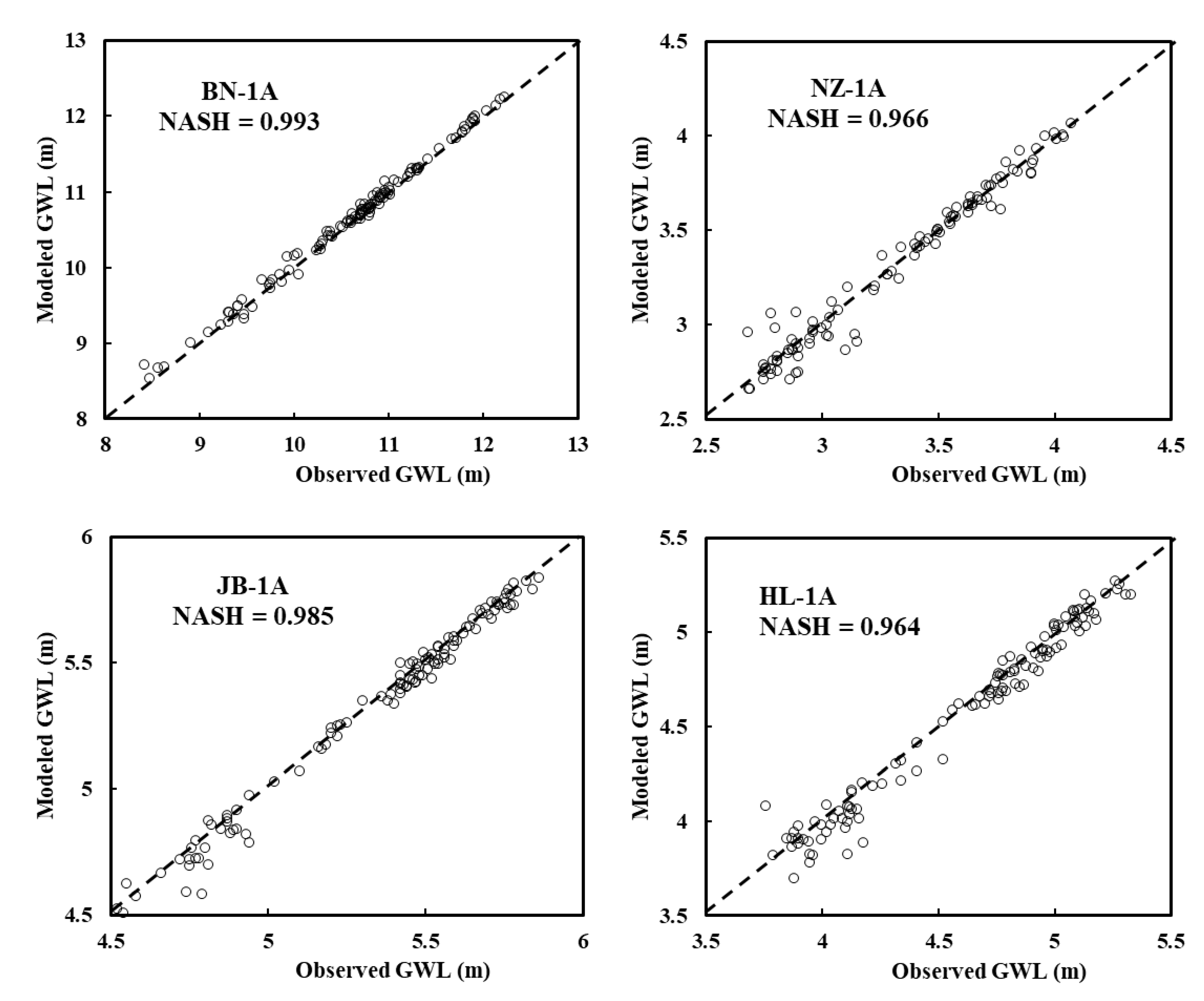
Figure 6 shows the observed and modeled groundwater levels at the BN-1A well at all validation rounds. It is evident that the model can capture the long-term trends as well as the seasonal variability of the observed data. It is shown that the duration of the training period is significantly influencing the quality of the matching between observed and modeled data. Longer training period will eventually result in better model performance. This result is reasonable as longer training data implicitly guarantee further information regarding the hydrological behavior of the modeled system. Figure 7 shows the modeled levels versus the observed groundwater levels for all examined wells with respect to the perfect 1:1 line fit. It is evident that there is no observed bias in the modeled results. A random scattering of points above and below the perfect match line implies that the model neither overestimates nor underestimates the target data. In addition, it is worth noting that the NARX models are better performing in wells where groundwater level is deeper. As described in study area section, the groundwater table follows land topography, which slopes gently from land toward the coast. Consequently, better performance of the NARX models is observed as land surface above mean sea level (m.s.l.) becomes higher. Namely, the NASH is equal to 0.993 at BN-1A well where groundwater depth is within 8.42–12.23 m and ground surface elevation is at 27.74 m above m.s.l. in comparison to the NZ-1A well, where NASH = 0.966, groundwater depth is within 2.68–4.07 m range, and ground surface elevation is at 16.45 m above m.s.l. This can be interpreted as deeper groundwater is less affected by the artificial recharge activities. The pathway for deeper water table will make the percolating water highly vulnerable to evaporation and transpiration, and thus, the effect of artificial recharge in raising the water table will be reduced.
The results shown in Figure 6 and Figure 7 indicate that the NARX modeling technique developed in the current study is a reliable approach for the modeling groundwater level fluctuation in urbanized and arid aquifers. Including monthly temperature data to overcome the difficulty of measuring artificial recharge inputs to the groundwater systems was found to be effective. NARX network models have been shown to be effective in modeling groundwater levels in the study area even without using precipitation as an exogenous input for the network. Therefore, the presented modeling approach provides a novel forecasting tool for water managers in the study area for short-term assessment of shallow water table dynamics. The presented methodology could be used at other study areas with similar hydro-lithological settings. However, the presented approach cannot be generalized for other study areas where natural recharge through precipitation is a significant contributor in raising the shallow water table.
4.2. Comparisons with Previous Studies
The results of the NARX modeling approach obtained in this study generally agree with the previously conducted research in this field (e.g., [11,12,13,14,41,42,43,44]). In particular, the results confirm the suitability of NARX in efficiently modeling groundwater level fluctuations. In terms of the performance of statistical metrics, the R2 values obtained from the current study for all examined wells ranged between 0.762 to 0.994 which are comparable to similar studies which used similar neural network approach (e.g., Guzman et al. [14] obtained R2 values ranging between 0.83 and 0.92 when using ANNs for modeling daily groundwater levels fluctuation). In addition, the performance of statistical metrics for the current study indicate that the developed modeling approach efficiency is even comparable with other data driven approaches such as support vector machine (SVM), which usually gives more accurate results [45].
However, none of the previous research has examined the suitability of NARX in modeling groundwater level dynamics in an urbanized aquifer system under arid climatic conditions. In this studyf, this gap has been bridged and the results for NARX applications in such aquifer systems are promising. Temperature time series have been used as exogenous inputs for the NARX networks in order to reflect the artificial recharge rate with time. Rajaee et al. [46] reviewed 67 recent studies published between 2001 and 2018 that used artificial intelligence methods to forecast groundwater levels, none of which solely used temperature for groundwater levels predictions. The appropriateness of using the temperature time series is strictly tied to the unique hydro-stratigraphy, shown in Figure 3. This approach has been shown to be effective in reflecting the intensity of artificial recharge, and thus, it can be considered a valuable tool for urban water managers in regard to supporting groundwater table control decisions.
The utility of the NARX approach in modeling groundwater levels in the study area was found to be superior to other statistical or physically based modeling approaches applied to the same study area. The MAE obtained for the examined groundwater wells in the current study is approximately 50% less than the MAE obtained using periodic statistical models [22]. Unlike the periodic statistical models, the NARX approach was found to be capable of representing groundwater level variability with no discrepancies between the observed and modeled groundwater values. By comparing the results of the current study with numerical simulations results, which were conducted at the study area (e.g., [16,20,21]), it was found that the NARX model can predict groundwater level fluctuations without the need for detailed aquifer parameter measurements. These measurements are often unavailable or only describe aquifer heterogeneity to a limited degree. On the other hand, the presented approach only requires groundwater and temperature data, which are widely available. Thus, the proposed methodology can be easily applied to similar aquifer systems.
5. Summary and Conclusions
This study has explored the suitability of NARX network models in modeling groundwater level fluctuations in urbanized and arid aquifers systems. The selected study area was in Kuwait City, the capital of the State of Kuwait. A modeling approach was presented and implemented for four selected groundwater wells in the study site. Initially, the groundwater level time series were preprocessed by applying a linear detrending procedure. Autocorrelation analysis of the detrended groundwater remainder time series showed that the data exhibit strong autocorrelation coefficients. The modeling approach merely relies on temperature time series data as an exogenous input for the NARX network without the inclusion of recharge sources (e.g., precipitation).
Artificial recharge sources are the major contributor in developing shallow water tables in the study area. The basic hypothesis validated by this study is the ability of average monthly temperature to reflect these recharge intensities throughout the year. The results show that the constructed NARX networks with temperature time series as exogenous input are efficient and reliable in modeling groundwater level fluctuation dynamics.
The robustness of the developed procedure has been assessed through the implementation of a rolling validation procedure in which the methodology was applied to shorter subsets of the groundwater data. It was found that longer groundwater data inputs to the NARX network improve network performance where the R2 values are increasing significantly for three of the examined wells (NZ-1A well from 0.762 to 0.966, JB-1A well from 0.887 to 0.987, and HL-1A well from 0.765 to 0.973). Comparisons with other groundwater level fluctuation modeling techniques applied to the study site showed the superiority of the NARX-based approach (MAE was reduced by 50% in comparison with periodical models). In particular, the proposed NARX model has been found to represent the variability of groundwater levels while other periodic models have failed to do so. Unlike physically based models, the proposed NARX model is simple to use and does not require detailed site investigations.
The results of the current study generally agree with studies that are focused on using artificial intelligence methods to model groundwater level fluctuations. The topic of groundwater resources in arid regions needs to be researched further in order to provide efficient water management tools in these regions where surface water bodies are limited, and groundwater often represents the only readily available water resource. Although the methodology developed in this study was tested in selected wells in Kuwait City, it can be applied to other aquifers with comparable hydro-stratigraphic settings. Thus, it is a reliable tool for urban city planners to manage urban groundwater systems.
Funding
This research was funded under Kuwait University research sector grant: ZE01/19.
Conflicts of Interest
The author declares no conflict of interest.
References
- Bear, J.; Cheng, A.H.-D. Modeling Groundwater Flow and Contaminant Transport; Springer Science & Business Media: Berlin, Germany, 2010; Volume 23, ISBN 1402066821. [Google Scholar]
- Anderson, M.P.; Woessner, W.W.; Hunt, R.J. Applied Groundwater Modeling: Simulation of Flow and Advective Transport; Academic Press: Cambridge, MA, USA, 2015; ISBN 0080916384. [Google Scholar]
- Rajaee, T.; Boroumand, A. Forecasting of chlorophyll-a concentrations in South San Francisco Bay using five different models. Appl. Ocean Res. 2015, 53, 208–217. [Google Scholar] [CrossRef]
- McCulloch, W.S.; Pitts, W. A logical calculus of the ideas immanent in nervous activity. Bull. Math. Biophys. 1943, 5, 115–133. [Google Scholar] [CrossRef]
- Linares-Rodriguez, A.; Lara-Fanego, V.; Pozo-Vazquez, D.; Tovar-Pescador, J. One-day-ahead streamflow forecasting using artificial neural networks and a meteorological mesoscale model. J. Hydrol. Eng. 2015, 20, 5015001. [Google Scholar] [CrossRef]
- Liong, S.-Y.; Lim, W.-H.; Paudyal, G.N. River stage forecasting in Bangladesh: Neural network approach. J. Comput. Civ. Eng. 2000, 14, 1–8. [Google Scholar] [CrossRef]
- Maier, H.R.; Jain, A.; Dandy, G.C.; Sudheer, K.P. Methods used for the development of neural networks for the prediction of water resource variables in river systems: Current status and future directions. Environ. Model. Softw. 2010, 25, 891–909. [Google Scholar] [CrossRef]
- Raheli, B.; Aalami, M.T.; El-Shafie, A.; Ghorbani, M.A.; Deo, R.C. Uncertainty assessment of the multilayer perceptron (MLP) neural network model with implementation of the novel hybrid MLP-FFA method for prediction of biochemical oxygen demand and dissolved oxygen: A case study of Langat River. Environ. Earth Sci. 2017, 76, 503. [Google Scholar] [CrossRef]
- Sudheer, K.P.; Gosain, A.K.; Ramasastri, K.S. A data-driven algorithm for constructing artificial neural network rainfall-runoff models. Hydrol. Process. 2002, 16, 1325–1330. [Google Scholar] [CrossRef]
- Jha, M.K.; Sahoo, S. Efficacy of neural network and genetic algorithm techniques in simulating spatio-temporal fluctuations of groundwater. Hydrol. Process. 2015, 29, 671–691. [Google Scholar] [CrossRef]
- Izady, A.; Davary, K.; Alizadeh, A.; Nia, A.M.; Ziaei, A.N.; Hasheminia, S.M. Application of NN-ARX model to predict groundwater levels in the Neishaboor Plain, Iran. Water Resour. Manag. 2013, 27, 4773–4794. [Google Scholar] [CrossRef]
- Chang, F.-J.; Chang, L.-C.; Huang, C.-W.; Kao, I.-F. Prediction of monthly regional groundwater levels through hybrid soft-computing techniques. J. Hydrol. 2016, 541, 965–976. [Google Scholar] [CrossRef]
- Wunsch, A.; Liesch, T.; Broda, S. Forecasting groundwater levels using nonlinear autoregressive networks with exogenous input (NARX). J. Hydrol. 2018, 567, 743–758. [Google Scholar] [CrossRef]
- Guzman, S.M.; Paz, J.O.; Tagert, M.L.M. The use of NARX neural networks to forecast daily groundwater levels. Water Resour. Manag. 2017, 31, 1591–1603. [Google Scholar] [CrossRef]
- Al-Sanad, H.A.; Shaqour, F.M. Geotechnical implications of subsurface water rise in Kuwait. Eng. Geol. 1991, 31, 59–69. [Google Scholar] [CrossRef]
- Hamdan, L.; Mukhopadhyay, A. Numerical Simulation of Subsurface-Water Rise in Kuwait City a. Groundwater 1991, 29, 93–104. [Google Scholar] [CrossRef]
- Mossaad, M.; Gutler, J.; Ghoneim, H.; Senay, Y.; El-Nahhs, F. Implementation of a geotechnical monitoring program in a pilot drainage project in Kuwait. In Proceedings of the Second International Conference on Groundwater Level in Urbanized Areas, Mansoura, Egypt, 7–8 November 1999. [Google Scholar]
- Székely, F. Numerical modeling of drainage schemes in layered formations: A Kuwait City case study. Groundwater 1999, 37, 879–883. [Google Scholar] [CrossRef]
- Senay, Y. Water Level Fluctuation Analysis in the Residential Areas of Kuwait City during August 1990 - July 1991; Ministry of Electricity and Water: Kuwait City, Kuwait, 1991; Unpublished Report.
- Senay, Y.; Hamdan, L.; Yacoubi, A. Study of the Subsurface Water Rise in the Residential Areas of Kuwait, Vol 3: Hydrogeology; Kuwait Institute for Scientific Research Report No. KISR2227; Kuwait Institute for Scientific Research: Kuwait City, Kuwait, 1987. [Google Scholar]
- Sayed, S.A.S.; Saeedy, H.S.; Székely, F. Hydraulic parameters of a multilayered aquifer system in Kuwait City. J. Hydrol. 1992, 130, 49–70. [Google Scholar] [CrossRef]
- Almedeij, J.; Al-Ruwaih, F. Periodic behavior of groundwater level fluctuations in residential areas. J. Hydrol. 2006, 328, 677–684. [Google Scholar] [CrossRef]
- ASCE Task Committee on Application of Artificial Neural Networks in Hydrology. Artificial neural networks in hydrology. I: Preliminary concepts. J. Hydrol. Eng. 2000, 5, 115–123. [Google Scholar] [CrossRef]
- Abdulkadir, S.J.; Yong, S.-P. Scaled UKF–NARX hybrid model for multi-step-ahead forecasting of chaotic time series data. Soft Comput. 2015, 19, 3479–3496. [Google Scholar] [CrossRef]
- Lee, W.-K.; Tuan Resdi, T.A. Simultaneous hydrological prediction at multiple gauging stations using the NARX network for Kemaman catchment, Terengganu, Malaysia. Hydrol. Sci. J. 2016, 61, 2930–2945. [Google Scholar] [CrossRef] [Green Version]
- Khaki, M.; Yusoff, I.; Islami, N. Application of the Artificial Neural Network and Neuro-fuzzy System for Assessment of Groundwater Quality. CLEAN–Soil Air Water 2015, 43, 551–560. [Google Scholar] [CrossRef]
- Samarasinghe, S. Neural Networks for Applied Sciences and Engineering: From Fundamentals to Complex Pattern Recognition; Auerbach Publications: New York, NY, USA, 2016; ISBN 0429115784. [Google Scholar]
- Bishop, C.M. Neural Networks for Pattern Recognition; Oxford University Press: Oxford, UK, 1995; ISBN 0198538642. [Google Scholar]
- Yu, H.; Wilamowski, B.M. Levenberg-marquardt training. Ind. Electron. Handb. 2011, 5, 1. [Google Scholar]
- Aldrich, J. Correlations genuine and spurious in Pearson and Yule. Stat. Sci. 1995, 10, 364–376. [Google Scholar] [CrossRef]
- Granger, C.W.J.; Newbold, P. Spurious regressions in econometrics. J. Econom. 1974, 2, 111–120. [Google Scholar] [CrossRef] [Green Version]
- Cao, G.; Zheng, C. Signals of short-term climatic periodicities detected in the groundwater of North China Plain. Hydrol. Process. 2016, 30, 515–533. [Google Scholar] [CrossRef]
- Ghanbari, R.N.; Bravo, H.R. Coherence among climate signals, precipitation, and groundwater. Groundwater 2011, 49, 476–490. [Google Scholar] [CrossRef]
- Bergmeir, C.; Benítez, J.M. On the use of cross-validation for time series predictor evaluation. Inf. Sci. 2012, 191, 192–213. [Google Scholar] [CrossRef]
- Nash, J.E.; Sutcliffe, J. V River flow forecasting through conceptual models part I—A discussion of principles. J. Hydrol. 1970, 10, 282–290. [Google Scholar] [CrossRef]
- Krause, P.; Boyle, D.P.; Bäse, F. Comparison of different efficiency criteria for hydrological model assessment. Adv. Geosci. 2005, 5, 89–97. [Google Scholar] [CrossRef] [Green Version]
- He, Z.; Zhang, Y.; Guo, Q.; Zhao, X. Comparative study of artificial neural networks and wavelet artificial neural networks for groundwater depth data forecasting with various curve fractal dimensions. Water Resour. Manag. 2014, 28, 5297–5317. [Google Scholar] [CrossRef]
- Nourani, V.; Mousavi, S. Spatiotemporal groundwater level modeling using hybrid artificial intelligence-meshless method. J. Hydrol. 2016, 536, 10–25. [Google Scholar] [CrossRef]
- Yang, Q.; Hou, Z.; Wang, Y.; Zhao, Y.; Delgado, J. A comparative study of shallow groundwater level simulation with WA–ANN and ITS model in a coastal island of south China. Arab. J. Geosci. 2015, 8, 6583–6593. [Google Scholar] [CrossRef]
- Emamgholizadeh, S.; Moslemi, K.; Karami, G. Prediction the groundwater level of bastam plain (Iran) by artificial neural network (ANN) and adaptive neuro-fuzzy inference system (ANFIS). Water Resour. Manag. 2014, 28, 5433–5446. [Google Scholar] [CrossRef]
- Kouziokas, G.N.; Chatzigeorgiou, A.; Perakis, K. Multilayer feed forward models in groundwater level forecasting using meteorological data in public management. Water Resour. Manag. 2018, 32, 5041–5052. [Google Scholar] [CrossRef]
- Asefa, T.; Wanakule, N.; Adams, A. Field-Scale Application of Three Types of Neural Networks to Predict Ground-Water Levels 1. JAWRA J. Am. Water Resour. Assoc. 2007, 43, 1245–1256. [Google Scholar] [CrossRef]
- Khalil, B.; Broda, S.; Adamowski, J.; Ozga-Zielinski, B.; Donohoe, A. Short-term forecasting of groundwater levels under conditions of mine-tailings recharge using wavelet ensemble neural network models. Hydrogeol. J. 2015, 23, 121–141. [Google Scholar] [CrossRef]
- Jeong, J.; Park, E. Comparative applications of data-driven models representing water table fluctuations. J. Hydrol. 2019, 572, 261–273. [Google Scholar] [CrossRef]
- Gong, Y.; Zhang, Y.; Lan, S.; Wang, H. A comparative study of artificial neural networks, support vector machines and adaptive neuro fuzzy inference system for forecasting groundwater levels near Lake Okeechobee, Florida. Water Resour. Manag. 2016, 30, 375–391. [Google Scholar] [CrossRef]
- Rajaee, T.; Ebrahimi, H.; Nourani, V. A review of the artificial intelligence methods in groundwater level modeling. J. Hydrol. 2019, 572, 336–351. [Google Scholar] [CrossRef]
Figure 1.
Study area map showing the location of the selected observation wells.

Figure 2.
Groundwater levels fluctuation at the DE-1A well.

Figure 3.
Schematic illustration for the problem of shallow water table development in Kuwait City.

Figure 4.
The sequential procedure for the nonlinear autoregressive modeling approach with exogenous input, (NARX)-based approach, for modeling groundwater level fluctuation in urban aquifers.
Figure 4.
The sequential procedure for the nonlinear autoregressive modeling approach with exogenous input, (NARX)-based approach, for modeling groundwater level fluctuation in urban aquifers.

Figure 5.
(A) Groundwater levels detrending procedure for well BN-1A. (B) Autocorrelation function (correlogram) applied for groundwater levels remainder at well BN-1A. Upper and lower dashed lines designate significant correlation limits. (C) Cross correlation between groundwater depth remainder and monthly average temperature at well BN-1A.


Figure 6.
Observed and modeled groundwater levels for well BN-1A at different validation rounds.

Figure 7.
Modeled versus observed groundwater levels for all examined wells with respect to the perfect 1:1 match line.
Figure 7.
Modeled versus observed groundwater levels for all examined wells with respect to the perfect 1:1 match line.


Table 1.
Selected observation wells in the study area. m.s.l.: mean sea level.
| ID | Area | Easting (m) | Northing (m) | Data Period | Ground Level Above m.s.l. (m) | Water Table Depth Range (m) |
|---|---|---|---|---|---|---|
| BN-1A | Bayan | 503,750.6 | 243,098.7 | 1992–2001 | 27.74 | 8.42–12.23 |
| NZ-1A | Nuzha | 499,402.2 | 247,349.0 | 1992–2000 | 16.45 | 2.68–4.07 |
| JB-1A | Jabriya | 502,472.2 | 244,781.0 | 1993–2002 | 23.00 | 4.52–6.08 |
| HL-1A | Hawally | 500,673.1 | 247,010.4 | 1993–2002 | 20.06 | 3.76–5.60 |
Table 2.
Auto- and cross correlations for groundwater remainder data.
| Auto Correlation for Remainder Data | Cross Correlation with Temperature | |||||||
|---|---|---|---|---|---|---|---|---|
| Well | 1st lag | 2nd lag | 3rd lag | 4th lag | 5th lag | 6th lag | Magnitude | Lag |
| BN-1A | 0.92 | 0.80 | 0.65 | 0.5 | - | - | −0.48 | 3rd lag |
| NZ-1A | 0.89 | 0.75 | 0.57 | - | - | - | −0.37 | 2nd lag |
| JB-1A | 0.93 | 0.85 | 0.75 | 0.65 | 0.56 | 0.49 | −0.33 | 3rd lag |
| HL-1A | 0.91 | 0.77 | 0.62 | 0.48 | - | - | −0.35 | 4th lag |
Table 3.
NARX models performance at each validation round (R1: round 1, R2: round 2, and R3: round 3).
Table 3.
NARX models performance at each validation round (R1: round 1, R2: round 2, and R3: round 3).
| Well | Validation Round | R2 | MAE (m) | NASH a | ID b | FD c | HL d |
|---|---|---|---|---|---|---|---|
| BN-1A | R1 | 0.971 | 0.063 | 0.964 | 1:3 | 1:4 | 30 |
| R2 | 0.992 | 0.026 | 0.992 | ||||
| R3 | 0.994 | 0.049 | 0.993 | ||||
| NZ-1A | R1 | 0.762 | 0.072 | 0.735 | 1:2 | 1:3 | 30 |
| R2 | 0.967 | 0.042 | 0.966 | ||||
| R3 | 0.966 | 0.048 | 0.966 | ||||
| JB-1A | R1 | 0.887 | 0.020 | 0.823 | 1:3 | 1:6 | 70 |
| R2 | 0.987 | 0.010 | 0.986 | ||||
| R3 | 0.987 | 0.032 | 0.985 | ||||
| HL-1A | R1 | 0.765 | 0.052 | 0.643 | 1:4 | 1:4 | 70 |
| R2 | 0.953 | 0.050 | 0.949 | ||||
| R3 | 0.973 | 0.065 | 0.964 |
a NASH = Nash-Sutcliffe coefficient; b Input delays; c Feedback delays; d Hidden layers; MAE = mean absolute error, R2 = coefficient of determination.
© 2020 by the author. Licensee MDPI, Basel, Switzerland. This article is an open access article distributed under the terms and conditions of the Creative Commons Attribution (CC BY) license (http://creativecommons.org/licenses/by/4.0/).
Share and Cite
MDPI and ACS Style
Alsumaiei, A.A. A Nonlinear Autoregressive Modeling Approach for Forecasting Groundwater Level Fluctuation in Urban Aquifers. Water 2020, 12, 820. https://doi.org/10.3390/w12030820
AMA Style
Alsumaiei AA. A Nonlinear Autoregressive Modeling Approach for Forecasting Groundwater Level Fluctuation in Urban Aquifers. Water. 2020; 12(3):820. https://doi.org/10.3390/w12030820
Chicago/Turabian StyleAlsumaiei, Abdullah A. 2020. "A Nonlinear Autoregressive Modeling Approach for Forecasting Groundwater Level Fluctuation in Urban Aquifers" Water 12, no. 3: 820. https://doi.org/10.3390/w12030820
Note that from the first issue of 2016, this journal uses article numbers instead of page numbers. See further details here.