Comparison Between Two Hydrodynamic Models in Simulating Physical Processes of a Reservoir with Complex Morphology: Maroon Reservoir


Department of Geohydraulics and Engineering Hydrology, Faculty of Civil and Environmental Engineering, University of Kassel, 34109 Kassel, Germany
*
Author to whom correspondence should be addressed.
Water 2020, 12(3), 814; https://doi.org/10.3390/w12030814
Submission received: 9 February 2020
/
Revised: 6 March 2020
/
Accepted: 9 March 2020
/
Published: 14 March 2020
(This article belongs to the Section Water Quality and Contamination)
Abstract
:Two 3D hydrodynamic models, AEM3D and MIKE3, are compared in simulating hydrodynamics of the Maroon Reservoir in southwest Iran. The reservoir has a complex bathymetry with steep walls, which makes it a good case for studying the performance of hydrodynamic models. The models were compared together and with measured water temperatures from different locations of the reservoir in a five-month period between December 2011 and April 2012. The results indicated that the AEM3D model, which uses a finite difference scheme with a purely z-level vertical discretization, showed better consistency with observations so that the AME and RMSE of the model remain below 1 °C. The MIKE3 model showed overall higher errors from 56% to 130% larger than AEM3D and the level of error strongly depends on its vertical discretization method and the turbulence model. The lowest errors by MIKE3 were seen by the k-ε turbulence model with a hybrid z-sigma discretization, while the highest errors were generated by using the sigma vertical discretization. The vertical mixing model in AEM3D model, used instead of the constant eddy viscosity or k-ε formulation, showed a better performance in modeling vertical mixing and wind mixed layer, which is another reason of observing better results by this model than MIKE3. Overall, this study shows AEM3D as a more appropriate model for simulating deep and complex reservoirs with steep slopes and walls.
1. Introduction
Dam reservoirs are man-made lakes which, although having nearly half of the characteristics of natural lakes [1], possess their own distinct characteristics in many other aspects. Physical processes in lakes and reservoirs are the main drivers of ensuing biochemical and geochemical processes occurring there and so play a key role in the evolution of their ecosystem. Hydrodynamic processes dictate stratification and mixing in lakes and reservoirs that, in turn, control the temporal and spatial distribution of nutrients and dissolved oxygen [2,3,4].
The importance of the numerous physical processes in reservoirs necessitates a deep understanding of their intricate mechanisms which, mostly, can only be achieved by advanced numerical modeling, allowing to investigate and to predict their responses to changes imposed on their environment. Hydrodynamic models are the tools to simulate the behavior of water bodies under various forcing conditions. These models are implemented with one-, two- and, nowadays increasingly, three-dimensional numerical schemes which solve spatially and temporally the differential equations describing water transport, advection and dispersion and other processes, driven by physical and climate conditions of the modeled lake.
In fact, only three-dimensional models are capable of representing the various physical processes that can take place in water bodies and aquatic environments in a realistic manner. For example, in deep and stratified lakes and reservoirs, vertical turbulent mixing can be overridden or masked by vertical density stratification [5]. On the other hand, in stratified reservoirs, there is a close relationship between vertical mixing in boundaries (boundary mixing) and inherently-3D phenomena, e.g., internal waves and internal wave braking [6], especially on sloping boundaries, where the metalimnion meets the reservoir’s benthic boundary layer [7,8], accentuated by wind forcing and bathymetry [9,10]. Both 1D and 2D models are unable to predict the mixing effects due to 3D internal wave braking and to sufficiently resolve the bottom boundary layers that would lead to large disagreements between modeled and measured variables [11]. Consequently, 3D models are needed to adequately represent the hydrodynamic processes in deep reservoirs, where the physical processes are of similar importance in all three dimensions.
Three-dimensional hydrodynamic models are typically vertically discretized using three different methods: z-level, sigma-level, or a combination of the two (hybrid). The z-level, also known as geopotential coordinates, uses Cartesian coordinates to discretize the vertical domain in which the sloping boundaries of the bathymetry are approximated by a stair-like grid. Examples of z-level models are GFDL [12], TRIM3D [13] and AEM3D [14]. The sigma-level (or sigma coordinate) discretization, firstly introduced by Phillips [15], is typically used in deep waters and applies a transformation in the vertical domain that “stretches” the domain to provide a more uniform computational domain. POM [16], SPEM [17], EFDC [18] and MIKE3 [19] are the models which employ this sigma-level vertical discretization. The latter two models are also examples of the hybrid discretization.
There is a vast domain of discussions on the pro and cons of using one or the other of the named discretization methods in hydrodynamic modeling. Various model intercomparison studies showed the difficulty of choosing the appropriate method in ocean and coastal ocean applications, as these remarkably affect the suitability of a model in a particular case [20]. For example, in ocean studies, the z-level models usually generate incorrect currents, as they are unable to represent neither barotropic nor baroclinic coastal trapped waves [21] and can cause significant errors in capturing vorticity [22]. On the other hand, the sigma models usually resolve the surface and bottom boundary layers better [20]. Sigma models work particularly well for flat or relatively-flat and mild slopes of the bottom layer. Hodges et al. [9] showed that both z- and sigma-level lake models generate different kinds of errors, originating from their numerical methods in representing boundary mixing. Particularly, where the metalimnion meets sloping boundaries, the sigma models may solve the problem of the ‘stair step’ representation of the slopes in the z-level models but insert another kind of error into the system, known as the pressure-gradient error, which leads to a distortion of the baroclinic processes. Hybrid models with z- and sigma-level discretization possess the advantage of both of the named discretization methods (e.g., [23,24,25]). Burchard and Petersen [26] showed that the combination of the two models in coastal and ocean studies results in smaller errors in baroclinic conditions compared with pure z- or sigma-coordinate models. A difficulty that occurs in using such hybrid vertical coordinates is that the transition between the two z and sigma domains can be a noticeable source of errors and discrepancies, as it can produce an excess, unnecessary boundary condition and diminish the momentum there [27].
The above are well-discussed issues in the case of ocean and coastal ocean modeling (e.g., [20]). However, for inland waters, there is only a very limited number of model intercomparison studies which mostly focus on natural lakes but exclude reservoirs. For example, Craig et al. [28] studied and developed a new vertical hybrid grid for the Environmental Fluid Dynamics Code (EFDC) model that, instead of the typical sigma-only coordinates, combines a set of sigma- and z-level coordinates. They applied this new vertical discretization approach to Lake Washington, US, for different hydrodynamic regimes and indicated that the simulated output variables of their hybrid grid model had a remarkably better agreement with the field data, especially during stratification and in the presence of sharp density gradients.
In this study, we model and assess the hydrodynamic processes of the Maroon Reservoir in southwest Iran using two 3D hydrodynamic models, AEM3D and MIKE3. Stratification, mixing and propagation of cold density currents are simulated, and their outcome is compared with water temperature observations, allowing to assess the ability of each model in capturing the hydrodynamics of this large reservoir with a complex bathymetry and steep walls. A systematic intercomparison between the two named models is carried out in terms of their power to adequately mimic measured water temperatures and so to find the most appropriate model to simulate such a complex reservoir.
2. Study Site, Data and Methods
2.1. Study Site
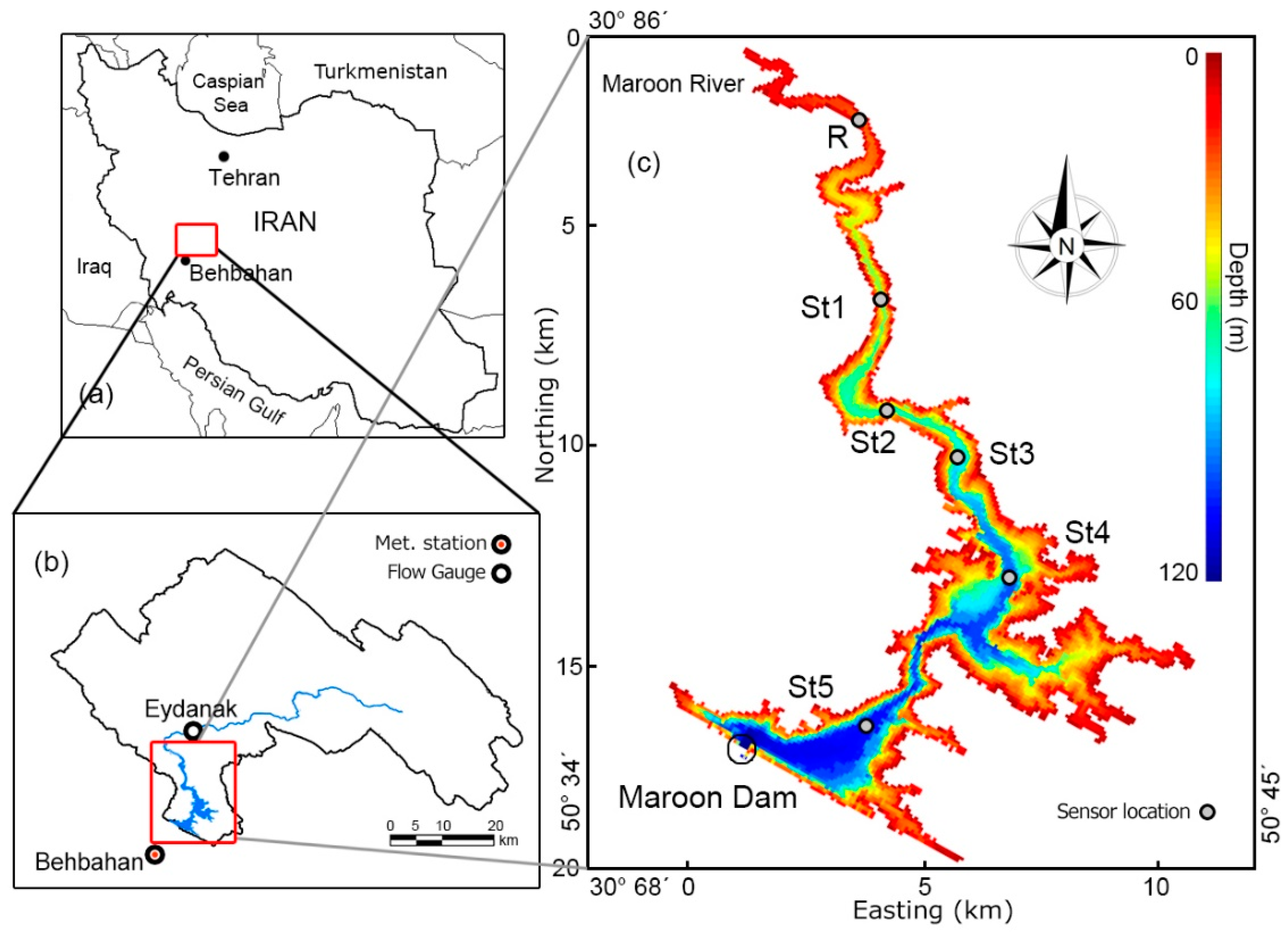
The study area is the Maroon Reservoir, a large dam reservoir located on the Maroon River in Khuzestan province in southwest Iran (see Figure 1). The Maroon dam is located in the Tang-Takab canyon, 13 km northeast of Behbahan city. The Maroon Reservoir provides downstream irrigation water needs and is also used for hydropower generation. The secondary purpose of the reservoir is to control floods of the Maroon River, one of the large rivers in Iran. The dam began its operation in 2000. Hence, it is classified as a young lake from a limnological point of view [29].
The upstream watershed of the Maroon Reservoir has an area of about 3840 km2 located in the Zagros Mountains. The main stream of the watershed, the Maroon River, is a perennial river, with a flow regime originating from rainfall and snowmelt. The long-term annual mean flow of the river, upstream of the Maroon Reservoir, is 47 m3s−1, which is seasonally highly variable. The maximum and minimum monthly flows are typically in April and October, respectively, although the flooding season starts in December.
The reservoir itself, with a surface area of 24.6 km2 and a thalweg length of 30 km (at normal pool level (NPL)), combines two basins which are connected through a deep and narrow canyon in which the flow moves downstream gravitationally. The mean depth of the reservoir, defined as the ratio of volume (1.2 × 10⁹ m3) to its surface area, is 49 m, which classifies it as a deep reservoir [5]. The mean water residence time in the reservoir is 1.27 years.
The Maroon Reservoir is classified as a warm-monomictic lake using the thermal classification of lakes suggested by Hutchinson and Löffler [30]. This implies a major stratification in summer and a major overturn and mixing period in winter. In fact, most of the Iranian lakes and reservoirs, especially, in the study region (Khuzestan province and Zagros region) are classified in this category.
The external and internal Rossby radius values [31] for the Maroon Reservoir are estimated as 289,000 and 11,000 m, respectively; i.e., they are much larger than the lateral domain size of the reservoir at up- and downstream basins (~4000–5000 m). This means that the effects of Coriolis force on the reservoir hydrodynamics can be neglected, as is done in this study.
2.2. Data
Meteorological data from the Behbahan synoptic station, 13 km southwest of the Maroon dam and the nearest meteorological station from 2011–2012 were used. The data were applied in the model uniformly over the model domain. These data include hourly records of air temperature, atmospheric pressure, wind, cloudiness and humidity and were employed as boundary conditions and partly driving force of the models. The air temperature data were corrected to the Maroon Reservoir surface elevation (at NPL) using the air temperature lapse rate of −5.5 °C km−1 suggested in [32] for the study region. As the solar (shortwave) radiation is not measured directly at the Behbahan station, it was estimated there from the measured bright sunshine data, using the FAO procedure [33], as the recommended approach for calculating solar radiation in Iran (e.g., [34,35]). Some studies (e.g., [36]) have found errors of up to 10% in the calculated peaks of hourly solar radiation using the named method in mountainous areas (in Japan). However, [35] and [37] found no significant difference between the calculated and observed solar radiation values in Iran, including the present study area (Khuzestan province).
The bathymetric data used for this study (Figure 1c) are taken from the bathymetric surveys performed by Mehrabani et al. [38]. We use daily river flow at the Eydanak gauge station (Figure 1b). These river flow data are recorded and available in an hourly scale during the flooding periods. Continuously-measured water temperature data were measured at the inflow point and five locations in the reservoir (Figure 1c) for a limited time interval. These data were measured by RBR logging sensors moored at stations R, St1, St2, St3, St4 and St5 in the hypolimnion 2 m above the bottom of the reservoir during the time of the flooding season, between December 2011 and April 2012 [38]. The recorded water temperatures at station R were used for the inflow boundary conditions and the data from St1 through St5 were used for comparisons with the models’ results.
2.3. Computational Resources
We ran the AEM3D model on the Linux cluster supercomputer of the University of Kassel with AMD 2.6 GHz processors (2 × 16 cores, 32 threads), and the MIKE3 model on a desktop PC with an Intel 3.40 GHz processor (4 cores, 8 threads) and Windows 7 operating system to simulate five months of the reservoir operation (December 2011 to April 2012). The OpenMP (Open Multi-Processing) platform was used for both of the simulations as both AEM3D and MIKE3 allow parallel computing within a multi-core (or multi-thread) node(s). The five-month simulation using OpenMP parallel computation with the grid of AEM3D (discussed later) took 7 h on the Linux cluster, while the same period by the standard (hybrid) grid of MIKE3 took ~60 h on the desktop PC. We ran the both models under hydrostatic mode which neglects the non-hydrostatic pressure effects, as using the non-hydrostatic mode requires model grids of the order of 10 m [14,19], which drastically increases simulation times. Specific details of two models’ preparations are provided in Section 2.4.2 and Section 2.5.2.
2.4. AEM3D Model
2.4.1. Model Description
The Aquatic Ecosystem Model (AEM3D) [14] is a three-dimensional hydrodynamic and ecosystem model for estuaries, lakes and reservoirs, predicting space- and time-varying water currents, temperature and salinity (in case of saline water). AEM3D uses the unsteady Reynolds-averaged Navier–Stokes (uRANS) and scalar transport equations with the Boussinesq and hydrostatic approximation. This model is a developed and improved combined version of the ELCOM [39] hydrodynamic and CAEDYM [40] ecosystem models. Albeit, in this study, only the hydrodynamic module of the model is used, as the focus is solely on the understanding of the physical processes prevalent in the Maroon Reservoir.
The hydrodynamic governing equations solved by AEM3D are listed below. The equations of the transport of momentum are the frictional shallow water equations, assuming hydrostatic pressure:
whereis the Reynolds-averaged velocity, and represent the two dimensions of the horizontal two-component space; is the free surface height, and and are the reference density and the density anomaly, respectively. is the two-component permutation tensor and is the Coriolis constant. The continuity equation is:
The free-surface evolution of is governed by vertical integration of the continuity equation (Equation (2)) for incompressible flow using the kinematic boundary conditions at the bottom (b) and the free surface (η) of the lake:
The equation of the transport of scalars (temperature and concentration (salinity)) is:
where is the scalar concentration/temperature, is the velocity obtained from the solution of Equations (1)–(3), and is the turbulent (eddy) solute/thermal diffusivity.
The numerical scheme implemented in AEM3D to solve Equations (1)–(4) is a modified adaptation of the approach used in the TRIM-3D method [13]. The latter is a semi-implicit finite difference method that numerically solves the 3D shallow-water stratified flows. The solution grid of AEM3D is a rectangular Eulerian fixed Cartesian grid (with fixed longitudinal and lateral (horizontal, Δx and Δy) grid dimensions and a vertical Δz spacing which is horizontally uniform but can vary in vertical dimension (varying vertical layer thickness). The finite difference grid stencil is based on Arakawa’s C-grid [41] in which vector values (e.g., velocity) are defined on cell faces and scalar values (e.g., temperature and concentrations) are defined on cell centers. A semi-implicit method is used for the solution of the momentum Equation (1), including an Euler–Lagrange procedure for the advection of momentum, whereas the implicit linear algebraic systems of equations arise from the discretization of Equation (3). The free-surface height for a particular time step—making up the computational burden of the AEM3D numerical method—is solved iteratively by means of an efficient iterative conjugate-gradient method. With this implicit approach, the stability of the solution is not impeded when using large time steps, as may be advocated for computational efficiency. The scalars in Equation (4) are advected using a conservative Ultimate Quickest discretization [13].
The turbulence closure in horizontal direction in AEM3D is represented by eddy viscosity. In vertical directions, there is a possibility of using two different methods: (1) a simple approach using eddy viscosity or (2) a developed mixed layer model. The latter is a development of the mixed-layer approach for vertical diffusion that is derived from the mixing energy budgets originally developed for 1D lake models [42,43,44]. Thus, the AEM3D model applies a separate 1D mixed-layer model to each water column (defined by the horizontal grid) which solves for the vertical turbulent transport. As the named mixing model does not use the eddy-diffusion differential equations, unlike the classic hydrodynamic models, there is no need for very fine vertical grid resolutions with small time steps to model vertical mixing. Further details about the equations and numerical methods of AEM3D can be found in [9,14,39].
2.4.2. AEM3D Model Preparation
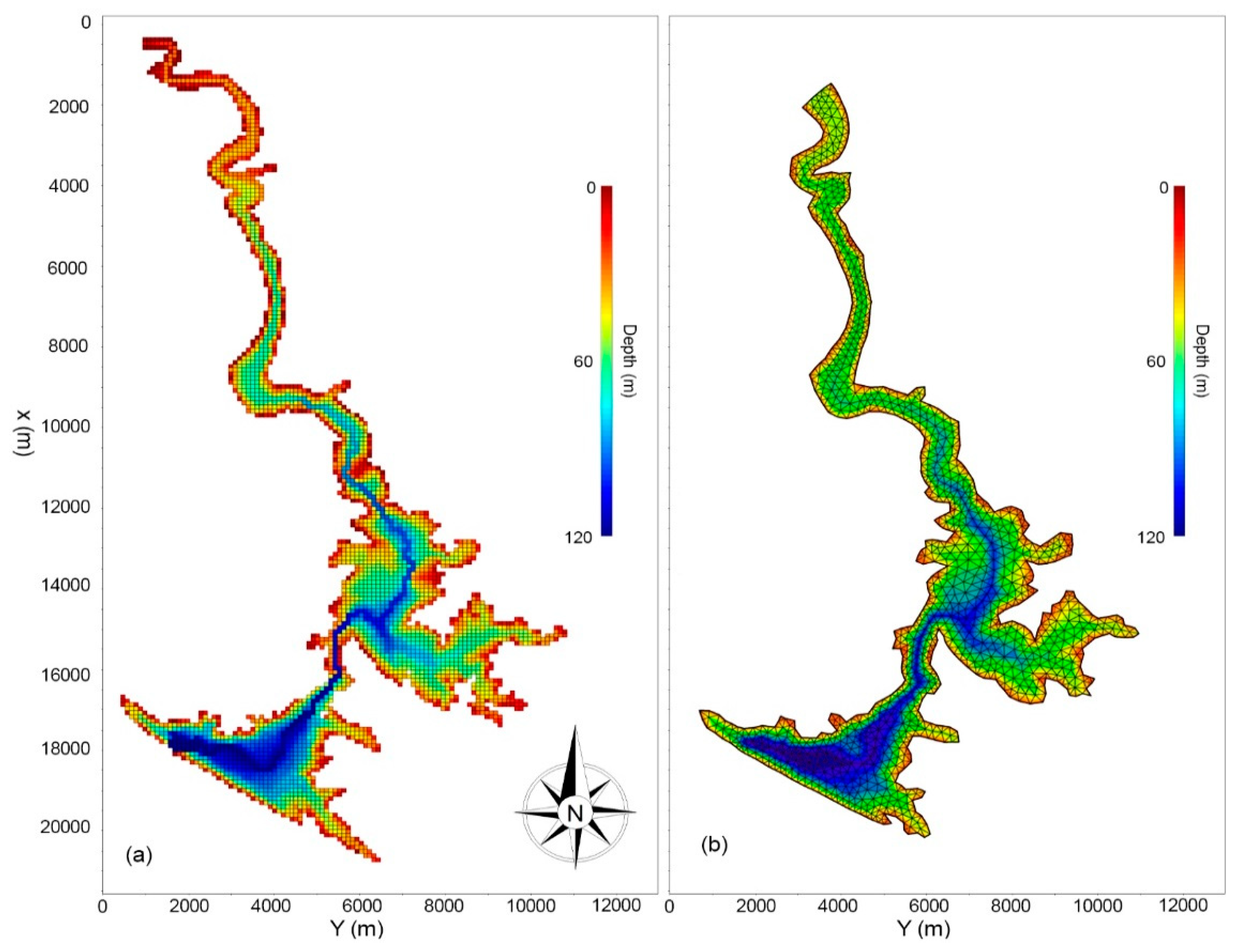
The AEM3D model grid of the Maroon Reservoir (shown in Figure 2a) uses a rectangular grid with horizontal cell sizes of Δx = Δy = 100 m and uniform layers with a vertical thickness of Δz = 1 m. This 100-m cell size was selected as a compromise between minimizing computational time and capturing the complex bathymetry of the Maroon Reservoir, including narrow and deep canyons at different sections of the water body. The entire domain of the named grid specification has 185,314 valid wet cells, of which 4803 cells belong to the free surface (at maximum water level). A time step of 40 s was chosen for the model solution advancement, considering both various (computational) restrictions and standard model stability criteria (e.g., [9,14,39]).
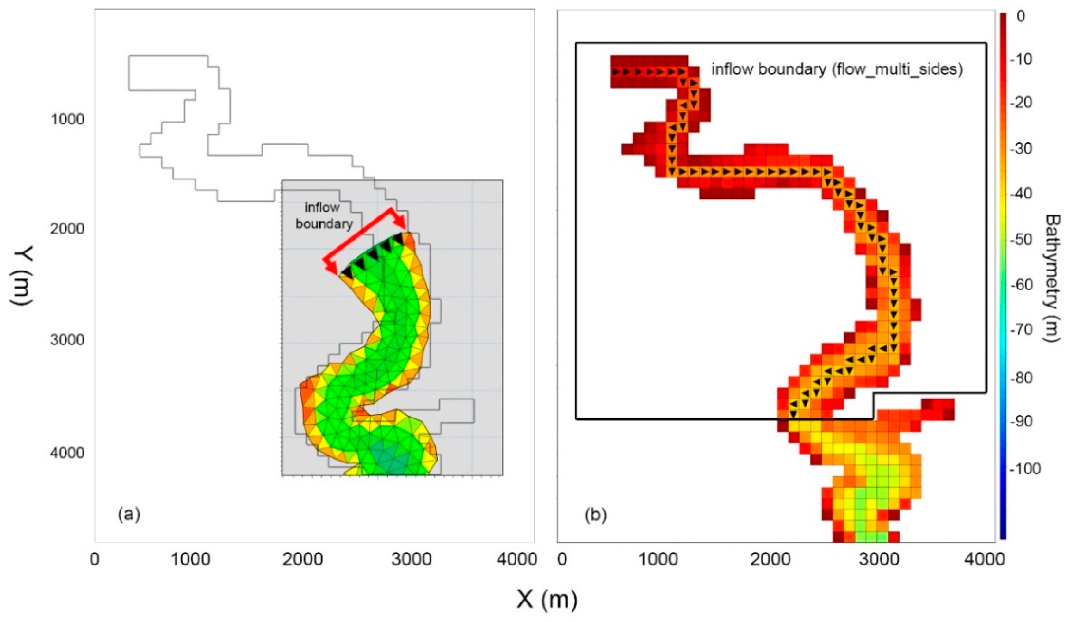
In developing the appropriate AEM3D model grid of Figure 2a, several geographical considerations of the Marron reservoir had to be taken into account. At the inflow point of the model domain, the Maroon River passes through a meandering valley into the reservoir (see Figure 1 and Figure 2a). This meandering valley is, depending on the reservoir’s water level condition, sometimes flooded and so becomes part of the reservoir’s riverine zone (high water levels), meanwhile, at other (low flow) times, it becomes only a part of the river channel’s flow path into the reservoir (low water levels). The water level in a large reservoir with hydropower facilities, like the Maroon Reservoir, can have large variations, even on a daily scale, that can lead to frequent generation of dry cells at the inflow boundaries. To tackle that issue, it is possible to use the “flow_multi_sides” feature in AEM3D which allows to define one inflow boundary as a set of multiple cells with inflow from different faces, depending on the flow direction at that location [14]. This boundary configuration lets the model simulate the river inflow into the domain in the correct direction (see Figure 3a) and provides the flow along the thalweg into the reservoir’s free surface without having any dry cells (that might cause errors). The river then flows along the thalweg with the predefined flow depth, without affecting the cells below or above it and without being enforced during that time step, and enters the reservoir, wherever the river flow meets the free surface.
2.5. MIKE3 Model
2.5.1. Model Description
The MIKE3 model [19,20], similar to AEM3D, is also based on the incompressible Reynolds-averaged Navier–Stokes equation (RANS), assuming the Boussinesq and hydrostatic conditions, i.e., vertical accelerations are neglected.
The vertical section of the model domain is discretized in MIKE3 using either sigma or a combination of the two z- and sigma-coordinates (hybrid mesh). In the latter case, the sigma coordinates are used in the upper parts of the flow domain and z-coordinates in the lower parts, close to the bottom of the domain, allowing to partly overcome the so-called “pressure gradient problem” of sigma-coordinate systems near varying bottom topography (e.g., [45,46]). The governing hydrodynamic equations have slightly different forms for these two kinds of discretization.
In z coordinates the momentum equations in x and y directions are:
where is density; u, v and w are velocities in x, y and z directions, respectively; is the atmospheric pressure, is the turbulent eddy viscosity; , , and are components of the radiation stress tensor, which transfers excess momentum due to surface gravity (wind-induced) waves to the mean flow; S is the source/sink term and and are the velocity components of discharged water from the S source/sink into the domain. The continuity equation is:
The free surface boundary condition at is:
In sigma coordinates, having applied the sigma transformation (e.g. Phillips [15]) on the governing equations, the momentum equations, Equations (5)–(7) change into:
where is the modified vertical velocity in sigma coordinates and is the velocity across a level of constant which is calculated by:
The set of the hydrodynamic equations above in MIKE3 are completed by scalar equations for temperature and solute transport, similar to Equation (4) for the AEM3D model. Further details about the governing equations of MIKE3 can be found in [19,20].
In MIKE3, the turbulence and vertical diffusivities are calculated using either a standard eddy viscosity or a k-ε formulation. The horizontal and vertical diffusivity coefficients in these formulations are empirical values which need further calibration. A careful calibration of the named coefficients was done by Rodi [47], and these values are the generally-accepted values in most modeling studies [19]. The k-ε model takes into the account the turbulent kinetic energy k (TKE) and its dissipation ε to calculate the vertical eddy viscosity. Such a k-ε formulation increases the accuracy of the model predictions in comparison to the standard eddy viscosity formulation using a constant eddy viscosity in the model [47].
In this study, the flexible mesh (FM) version of MIKE3 is employed allowing to run the simulations within reasonable computational times. In this FM version, the governing equations above are discretized over the domain by means of the finite volume method, which has become the state-of-the-art in computational fluid dynamics over the last decade. Besides being well-suited for unstructured meshes, a particular asset of the finite volume method is its high mass-conservation (flux continuity) across the different cells of the computation domain (e.g., [48]).
2.5.2. MIKE3 Model Preparation
The horizontal domain of the Maroon Reservoir was discretized in MIKE3 using the unstructured triangular mesh shown in Figure 2b. Although the grid size in the FM version of MIKE3 varies over the horizontal domain, its average size is roughly identical to that of AEM3D (100 m). The vertical mesh is discretized, as discussed, using a structured and layered mesh, which can either be entirely sigma layers, or a combination (hybrid) of z-sigma layers. In this study, we implemented both vertical discretization approaches to compare the accuracy of the two as well as with that of the z-layer discretization of the AEM3D model, allowing for vertical mixing. In that case, the same vertical layer thickness as that of AEM3D (1 m) was chosen. More specifically, in the pure sigma grid, the vertical mesh was discretized into 125 layers, which implies 1 m layers. In the z-sigma hybrid grid 50 sigma layers between the top of the domain (at 515 m) to the 50 m depth, and further 75, 1 m thick z-layers to the bottom were defined.
In the hybrid mesh, regardless of the real inflow depth, the inflow boundary condition and the flooding and drying of the model domain must remain within the sigma domain, as the free surface equation is solved in sigma coordinates. Thus, the sigma domain should not become completely dry during the simulation; otherwise, the model faces instabilities which may lead to a complete crash of the numerical computation [19]. To this avail, modifications on the inflow boundary of the reservoir, as the highest point of the reservoir’s thalweg (facing regular flooding and drying), are required. This modification (see Figure 3b) could restrict the implementation of the rigorous physics of the inflow boundary and requires changes and smoothing of the bottom topography, even in most of the basin-scale estuary models (e.g., [47,49]). In cases of lakes like the Maroon Reservoir with even steeper topography in the bottom, these modifications seem unavoidable. Moreover, since it has been shown that while sigma-coordinate models are appealing for representing smooth bottom topography well, they may induce large pressure gradient errors in the presence of steep vertical topography (e.g., [45,46]). In this study, the inflow boundary was defined by modifying the bathymetry of the riverine zone so that the depth range at inflow boundary, regardless of the real depth of the river, covered the range of the expected reservoir’s water level change. To avoid imposing unrealistic physics on the domain due to the named smoothing and changes, the distance between the inflow boundary and the location from where the real bathymetry of the reservoir begins should be taken as short as possible. To this avail, riverine zone of the reservoir was shortened by 3500 m in the MIKE 3 model domain (see Figure 3a).
2.6. Models’ Parameters
It is shown in the literature that 3D hydrodynamic models can often be used by employing the standard coefficients in the literature without being calibrated. The term “model calibration” is specifically associated with 2D models (e.g., CE-QUAL-W2) where the cross-channel horizontal direction has been averaged and the reservoir is effectively straightened. Such models have difficulties in the relationship between water surface elevation and volume because each grid cell represents a different cross-sectional area. Furthermore, 2D models have to include the relationship between the measured wind direction and thalweg direction, which varies with the wind momentum introduced into the water. For 3D models, both of these problems disappear because the shape of the reservoir has not been distorted. AEM3D and MIKE3, for instance, are volume conservative models, so that the volume in the reservoir is precisely determined by the balance of inflows, outflows and evaporation. One should note that the goal of the present work is not to estimate the water yield of the reservoir (which is highly dependent on accuracy of evaporation), but to estimate the consequences of water scalar values, i.e., temperature. These are highly dependent on the stratification, which is determined by an interaction of the entire thermal balance and the turbulence in the surface mixed layer.
The successful implementation of the 3D models without need for calibration has been clearly indicated by [11,50,51] who showed that AEM3D (formerly known as ELCOM) provided excellent agreement with field measurements for surface thermodynamics and mixing processes. Lee et al. [52] also used accepted literature values in simulating the thermal stratification and fate and transport of contaminants after a large flood event in a deep and stratified reservoir with the coupled ELCOM-CAEDYM (AEM3D) model. Their validation with field data indicated that the model performed well (within acceptable error) in simulating water temperature profiles and vertical mixing in both normal conditions and during the flood event. Consequently, following the named studies, we used the models in this study also by accepting the literature values. The parameters and their values used in AEM3D and MIKE3 are shown in Table 1 and Table 2, respectively.
2.7. Methodology and Models’ Evaluation
The simulated water temperature values at the sensor locations and sensor heights (2 m above bed) were extracted from the models’ results and were compared to the measured values by the sensors. Then the simulations were compared together to perform the model intercomparison.
Model performance and accuracy was evaluated using the absolute mean error (AME) and the root-mean-square error (RMSE):
where is the observed value measured at the station, is the corresponding value simulated by the model and is the number of data values. The named values were calculated for the water temperature. Correlations between simulated and observed temperatures were calculated after removing trends from the time series.
3. Results and Discussion
3.1. General Results of Hydrodynamics
In this subsection, the hydrodynamics obtained with the AEM3D and three variants of the MIKE3 model are illustrated and compared to each other over the five-month simulation horizon. For MIKE3, we mainly use its k-ε turbulence model and hybrid discretization, as this combination turns out to provide the most precise results. However, other variants of the MIKE3 model (i.e., sigma and z-sigma vertical discretizations and eddy viscosity turbulence model) are also evaluated (see Table 3 and Table 4). A brief statistical evaluation of the models (discussed below) at the different stage stations is also illustrated in Figure 4.
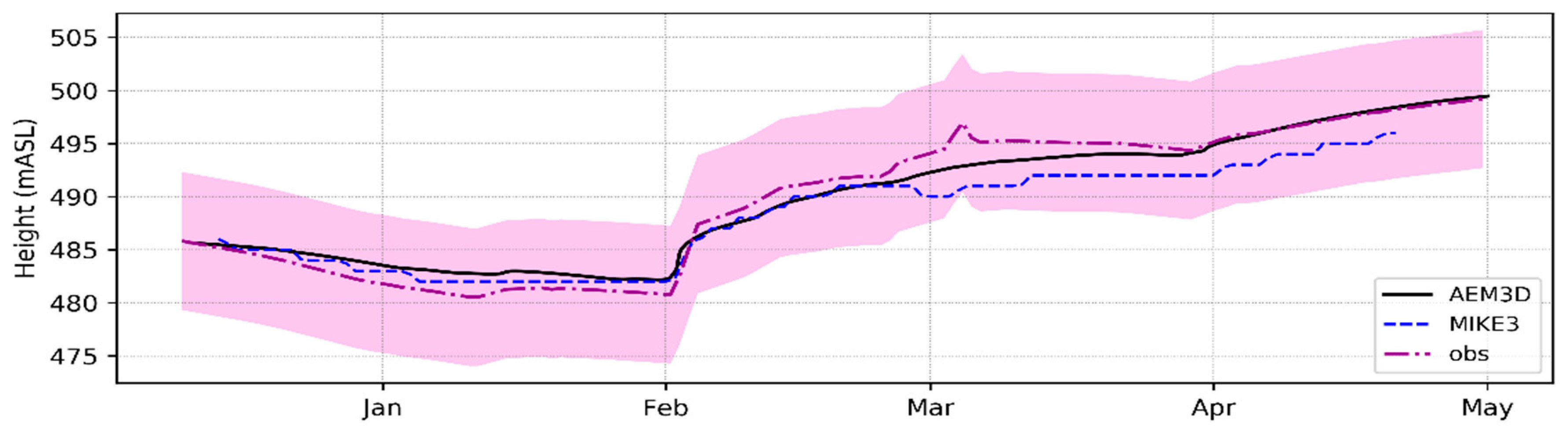
Figure 5 and Figure 6 show transient hydrographs of the simulated and observed water levels and the simulated and observed temperatures at the five gauging stations, respectively, obtained with the two models. As can be seen from the two figures, both models predict the water balance and the water level reasonably well. The slight discrepancies (not statistically significant) between the modeled and observed water heights arise from the step-like introduction into the model of the steep walls of the Maroon Reservoir. This results in slightly different volume–height relationships in the model, as the given model discretization cannot completely resolve the complex morphology of the reservoir in these points. A potential solution to overcome this bias would be to refine the model grid. However, Hodges et al. [53] showed that doing so in a hydrostatic model, although this might lead to slightly better results, will change the balance between numerical dissipation and numerical dispersion of the internal waves front. This would result in waves with greater artificial steepening which, however, does not imply a better representation of the real physics of the problem. Furthermore, for practical purposes, refining the grid entails long and, in case of limited computational resources, prohibitive simulation times.
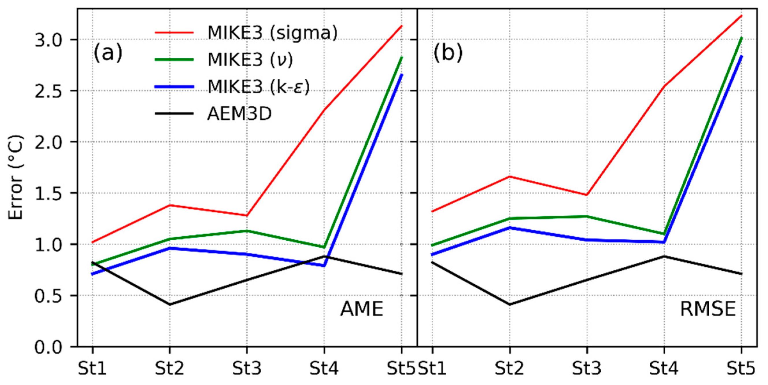
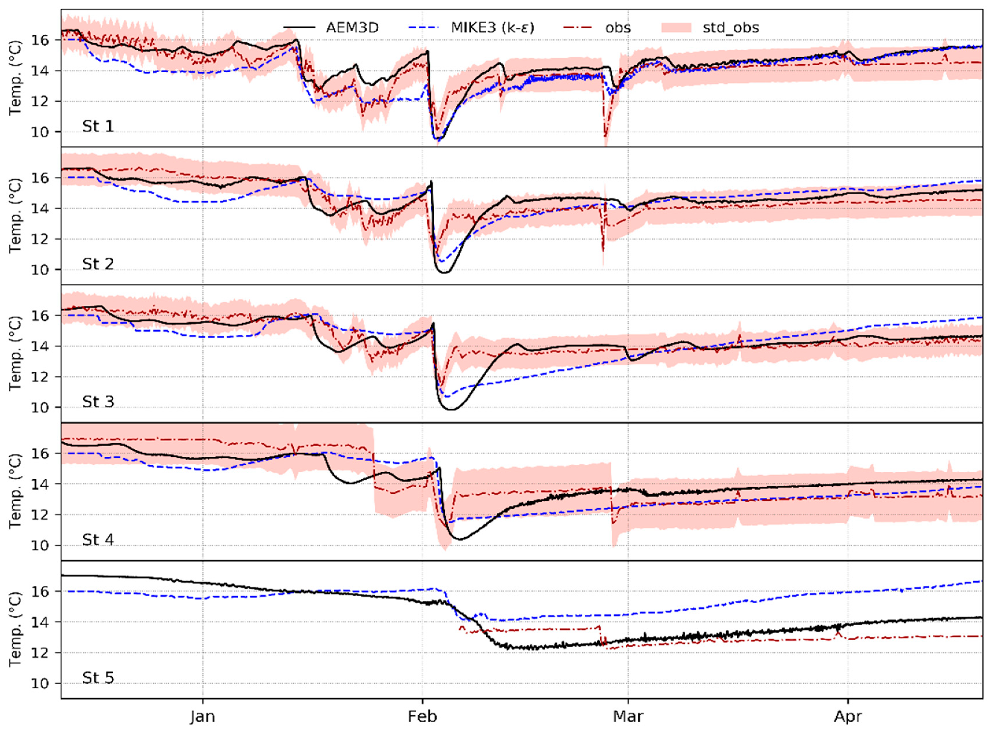
The statistical values listed in Table 3 indicate that the AEM3D model’s simulations are very well consistent with the measured data. Both the AME and RMSE at the five measurement stations are all well below 1 °C (also seen in Figure 4), and their average for all stations is only ~1 °C, which is more remarkable, given that the total temperature range over the whole simulation period (December–April) is 10–29 °C. Moreover, these error measures are lower than those obtained in similar AEM3D model applications (e.g., [50,54,55]). Continuous plots of the observed and simulated temperatures are illustrated in Figure 6 and show that the AEM3D-modelled temperatures fall within the range of the standard deviation of the observed data.
This implies that the model predictions remain within the uncertainty range of the observations and indicates that the AEM3D model provides good consistency with field measurements by using the accepted values in the literature without separate calibration. Consequently, we believe that the AEM3D model is well capable in capturing water temperature, as the key parameter of the density variations and the hydrodynamic model, in the Maroon Reservoir.
As mentioned in the theory section, MIKE3 has two turbulence models implemented: the k-ε model and the constant-eddy-viscosity model. In addition, the vertical model discretization in this model can be done in Cartesian z-sigma hybrid or pure sigma coordinates. Figure 7 shows the MIKE3-simulated water temperatures using these two vertical mixing models in combination with the two named discretization variants. Table 3 and Table 4 list the quantitative statistics obtained at the five gauging stations obtained with these MIKE3-variants, as well as those of the AEM3D model.
All Figure 7 and Table 3 and Table 4 indicate that the k-ε variant of MIKE3 has smaller errors than the constant-eddy-viscosity model variant, a finding which is consistent with that of previous studies (e.g., [47,56]). In fact, the RMSE of the temperatures of the latter turbulence model is 9% larger than that of the former k-ε model (see Table 3). This is also visually corroborated by the simulated temperature curves in Figure 7, which run closer to the observed ones for the k-ε than for the constant-eddy-viscosity model.
Regarding the effects of the vertical model discretization in MIKE3, using the (superior) k-ε turbulence model, Table 1 shows that the results using the sigma discretization are much worse than those of the hybrid z-sigma discretization, as the RMSE values of the sigma discretization variant are roughly 35%–46% larger than those of the hybrid variant. This result confirms the studies by [57] and [45] who found that the sigma discretization in steep topographies results in significantly higher errors due to under-/overestimating of the baroclinic pressure terms and sharp density gradients.
This overestimation of the water temperature by the sigma discretization is also seen in Figure 7, and it is more pronounced in the downstream locations after the February 2 flood, where up to 2 times higher simulated than observed temperatures are obtained by this MIKE3 discretization variant.
Table 3 indicates that all three model variants of MIKE3 give results that are consistent with the observations. This is also supported by the acceptable correlation values between simulated and observed data, listed in Table 4, although MIKE3 slightly overestimates the water temperature.
Both Figure 7 and Table 3 indicate that the MIKE3 k-ε model variant has smaller errors than the constant-eddy-viscosity model variant, a finding which is consistent with that of previous studies (e.g., [47,56]). In fact, the RMSE of the temperatures of the latter turbulence model is 9% larger than that of the former k-ε model (see Table 3). This is also visually corroborated by the simulated temperature curves in Figure 7, which run closer to the observed ones for the k-ε model than for the constant-eddy-viscosity model.
More detailed inspection of Figure 7 and Table 3 and Table 4 shows that the RMSE of the different station locations vary. Higher error values are generally seen at downstream stations (e.g., St4 and St5). Comparing the RMSE and AME values of MIKE3 with those of other modeling studies (e.g., [50,54]) shows that these two statistical indicators are in a reasonable range of confidence and, still, mostly below the 3 °C threshold defined by [54]. The highest errors, near this threshold value, are seen for St5 when using the sigma discretization (see also Figure 4). In Figure 7, it can further be noticed that the modeled temperatures by MIKE3 fall mostly within the ±1-standard-deviation range of the observed values. As will be discussed in Section 3.2, by running the model with higher grid resolutions (within the limits of the computational resources), better results and smaller errors can be obtained.
Regarding the major objective of the present paper, which is the intercomparison between the AEM3D and MIKE3 models, the results above show that AEM3D generally captures the reservoir hydrodynamics and water temperature variations more precisely than MIKE3. Although in both models, the AME and RMSE values are in acceptable range of near 1 °C, those of AEM3D are generally smaller while those of MIKE3 are slightly larger than 1 °C. This indicates a larger positive and negative bias (observed-simulated) of the MIKE3 simulations. More specifically, there is a negative bias at the upstream stations of the reservoir (St1 and St2) before the February 2 large flood, while a positive bias is obtained in the downstream locations (St3 to St5). This implies an excess dissipation of the mechanical energy of the cold density currents, which is used for mixing at upstream and is more pronounced in MIKE3 than in AEM3D. These currents become unable to reach the downstream of the reservoir and, thus, the highest errors are observed at St4 and St5 where the cold density currents are not rigorously captured. This is also reflected in the less-accurately modeled water column temperatures by MIKE3 in the downstream lacustrine zone (St5) than at upstream locations, when compared with the AEM3D results (Figure 6). This effect is particularly pronounced during the January 14 flood where, unlike AEM3D, MIKE3 captures roughly no signal of this flood downstream at station St3. On the other hand, signals of the larger flood of February 2 with higher flow rates can be seen again in the MIKE3 temperature results, although these are higher than those of both the observations and the AEM3D-simulated ones, for the reasons discussed above.
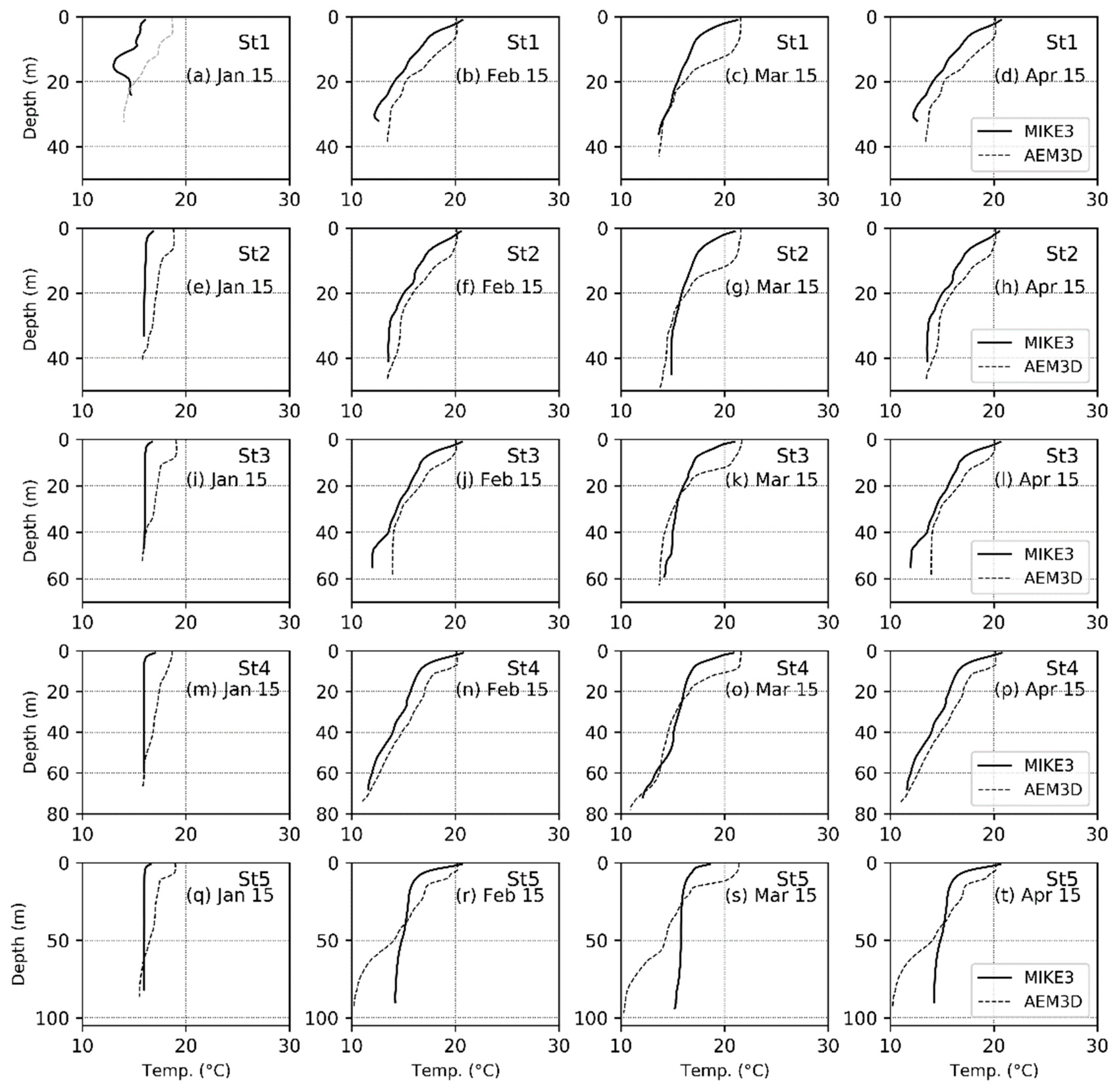
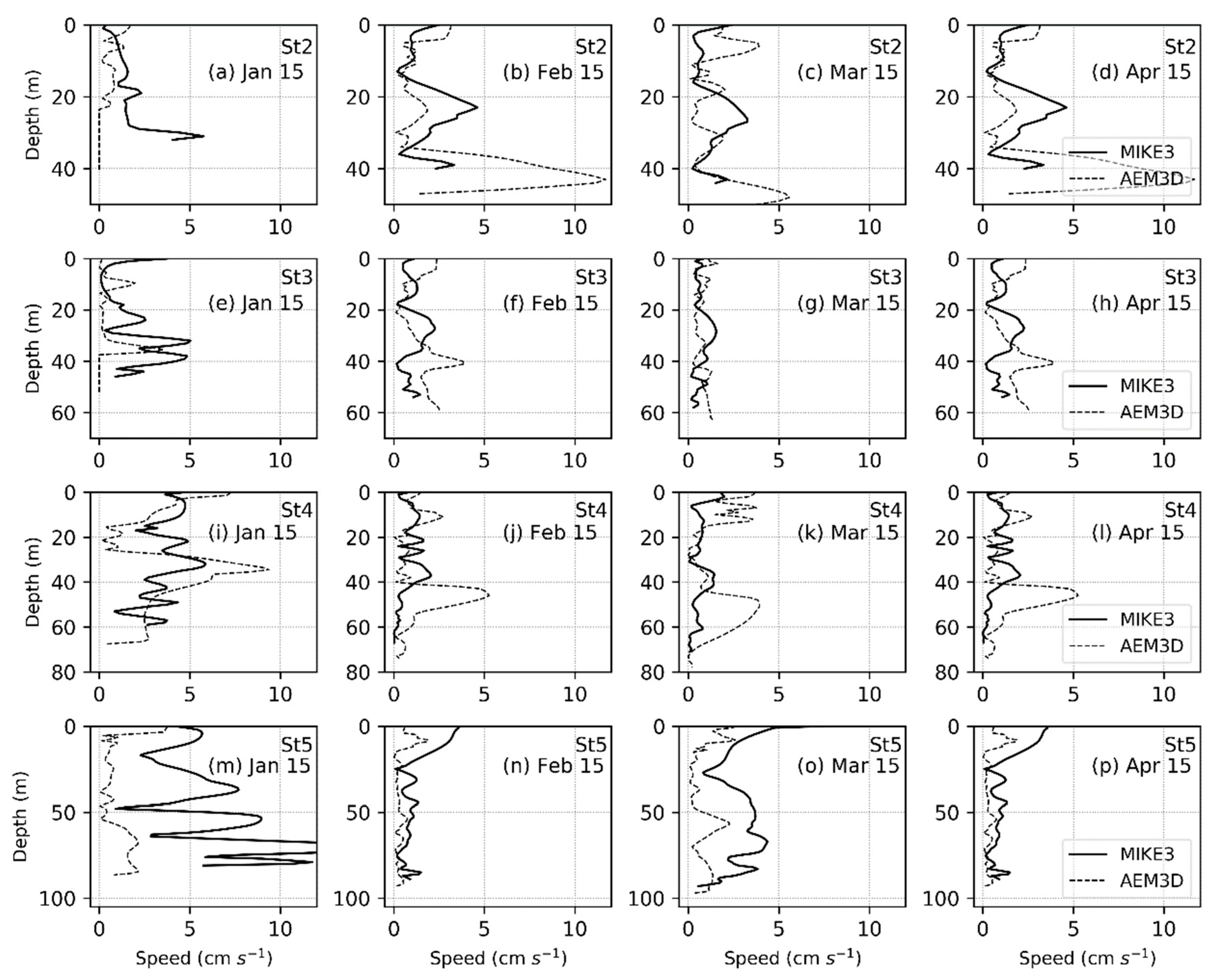
Figure 8 and Figure 9 show the single station water temperature and current speed profiles, respectively, simulated by the two models. Both models capture the winter mixing and the spring stratification development at different stages more or less equally well, as the entire water column temperatures from surface to bottom are consistently well simulated by the two models. However, some degree of underestimation is seen in the MIKE3-simulated surface mixed layer temperatures again. In other words, MIKE3 is unable to simulate the surface wind-mixed layer which extends up to several meters in depth, unlike AEM3D. Although the absence of measured vertical water temperature profiles in the Maroon Reservoir limits us in comparing the surface mixed layer exactly in the study location, a similar presence of this surface mixed layer in reservoirs near the present Maroon Reservoir [58], and the good capability of AEM3D in precisely capturing the mixed layer depth, has been shown in the literature [9,11,59]. Based on these results, we are confident that AEM3D is capable of simulating the wind-mixed layer in the Maroon Reservoir in a reliable manner as well.
The inconsistency in simulating the wind-mixed layer depth between the two models is very likely due to the poor introduction of wind stress momentum at the reservoir’s surface boundary, which can happen for several reasons, depending on the vertical mixing model. As mentioned in Section 2.5.1, the vertical mixing in MIKE3 is formulated using either a constant eddy viscosity or a k-ε model. These formulations strongly depend on the empirical values of the eddy viscosity and diffusivity which normally need calibration. In fact, such a calibration was performed by Rodi [47], and his “best” values for eddy viscosity and diffusivity, listed in Table 2, have been accepted in most modeling studies since then and are also recommended by DHI [19]. In stratified systems, the depth, downwind velocity and velocity shear in the wind-mixed layer are highly dependent on the values of these two coefficients above the thermocline. Therefore, the prediction of the mixed-layer depth requires, on one hand, fine grid resolutions, whereas, on the other hand, it is shown by [9] and [60] that k-ε models may not be capable of mimicking the rigorous dynamics of the wind-mixed layer, even at fine resolutions. Therefore, it can be concluded that the better representation of the wind-mixed layer by AEM3D than by MIKE3 is the result of the substitution of the “free” and uncertain eddy viscosity term in MIKE3 by the use of a standalone 3D vertical mixing model in AEM3D which predicts the wind-mixed layer depth and the distribution of momentum over depth better [9], while at the same time obviating the need for very fine resolutions to represent the wind-mixed layer appropriately.
3.2. Water Column Profiles
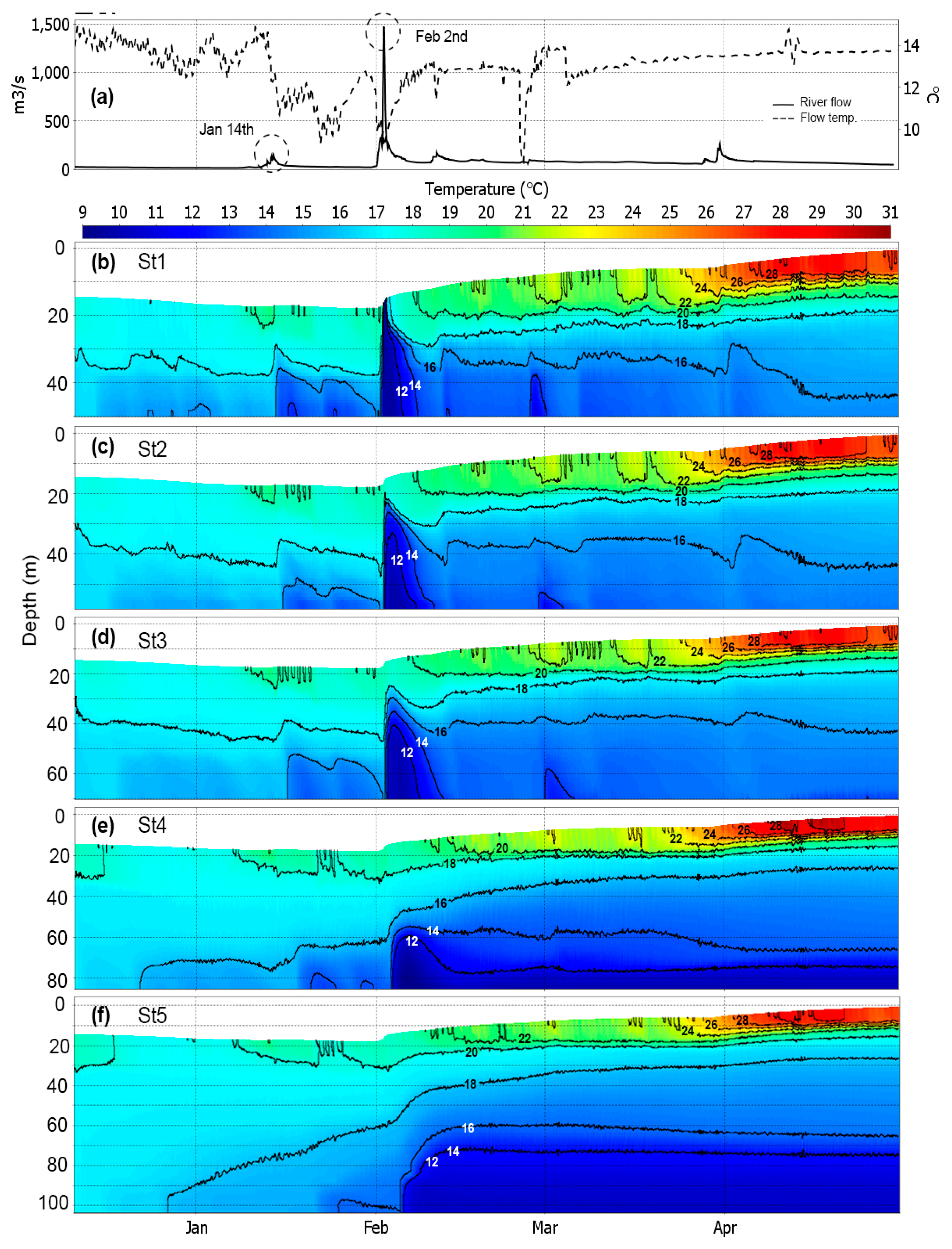
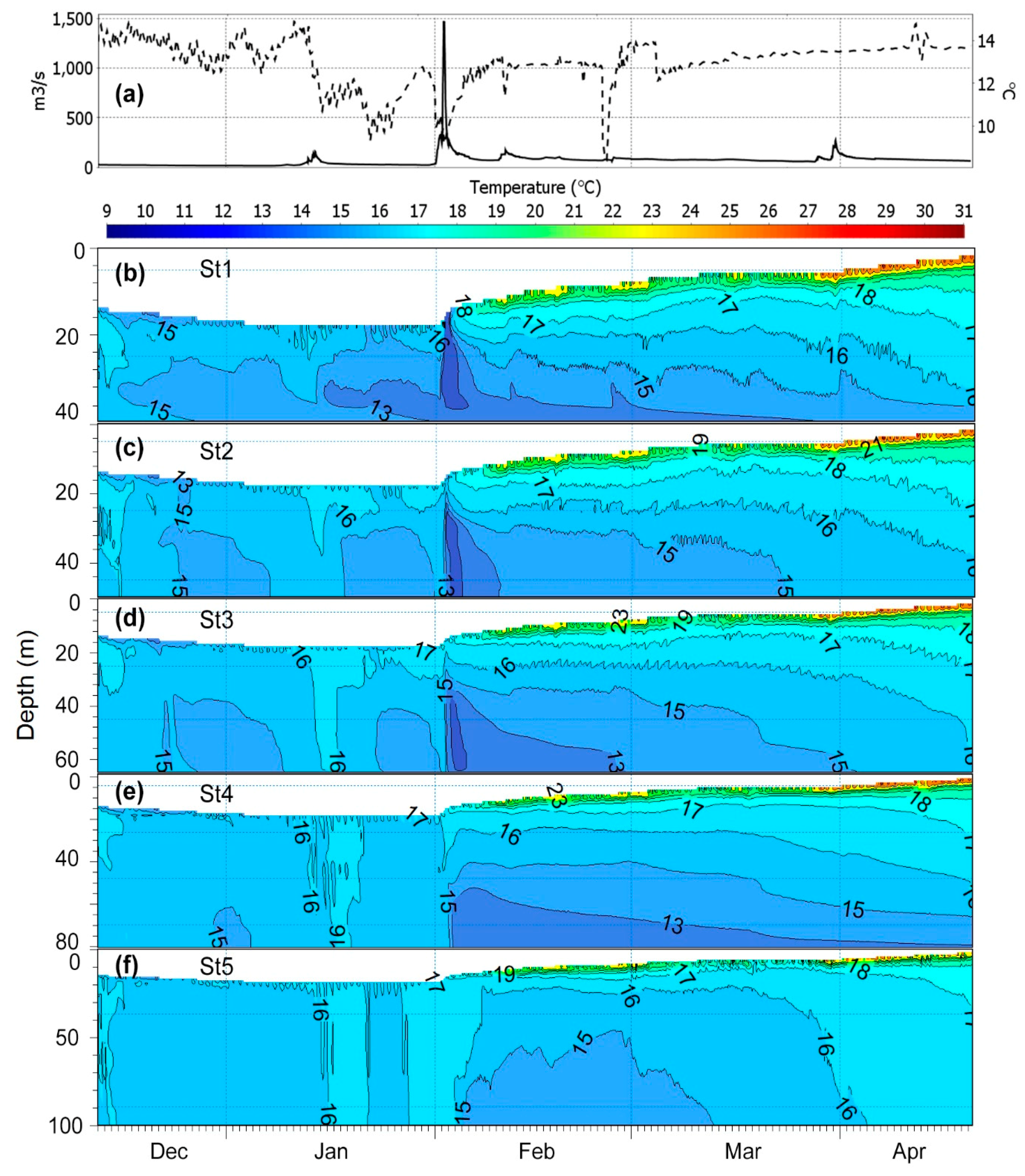
Continuous depth profiles of water temperature simulated by AEM3D and MIKE3 are shown in Figure 10 and Figure 11, respectively. Generally, AEM3D reproduces the various observed characteristics of the transient temperature field evolution in the reservoir better than MIKE3. For example, unlike the former, the latter is not capable of properly simulating the formation of the cold bottom layer after the propagation of the February 2 large cold flood. Thus, the rapid fall of the water temperature in the wake of the cold flood bore is simulated better by AEM3D than by MIKE3; as for the latter, nearly no signal of that cold current is seen in the downstream basin of the reservoir (Figure 10f), unlike for AEM3D (Figure 11f), for which it is well pronounced.
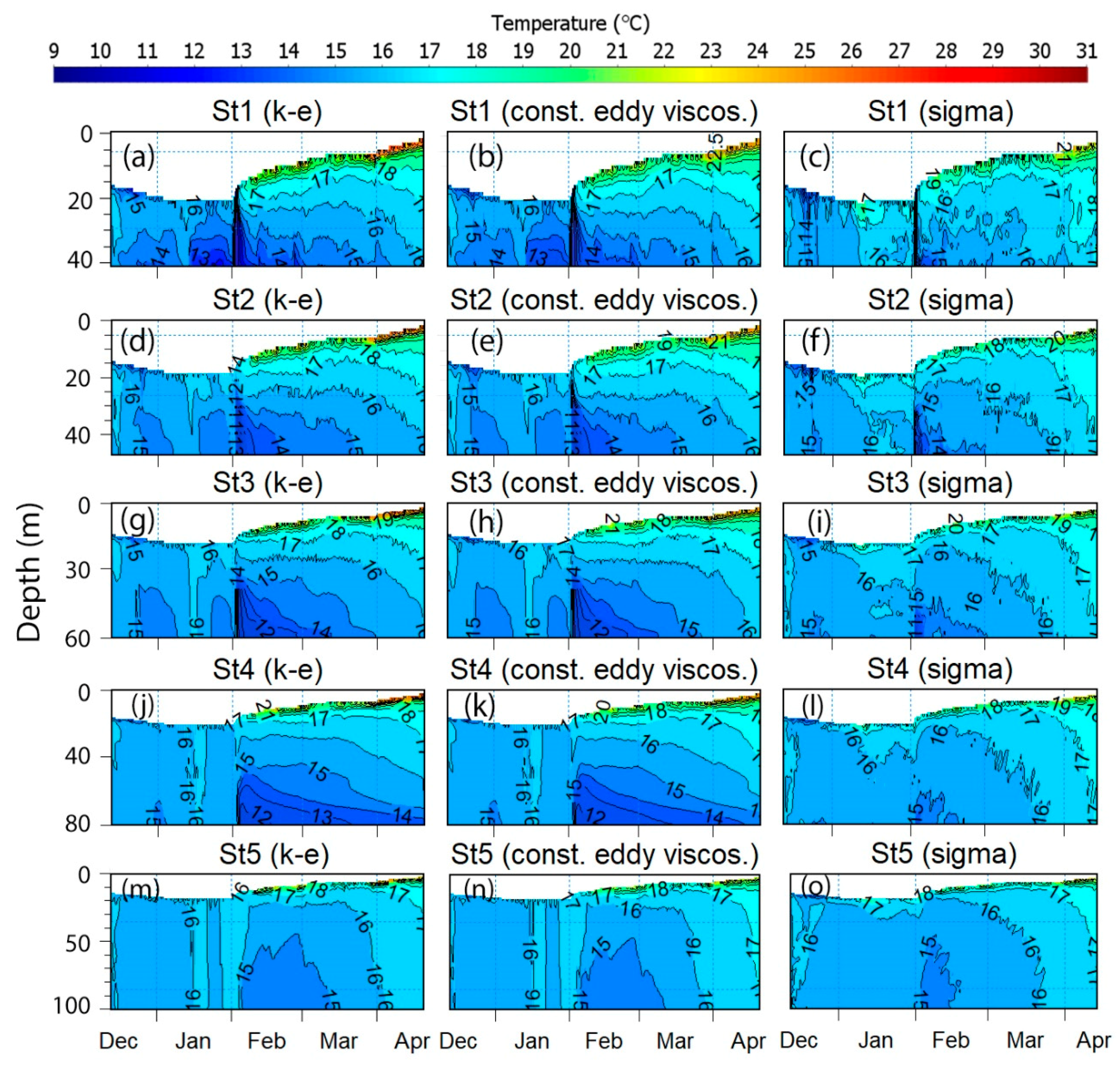
The overall poorer performance of MIKE3 than AEM3D is likely due to the different bathymetry representation in the two models, as the poor performance of MIKE3 can be seen within all its three vertical discretizations and turbulence models (discussed in Table 4) (Figure 12). For example, the coarse MIKE3 grid size does not allow an accurate representation of the river channel and the thalweg in the reservoir, particularly, in the upstream narrow valleys and in the canyon connecting the up- and downstream basins. Although the flexible mesh (FM) option in MIKE3 made it possible, to some extent, to define a finer discretization in these narrow parts of the reservoir, a finer grid size yet seems to be necessary here to resolve the bottom boundary layers within the sigma domain to satisfy the “hydrostatic consistency” condition [46] and, so, to produce smaller errors. However, such a finer grid size would result in unacceptably long simulation runs, which are not feasible with the computing resources available to us. Overall, MIKE3 appears to need a finer grid than AEM3D to reproduce a similar degree of accuracy and to capture the details of the propagation of the cold flood (density) currents within the reservoir.
The use of the sigma and/or z-sigma vertical discretizations in MIKE3, when compared with the purely z-level discretization of AEM3D, is likely another reason for the need of a finer grid size. In a steep topography (e.g., steep walls of a reservoir), the sigma-discretization generates significant errors by under/overestimating the baroclinic pressure terms and the sharp density gradients [45,57] that leads to the well-known horizontal pressure, scalar concentration and velocity gradient errors [46] which, in total, increase the model error (see Table 3).
3.3. General Error Discussion
3.3.1. Effect of Poor Grid-Size Resolution
It must be noted that the two models’ results represent the average water temperature (and other variables) of the entire cell (size of 100 × 100 m area in AEM3D and a varying area size in MIKE3), while the measurements are recorded at the corresponding (x, y, z) coordinate of the sensor. Therefore, some discrepancies between the simulated and observed datasets are to be expected. However, the main cause of the named minor discrepancies between model and observations is the poor representation of the reservoir’s thalweg and of the overall geometry of the model grid. The geometry influences the dynamics of internal waves, transport and representation of the thermal cycle, thereby introducing a range of error sources. This is a common challenging modeling problem in reservoirs with complex morphometry [9]. In particular, Maroon Reservoir’s thalweg is a narrow V-shaped valley with steep slopes in most sections, especially in the riverine and transition zones, with the bottom of the real thalweg being typically narrower than the grid size (see Figure 3). Due to the steep slopes, the model grid size remains wider than the real thalweg up to several or, at some places, tens of meters above the bottom. This translates into a diminishing of the kinetic energy and excessive mixing of the propagating currents in the bottom of the mostly wider thalweg of the model when compared with the real one.
3.3.2. Effect of Hydrostatic Model Assumption
Hodges et al. [53] showed that another part of the model-observation discrepancies arises from the hydrostatic approximation assumed in both models which neglects the small-scale (relative to the hydrostatic pressure gradient) non-hydrostatic pressure gradients in the internal waves, while the nonlinear effects are still preserved. Because of this neglect, the internal waves steepen and show a temporal horizon, or what is called a steepening time scale. The latter is a fundamental problem phenomenon when using the hydrostatic approximation and cannot be removed by a pure model grid refinement. However, despite this grain of salt, we are confident that both models simulate the observed temporal water temperature variations for all stations reasonably well. Thus, the overall five-month trends and characteristic of simulations and observations are similar, with key events occurring at comparable scales and timing (e.g., rapid cooling in February seen in Figure 6 and Figure 7). The agreement seems to be higher in the upstream rather than downstream zones of the reservoir (see Table 3), which is also noticeable from the lower correlations between simulated and observed data at the downstream stations (Table 4). The downstream increase of the error is likely due to (i) the net downstream transport of the temperature, which is inherently accumulative over the residence time of the reservoir, as is the error; (ii) the incorrect modeling of the mixing processes and the energy balance in the sloping boundaries of the reservoir; and (iii) nonrepresentation of the non-hydrostatic effects in the internal waves in the two hydrostatic models used here [9].
4. Conclusions
Our study shows that both AEM3D and MIKE3 models simulate the hydrodynamics of the Maroon Reservoir with errors in a reasonable range and the results are not significantly different from the observed data. However, AEM3D showed a performance better than MIKE3 in our studied reservoir. Depending on the vertical mixing model and the discretization method, MIKE3 generated errors from 59% to 100% larger than those of AEM3D. The error values in both models, especially in MIKE3, increased in downstream stations, which is mainly because of the accumulation of the errors that are generated by the representation of bathymetry with a coarse resolution. This translates into a higher dissipation of the propagating currents upstream and more mixing in the reservoir which results in overestimation of temperature in downstream locations. We found that the 3D vertical mixing model in AEM3D [9], used instead of the constant vertical eddy viscosity and k-ε turbulence model formulations, more precisely models the surface wind-mixed layer depth than the eddy viscosity and k-ε approaches used in MIKE3.
This paper is a first step to evaluate and study the capability of the MIKE3 model in simulating reservoirs. The performance of the MIKE3 model was examined under different model discretization approaches and turbulence model configurations, of which the best results (smallest errors) were seen by the k-ε model with z-sigma hybrid vertical discretization. Of the two possible vertical discretization methods of MIKE3, the sigma-only discretization generated the poorest results with errors 35%–46% larger than those of the z-sigma hybrid discretization of same grid size. These results indicate the weakness of the sigma discretization in the reservoirs with steep topography.
Although a smaller grid size was defined in the narrow valleys than in the wider downstream lacustrine zone in MIKE3’s model grid, the complex and steep bathymetry of these locations is not yet captured well. Even using the z-sigma hybrid vertical discretization, these steep walls still exist within the sigma domain and the boundary between the two domains, as shown by [27], which result in excess errors. These errors were not generated by the completely Cartesian z-coordinate grid in AEM3D, and its stair-like vertical discretization seems better in representing these complexities with considerably smaller errors. Therefore, the AEM3D model, with its inherent features for simulating reservoirs, proved to be a better model to simulate reservoirs with steep boundaries and noticeable water level fluctuations.
Another restriction of MIKE3 that emerged during this study, was the weakness of bathymetry interpolation by the Mesh Generator tool in MIKE3. In the sections of the river where the longitudinal bed slope is not very steep and contours are far from each other, this tool is not able to rigorously interpolate and represent the thalweg slope in the river valley from the bathymetry data. Moreover, we found that further manipulations of the grid to correct these unrealistic slopes (after generating the mesh) would result in unknown model instabilities, which needs further investigation.
Resolving the complex bathymetry of narrow and steep sections in the Maroon Reservoir using the flexible mesh of MIKE3 typically needs a higher resolution than the other locations. This high resolution requires smaller time steps at these cells, leading to significantly higher simulation times. On the same computational platform, MIKE3 requires a roughly 70% longer simulation time than AEM3D with a nearly similar average grid size.
By comparing these two models, we found AEM3D as a more appropriate model for simulating reservoirs with complex bathymetry and steep walls. Any further use of MIKE3 on such reservoirs requires improvements in this model code to better introduce the reservoir-specific boundary conditions and prepare it for simulating such complex bathymetries while preserving the simulation time. We also add that MIKE3 is not tested for natural lakes or reservoirs with simple bathymetry, and it may perform better in such cases than the case of this study, which still needs to be studied.
Author Contributions
Conceptualization, B.Z. and M.K.; methodology, B.Z. and M.K; software and models, B.Z.; validation, B.Z.; formal analysis, B.Z.; investigation, B.Z. and M.K; writing—original draft preparation, B.Z.; writing—review and final editing, M.K.; visualization, B.Z.; supervision, M.K.; project administration, B.Z. All authors have read and agreed to the published version of the manuscript.
Funding
This research received no external funding.
Acknowledgments
The MIKE3 model was provided by the Danish Hydraulic Institute (DHI) as an academic license for this study. We appreciate the Iranian Meteorological Organization for supporting us with the meteorological data and Mr. Ali Mohammadi Ahari (Iranian Ministry of Energy) for kindly providing the river flow data. We also thank Mehdi Ghomeshi for his valuable advice and information regarding the Maroon River and Reservoir. We also thank the anonymous reviewers who provided helpful and constructive comments and suggestions to improve our manuscript.
Conflicts of Interest
The authors declare no conflict of interest.
References
- USACE. Reservoir Water Quality Analysis, Engineer Manual; U.S. Army Corps of Engineers: Washington, DC, USA, 1987. [Google Scholar]
- Hamilton, D.P.; Schladow, S.G. Prediction of water quality in lakes and reservoirs: Part I-Model description. Ecol. Modell. 1997, 96, 91–110. [Google Scholar] [CrossRef]
- Schladow, S.G.; Hamilton, D.P. Prediction of water quality in lakes and reservoirs: Part II-Model calibration, sensitivity analysis and application. Ecol. Modell. 1997, 96, 111–123. [Google Scholar] [CrossRef]
- Löffler, H. The origin of lake basins. In The Lakes Handbook, 2nd ed.; O’Sullivan, P.E., Reynolds, C.S., Eds.; Blackwell Publishing: Oxford, UK, 2004; Volume 1, pp. 8–60. [Google Scholar]
- Ji, Z.-G. Hydrodynamics and Water Quality: Modeling Rivers, Lakes, and Estuaries, 1st ed.; John Wiley & Sons, Inc.: Hoboken, NJ, USA, 2008. [Google Scholar]
- Valerio, G.; Pilotti, M.; Marti, C.L.; Imberger, J. The structure of basin-scale internal waves in a stratified lake in response to Lake Bathymetry and wind spatial and temporal distribution: Lake Iseo, Italy. Limnol. Oceanogr. 2012, 57, 772–786. [Google Scholar] [CrossRef]
- Boegman, L.; Imberger, J.; Ivey, G.N.; Antenucci, J.P. High-frequency internal waves in large stratified lakes. Limnol. Oceanogr. 2003, 48, 895–919. [Google Scholar] [CrossRef]
- Marti, C.L.; Imberger, J. Dynamics of the benthic boundary layer in a strongly forced stratified lake. J. Hydrobiol. 2006, 568, 217. [Google Scholar] [CrossRef]
- Hodges, B.R.; Imberger, J.; Saggio, A.; Winters, K.B. Modeling basin-scale internal waves in a stratified lake. Limnol. Oceanogr. 2000, 45, 1603–1620. [Google Scholar] [CrossRef] [Green Version]
- Laval, B.; Imberger, J.; Hodges, B.R.; Stocker, R. Modeling circulation in lakes: Spatial and temporal variations. Limnol. Oceanogr. 2003, 48, 983–994. [Google Scholar] [CrossRef] [Green Version]
- Zamani, B.; Koch, M.; Hodges, B.R.; Fakheri-Fard, A. Pre-impoundment assessment of the limnological processes and eutrophication in a reservoir using three-dimensional modeling: Abolabbas reservoir, Iran. J. Appl. Water Eng. Res. 2018, 6, 48–61. [Google Scholar] [CrossRef]
- Pacanowski, R.C.; Dixon, K.W.; Rosati, A.J. The GFDL Modular Ocean Model Users Guide (Technical Report); GFDL Ocean Group NOAA/Geophysical Fluid Dynamics Laboratory: Princeton, NJ, USA, 1991.
- Cassulli, V.; Cheng, R.T. Semi-implicit finite difference methods for three-dimensional shallow water flow. Int. J. Numer. Methods 1992, 15, 629–648. [Google Scholar] [CrossRef]
- Hodges, B.R.; Dallimore, C. Aquatic Ecosystem Model: AEM3D, User Manual; Hydronumerics: Docklands, Australia, 2016. [Google Scholar]
- Phillips, N.A. A coordinate system having some special advantage for numerical forecasting. J. Meteorol. 1957, 14, 184–185. [Google Scholar] [CrossRef] [Green Version]
- Blumberg, A.F.; Mellor, G.L. A description of a three-dimensional coastal ocean circulation model. In Coastal Estuarine Science. 4. Three Dimensional Coastal Ocean Models; Heaps, N., Ed.; American Geophysical Union: Washington, DC, USA, 1987; pp. 1–16. [Google Scholar]
- Haidvogel, D.B.; Wilkin, J.L.; Young, R.E. A semi-spectral primitive equation ocean circulation model using vertical sigma and orthogonal curvilinear horizontal co-ordinates. J. Comput. Phys. 1991, 94, 151–185. [Google Scholar] [CrossRef]
- Hamrick, J.M. A Three-Dimensional Environmental Fluid Dynamics Computer Code: Theoretical and Computational Aspects. Special Report. No. 317; The College of William and Mary, Virginia Institute of Marine Science: Gloucester Point, VA, USA, 1991. [Google Scholar]
- DHI. MIKE3 Flow Model FM Hydrodynamic and Transport Module, Scientific Documentation; DHI Danish Hydraulic Institute: Hørsholm, Denmark, 2017. [Google Scholar]
- Pierrzak, J.; Jakobson, J.B.; Burchard, H.; Vested, H.J.; Petersen, O. A three-dimensional hydrostatic model for coastal and ocean modelling using a generalised topography following co-ordinate system. Ocean Modell. 2002, 4, 173–205. [Google Scholar] [CrossRef]
- Gerdes, R. A primitive equation ocean circulation model using a general vertical coordinate transformation: 2. Application to an overflow problem. J. Geophys. Res. 1993, 98, 14703–14726. [Google Scholar] [CrossRef]
- Bell, M.J. Vortex stretching and bottom torques in the Bryan-Cox ocean circulation model. J. Geophys. Res. 1999, 104, 23545–23563. [Google Scholar] [CrossRef]
- Bleck, R.; Boudra, D. Initial testing of a numerical ocean circulation model using a hybrid (quasi-isopycnic) vertical coordinate. J. Phys. Oceanogr. 1981, 11, 755–770. [Google Scholar] [CrossRef] [Green Version]
- Bleck, R.; Benjamin, S. Regional weather prediction with a model combining terrain-following and isentropic coordinates. Part I: Model description. Mon. Weather Rev. 1993, 121, 1770–1785. [Google Scholar] [CrossRef] [Green Version]
- Mellor, G.L.; Häkkinen, S.; Ezer, T.; Patchen, R. A generalization of a sigma coordinate ocean model and an intercomparison of model vertical grids. In Ocean Forecasting: Theory and Practice; Pinardi, N., Ed.; Springer: Berlin, Germany, 1999. [Google Scholar]
- Burchard, H.; Petersen, O. Hybridization between σ- and z-co-ordinates for improving the internal pressure gradient calculation in marine models with steep bottom slopes. Int. J. Numer. Methods Fluids 1997, 25, 1003–1023. [Google Scholar] [CrossRef]
- Zhang, Y.J.; Ateljevich, E.; Yu, H.; Wu, C.H.; Yu, J.C.S. A new vertical coordinate system for a 3D unstructured-grid model. Ocean Modell. 2015, 85, 16–31. [Google Scholar] [CrossRef]
- Craig, P.M.; Chung, D.H.; Lam, N.T.; Son, P.H.; Tinh, N.X. Sigma-zed: A computationally efficient approach to reduce the horizontal gradient error in the EFDC’s vertical sigma grid. In Proceedings of the 11th International Conference on Hydrodynamics (ICHD 2014), Singapore, 19–24 October 2014. [Google Scholar]
- Ford, D.E.; Johnson, L.S. An Assessment of Reservoir Mixing Processes, Technical Report for US Army Corps of Engineers; Ford Thornton Norton and associates Ltd.: Little Rock, AR, USA, 1986. [Google Scholar]
- Hutchinson, G.E.; Löffler, H. The thermal classification of lakes. Proc. Natl. Acad. Sci. USA 1956, 42, 84–86. [Google Scholar] [CrossRef] [Green Version]
- Wüest, A.; Lorke, A. Small-scale hydrodynamics in lakes. Annu. Rev. Fluid Mech. 2003, 35, 373–412. [Google Scholar] [CrossRef]
- Karandish, F.; Porhemmat, J.; Ebrahimi, K. Determination of the main snowmelt parameters in estimating flood hydrograph in Karun basin. Iran Water Res. J. 2016, 10, 133–142. [Google Scholar]
- Allen, R.G.; Pereira, L.S.; Raes, D.; Smith, M. Crop Evapotranspiration – Guidelines for Computing Crop Water Requirements. FAO Irrigation and Drainage Paper 56; Food and Agriculture Organization of the United Nations (FAO): Rome, Italy, 1998. [Google Scholar]
- Kamali, G.; Moradi, E. Solar Radiation (Principles and Applications in Agriculture and New Energies); Atmospheric Science and Meteorological Research Center: Tehran, Iran, 2006. (In Persian) [Google Scholar]
- Alizadeh, A.; Khalili, N. Estimation of Angstrom coefficient and developing a regression equation for solar radiation estimation (case study: Mashhad). J. Water Soil 2009, 23, 229–238. (In Persian) [Google Scholar]
- Yang, K.; Koike, T. A general model to estimate hourly and daily solar radiation for hydrological studies. Water Resour. Res. 2005, 41, W10403. [Google Scholar] [CrossRef] [Green Version]
- Hajjam, S.; Jamei, M. Estimation of solar radiation parameter (sunshine hours) and Angstrom coefficients in Khuzestan Province. In Proceedings of the 10th National Conference of Irrigation and Evaporation Reduction, Kerman, Iran, 8 February 2009. (In Persian). [Google Scholar]
- Mehrabani, R.; Makvandi, A.; Nekouyanfar, M.; Hassounizadeh, H. Tracing and measurement of turbidity current in maroon dam. In Proceedings of the 9th International River Engineering Conference, Ahwaz, Iran, 13–15 February 2013. [Google Scholar]
- Hodges, B.R. Numerical Tecniques in CWR-ELCOM, Technical Report; Center for Water Research, The Univerity of Western Australia: Nedlands, Australia, 2000. [Google Scholar]
- Hipsey, M.R.; Romero, J.R.; Antenucci, J.J.; Hamilton, D. Computational Aquatic Ecosystem Dynamics Model: CAEDYM v3.2, Science Manual; Centre for Water Research, University of Western Australia: Nedlands, Australia, 2006. [Google Scholar]
- Arakawa, A.; Lamb, V.R. Computational design of the basic dynamical processes of the UCLA general circulation model In General Circulation Models of the Atmosphere. Methods Comput. Phys. 1977, 17, 173–265. [Google Scholar]
- Imberger, J.; Patterson, J.C. A dynamic reservoir simulation model—DYRESM: 5. In Transport Models for Inland and Coastal Waters; Fischer, H.B., Ed.; Academic Press: Cambridge, MA, USA, 1981; pp. 310–361. [Google Scholar]
- Imberger, J.; Patterson, J.C. Physical limnology. Adv. Appl. Mech. 1990, 27, 303–475. [Google Scholar]
- Spigel, R.H.; Imberger, J. The classification of mixed layer dynamics in lakes of small to medium size. J. Phys. Oceanogr. 1980, 10, 1104–1121. [Google Scholar] [CrossRef] [Green Version]
- Haney, R.L. On the pressure gradient force over steep topography in sigma co-ordinate ocean models. J. Phys. Oceanogr. 1991, 21, 610–619. [Google Scholar] [CrossRef] [Green Version]
- Mellor, G.L.; Ezer, T.; Oey, L. The Pressure Gradient Conundrum of Sigma Coordinate Ocean Models. J. Atmos. Ocean. Technol. 1994, 11, 1126–1134. [Google Scholar] [CrossRef] [Green Version]
- Rodi, W. Turbulence Models and Their Applications in Hydraulics. IAHR Monograph, 2nd ed.; CRC Press: Boca Raton, FL, USA, 1984. [Google Scholar]
- Lange, X. Numerical Simulations of Estuarine Circulation in a Non-Tidal Estuary. Master’s Thesis, University of Rostock, Rostock, Germany, 2015. [Google Scholar]
- Sikirić, M.D.; Janeković, I.; Kuzmić, M. A new approach to bathymetry smoothing in sigma-coordinate ocean models. Ocean Modell. 2009, 29, 128–136. [Google Scholar] [CrossRef]
- Chung, S.W.; Hipsey, M.R.; Imberger, J. Modelling the propagation of turbid density inflows into a stratified lake: Daecheong Reservoir, Korea. Environ. Modell. Softw. 2009, 24, 1467–1482. [Google Scholar] [CrossRef]
- Marti, C.L.; Imberger, J.; Garibaldi, L.; Leoni, B. Using time scales to characterize phytoplankton assemblages in a deep subalpine lake during the thermal stratification period: Lake Iseo, Italy. Water Resour. Res. 2016, 52, 1762–1780. [Google Scholar] [CrossRef]
- Lee, H.W.; Kim, E.J.; Park, S.S.; Choi, J.H. Effects of Climate Change on the Movement of Turbidity Flow in a Stratified Reservoir. Water Resour. Manag. 2015, 29, 4095–4110. [Google Scholar] [CrossRef]
- Hodges, B.R.; Laval, B.; Wadzuk, B.M. Numerical error assessment and a temporal horizon for internal waves in a hydrostatic model. Ocean Modell. 2006, 13, 44–64. [Google Scholar] [CrossRef]
- Lindim Fontes, C. Modelling of Water Quality in the Alqueva Reservoir, Portugal. Ph.D. Thesis, University of Minho, Braga, Portugal, 2010. [Google Scholar]
- Ji, Z.G.; Hu, G.; Shen, J.; Wan, Y. Three-dimensional modeling of hydrodynamic processes in the St. Lucie Estuary. Estuar. Coast. Shelf Sci. 2007, 73, 188–200. [Google Scholar] [CrossRef]
- Launder, B.; Spalding, D. Mathematical Models of Turbulence; Academic Press: Cambridge, MA, USA, 1972. [Google Scholar]
- Gary, J.M. Estimate of truncation error in transformed co-ordinate, primitive equation atmospheric models. J. Atmos. Sci. 1973, 30, 223–233. [Google Scholar] [CrossRef] [Green Version]
- Salimi-Nasab, S.; Espandar, R.; Zandi, R. Assessment of thermal stratification and oxygen distribution in Karkheh dam reservoir. In Proceedings of the 2nd Iranian National Conference on Dams and Hydropower, Tehran, Iran, 14 May 2008. [Google Scholar]
- Paturi, S.; Boegman, L.; Yerubandi, R.R. Hydrodynamics of eastern Lake Ontario and the upper St. Lawrence River. J. Great Lakes Res. 2012, 38 (Suppl. 4), 194–204. [Google Scholar] [CrossRef]
- Martin, P.J. Simulation of the mixed layer at OWS November and Papa with several models. J. Geophys. Res. 1985, 90, 903–916. [Google Scholar] [CrossRef]
Figure 1.
(a) Orientation map of the Maroon Reservoir; (b) Maroon Reservoir catchment and location of the Behbahan synoptic and Eydanak rain gauge stations; (c) Maroon Reservoir bathymetry and sensor locations.
Figure 1.
(a) Orientation map of the Maroon Reservoir; (b) Maroon Reservoir catchment and location of the Behbahan synoptic and Eydanak rain gauge stations; (c) Maroon Reservoir bathymetry and sensor locations.

Figure 2.
(a) AEM3D model grid; (b) MIKE3 model grid.

Figure 3.
(a) Inflow boundary of MIKE3. The gray line in the background outlines the boundary of the AEM3D grid for comparison. (b) Inflow boundary of AEM3D with meandering inflow boundary. The black arrows show the direction of the inflow at each cell of the inflow boundary (under the “flow_multi_sides” feature).

Figure 4.
Simulation errors AME (a) and RMSE (b) for AEM3D and MIKE3.

Figure 5.
Observed and AEM3D- and MIKE3-simulated Maroon Reservoir water levels over the five-month simulation period. The color band illustrates the range of ±standard deviation of the observed water levels.
Figure 5.
Observed and AEM3D- and MIKE3-simulated Maroon Reservoir water levels over the five-month simulation period. The color band illustrates the range of ±standard deviation of the observed water levels.

Figure 6.
Observed (red dashed) and simulated water temperature using AEM3D (black) and MIKE3 with k-ε vertical discretization (blue dashed) versus measured values for the five gauging stations. All water temperatures are taken at sensor depths (2 m above bottom). Light red bands indicate the range of the ±standard deviation of the measured data. The red band at St5 is intentionally not indicated, as the observed data of St5 represent a shorter period (from February) than other stations.

Figure 7.
MIKE3-simulated water temperature using different discretizations and vertical mixing models: z-sigma with k-ε turbulence model (blue), z-sigma with constant eddy viscosity (green) and sigma k-ε turbulence model (red) versus measured values (dashed) at measurement depths of each station. Light red bands delineate the range of the ±standard deviation of the measured data. The red band at St5 is intentionally not indicated as the observed data of St5 represent a shorter period (from February) than other stations.

Figure 8.
Comparison between MIKE3 (continuous lines) and AEM3D (dashed lines) water temperature profiles simulated at different times and different locations of the Maroon Reservoir.
Figure 8.
Comparison between MIKE3 (continuous lines) and AEM3D (dashed lines) water temperature profiles simulated at different times and different locations of the Maroon Reservoir.

Figure 9.
Comparison between MIKE3 (continuous lines) and AEM3D (dashed lines) simulated current speed profiles at different times and locations of the Maroon Reservoir.
Figure 9.
Comparison between MIKE3 (continuous lines) and AEM3D (dashed lines) simulated current speed profiles at different times and locations of the Maroon Reservoir.

Figure 10.
(a) River flow rate (continuous line) and temperature (dashed line) in the Maroon Reservoir; (b–f) temporal variation of AEM3D-simulated water column temperatures at the various measurement stations.
Figure 10.
(a) River flow rate (continuous line) and temperature (dashed line) in the Maroon Reservoir; (b–f) temporal variation of AEM3D-simulated water column temperatures at the various measurement stations.

Figure 11.
Similar to Figure 10, but with water column temperatures simulated by MIKE3 (k-ε) using z/sigma discretization.
Figure 11.
Similar to Figure 10, but with water column temperatures simulated by MIKE3 (k-ε) using z/sigma discretization.

Figure 12.
Temporal variations of the simulated water temperature by MIKE3 with different model discretizations and turbulence models as profiles of water column temperature at measurement locations in the Maroon Reservoir.
Figure 12.
Temporal variations of the simulated water temperature by MIKE3 with different model discretizations and turbulence models as profiles of water column temperature at measurement locations in the Maroon Reservoir.


Table 1.
Parameters used in the AEM3D simulations.
| Parameter | Description | Unit | Value |
|---|---|---|---|
| CD | Bottom drag coefficient | - | 0.05 |
| λPAR | Light extinction coefficient | m−1 | 0.25 |
| αsw | Mean albedo for short-wave radiation | - | 0.08 |
| αlw | Mean albedo for long-wave radiation | - | 0.03 |
| Cd | Wind stress coefficient | - | 0.0013 |
| CH/S | Bulk-transfer constant for surface scalar fluxes | - | 0.013 |
Table 2.
Parameters used in the MIKE3 simulations.
| Parameter | Description | Unit | Value |
|---|---|---|---|
| Vertical eddy viscosity of k-ε model | m2 s−1 | 1 × 10⁻⁶ to 1 × 10⁻⁵ | |
| Horizontal eddy viscosity | m2 s−1 | 0.002 | |
| Wind stress coefficient | - | 0.0013 | |
| Bottom drag coefficient (bed resistance) | - | 0.055 | |
| Horizontal diffusion coefficients | - | 0.002, 0.0015 | |
| Vertical diffusion coefficient | - | 1.1 × 10⁻⁶ |
Table 3.
Statistical results of AEM3D and MIKE3 (with different grid and vertical mixing models).
| Model | Station | Mean (obs) (°C) | Mean (sim) (°C) | AME (°C) | RMSE (°C) |
|---|---|---|---|---|---|
| AEM3D | St1 | 14.27 | 14.96 | 0.82 | 0.97 |
| St2 | 14.57 | 14.48 | 0.41 | 0.71 | |
| St3 | 14.59 | 14.97 | 0.65 | 0.81 | |
| St4 | 14.19 | 13.98 | 0.88 | 1.07 | |
| St5 | 13.05 | 13.08 | 0.71 | 0.91 | |
| Mean | 0.70 | 0.89 | |||
| MIKE3 z-sigma k-ε | St1 | 14.27 | 14.20 | 0.71 | 0.90 |
| St2 | 14.57 | 14.60 | 0.96 | 1.16 | |
| St3 | 14.59 | 14.85 | 0.90 | 1.04 | |
| St4 | 14.19 | 13.87 | 0.79 | 1.02 | |
| St5 | 13.05 | 15.20 | 2.65 | 2.83 | |
| Mean | 1.20 | 1.39 | |||
| MIKE3 z-sigma eddy viscosity | St1 | 14.27 | 14.43 | 0.80 | 0.99 |
| St2 | 14.57 | 15.09 | 1.05 | 1.25 | |
| St3 | 14.59 | 15.22 | 1.13 | 1.27 | |
| St4 | 14.19 | 14.10 | 0.97 | 1.10 | |
| St5 | 13.05 | 15.32 | 2.82 | 3.01 | |
| Mean | 1.35 | 1.52 | |||
| MIKE3 sigma k-ε | St1 | 14.27 | 15.29 | 1.02 | 1.32 |
| St2 | 14.57 | 15.59 | 1.38 | 1.66 | |
| St3 | 14.59 | 15.21 | 1.28 | 1.48 | |
| St4 | 14.19 | 15.74 | 2.31 | 2.54 | |
| St5 | 13.05 | 15.79 | 3.13 | 3.23 | |
| Mean | 1.83 | 2.05 |
Table 4.
Correlations between models and measured data at different stations.
| Station | AEM3D | MIKE3 z-sigma k-ε | MIKE3 z-sigma eddy viscosity | MIKE3 sigma k-ε |
|---|---|---|---|---|
| St1 | 0.90 | 0.88 | 0.88 | 0.86 |
| St2 | 0.79 | 0.72 | 0.76 | 0.84 |
| St3 | 0.79 | 0.80 | 0.81 | 0.77 |
| St4 | 0.72 | 0.68 | 0.70 | 0.64 |
| St5 | 0.62 | 0.59 | 0.57 | 0.29 |
© 2020 by the authors. Licensee MDPI, Basel, Switzerland. This article is an open access article distributed under the terms and conditions of the Creative Commons Attribution (CC BY) license (http://creativecommons.org/licenses/by/4.0/).
Share and Cite
MDPI and ACS Style
Zamani, B.; Koch, M. Comparison Between Two Hydrodynamic Models in Simulating Physical Processes of a Reservoir with Complex Morphology: Maroon Reservoir. Water 2020, 12, 814. https://doi.org/10.3390/w12030814
AMA Style
Zamani B, Koch M. Comparison Between Two Hydrodynamic Models in Simulating Physical Processes of a Reservoir with Complex Morphology: Maroon Reservoir. Water. 2020; 12(3):814. https://doi.org/10.3390/w12030814
Chicago/Turabian StyleZamani, Behnam, and Manfred Koch. 2020. "Comparison Between Two Hydrodynamic Models in Simulating Physical Processes of a Reservoir with Complex Morphology: Maroon Reservoir" Water 12, no. 3: 814. https://doi.org/10.3390/w12030814
Note that from the first issue of 2016, this journal uses article numbers instead of page numbers. See further details here.