Return Period of Characteristic Discharges from the Comparison between Partial Duration and Annual Series, Application to the Walloon Rivers (Belgium)


Abstract
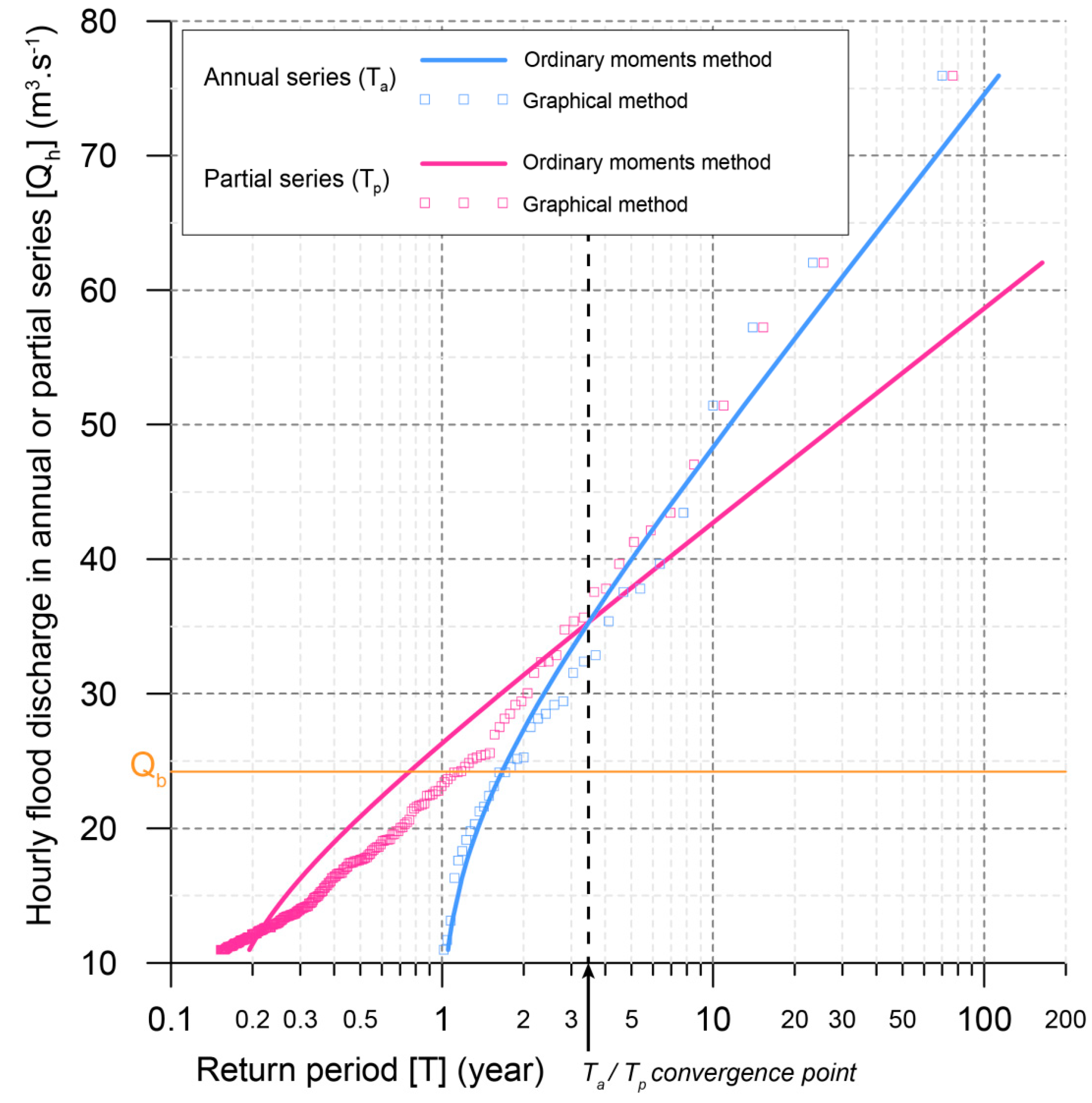
:1. Introduction
2. Materials and Methods
2.1. Study Sites
2.2. Bankfull Discharges of a Selection of Rivers in the Meuse and Scheldt Basins
2.3. Methods for Flood Return Period Estimation
2.3.1. Graphical Method and Gumbel Distribution
2.3.2. Flood Return Period Calculation in Annual Series
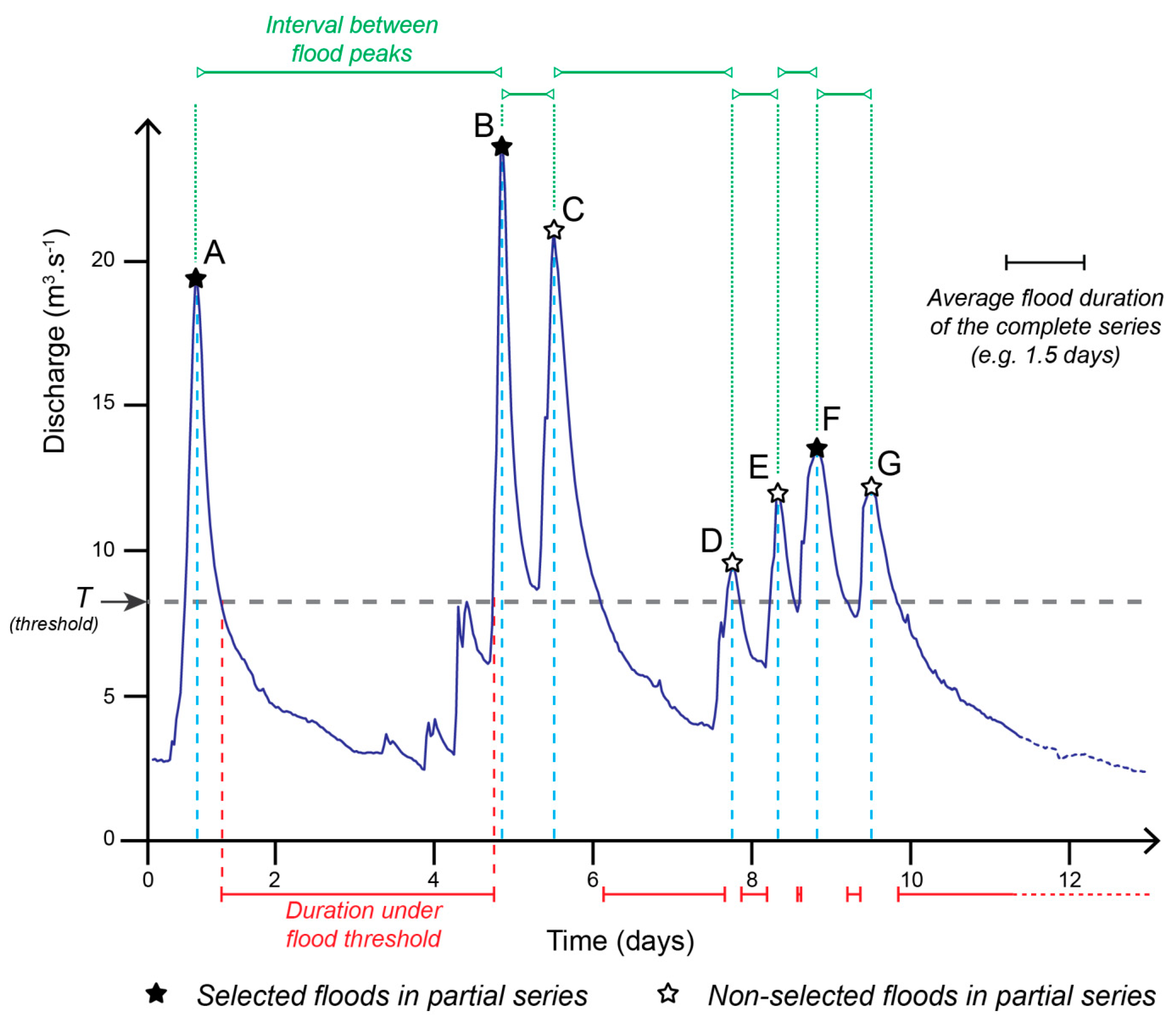
2.3.3. Flood Return Period Calculation in Partial Series
3. Results
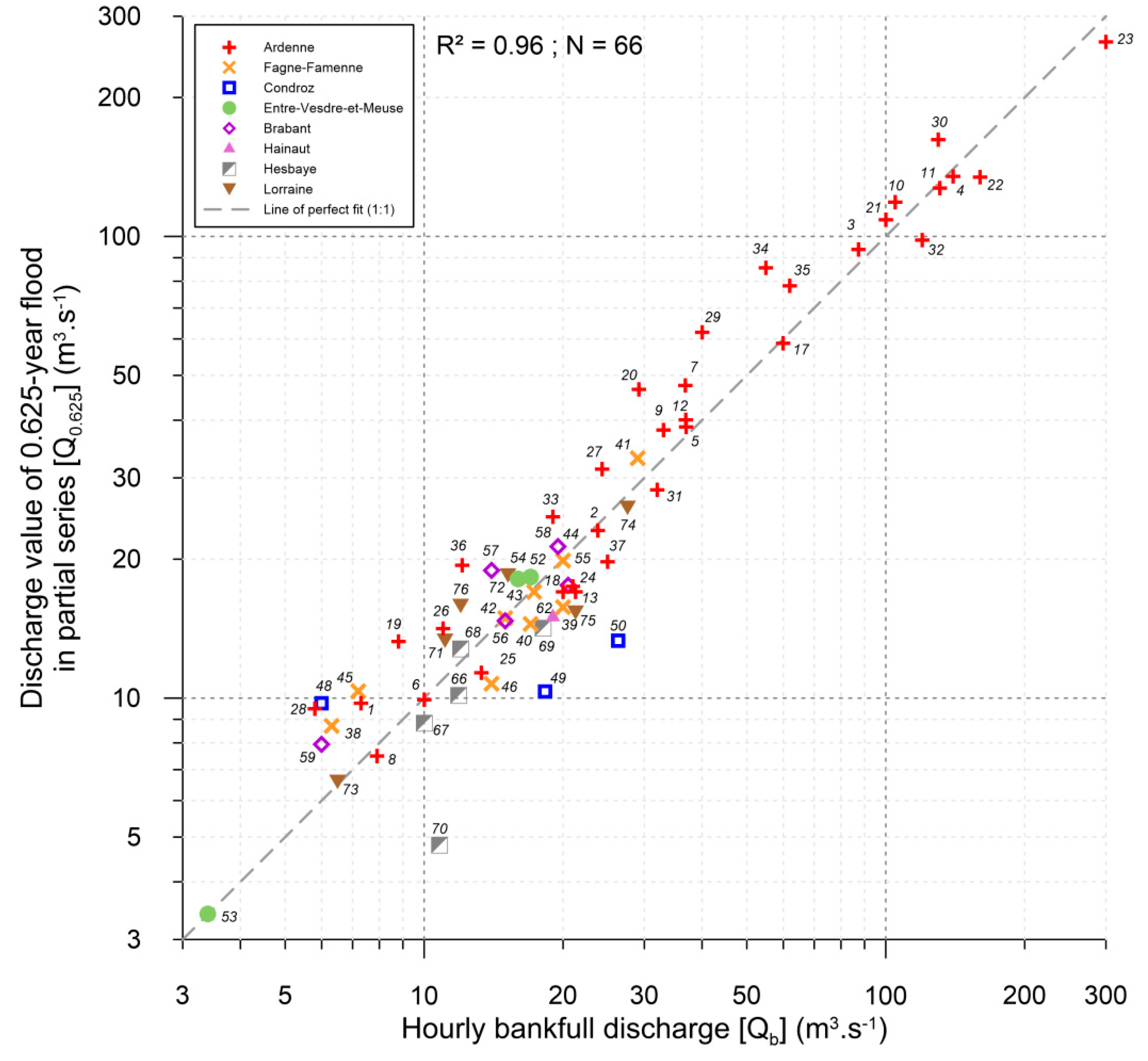
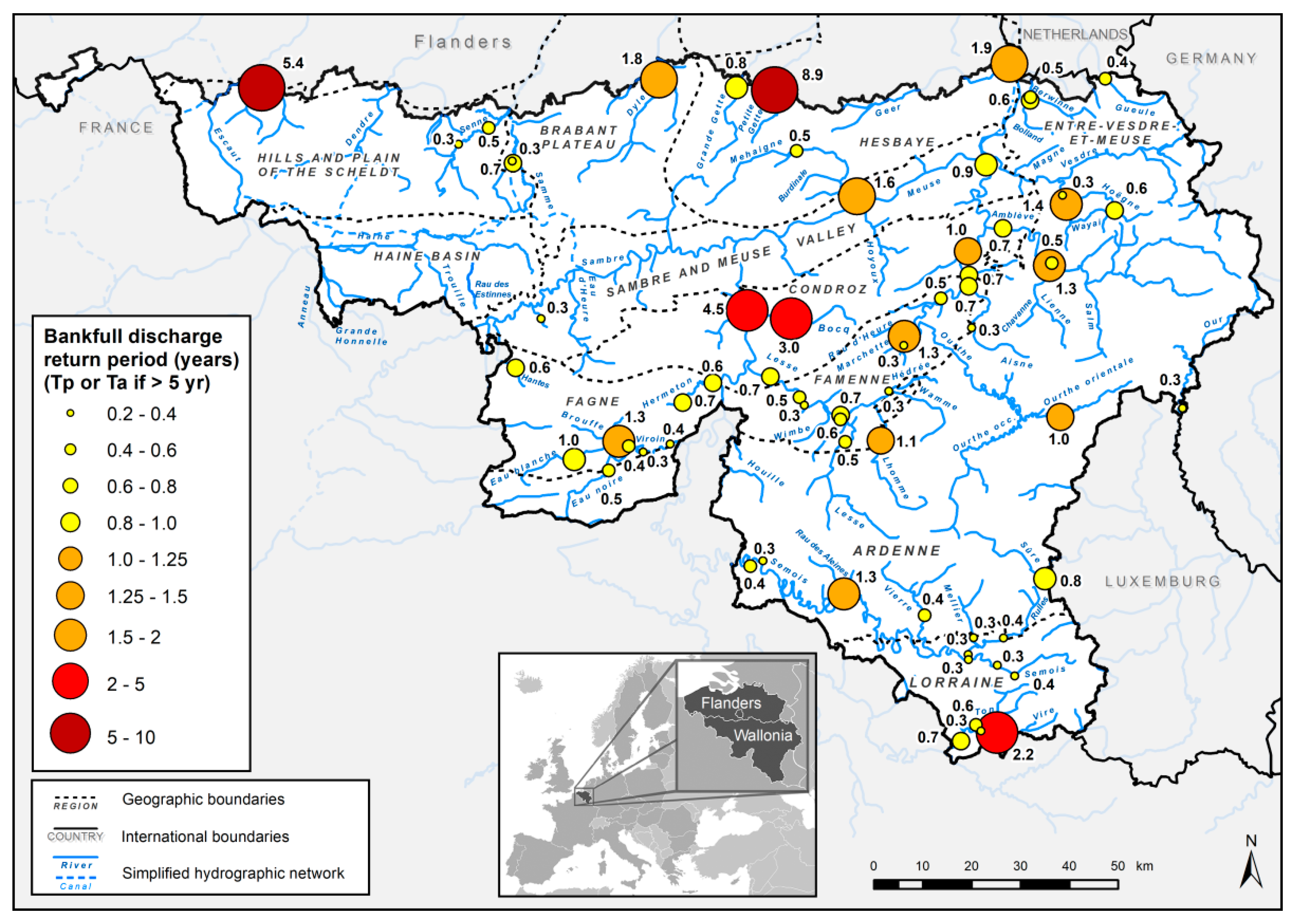
3.1. Bankfull Discharge Return Period Analysis
3.2. Discharge and Return Period of Extreme Floods
4. Discussion
5. Conclusions
Supplementary Materials
Author Contributions
Funding
Acknowledgments
Conflicts of Interest
Appendix A

| Partial Series | Annual Series | |||||||||
|---|---|---|---|---|---|---|---|---|---|---|
| ID | River | Location | Q1.5 (m3·s−1) | Q2 (m3·s−1) | Q2.33 (m3·s−1) | Q5 (m3·s−1) | Q10 (m3·s−1) | Q20 (m3·s−1) | Q50 (m3·s−1) | Q10/365 (m3·s−1) |
| 1 | Aisne | Erezée | 12.0 | 12.7 | 13.1 | 15.3 | 17.8 | 20.3 | 23.4 | 4.9 |
| 2 | Aisne | Juzaine | 30.2 | 32.4 | 33.6 | 40.0 | 48.4 | 56.4 | 66.8 | 11.0 |
| 3 | Amblève | Targnon | 117.4 | 124.7 | 128.6 | 146.8 | 171.9 | 196.1 | 227.3 | 54.0 |
| 4 | Amblève | Martinrive | 172.7 | 184.3 | 190.4 | 226.1 | 271.1 | 314.2 | 370.1 | 72.8 |
| 5 | Eau Noire | Couvin | 53.4 | 57.5 | 59.7 | 70.0 | 84.3 | 98.0 | 115.8 | 15.4 |
| 6 | Hoëgne | Belleheid | 12.3 | 13.0 | 13.4 | 16.1 | 18.8 | 21.5 | 25.0 | 2.7 |
| 7 | Hoëgne | Theux | 60.2 | 64.1 | 66.2 | 73.9 | 88.0 | 101.5 | 119.0 | 14.6 |
| 8 | Lembrée | Vieuxville | 10.1 | 10.9 | 11.3 | 13.8 | 16.7 | 19.4 | 23.0 | 2.6 |
| 9 | Lesse | Resteigne | 51.9 | 56.2 | 58.4 | 73.0 | 88.1 | 102.5 | 121.2 | 24.7 |
| 10 | Lesse | Hérock | 154.0 | 164.9 | 170.7 | 212.6 | 257.3 | 300.1 | 355.6 | 66.5 |
| 11 | Lesse | Gendron | 167.3 | 179.7 | 186.3 | 224.9 | 271.7 | 316.5 | 374.6 | 71.7 |
| 12 | Lesse | Eprave | 49.6 | 53.0 | 54.8 | 65.6 | 78.8 | 91.5 | 107.9 | 26.0 |
| 13 | Lhomme | Grupont | 21.5 | 22.8 | 23.6 | 28.7 | 34.3 | 39.6 | 46.6 | 9.1 |
| 14 | Lhomme | Forrières | 31.5 | 33.6 | 34.8 | 43.9 | 53.0 | 61.8 | 73.1 | 14.2 |
| 15 | Lhomme | Jemelle | 37.6 | 40.1 | 41.4 | 49.5 | 58.8 | 67.7 | 79.3 | 16.4 |
| 16 | Lhomme | Rochefort | 69.1 | 74.4 | 77.3 | 98.7 | 120.2 | 140.8 | 167.5 | 22.8 |
| 17 | Lhomme | Eprave | 72.2 | 76.3 | 78.5 | 92.0 | 106.2 | 119.8 | 137.4 | 29.1 |
| 18 | Lienne | Lorcé | 22.2 | 23.8 | 24.7 | 28.2 | 34.0 | 39.5 | 46.7 | 9.8 |
| 19 | Mellier | Marbehan | 18.0 | 19.5 | 20.3 | 25.1 | 30.6 | 35.9 | 42.7 | 6.9 |
| 20 | Our | Ouren | 61.3 | 65.8 | 68.2 | 79.3 | 93.6 | 107.3 | 125.1 | 29.7 |
| 21 | Ourthe | Durbuy | 138.8 | 148.0 | 152.9 | 182.9 | 218.5 | 252.6 | 296.8 | 72.4 |
| 22 | Ourthe | Tabreux | 177.9 | 191.3 | 198.3 | 242.2 | 292.5 | 340.9 | 403.4 | 91.1 |
| 23 | Ourthe | Sauheid | 341.7 | 365.5 | 378.1 | 456.6 | 546.3 | 632.4 | 743.8 | 175.6 |
| 24 | Ourthe orientale | Houffalize | 23.8 | 25.7 | 26.7 | 33.0 | 40.4 | 47.4 | 56.5 | 10.9 |
| 25 | Ruisseau des Aleines | Auby-sur-Semois | 13.7 | 14.4 | 14.7 | 16.7 | 19.1 | 21.4 | 24.3 | 8.1 |
| 26 | Rulles | Habay-la-Vieille | 18.7 | 20.1 | 20.8 | 25.0 | 29.5 | 33.8 | 39.4 | 8.5 |
| 27 | Rulles | Tintigny | 39.3 | 41.7 | 43.0 | 48.1 | 54.5 | 60.6 | 68.6 | 19.9 |
| 28 | Ry du Moulin | Vresse-sur-Semois | 12.6 | 13.6 | 14.1 | 17.8 | 21.1 | 24.2 | 28.3 | 5.6 |
| 29 | Semois | Tintigny | 81.7 | 87.8 | 91.0 | 109.7 | 132.3 | 154.0 | 182.1 | 35.5 |
| 30 | Semois | Membre Pont | 219.6 | 237.2 | 246.6 | 304.3 | 365.0 | 423.3 | 498.8 | 113.9 |
| 31 | Sûre | Martelange | 40.4 | 44.2 | 46.1 | 57.9 | 70.0 | 81.5 | 96.4 | 16.9 |
| 32 | Vesdre | Chaudfontaine | 127.0 | 135.9 | 140.6 | 164.1 | 194.1 | 222.9 | 260.2 | 40.7 |
| 33 | Vierre | Suxy | 34.7 | 37.7 | 39.3 | 49.7 | 60.0 | 69.9 | 82.7 | 17.9 |
| 34 | Viroin | Olloy-sur-Viroin | 114.4 | 123.3 | 128.0 | 149.0 | 181.1 | 211.8 | 251.7 | 35.9 |
| 35 | Viroin | Treignes | 102.0 | 109.4 | 113.4 | 138.7 | 168.0 | 196.1 | 232.5 | 36.5 |
| 36 | Wamme | Hargimont | 24.9 | 26.6 | 27.5 | 31.0 | 38.8 | 46.3 | 56.0 | 7.5 |
| 37 | Wayai | Spixhe | 25.4 | 27.2 | 28.1 | 35.0 | 41.8 | 48.4 | 56.8 | 6.3 |
| 38 | Biran | Wanlin | 11.7 | 12.7 | 13.2 | 16.7 | 20.1 | 23.3 | 27.5 | 2.2 |
| 39 | Brouffe | Mariembourg | 20.8 | 22.4 | 23.2 | 28.5 | 33.9 | 39.0 | 45.7 | 5.5 |
| 40 | Eau Blanche | Aublain | 19.1 | 20.5 | 21.2 | 26.7 | 32.0 | 37.0 | 43.5 | 7.4 |
| 41 | Eau Blanche | Nismes | 41.4 | 44.0 | 45.4 | 52.9 | 63.5 | 73.7 | 86.8 | 16.0 |
| 42 | Hantes | Beaumont | 20.6 | 22.4 | 23.3 | 30.4 | 37.6 | 44.6 | 53.5 | 4.8 |
| 43 | Hermeton | Romedenne | 22.2 | 23.8 | 24.7 | 27.7 | 33.2 | 38.5 | 45.4 | 6.0 |
| 44 | Hermeton | Hastière | 26.4 | 28.5 | 29.5 | 35.9 | 43.0 | 49.8 | 58.6 | 7.9 |
| 45 | Marchette | Marche-en-Famenne | 13.0 | 13.9 | 14.3 | 16.3 | 18.8 | 21.3 | 24.4 | 2.8 |
| 46 | Ruisseau d’Heure | Baillonville | 14.7 | 15.9 | 16.5 | 19.3 | 22.6 | 25.7 | 29.7 | 3.5 |
| 47 | Wimbe | Lavaux-Sainte-Anne | 14.7 | 15.7 | 16.2 | 19.0 | 22.1 | 25.0 | 28.8 | 5.3 |
| 48 | Biesme l’Eau | Biesme-sous-Thuin | 13.8 | 15.0 | 15.7 | 19.6 | 24.4 | 29.0 | 35.0 | 2.6 |
| 49 | Bocq | Spontin | 14.9 | 16.4 | 17.1 | 22.1 | 28.2 | 34.1 | 41.6 | 3.8 |
| 50 | Bocq | Yvoir | 19.3 | 21.2 | 22.2 | 28.2 | 36.2 | 43.9 | 53.9 | 6.5 |
| 51 | Samson | Mozet | 13.6 | 14.6 | 15.1 | 17.0 | 20.2 | 23.3 | 27.3 | 3.7 |
| 52 | Berwinne | Dalhem | 24.4 | 26.3 | 27.4 | 31.9 | 38.7 | 45.3 | 53.7 | 4.7 |
| 53 | Bolland | Dalhem | 4.4 | 4.6 | 4.8 | 5.9 | 7.2 | 8.5 | 10.2 | 1.0 |
| 54 | Gueule | Sippenaken | 23.0 | 24.5 | 25.3 | 29.1 | 33.4 | 37.5 | 42.8 | 5.1 |
| 55 | Dyle | Florival | 20.1 | 20.8 | 21.2 | 22.6 | 24.7 | 26.7 | 29.3 | 8.3 |
| 56 | Samme | Ronquières | 18.9 | 20.2 | 20.9 | 25.3 | 30.3 | 35.1 | 41.3 | 4.1 |
| 57 | Senne | Steenkerque | 24.2 | 25.9 | 26.8 | 29.9 | 35.0 | 39.9 | 46.3 | 5.1 |
| 58 | Senne | Quenast | 27.2 | 29.1 | 30.1 | 33.7 | 39.4 | 44.9 | 52.0 | 5.8 |
| 59 | Sennette | Ronquières | 10.3 | 11.0 | 11.4 | 11.2 | 13.2 | 15.1 | 17.6 | 1.9 |
| 60 | Anneau | Marchipont | 11.1 | 12.3 | 12.9 | 15.9 | 20.2 | 24.4 | 29.8 | 1.5 |
| 61 | Grande Honnelle | Baisieux | 17.2 | 18.7 | 19.4 | 23.2 | 28.7 | 34.0 | 40.9 | 3.7 |
| 62 | Rhosnes | Amougies | 17.0 | 17.6 | 17.9 | 18.7 | 21.0 | 23.2 | 26.0 | 6.7 |
| 63 | Ruisseau des Estinnes | Estinnes-au-Val | 4.4 | 4.9 | 5.1 | 6.8 | 8.8 | 10.7 | 13.3 | 0.6 |
| 64 | Trouille | Givry | 6.0 | 6.6 | 6.9 | 8.0 | 10.3 | 12.5 | 15.4 | 1.1 |
| 65 | Burdinale | Marneffe | 3.0 | 3.2 | 3.3 | 3.9 | 4.8 | 5.6 | 6.7 | 0.5 |
| 66 | Geer | Eben-Emael | 11.5 | 12.0 | 12.2 | 13.5 | 15.0 | 16.4 | 18.2 | 4.9 |
| 67 | Grande Gette | Sainte-Marie-Geest | 12.6 | 13.7 | 14.3 | 18.1 | 22.5 | 26.7 | 32.2 | 2.4 |
| 68 | Mehaigne | Ambresin | 15.5 | 16.3 | 16.7 | 17.9 | 20.7 | 23.3 | 26.8 | 5.7 |
| 69 | Mehaigne | Wanze | 17.8 | 18.9 | 19.5 | 22.5 | 26.6 | 30.6 | 35.6 | 9.0 |
| 70 | Petite Gette | Opheylissem | 6.5 | 7.0 | 7.2 | 8.9 | 11.2 | 13.4 | 16.3 | 1.6 |
| 71 | Semois | Chantemelle | 16.2 | 17.1 | 17.6 | 19.6 | 22.8 | 25.9 | 29.9 | 6.4 |
| 72 | Semois | Etalle | 21.8 | 22.8 | 23.3 | 25.5 | 29.1 | 32.5 | 36.9 | 9.9 |
| 73 | Ton | Virton | 7.6 | 8.0 | 8.1 | 8.4 | 9.4 | 10.4 | 11.6 | 3.1 |
| 74 | Ton | Harnoncourt | 34.0 | 36.6 | 37.9 | 42.6 | 52.7 | 62.4 | 75.0 | 13.3 |
| 75 | Vire | Ruette | 19.6 | 20.9 | 21.6 | 24.0 | 28.0 | 31.8 | 36.7 | 5.4 |
| 76 | Vire | Latour | 19.7 | 20.8 | 21.5 | 24.3 | 28.2 | 32.0 | 36.8 | 6.9 |
| ID | River | Location | Annual Series Equation | Partial Series Equation |
|---|---|---|---|---|
| u = a (Q − Q0) | ||||
| 1 | Aisne | Erezée | u = 0.30 (Q − 10.23) | u = 0.44 (Q − 7.55) |
| 2 | Aisne | Juzaine | u = 0.09 (Q − 23.25) | u = 0.14 (Q − 16.31) |
| 3 | Amblève | Targnon | u = 0.03 (Q − 96.49) | u = 0.04 (Q − 70.50) |
| 4 | Amblève | Martinrive | u = 0.02 (Q − 136.17) | u = 0.03 (Q − 100.69) |
| 5 | Eau Noire | Couvin | u = 0.05 (Q − 41.47) | u = 0.07 (Q − 26.01) |
| 6 | Hoëgne | Belleheid | u = 0.27 (Q − 10.47) | u = 0.41 (Q − 7.41) |
| 7 | Hoëgne | Theux | u = 0.05 (Q − 45.66) | u = 0.08 (Q − 33.75) |
| 8 | Lembrée | Vieuxville | u = 0.26 (Q − 7.95) | u = 0.38 (Q − 4.84) |
| 9 | Lesse | Resteigne | u = 0.05 (Q − 42.96) | u = 0.07 (Q − 26.32) |
| 10 | Lesse | Hérock | u = 0.02 (Q − 123.25) | u = 0.03 (Q − 83.01) |
| 11 | Lesse | Gendron | u = 0.02 (Q − 131.40) | u = 0.02 (Q − 86.35) |
| 12 | Lesse | Eprave | u = 0.06 (Q − 39.21) | u = 0.09 (Q − 28.02) |
| 13 | Lhomme | Grupont | u = 0.13 (Q − 17.44) | u = 0.22 (Q − 12.44) |
| 14 | Lhomme | Forrières | u = 0.08 (Q − 25.65) | u = 0.14 (Q − 18.43) |
| 15 | Lhomme | Jemelle | u = 0.08 (Q − 30.84) | u = 0.12 (Q − 21.56) |
| 16 | Lhomme | Rochefort | u = 0.04 (Q − 55.80) | u = 0.06 (Q − 33.60) |
| 17 | Lhomme | Eprave | u = 0.05 (Q − 63.60) | u = 0.07 (Q − 45.50) |
| 18 | Lienne | Lorcé | u = 0.13 (Q − 16.67) | u = 0.19 (Q − 12.39) |
| 19 | Mellier | Marbehan | u = 0.14 (Q − 14.12) | u = 0.21 (Q − 8.80) |
| 20 | Our | Ouren | u = 0.05 (Q − 50.72) | u = 0.07 (Q − 32.51) |
| 21 | Ourthe | Durbuy | u = 0.02 (Q − 111.73) | u = 0.03 (Q − 79.98) |
| 22 | Ourthe | Tabreux | u = 0.01 (Q − 141.54) | u = 0.02 (Q − 95.65) |
| 23 | Ourthe | Sauheid | u = 0.01 (Q − 277.26) | u = 0.01 (Q − 198.68) |
| 24 | Ourthe orientale | Houffalize | u = 0.10 (Q − 18.36) | u = 0.16 (Q − 12.09) |
| 25 | Ruisseau des Aleines | Auby-sur-Semois | u = 0.32 (Q − 12.01) | u = 0.43 (Q − 9.28) |
| 26 | Rulles | Habay-la-Vieille | u = 0.17 (Q − 16.07) | u = 0.22 (Q − 10.38) |
| 27 | Rulles | Tintigny | u = 0.12 (Q − 35.35) | u = 0.12 (Q − 23.11) |
| 28 | Ry du Moulin | Vresse-sur-Semois | u = 0.23 (Q − 11.20) | u = 0.33 (Q − 7.50) |
| 29 | Semois | Tintigny | u = 0.03 (Q − 64.46) | u = 0.05 (Q − 41.32) |
| 30 | Semois | Membre Pont | u = 0.01 (Q − 182.82) | u = 0.02 (Q − 107.00) |
| 31 | Sûre | Martelange | u = 0.06 (Q − 33.89) | u = 0.08 (Q − 16.74) |
| 32 | Vesdre | Chaudfontaine | u = 0.02 (Q − 104.10) | u = 0.03 (Q − 68.43) |
| 33 | Vierre | Suxy | u = 0.07 (Q − 29.03) | u = 0.10 (Q − 15.97) |
| 34 | Viroin | Olloy-sur-Viroin | u = 0.02 (Q − 84.88) | u = 0.03 (Q − 55.41) |
| 35 | Viroin | Treignes | u = 0.03 (Q − 80.07) | u = 0.04 (Q − 52.40) |
| 36 | Wamme | Hargimont | u = 0.10 (Q − 15.30) | u = 0.18 (Q − 13.71) |
| 37 | Wayai | Spixhe | u = 0.11 (Q − 21.47) | u = 0.17 (Q − 13.74) |
| 38 | Biran | Wanlin | u = 0.22 (Q − 9.98) | u = 0.32 (Q − 5.40) |
| 39 | Brouffe | Mariembourg | u = 0.14 (Q − 17.83) | u = 0.19 (Q − 10.30) |
| 40 | Eau Blanche | Aublain | u = 0.14 (Q − 16.27) | u = 0.22 (Q − 10.00) |
| 41 | Eau Blanche | Nismes | u = 0.07 (Q − 31.83) | u = 0.12 (Q − 24.15) |
| 42 | Hantes | Beaumont | u = 0.10 (Q − 15.99) | u = 0.17 (Q − 8.84) |
| 43 | Hermeton | Romedenne | u = 0.14 (Q − 16.63) | u = 0.19 (Q − 11.35) |
| 44 | Hermeton | Hastière | u = 0.11 (Q − 21.77) | u = 0.15 (Q − 12.75) |
| 45 | Marchette | Marche-en-Famenne | u = 0.29 (Q − 11.17) | u = 0.37 (Q − 7.45) |
| 46 | Ruisseau d’Heure | Baillonville | u = 0.23 (Q − 12.80) | u = 0.25 (Q − 6.93) |
| 47 | Wimbe | Lavaux-Sainte-Anne | u = 0.25 (Q − 12.86) | u = 0.32 (Q − 8.61) |
| 48 | Biesme l’Eau | Biesme-sous-Thuin | u = 0.16 (Q − 9.94) | u = 0.25 (Q − 5.60) |
| 49 | Bocq | Spontin | u = 0.12 (Q − 9.86) | u = 0.22 (Q − 6.20) |
| 50 | Bocq | Yvoir | u = 0.09 (Q − 12.22) | u = 0.17 (Q − 7.66) |
| 51 | Samson | Mozet | u = 0.23 (Q − 10.58) | u = 0.33 (Q − 7.45) |
| 52 | Berwinne | Dalhem | u = 0.11 (Q − 18.28) | u = 0.16 (Q − 11.60) |
| 53 | Bolland | Dalhem | u = 0.56 (Q − 3.24) | u = 1.04 (Q − 2.40) |
| 54 | Gueule | Sippenaken | u = 0.18 (Q − 20.49) | u = 0.20 (Q − 12.92) |
| 55 | Dyle | Florival | u = 0.36 (Q − 18.50) | u = 0.39 (Q − 14.84) |
| 56 | Samme | Ronquières | u = 0.15 (Q − 15.28) | u = 0.23 (Q − 10.23) |
| 57 | Senne | Steenkerque | u = 0.15 (Q − 19.74) | u = 0.18 (Q − 13.14) |
| 58 | Senne | Quenast | u = 0.13 (Q − 22.20) | u = 0.16 (Q − 14.80) |
| 59 | Sennette | Ronquières | u = 0.38 (Q − 7.29) | u = 0.42 (Q − 5.47) |
| 60 | Anneau | Marchipont | u = 0.17 (Q − 7.21) | u = 0.26 (Q − 3.39) |
| 61 | Grande Honnelle | Baisieux | u = 0.14 (Q − 12.07) | u = 0.21 (Q − 7.32) |
| 62 | Rhosnes | Amougies | u = 0.33 (Q − 14.16) | u = 0.50 (Q − 12.89) |
| 63 | Ruisseau des Estinnes | Estinnes-au-Val | u = 0.37 (Q − 2.70) | u = 0.70 (Q − 1.59) |
| 64 | Trouille | Givry | u = 0.32 (Q − 3.37) | u = 0.54 (Q − 2.27) |
| 65 | Burdinale | Marneffe | u = 0.84 (Q − 2.10) | u = 1.29 (Q − 1.39) |
| 66 | Geer | Eben-Emael | u = 0.51 (Q − 10.62) | u = 0.70 (Q − 8.61) |
| 67 | Grande Gette | Sainte-Marie-Geest | u = 0.17 (Q − 9.31) | u = 0.27 (Q − 5.77) |
| 68 | Mehaigne | Ambresin | u = 0.27 (Q − 12.34) | u = 0.37 (Q − 9.92) |
| 69 | Mehaigne | Wanze | u = 0.18 (Q − 14.37) | u = 0.28 (Q − 10.93) |
| 70 | Petite Gette | Opheylissem | u = 0.32 (Q − 4.20) | u = 0.59 (Q − 3.04) |
| 71 | Semois | Chantemelle | u = 0.23 (Q − 13.09) | u = 0.34 (Q − 10.16) |
| 72 | Semois | Etalle | u = 0.21 (Q − 18.42) | u = 0.30 (Q − 14.90) |
| 73 | Ton | Virton | u = 0.77 (Q − 6.49) | u = 0.93 (Q − 5.48) |
| 74 | Ton | Harnoncourt | u = 0.07 (Q − 22.32) | u = 0.12 (Q − 17.48) |
| 75 | Vire | Ruette | u = 0.19 (Q − 16.10) | u = 0.23 (Q − 10.82) |
| 76 | Vire | Latour | u = 0.19 (Q − 16.56) | u = 0.26 (Q − 11.74) |
Appendix B. Visual Basic Code for the Estimation of the Number of Dependent and Independent Peaks over Threshold
Appendix C. Visual Basic Code for the Calculation of the Partial Series Return Periods
References
- Dubreuil, P. Initiation à L’analyse Hydrologique; ORSTOM (Office de la Recherche Scientifique et Technique Outre-Mer): Paris, France, 1974; ISBN 2-225-40140-3. [Google Scholar]
- Bravard, J.-P.; Petit, F. Les Cours d’eau—Dynamique du Système Fluvial; Armand Colin, Collection U: Paris, France, 2000; ISBN 9782200251772. [Google Scholar]
- Assani, A.A.; Petit, F.; Mabille, G. Analyse des débits de la Warche aux barrages de Bütgenbach et de Robertville (Ardenne belge). Bull. Soc. Géogr. 1999, 36, 17–30. [Google Scholar]
- Kidson, R.; Richards, K.S. Flood frequency analysis: Assumptions and alternatives. Prog. Phys. Geogr. 2005, 29, 392–410. [Google Scholar] [CrossRef]
- Greenwood, J.A.; Landwehr, J.M.; Matalas, N.C.; Wallis, J.R. Probability weighted moments: Definition and relation to parameters of several distributions expressable in inverse form. Water Resour. Res. 1979, 15, 1049–1054. [Google Scholar] [CrossRef] [Green Version]
- Ward, A.; Moran, M. A novel approach for estimating the recurrence intervals of channel-forming discharges. Water 2016, 8, 269. [Google Scholar] [CrossRef] [Green Version]
- Petit, F.; Pauquet, A. Bankfull discharge recurrence interval in gravel-bed rivers. Earth Surf. Process. Landf. 1997, 22, 685–693. [Google Scholar] [CrossRef]
- Richards, K. Rivers, form and Process in Alluvial Channels; Methuen & Co.: London, UK, 1982; ISBN 0-416-74910-0. [Google Scholar]
- Woodyer, K.D. Bankfull frequency in rivers. J. Hydrol. 1968, 6, 114–142. [Google Scholar] [CrossRef]
- Engeland, K.; Wilson, D.; Borsányi, P.; Roald, L.; Holmqvist, E. Use of historical data in flood frequency analysis: A case study for four catchments in Norway. Hydrol. Res. 2018, 49, 466–486. [Google Scholar] [CrossRef]
- Wang, L.K.; Yang, C.T. Modern Water Resources Engineering; Humana Press: Totowa, NJ, USA, 2014; ISBN 9781627035958. [Google Scholar]
- Petit, F.; Daxhelet, C. Détermination du débit à pleins bords et de sa récurrence dans différentes rivières de moyenne et haute Belgique. Bull. Soc. Géogr. 1989, 25, 69–84. [Google Scholar]
- Louette, F. Évaluation du débit à pleins bords et de sa récurrence dans plusieurs rivières de Moyenne et Haute Belgique. Master’s Thesis, Mémoire de Licence en Sciences Géographiques, Département de Géographie, Université de Liège, Liège, Belgium, 1995. Unpublished work. [Google Scholar]
- Houbrechts, G. Utilisation des macroscories comme indicateur du transport de la charge de fond des rivières de la «Terre de Durbuy». Master’s Thesis, Mémoire de licence en Sciences géographiques, Département de Géographie, Université de Liège, Liège, Belgium, 2000. Unpublished work. [Google Scholar]
- Petit, F.; Gob, F.; Houbrechts, G.; Assani, A. Critical specific stream power in gravel-bed rivers. Geomorphology 2005, 69, 92–101. [Google Scholar] [CrossRef]
- Petit, F.; Hallot, E.; Houbrechts, G.; Mols, J. Evaluation des puissances spécifiques de rivières de moyenne et de haute Belgique. Bull. Soc. Géogr. 2005, 46, 37–50. [Google Scholar]
- Petit, F.; Hallot, E.; Houbrechts, G.; Levecq, Y.; Mols, J.; Peeters, A.; Van Campenhout, J. La typologie et les caractéristiques hydromorphologiques des cours d’eau wallons. In La Gestion Physique des Cours D’eau: Bilan D’une Décennie D’ingénierie Ecologique; Direction des Cours d’Eau Non Navigables; Direction Générale des Ressources Naturelles et de l’Environnement—Ministère de la Région Wallonne: Namur, Belgium, 2007; pp. 7–16. [Google Scholar]
- Hallot, E. Typologie hydro-géomorphologique des cours d’eau dans l’Euregio Meuse-Rhin. Ph.D. Thesis, Département de Géographie, Université de Liège, Liège, Belgium, 2010. Unpublished work. [Google Scholar]
- Peeters, A.; Houbrechts, G.; Hallot, E.; Van Campenhout, J.; Verniers, G.; Petit, F. Efficacité et résistance de techniques de protection de berges en génie végétal. Géomorphologie 2018, 24. [Google Scholar] [CrossRef]
- Guilcher, A. Précis d’Hydrologie Marine et Continentale; Masson: Paris, France, 1965. [Google Scholar]
- Réméniéras, G. L’Hydrologie de l’Ingénieur; Eyrolles: Paris, France, 1972. [Google Scholar]
- Frécaut, R. Une synthèse remarquable sur la puissance des crues de Maurice Pardé. Ann. Géogr. 1965, 74, 61–64. [Google Scholar]
- Erpicum, M.; Nouri, M.; Demoulin, A. The Climate of Belgium and Luxembourg. In Landscapes and Landforms of Belgium and Luxembourg; Demoulin, A., Ed.; Springer International Publishing: Cham, Switzerland, 2018; pp. 35–41. ISBN 9783319582399. [Google Scholar]
- Corbonnois, J.; Zumstein, J.F. Proposition de typologie des cours d’eau. Application au réseau hydrographique du Nord-Est de la France (bassin de la Moselle). Rev. Géogr. Alp. 1994, 82, 15–24. [Google Scholar] [CrossRef]
- de Béthune, P. Annexe 1. Carte géologique de la Belgique au 1/500.000. Ann. Soc. Géol. Belg. 1954. App. 1. [Google Scholar]
- Dejonghe, L. Guide de Lecture des Cartes Géologiques de Wallonie, 3rd ed.; Ministère de la Région Wallonne, Direction des Ressources Naturelles et de l’Environnment: Namur, Belgium, 2007. [Google Scholar]
- Williams, G.P. Bank-full discharge of rivers. Water Resour. Res. 1978, 14, 1141–1154. [Google Scholar] [CrossRef]
- Navratil, O.; Albert, M.-B.; Hérouin, E.; Gresillon, J.-M. Determination of bankfull discharge magnitude and frequency: Comparison of methods on 16 gravel-bed river reaches. Earth Surf. Process. Landf. 2006, 31, 1345–1363. [Google Scholar] [CrossRef]
- Gob, F.; Bilodeau, C.; Thommeret, N.; Belliard, J.; Albert, M.-B.; Tamisier, V.; Baudoin, J.-M.; Kreutzenberger, K. Un outil de caractérisation hydromorphologique des cours d’eau pour l’application de la DCE en France (CARHYCE) A tool for the characterisation of the hydromorphology of rivers in line with the application of the European Water Framework Directive in France. Géomorphologie 2014, 20, 57–72. [Google Scholar]
- Morel, M.; Tamisier, V.; Pella, H.; Booker, D.J.; Navratil, O.; Piégay, H.; Gob, F.; Lamouroux, N. Revisiting the drivers of at-a-station hydraulic geometry in stream reaches. Geomorphology 2019, 328, 44–56. [Google Scholar] [CrossRef]
- Navratil, O.; Albert, M.B.; Breil, P. Test of three methods to detect the overbank flow from water level time-series analysis. Hydrol. Process. 2010, 24, 2452–2464. [Google Scholar] [CrossRef]
- Gomez, B.; Coleman, S.E.; Sy, V.W.K.; Peacock, D.H.; Kent, M. Channel change, bankfull and effective discharges on a vertically accreting, meandering, gravel-bed river. Earth Surf. Process. Landf. 2007, 32, 770–785. [Google Scholar] [CrossRef]
- Ahilan, S.; O’Sullivan, J.J.; Bruen, M.; Brauders, N.; Healy, D. Bankfull discharge and recurrence intervals in Irish rivers. Proc. Inst. Civ. Eng. Water Manag. 2013, 166, 381–393. [Google Scholar] [CrossRef] [Green Version]
- Lawlor, S.M. Determination of Channel-Morphology Characteristics, Bankfull Discharge, and Various Design-Peak Discharges in Western Montana; US Geological Survey: Reston, VA, USA, 2004. [Google Scholar]
- Agouridis, C. Bankfull Frequency in Rivers. In Handbook of Engineering Hydrology; CRC Press: Boca Raton, FL, USA, 2014; pp. 35–51. ISBN 9781466552470. [Google Scholar]
- Castro, J.M.; Jackson, P.L. Bankfull discharge recurrence intervals and regional hydraulic geometry relationships: Patterns in the Pacific Northwest, USA. J. Am. Water Resour. Assoc. 2001, 37, 1249–1262. [Google Scholar] [CrossRef]
- Dury, G.H. Magnitude–frequency analysis and channel morphology. In Fluvial Geomorphology; Morisawa, M., Ed.; State University of N.Y. at Binghamton: Binghamton, NY, USA, 1973; pp. 91–121. [Google Scholar]
- Tricart, J. Précis de Géomorphologie. 2. Géomorphologie, Dynamique Générale; Société d’Edition d’Enseignement Supérieur: Paris, France, 1977. [Google Scholar]
- Amoros, C.; Petts, G.E. Hydrosystèmes Fluviaux; Amoros, C., Petts, G.E., Eds.; Masson, Coll. Écologie: Paris, France, 1993. [Google Scholar]
- Edwards, P.J.; Watson, E.A.; Wood, F. Toward a Better Understanding of Recurrence Intervals, Bankfull, and Their Importance. J. Contemp. Water Res. Educ. 2019, 166, 35–45. [Google Scholar] [CrossRef] [Green Version]
- Wilkerson, G.V. Improved bankfull discharge prediction using 2-year recurrence-period discharge. JAWRA J. Am. Water Resour. Assoc. 2008, 44, 243–257. [Google Scholar] [CrossRef]
- Houbrechts, G. Utilisation des macroscories et des microscories en dynamique fluviale: Application aux rivières du massif ardennais (Belgique). Ph.D. Thesis, Département de Géographie, Université de Liège, Liège, Belgium, 2005. Unpublished work. [Google Scholar]
- Deroanne, C. Dynamique fluviale de la Hoëgne. Évaluation longitudinale des caractéristiques sédimentologiques du lit et des paramètres de mobilisation de la charge de fond. Master’s Thesis, Mémoire de Licence en Sciences Géographiques, Université de Liège, Liège, Belgium, 1995. Unpublished work. [Google Scholar]
- Franchimont, C. Dynamique fluviale de la Lesse: Fréquence des inondations, morphométrie des méandres et sédimentologie du lit. Master’s Thesis, Mémoire de Licence en Sciences Géographiques, Université de Liège, Liège, Belgium, 1993. Unpublished work. [Google Scholar]
- Petit, F.; Houbrechts, G.; Peeters, A.; Hallot, E.; Van Campenhout, J.; Denis, A.-C. Dimensionless critical shear stress in gravel-bed rivers. Geomorphology 2015, 250, 308–320. [Google Scholar] [CrossRef]
- Pauquet, A.; Petit, F. Evolution de la fréquence des inondations de l’Ourthe inférieure. Bull. Soc. Belg. Géogr. 1993, 2, 361–375. [Google Scholar]
- Jacquemin, I. Dynamique fluviale d’une rivière à blocs: Le Ruisseau de Ruaumoulin (Affluent de la Semois ardennaise). Master’s Thesis, Mémoire de Licence en Sciences Géographiques, Université de Liège, Liège, Belgium, 2008. Unpublished work. [Google Scholar]
- Gob, F.; Houbrechts, G.; Hiver, J.M.; Petit, F. River dredging, channel dynamics and bedload transport in an incised meandering river (the River Semois, Belgium). River Res. Appl. 2005, 21, 791–804. [Google Scholar] [CrossRef]
- Vanderheyden, V. Dynamique fluviale du Viroin. Contribution à la détermination des zones inondables du bassin, évolution des inondations, morphométrie et transport de la charge de fond. Master’s Thesis, Mémoire de Licence en Sciences Géographiques, Université de Liège, Liège, Belgium, 2003. Unpublished work. [Google Scholar]
- Peeters, A.; Hallot, E.; Houbrechts, G.; Verniers, G.; de le Court, B.; Petit, F. Suivi géomorphologique de la restauration de la continuité longitudinale du Bocq. In La Restauration Hydromorphologique des Cours d’Eau: Premiers Enseignements du Projet LIFE WALPHY; SPW: Namur, Belgium, 2013. [Google Scholar]
- Houbrechts, G.; Levecq, Y.; Peeters, A.; Hallot, E.; Van Campenhout, J.; Denis, A.-C.; Petit, F. Evaluation of long-term bedload virtual velocity in gravel-bed rivers (Ardenne, Belgium). Geomorphology 2015, 251, 6–19. [Google Scholar] [CrossRef]
- Mols, J. Dynamique fluviale en réponse aux changements d’affectation du sol des bassins versants de l’Euregio Meuse-Rhin. Master’s Thesis, Mémoire de Licence en Sciences Géographiques, Université de Liège, Liège, Belgium, 2004. Unpublished work. [Google Scholar]
- Denis, A.-C.; Van Campenhout, J.; Hallot, E.; Houbrechts, G. Développement d’outils d’évaluation des variations qualitatives et quantitatives des gisements de sédiments dans les cours d’eau navigables et non navigables. Identification des interactions entre les deux gisements via les phénomènes de transport. Projet-GISSED; ISSeP: Liège, Belgium, 2014. [Google Scholar]
- Mabille, G.; Petit, F. Influence des aménagements du cours d’une rivière de Moyenne Belgique et de son bassin hydrographique, sur le comportement hydrologique de la rivière. In Crues et Inondations; Humbert, J., Ed.; CEREG/ULP: Strasbourg, France, 1987; pp. 279–293. [Google Scholar]
- Perpinien, G. Dynamique fluviale de la Mehaigne. Morphométrie, transports en solution et en suspension, mobilisation de la charge de fond. Master’s Thesis, Mémoire de Licence en Sciences Géographiques, Université de Liège, Liège, Belgium, 1998. Unpublished work. [Google Scholar]
- Meylan, P.; Favre, A.-C.; Musy, A. Predictive Hydrology—A Frequency Analysis Approach; CRC Press: Boca Raton, FL, USA, 2011; ISBN 9781439807132. [Google Scholar]
- Hazen, A. Flood Flows; John Wiley & Sons: New York, NY, USA, 1930. [Google Scholar]
- Brunet-Moret, Y. Statistiques de rangs. Cah. Orstom. Série Hydrol. 1973, 10, 133–151. [Google Scholar]
- Fisher, R.A.; Tippett, L.H.C. Limiting forms of the frequency distribution of the largest or smallest member of a sample. Proc. Camb. Philos. Soc. 1928, 24, 180–190. [Google Scholar] [CrossRef]
- Gumbel, E.J. Floods estimated by probability method. Eng. News Rec. 1945, 134, 833–837. [Google Scholar]
- Gumbel, E.J. Statistics of Extremes, 2nd ed.; Columbia University Press: New York, NY, USA, 1960. [Google Scholar]
- Meylan, P.; Favre, A.C.; Musy, A. Hydrologie Fréquentielle: Une Science Prédictive; Presses Polytechniques et Universitaires Romandes, Science & Ingénierie de l’Environnement: Lausanne, Switzerland, 2008; ISBN 9782880747978. [Google Scholar]
- Keast, D.; Ellison, J. Magnitude frequency analysis of small floods using the annual and partial series. Water 2013, 5, 1816–1829. [Google Scholar] [CrossRef] [Green Version]
- Bernier, J. Sur l’application des diverses lois limites des valeurs extrêmes au problème des débits de crues. Rev. Stat. Appl. 1957, 5, 91–101. [Google Scholar]
- Bernier, J.; Veron, R. Sur quelques difficultés rencontrées dans l’estimation d’un débit de crue de probabilité donnée. Rev. Stat. Appl. 1964, 12, 25–48. [Google Scholar]
- Karim, F.; Hasan, M.; Marvanek, S. Evaluating Annual Maximum and Partial Duration Series for Estimating Frequency of Small Magnitude Floods. Water 2017, 9, 481. [Google Scholar] [CrossRef] [Green Version]
- Langbein, W.B. Annual floods and the partial-duration flood series. Trans. Am. Geophys. Union 1949, 30, 120–130. [Google Scholar] [CrossRef]
- Lang, M.; Ouarda, T.B.M.J.; Bobée, B. Towards operational guidelines for over-threshold modeling. J. Hydrol. 1999, 225, 103–117. [Google Scholar] [CrossRef]
- Rosbjerg, D.; Madsen, H. On the Choice of Threshold Level in Partial Durations Series; Østrem, G., Ed.; NHP Rep.: Alta, Norway, 1992. [Google Scholar]
- Dunne, T.; Leopold, L.B. Water in Environmental Planning; Freeman, W.H., Ed.; Freeman & Co.: San Francisco, CA, USA, 1978. [Google Scholar]
- Ashkar, F.; Rousselle, J. Some remarks on the truncation used in partial flood series models. Water Resour. Res. 1983, 19, 477–480. [Google Scholar] [CrossRef]
- Konecny, F.; Nachtnebel, H.P. Extreme value processes and the evaluation of risk in flood analysis. Appl. Math. Model. 1985, 9, 11–15. [Google Scholar] [CrossRef]
- Miquel, J. Guide Pratique d’Estimation des Probabilités de Crue; Eyrolles: Paris, France, 1984. [Google Scholar]
- Guidelines for Determining Flood Flow Frequency. Bulletin no. 17B of the Hydrology Subcommittee; U.S. Department of the Interior. Geological Survey. Office of Water Data Coordination: Washington, DC, USA, 1976. [Google Scholar]
- Brodie, I.M.; Khan, S. A direct analysis of flood interval probability using approximately 100-year streamflow datasets. Hydrol. Sci. J. 2016, 61, 2213–2225. [Google Scholar] [CrossRef] [Green Version]
- Cunnane, C. A particular comparison of annual maxima and partial duration series methods of flood frequency prediction. J. Hydrol. 1973, 18, 257–271. [Google Scholar] [CrossRef]
- Irvine, K.N.; Waylen, P.R. Partial Series Analysis of High Flows in Canadian Rivers. Can. Water Resour. J. 1986, 11, 83–91. [Google Scholar] [CrossRef] [Green Version]
- Adamowski, K. Regional analysis of annual maximum and partial duration flood data by nonparametric and L-moment methods. J. Hydrol. 2000, 229, 219–231. [Google Scholar] [CrossRef]
- Rosbjerg, D.; Madsen, H.; Rasmussen, P.F. Prediction in partial duration series with generalized pareto-distributed exceedances. Water Resour. Res. 1992, 28, 3001–3010. [Google Scholar] [CrossRef]
- Dalrymple, T. Flood-Frequency Analysis (Water-Supply Paper, 1543A); US Geological Survey: Reston, VA, USA, 1960. [Google Scholar]
- Claps, P.; Laio, F. Can continuous streamflow data support flood frequency analysis? An alternative to the partial duration series approach. Water Resour. Res. 2003, 39, 1–11. [Google Scholar] [CrossRef] [Green Version]
- Klein, T. Comparaison des sécheresses estivales de 1976 et 2003 en Europe occidentale à l’aide d’indices climatiques. Bull. Soc. Géogr. 2009, 53, 75–86. [Google Scholar]
- Van Campenhout, J.; Denis, A.-C.; Hallot, E.; Houbrechts, G.; Levecq, Y.; Peeters, A.; Petit, F. Flux des sédiments en suspension dans les rivières du bassin de la Meuse: Proposition d’une typologie régionale basée sur la dénudation spécifique des bassins versants. Bull. Soc. Géogr. 2013, 61, 15–36. [Google Scholar]
- Beckers, A. Facteurs de propagation des knickpoints dans un réseau hydrographique—Modélisation dans le bassin de l’. Ourthe. Thesis, Mémoire de Licence en Sciences Géographiques, Université de Liège, Liège, Belgium, 2010. Unpublished work. [Google Scholar]
- Gailliez, S. Estimation des Débits d’Etiage Pour des Sites Non Jaugés. Application en Région Wallonne. Ph.D. Thesis, Université de Liège—Gembloux Agro-Bio Tech, Liège, Belgium, 2013. [Google Scholar]
- Herschy, R.W. The world’s maximum observed floods. Flow Meas. Instrum. 2002, 13, 231–235. [Google Scholar] [CrossRef]
- Costa, J.E. A comparison of the largest rainfall-runoff floods in the United States with those of the People’s Republic of China and the world. J. Hydrol. 1987, 96, 101–115. [Google Scholar] [CrossRef]
- Van Campenhout, J.; Hallot, E.; Houbrechts, G.; Peeters, A.; Levecq, Y.; Gérard, P.; Petit, F. Flash floods and muddy floods in Wallonia: Recent temporal trends, spatial distribution and reconstruction of the hydrosedimentological fluxes using flood marks and sediment deposits. Belgeo 2015, 1, 1–22. [Google Scholar] [CrossRef] [Green Version]
- De Schryver, R.; Lignon, Y.; Brixko, J. Le démergement de la région liégeoise. In Proceedings of the Après-Mines 2003, Nancy, France, 5–7 February 2003; p. 11. [Google Scholar]
- Drogue, G.; Fournier, M.; Bauwens, A.; Commeaux, F.; De Keizer, O.; François, D.; Guilmin, E.; Degré, A.; Detrembleur, S.; Dewals, B.; et al. Analysis of Climate Change, High-Flows and Low-Flows Scenarios on the Meuse Basin; EPAMA - EPTB Meuse: Charleville-Mézières, France, 2010. [Google Scholar]
- Pardé, M. Fleuves et Rivières; Colin, A., Ed.; Colin: Paris, France, 1963. [Google Scholar]
- Cosandey, C. Les Eaux Courantes; Editions, B., Ed.; Belin: Paris, France, 2003. [Google Scholar]
- Douvinet, J. Les bassins versants sensibles aux ”crues rapides” dans le Bassin Parisien—Analyse de la structure et de la dynamique de systèmes spatiaux complexes. Ph.D. Thesis, Université de Caen, Caen, France, 2008. [Google Scholar]
- Pissart, A. Les inondations dans la région de Verviers-Eupen. Etude préalable à un aménagement du territoire. Bull. Cebedeau 1961, 123, 62–75. [Google Scholar]
- Petit, F. Régime hydrologique et dynamique fluviale des rivières ardennaises. In L’Ardenne: Essai de Géographie Physique; Demoulin, A., Ed.; Université de Liège: Liège, Belgium, 1995; pp. 194–223. [Google Scholar]
- Gob, F.; Petit, F.; Bravard, J.-P.; Ozer, A.; Gob, A. Lichenometric application to historical and subrecent dynamics and sediment transport of a Corsican stream (Figarella River—France). Quat. Sci. Rev. 2003, 22, 2111–2124. [Google Scholar] [CrossRef] [Green Version]
- Francou, J.; Rodier, J.A. Essai de classification des crues maximales observées dans le monde. Cah. Orstom Série Hydrol. 1967, 4, 19–46. [Google Scholar]
- Ferro, V.; Porto, P. Identifying a dominant discharge for natural rivers in southern Italy. Geomorphology 2012, 139–140, 313–321. [Google Scholar] [CrossRef]
- Andrews, E.D. Effective and bankfull discharges of streams in the Yampa River basin, Colorado and Wyoming. J. Hydrol. 1980, 46, 311–330. [Google Scholar] [CrossRef]
- Erskine, W.D. Frequency of Bankfull Discharge on South and Eastern Creeks. In Handbook of Engineering Hydrology; Eslamian, S., Ed.; CRC Press: Boca Raton, FL, USA, 2014. [Google Scholar]
- Elabdellaoui, J.E. Fréquence et prédétermination des crues (Essai d’une typologie régionale appliquée à la Moyenne et à la Haute Belgique). Master’s Thesis, Mémoire de Maitrise en Géologie des Terrains Superficiels, Université de Liège, Liège, Belgium, 1993. Unpublished work. [Google Scholar]
- Shuster, W.D.; Bonta, J.; Thurston, H.; Warnemuende, E.; Smith, D.R. Impacts of impervious surface on watershed hydrology: A review. Urban Water J. 2005, 2, 263–275. [Google Scholar] [CrossRef]
- Markus, M.; Cai, X.; Sriver, R. Extreme floods and droughts under future climate scenarios. Water 2019, 11, 1720. [Google Scholar] [CrossRef] [Green Version]
- Vandiepenbeeck, M. Aperçu des caractéristiques climatiques constatées à Bruxelles-Uccle durant la période trentenaire 1988–2007. Bull. Soc. Géogr. 2008, 51, 151–162. [Google Scholar]
- Rigal, A.; Azaïs, J.M.; Ribes, A. Estimating daily climatological normals in a changing climate. Clim. Dyn. 2019, 53, 275–286. [Google Scholar] [CrossRef] [Green Version]


| ID | River | Location | A (km2) | Station Code | Station Start Date | Ny | Qb (m3·s−1) | Specific Qb (m3·s−1·km−2) | Sources of Qb Observation |
|---|---|---|---|---|---|---|---|---|---|
| ARDENNE Region | |||||||||
| 1 | Aisne | Erezée | 67.4 | L6690 | 1998–12 | 20 | 7.3 | 0.108 | Houbrechts (2000) [14] |
| 2 | Aisne | Juzaine | 183 | L5491 | 1975–03 | 34 | 23.8 | 0.130 | Houbrechts (2000) [14] |
| 3 | Amblève | Targnon | 802.9 | S6671 | 1968–06 | 20 | 87.3 | 0.109 | New observation |
| 4 | Amblève | Martinrive | 1062 | S6621 | 1968–10 | 45 | 140 | 0.132 | Houbrechts (2005) [42] |
| 5 | Eau Noire | Couvin | 176 | S9071 | 1968–03 | 33 | 36.9 | 0.210 | New observation (2008) |
| 6 | Hoëgne | Belleheid | 20 | S6526 | 1993–06 | 25 | 10 | 0.500 | New observation (2019) |
| 7 | Hoëgne | Theux | 189 | L5860 | 1979–02 | 36 | 36.8 | 0.195 | Deroanne (1995) [43] |
| 8 | Lembrée | Vieuxville | 51 | L6300 | 1991–09 | 26 | 7.9 | 0.155 | Houbrechts (2005) [42] |
| 9 | Lesse | Resteigne | 345 | L5021 | 1992–06 | 46 | 33 | 0.096 | Franchimont (1993) [44] |
| 10 | Lesse | Hérock | 1156 | L6610 | 1996–05 | 23 | 105 | 0.091 | Bioengineering techniques report (2016) |
| 11 | Lesse | Gendron | 1286 | S8221 | 1968–01 | 51 | 131 | 0.102 | Bioengineering techniques report (2016) |
| 12 | Lesse | Eprave | 419 | L5080 | 1969–01 | 41 | 37 | 0.088 | Petit et al. (2015) [45] |
| 13 | Lhomme | Grupont | 179.9 | L6360 | 1991–10 | 22 | 20 | 0.111 | Franchimont (1993) [44] |
| 14 | Lhomme | Forrières | 247 | L6310 | 1991–10 | 24 | 24.51 | 0.099 | Computed Q0.625 |
| 15 | Lhomme | Jemelle | 276 | S8527 | 1969–01 | 50 | 29.71 | 0.108 | Computed Q0.625 |
| 16 | Lhomme | Rochefort | 424.9 | L6650 | 1996–07 | 22 | 51.81 | 0.122 | Computed Q0.625 |
| 17 | Lhomme | Eprave | 478 | L6360 | 1992–07 | 24 | 60 | 0.126 | Petit et al. (2015) [45] |
| 18 | Lienne | Lorcé | 147 | L6240 | 1992–09 | 25 | 21.3 | 0.145 | Houbrechts (2005) [42] and new authors observation (2008) |
| 19 | Mellier | Marbehan | 62 | L5500 | 1974–06 | 39 | 8.8 | 0.142 | New observation (2008) |
| 20 | Our | Ouren | 386 | L6330 | 1991–09 | 26 | 29.2 | 0.076 | New observation (2005) |
| 21 | Ourthe | Durbuy | 1285 | S5953 | 1994–12 | 24 | 100 | 0.078 | New observation |
| 22 | Ourthe | Tabreux | 1597 | S5921 | 1970–12 | 48 | 160 | 0.100 | Petit & Daxhelet (1989) [12] |
| 23 | Ourthe | Sauheid | 2910 | S5826 | 1974–01 | 45 | 300 | 0.103 | Pauquet & Petit (1993) [46] |
| 24 | Ourthe orientale | Houffalize | 179 | L5930 | 1979–02 | 37 | 21 | 0.117 | Petit et al. (2015) [45] |
| 25 | Ruisseau des Aleines | Auby-sur-Semois | 88.4 | L6990 | 2003–09 | 15 | 13.3 | 0.150 | New observation (2018) |
| 26 | Rulles | Habay-la-Vieille | 96 | L5970 | 1981–11 | 33 | 11 | 0.115 | Petit and Pauquet (1997) [7] |
| 27 | Rulles | Tintigny | 219 | L5220 | 1971–02 | 39 | 24.3 | 0.111 | New observation (2008) |
| 28 | Ry du Moulin | Vresse-sur-Semois | 61.8 | L7000 | 2003–09 | 15 | 5.8 | 0.094 | Jacquemin [47] |
| 29 | Semois | Tintigny | 380.9 | S9561 | 1974–01 | 45 | 40 | 0.105 | New observation (2008) |
| 30 | Semois | Membre Pont | 1235 | S9434 | 1968–01 | 51 | 130 | 0.105 | Petit & Pauquet (1997) [7], Gob et al. (2005) [48] |
| 31 | Sûre | Martelange | 209 | L5610 | 1975–03 | 40 | 32 | 0.153 | Peeters et al. (2018) [19] |
| 32 | Vesdre | Chaudfontaine | 683 | S6228 | 1975–06 | 43 | 120 | 0.176 | Petit & Daxhelet (1989) [12] |
| 33 | Vierre | Suxy | 219.8 | L7140 | 2003–12 | 15 | 19 | 0.086 | New observation (2008) |
| 34 | Viroin | Olloy-sur-Viroin | 491 | L6380 | 1992–01 | 26 | 55 | 0.112 | New observation (2011) |
| 35 | Viroin | Treignes | 548 | S9021 | 1968–01 | 45 | 62 | 0.113 | New observation (2009) |
| 36 | Wamme | Hargimont | 80 | L6370/L7640 | 2011–06 | 13 | 12.1 | 0.151 | New observation (2008) |
| 37 | Wayai | Spixhe | 93.8 | L6790 | 2002–03 | 17 | 25 | 0.267 | New estimate |
| FAGNE–FAMENNE Region | |||||||||
| 38 | Biran | Wanlin | 51.9 | L7190 | 2004–09 | 14 | 6.3 | 0.121 | New observation (2008) |
| 39 | Brouffe | Mariembourg | 80 | S9111 | 1981–01 | 38 | 20 | 0.250 | New observation (2009) |
| 40 | Eau Blanche | Aublain | 106.2 | L6530 | 1994–03 | 24 | 17 | 0.160 | New observation (2011) |
| 41 | Eau Blanche | Nismes | 254 | S9081 | 1968–01 | 50 | 29 | 0.114 | Vanderheyden [49] and new observation (2013) |
| 42 | Hantes | Beaumont | 92.4 | L6880 | 2003–03 | 15 | 15 | 0.162 | New observation |
| 43 | Hermeton | Romedenne | 115 | L5060 | 1969–02 | 48 | 17.3 | 0.150 | New observation (2008) |
| 44 | Hermeton | Hastière | 166 | S8622 | 1967–09 | 50 | 20 | 0.120 | New observation (2008) |
| 45 | Marchette | Marche-en-Famenne | 48.9 | L7120 | 2003–12 | 15 | 7.2 | 0.147 | Petit & Daxhelet (1989) [12] |
| 46 | Ruisseau d’Heure | Baillonville | 68 | L6050 | 1984–06 | 29 | 14 | 0.206 | Louette (1995) [13] |
| 47 | Wimbe | Lavaux-Sainte-Anne | 93 | L6270 | 1991–08 | 26 | 11.7 1 | 0.125 | Computed Q0.625 |
| CONDROZ Region | |||||||||
| 48 | Biesme l’Eau | Biesme-sous-Thuin | 79.8 | L7180 | 2004–09 | 14 | 6 | 0.075 | New observation |
| 49 | Bocq | Spontin 2 | 163.6 | L7320 | 2006–04 | 40 | 18.3 | 0.112 | Petit et al. (2015) [45] |
| 50 | Bocq | Yvoir | 230 | L5800 | 1979–02 | 39 | 26.3 | 0.114 | Peeters et al. (2013) [50] |
| 51 | Samson | Mozet | 108.2 | L5980 | 1982–10 | 26 | 10.6 1 | 0.098 | Computed Q0.625 |
| ENTRE–VESDRE–ET–MEUSE Region | |||||||||
| 52 | Berwinne | Dalhem | 118 | L6390 | 1991–12 | 24 | 17 | 0.144 | Houbrechts et al. (2015) [51] |
| 53 | Bolland | Dalhem | 29.3 | L6770 | 2001–12 | 17 | 3.4 | 0.116 | New observation |
| 54 | Gueule | Sippenaken | 121 | L6660 | 1996–06 | 22 | 16 | 0.132 | Mols (2004) [52] |
| BRABANT Region | |||||||||
| 55 | Dyle | Florival | 430 | L6160 | 1992–07 | 23 | 20.5 | 0.048 | New observation (2011) |
| 56 | Samme | Ronquières | 135 | S2371 | 1971–08 | 30 | 15 | 0.111 | Denis et al. (2014) [53] |
| 57 | Senne | Steenkerque | 116 | L5660 | 1996–06 | 40 | 14 | 0.121 | SPW data |
| 58 | Senne | Quenast | 169 | 1977–03 | 40 | 19.5 | 0.115 | New observation (2011) | |
| 59 | Sennette | Ronquières | 70 | L5670 | 1977–07 | 28 | 6 | 0.086 | SPW data |
| HAINAUT Region | |||||||||
| 60 | Anneau | Marchipont | 78.2 | L6870 | 2003–03 | 15 | 7.3 1 | 0.094 | Computed Q0.625 |
| 61 | Grande Honnelle | Baisieux | 121 | L5170 | 1971–01 | 40 | 12.4 1 | 0.103 | Computed Q0.625 |
| 62 | Rhosnes | Amougies | 165 | L5412 | 1972–02 | 38 | 19 | 0.115 | SPW data |
| 63 | Ruisseau des Estinnes | Estinnes-au-Val | 28.7 | L7080 | 2003–11 | 15 | 3.0 1 | 0.105 | Computed Q0.625 |
| 64 | Trouille | Givry | 55.7 | L6710 | 2000–05 | 19 | 4.2 1 | 0.075 | Computed Q0.625 |
| HESBAYE Region | |||||||||
| 65 | Burdinale | Marneffe | 26.8 | L6461 | 2008–09 | 10 | 2.2 1 | 0.082 | Computed Q0.625 |
| 66 | Geer | Eben-Emael | 452.3 | L6340 | 1991–08 | 23 | 11.9 | 0.026 | Mabille & Petit (1987) [54] |
| 67 | Grande Gette | Sainte-Marie-Geest | 135 | L5720 | 1978–01 | 41 | 10 | 0.074 | New observation (2011) |
| 68 | Mehaigne | Ambresin | 194.7 | L6470 | 1991–12 | 25 | 12 | 0.062 | Peeters et al. (2018) [19] |
| 69 | Mehaigne | Wanze | 352 | L5820 | 1978–12 | 39 | 18.1 | 0.051 | Perpinien (1998) [55] at Moha |
| 70 | Petite Gette | Opheylissem | 134 | L6280 | 1991–08 | 25 | 4.8 1 | 0.081 | Computed Q0.625 |
| LORRAINE Region | |||||||||
| 71 | Semois | Chantemelle | 89 | L5880 | 1979–01 | 40 | 11.1 | 0.125 | New observation (2001) |
| 72 | Semois | Etalle | 123.9 | L6180 | 1992–09 | 25 | 15.2 | 0.123 | New observation (2008) |
| 73 | Ton | Virton | 89 | L6440 | 1991–08 | 25 | 6.5 | 0.073 | New observation (2007) |
| 74 | Ton | Harnoncourt | 293 | L5520 | 1974–03 | 44 | 27.6 | 0.094 | New observation (2008) |
| 75 | Vire | Ruette | 104 | L5600 | 1975–07 | 39 | 21.3 | 0.205 | SPW data and new estimate |
| 76 | Vire | Latour | 125 | L6030 | 1983–10 | 34 | 12 | 0.096 | New observation (2008) |
| Threshold | Time Interval | Author(s) |
|---|---|---|
| Threshold corresponding to a flow rate with a Tp of 1.15 years | - | Dalrymple, 1960 [80] |
| Threshold defining a number of 1.65 N of floods where N represents the number of years recorded in the discharge series | Two successive peaks considered as independent if the flow drops to less than two-thirds of the first peak. Interval greater than three times the duration of the flood rise of the first five ‘clear’ hydrographs in the series | Cunnane, 1973 [76] |
| Lowest annual maximum flood of the series | - | Dunne and Leopold, 1978 [70] |
| Two successive peaks considered as independent if flow rate drops below 75% of the discharge of the lowest peak | Peaks separated by at least 5 days + the natural logarithm of the watershed surface (in miles²) | USWRC, 1976 [74] |
| Threshold depending on the interval optimized by autocorrelation test | Selection by statistical self-correlation test of flood duration | Miquel, 1984 [73] |
| Threshold corresponding to a flow rate with partial return period in the range 1.2-2 years | - | Irvine and Waylen [77] |
| 0.6 Qb | Time interval between two successive maximum flow rates equals to at least four days, separated by a minimum whose value is less than or equal to 50% of the value of the lower of these two maximums | Pauquet and Petit, 1993 [46]; Petit and Pauquet, 1997 [7] |
| Several methods for estimating the threshold based on a stationarity test of the number of defined floods | - | Lang et al., 1999 [68] |
| Threshold and time interval defined to obtain between 2 to 5 floods peaks per year | Adamowski, 2000 [78] | |
| Threshold = µq + 3σq where µq is the mean daily flow rate of the series and σq is the standard deviation of the daily flow rate according to Rosbjerg et al. [79] | Iterative high-pass filtering of the daily flow rates in order to detect independent peaks | Claps and Laio, 2003 [81] |
| Threshold = average daily flow rate | 3 days | Brodie and Khan, 2016 [75] |
| - | 10 to 15 days depending on watershed area | Karim et al., 2017 [66] |
| Annual Series | Partial Series | Ta/Tp Conver-Gence Point (yr) | |||||||||
|---|---|---|---|---|---|---|---|---|---|---|---|
| ID | River | Location | Qb (m3·s−1) | Annual Lowest Flood (m3·s−1) | Ta Qb (yr) | Q100 (m3·s−1) | Ta Qhmax (yr) | Threshold for 5.5 Events/yr (m3·s−1) | Tp Qb (y) | Q0.625 (m3·s−1) | |
| ARDENNE Region | |||||||||||
| 1 | Aisne | Erezée | 7.3 | 7.1 | 1.1 | 25.8 | 32 | 6.30 | 0.30 | 9.7 | 4.0 |
| 2 | Aisne | Juzaine | 23.8 | 11.0 | 1.6 | 74.6 | >100 | 13.15 | 0.68 | 23.0 | 4.0 |
| 3 | Amblève | Targnon | 87.3 | 78.1 | 1.4 | 250.7 | 75 | 60.00 | 0.51 | 93.6 | 5.0 |
| 4 | Amblève | Martinrive | 140 | 74.4 | 1.6 | 411.9 | 54 | 84.15 | 0.70 | 134.9 | 4.5 |
| 5 | Eau Noire | Couvin | 36.9 | 26.9 | 1.4 | 129.1 | 37 | 20.68 | 0.52 | 40.1 | 5.3 |
| 6 | Hoëgne | Belleheid | 10 | 6.1 | 1.5 | 27.6 | 44 | 6.05 | 0.62 | 9.9 | 3.5 |
| 7 | Hoëgne | Theux | 36.8 | 24.2 | 1.3 | 132.2 | 45 | 25.80 | 0.33 | 47.5 | 7.0 |
| 8 | Lembrée | Vieuxville | 7.9 | 3.8 | 1.6 | 25.7 | 70 | 3.62 | 0.71 | 7.5 | 4.0 |
| 9 | Lesse | Resteigne | 33 | 13.4 | 1.2 | 135.2 | 68 | 20.39 | 0.47 | 38.1 | 3.4 |
| 10 | Lesse | Hérock | 105 | 80.5 | 1.3 | 397.2 | 52 | 69.39 | 0.46 | 118.6 | 3.4 |
| 11 | Lesse | Gendron | 131 | 58.1 | 1.6 | 418.1 | 65 | 70.00 | 0.67 | 127.3 | 3.8 |
| 12 | Lesse | Eprave | 37 | 14.0 | 1.5 | 120.1 | >300 | 22.70 | 0.55 | 38.6 | 3.8 |
| 13 | Lhomme | Grupont | 20 | 7.9 | 2.0 | 51.8 | 29 | 10.59 | 1.12 | 17.0 | 3.2 |
| 14 | Lhomme | Forrières | 24.5 1 | 15.7 | 1.5 | 81.6 | 35 | 15.90 | 0.62 | 24.5 | 3.0 |
| 15 | Lhomme | Jemelle | 29.7 1 | 12.4 | 1.4 | 87.9 | 30 | 17.77 | 0.62 | 29.7 | 3.9 |
| 16 | Lhomme | Rochefort | 51.8 1 | 34.2 | 1.5 | 187.5 | 32 | 28.11 | 0.62 | 51.7 | 3.0 |
| 17 | Lhomme | Eprave | 60 | 45.7 | 1.4 | 150.7 | 28 | 35.70 | 0.68 | 58.7 | 3.4 |
| 18 | Lienne | Lorcé | 21.3 | 10.5 | 2.4 | 52.1 | 47 | 10.49 | 1.28 | 17.0 | 6.0 |
| 19 | Mellier | Marbehan | 8.8 | 6.8 | 1.1 | 47.8 | 64 | 6.96 | 0.32 | 13.3 | 3.7 |
| 20 | Our | Ouren | 29.2 | 31.4 | 1.0 | 138.4 | 37 | 22.10 | 0.28 | 46.6 | 5.5 |
| 21 | Ourthe | Durbuy | 100 | 61.9 | 1.4 | 329.9 | 74 | 64.96 | 0.50 | 108.8 | 3.8 |
| 22 | Ourthe | Tabreux | 160 | 68.1 | 1.9 | 450.2 | 77 | 73.80 | 1.03 | 134.5 | 3.7 |
| 23 | Ourthe | Sauheid | 300 | 148.9 | 1.8 | 827.3 | 49 | 159.92 | 0.92 | 263.9 | 3.7 |
| 24 | Ourthe orientale | Houffalize | 21 | 9.9 | 1.9 | 63.3 | ~100 | 9.61 | 1.01 | 17.5 | 3.8 |
| 25 | Ruisseau des Aleines | Auby-sur-Semois | 13.3 | 7.6 | 1.0 | 26.5 | 23 | 7.82 | 1.30 | 11.3 | 4.0 |
| 26 | Rulles | Habay-la-Vieille | 11 | 6.9 | 1.1 | 43.5 | 32 | 7.80 | 0.38 | 14.1 | 3.7 |
| 27 | Rulles | Tintigny | 24.3 | 20.3 | 1.0 | 74.5 | 30 | 17.40 | 0.33 | 31.3 | 20.0 |
| 28 | Ry du Moulin | Vresse-sur-Semois | 5.8 | 7.3 | 1.0 | 31.4 | 55 | 6.02 | 0.31 | 9.5 | 2.7 |
| 29 | Semois | Tintigny | 40 | 34.6 | 1.1 | 203.1 | >100 | 34.80 | 0.29 | 62.0 | 4.0 |
| 30 | Semois | Membre Pont | 130 | 89.0 | 1.2 | 555.3 | ~100 | 80.90 | 0.41 | 162.3 | 3.5 |
| 31 | Sûre | Martelange | 32 | 13.9 | 1.5 | 107.6 | 73 | 11.27 | 0.81 | 28.3 | 3.6 |
| 32 | Vesdre | Chaudfontaine 2 | 120 | 35.4 | 2.0 | 288.1 | 71 | 53.14 | 1.20 | 98.1 | 5.0 |
| 33 | Vierre | Suxy | 19 | 15.3 | 1.1 | 92.3 | 33 | 11.52 | 0.41 | 24.7 | 3.3 |
| 34 | Viroin | Olloy-sur-Viroin | 55 | 41.3 | 1.2 | 281.5 | 26 | 42.38 | 0.29 | 85.6 | 5.8 |
| 35 | Viroin | Treignes | 62 | 47.4 | 1.3 | 259.8 | 141 | 43.79 | 0.37 | 78.1 | 3.7 |
| 36 | Wamme | Hargimont | 12.1 | 9.8 | 1.3 | 63.3 | 89 | 11.76 | 0.26 | 19.4 | 6.0 |
| 37 | Wayai | Spixhe | 25 | 14.4 | 2.0 | 63.1 | >100 | 11.22 | 1.41 | 19.7 | 3.0 |
| FAGNE–FAMENNE Region | |||||||||||
| 38 | Biran | Wanlin | 6.3 | 4.2 | 1.1 | 30.6 | 14 | 3.96 | 0.35 | 8.7 | 3.0 |
| 39 | Brouffe | Mariembourg | 20 | 7.3 | 1.9 | 50.6 | 75 | 7.47 | 1.30 | 15.7 | 3.5 |
| 40 | Eau Blanche | Aublain | 17 | 9.3 | 1.7 | 48.4 | 37 | 8.03 | 1.00 | 14.5 | 3.2 |
| 41 | Eau Blanche | Nismes | 29 | 20.1 | 1.4 | 96.6 | >300 | 19.70 | 0.43 | 33.1 | 4.3 |
| 42 | Hantes | Beaumont | 15 | 10.9 | 1.5 | 60.2 | 30 | 6.42 | 0.63 | 14.9 | 3.5 |
| 43 | Hermeton | Romedenne | 17.3 | 9.0 | 1.7 | 50.5 | 75 | 8.61 | 0.66 | 17.0 | 7.5 |
| 44 | Hermeton | Hastière | 20 | 11.3 | 1.4 | 65.2 | 87 | 9.53 | 0.64 | 19.9 | 4.0 |
| 45 | Marchette | Marche-en-Famenne | 7.2 | 6.3 | 1.0 | 26.8 | 34 | 5.63 | 0.27 | 10.3 | 6.0 |
| 46 | Ruisseau d’Heure | Baillonville | 14 | 6.9 | 1.9 | 32.7 | 23 | 4.45 | 1.28 | 10.7 | 8.0 |
| 47 | Wimbe | Lavaux-Sainte-Anne | 11.7 1 | 7.8 | 1.3 | 31.7 | 40 | 6.68 | 0.62 | 11.7 | 4.0 |
| CONDROZ Region | |||||||||||
| 48 | Biesme l’Eau | Biesme-sous-Thuin | 6 | 4.1 | 1.2 | 39.5 | 20 | 4.24 | 0.32 | 9.8 | 4.0 |
| 49 | Bocq | Spontin | 18.3 | 4.3 | 3.3 | 47.3 | >150 | 5.09 | 2.99 | 10.3 | 4.0 |
| 50 | Bocq | Yvoir | 26.3 | 5.7 | 4.3 | 61.3 | >150 | 6.81 | 4.53 | 13.3 | 4.0 |
| 51 | Samson | Mozet | 10.6 1 | 6.3 | 1.5 | 30.3 | 21 | 6.00 | 0.62 | 10.6 | 6.5 |
| ENTRE-VESDRE-ET-MEUSE Region | |||||||||||
| 52 | Berwinne | Dalhem | 17 | 13.3 | 1.5 | 60.1 | >100 | 8.72 | 0.53 | 18.3 | 5.5 |
| 53 | Bolland | Dalhem | 3.4 | 1.7 | 1.7 | 11.4 | >150 | 2.07 | 0.62 | 3.4 | 3.7 |
| 54 | Gueule | Sippenaken | 16 | 14.6 | 1.1 | 46.8 | 39 | 9.30 | 0.44 | 18.1 | 5.7 |
| BRABANT Region | |||||||||||
| 55 | Dyle | Florival | 20.5 | 13.5 | 2.6 | 31.2 | 16 | 12.70 | 1.77 | 17.6 | 20.0 |
| 56 | Samme | Ronquières | 15 | 9.5 | 1.5 | 46.0 | >100 | 8.28 | 0.66 | 14.7 | 4.0 |
| 57 | Senne | Steenkerque | 14 | 8.8 | 1.1 | 51.0 | ~100 | 9.18 | 0.32 | 18.9 | 9.0 |
| 58 | Senne | Quenast | 19.5 | 9.9 | 1.3 | 57.4 | ~100 | 10.39 | 0.49 | 21.3 | 9.0 |
| 59 | Sennette | Ronquières | 6 | 4.2 | 1.2 | 19.4 | 68 | 3.94 | 0.34 | 7.9 | >50.0 |
| HAINAUT Region | |||||||||||
| 60 | Anneau | Marchipont | 7.3 1 | 2.6 | 1.8 | 33.9 | 79 | 2.96 | 0.62 | 7.3 | 5.0 |
| 61 | Grande Honnelle | Baisieux | 12.4 1 | 3.3 | 1.6 | 46.1 | 44 | 5.46 | 0.62 | 12.4 | 4.8 |
| 62 | Rhosnes | Amougies | 19 | 7.3 | 5.4 3 | 28.2 | 50 | 10.90 | 3.98 | 15.0 | 9.0 |
| 63 | Ruisseau des Estinnes | Estinnes-au-Val | 3.0 1 | 0.6 | 1.9 | 15.2 | >100 | 1.26 | 0.62 | 3.0 | 3.6 |
| 64 | Trouille | Givry | 4.21 | 1.1 | 1.8 | 17.6 | 51 | 1.69 | 0.62 | 4.2 | 6.2 |
| HESBAYE Region | |||||||||||
| 65 | Burdinale | Marneffe | 2.2 1 | 0.9 | 1.8 | 7.6 | 30 | 0.92 | 0.62 | 2.2 | 5.5 |
| 66 | Geer | Eben-Emael | 11.9 | 6.4 | 2.5 | 19.6 | 67 | 7.59 | 1.90 | 10.1 | 3.8 |
| 67 | Grande Gette | Sainte-Marie-Geest | 10 | 3.1 | 1.7 | 36.3 | 50 | 4.68 | 0.81 | 8.8 | 4.0 |
| 68 | Mehaigne | Ambresin | 12 | 5.8 | 1.5 | 29.4 | 22 | 7.43 | 0.49 | 12.8 | 10.4 |
| 69 | Mehaigne | Wanze | 18.1 | 7.2 | 2.5 | 39.4 | >100 | 9.10 | 1.63 | 14.2 | 4.5 |
| 70 | Petite Gette | Opheylissem | 4.8 1 | 2.2 | 8.9 4 | 18.5 | >300 | 2.64 | 18.46 | 4.8 | 4.0 |
| LORRAINE Region | |||||||||||
| 71 | Semois | Chantemelle | 11.1 | 6.7 | 1.3 | 32.9 | 44 | 8.05 | 0.35 | 13.3 | 6.4 |
| 72 | Semois | Etalle | 15.2 | 12.8 | 1.2 | 40.2 | 38 | 12.48 | 0.31 | 18.4 | 6.5 |
| 73 | Ton | Virton | 6.5 | 4.7 | 1.6 | 12.5 | 26 | 4.64 | 0.59 | 6.6 | ~30.0 |
| 74 | Ton | Harnoncourt | 27.6 | 11.4 | 2.0 | 84.4 | 376 | 15.31 | 0.75 | 25.8 | 7.0 |
| 75 | Vire | Ruette | 21.3 | 6.7 | 3.2 | 40.4 | 41 | 8.01 | 2.16 | 15.3 | 15.0 |
| 76 | Vire | Latour | 12 | 10.0 | 1.1 | 40.4 | 56 | 9.69 | 0.30 | 15.8 | 5.8 |
© 2020 by the authors. Licensee MDPI, Basel, Switzerland. This article is an open access article distributed under the terms and conditions of the Creative Commons Attribution (CC BY) license (http://creativecommons.org/licenses/by/4.0/).
Share and Cite
Van Campenhout, J.; Houbrechts, G.; Peeters, A.; Petit, F. Return Period of Characteristic Discharges from the Comparison between Partial Duration and Annual Series, Application to the Walloon Rivers (Belgium). Water 2020, 12, 792. https://doi.org/10.3390/w12030792
Van Campenhout J, Houbrechts G, Peeters A, Petit F. Return Period of Characteristic Discharges from the Comparison between Partial Duration and Annual Series, Application to the Walloon Rivers (Belgium). Water. 2020; 12(3):792. https://doi.org/10.3390/w12030792
Chicago/Turabian StyleVan Campenhout, Jean, Geoffrey Houbrechts, Alexandre Peeters, and François Petit. 2020. "Return Period of Characteristic Discharges from the Comparison between Partial Duration and Annual Series, Application to the Walloon Rivers (Belgium)" Water 12, no. 3: 792. https://doi.org/10.3390/w12030792