Article

Generating Regional Models for Estimating the Peak Flows and Environmental Flows Magnitude for the Bulgarian-Greek Rhodope Mountain Range Torrential Watersheds

by
Dimitrios Myronidis
1,* and
Ekaterina Ivanova
2
1
School of Forestry and Natural Environment, Aristotle University of Thessaloniki, Thessaloniki 54124, Greece
2
Space Research and Technology Institute—Bulgarian Academy of Sciences, Department of Aerospace Information, Sofia 1113, Bulgaria
*
Author to whom correspondence should be addressed.
Water 2020, 12(3), 784; https://doi.org/10.3390/w12030784
Submission received: 14 February 2020 / Revised: 5 March 2020 / Accepted: 10 March 2020 / Published: 12 March 2020

Abstract

:
The flood magnitudes with 25, 50, and 100 years return periods and the environmental flows (Qenv) are of outmost importance in the context of hydraulic and hydrologic design. In this study, 25 watershed characteristics were linked with the aforementioned recurrence intervals, peak discharge values, as well as Qenv for 15 pristine torrential watersheds with more than 10 years of streamflow records in the Rhodopi mountain range with a view to generating regional relationships for the assessment of discharge annual peaks and environmental flows regarding the ungauged torrential watersheds in the region. The Log-Pearson Type III probability distribution was fitted in the discharge annual peaks time series, so as to predict Q25, Q50, and Q100, whereas the Tennant method was utilised so as to estimate the environmental flows magnitude. Similarly, the Kolmogorov–Smirnov and the Anderson–Darling tests were performed to verify the distribution fitting. The Principal Components Analysis method reduced the explanatory variables number to 14, whilst the stepwise multiple regression analysis indicated that the exponential model is suitable for predicting the Q25, the power model best forecasted the Q50 and Q100, whereas the linear model is appropriate for Qenv prognosis. In addition, the reliability of the obtained regression models was evaluated by employing the R2, the Nash–Sutcliffe efficiency, and the Index of Agreement Statistical Criteria, which were found to range from 0.91–0.96, 0.88–0.95 and 0.97–0.99, respectively, thereby denoting very strong and accurate forecasts by the generated equations. Thus, the developed equations could successfully predict the peak discharge values and environmental flows within the region’s ungauged watersheds with the drainage size not exceeding 330 km2.

1. Introduction

Credible peak flows magnitude estimates with 25, 50, and 100 years return periods denote essential pieces of information for the culvert design in forest roads [1], with respect to flood risk hazard assessment studies [2], concrete gravity dams design [3], and many other hydraulic works [4]. In gauged watersheds, this information is obtained through the use of flood frequency estimation techniques that were applied in historic peak discharges time series to calculate the likely magnitude of future extreme events through extrapolation [5]. However, globally, the vast majority of rivers remain ungauged, and techniques, such as the design storm hydrograph generation [6] or the regional regression equations [7], are commonly used for estimating the peak flows on ungauged, unregulated streams. These regionalisation statistical methods are developed in neighbouring areas by employing some of their geomorphologic features as well as hydrologic characteristics as the bases for generating the regional model.
The alteration of river stream hydrologic regime so as to meet human needs has serious implications on the aquatic, riparian, and wetland ecosystems through their concomitant effects on physical habitat characteristics, including water temperature, oxygen content, water chemistry, and substrate particle sizes [8]. Global population growth, economic growth, climate change, and construction of dams exacerbate additional pressures on the freshwater availability [9]. In this context, a recent NASA study on global freshwater supplies using satellite data from 2002 to 2016 identified 19 hotspots that experienced dramatic water depletion during the 14-year period [10]. Thus, it is essential to ensure river sustainability, the integrity of associated ecosystems, and the well-being of humans by maintaining a percent of the discharge sufficient in the river so as to allow the river to continue providing all of its services that it provides prior to its hydrologic alteration. The latter threshold is called environmental flow (Qenv), and a global review of the environmental flow assessment methodologies present status revealed the existence of around 207 different methods for computing Qenv, which could be categorized into four groups (hydrological, hydraulic rating, habitat simulation, and holistic methodologies) [11]. Among the latter practices, hydrological methods, despite a few disadvantages, are generally considered to be the simplest, valid [12], and most inexpensive. Additionally, unlike other methods, hydrological methods do not require as much fieldwork [13] and they continue to be the most widely used approaches across the world [11].
In the context of River Basin Management Plans (RBMPs) in the European Union (EU), most countries primarily use different hydrological methods to define ecological flow regimes [14], whilst the Water Framework Directive (WFD) requires anEU-wide acknowledgement of the environmental flows [15]. In Greece, the Qenv estimation value, which is based on 12160/1999 mandate, is computed as the greatest value among 30% of the average daily flow during the summer months (June to August for Mediterranean Countries), 50% of the flow in September and 30 liters per second (l/s) [16]. Meanwhile, in Bulgaria, the Water Act 125 defines Qenv as 10% of the mean multiannual run-off, albeit not less than the minimum average monthly water quantity with 95% availability at the point of each facility for regulating the flow or for water abstraction.
The aim of this research is to develop regional regression models that will assess the magnitude of peak flow(s) with 25, 50, and 100 years return period, the Qenv as well for the torrential watersheds of the Bulgarian–Greek Rhodope mountain range, whereas torrential watersheds are defined as those that vary from 0.1 to about 300 km2 and are prone to generating flash floods and debris flows [17,18], although the torrential watershed size’s upper limit has been shown to be around 100 km2 in other studies [19]. Since the watersheds spanning about 300 km2 in the study area depict the torrential characteristics described by Kotoulas [17] and other researchers [20], a decision was taken to select it for generating regional peak flows and environmental flows models. Additionally, the regional model generation methodology involves four main steps: (a) dependent and explanatory variables calculation; (b) independent variables number reduction through the Principal Component Analysis (PCA) application; (c) the development of regional regression equations between the four dependent variables and the selected independent variables that emerge from the PCA analysis; and, (d) the generated equations evaluation through a set of statistical criteria.
The explanatory variables include morphometric and hydrographic characteristics of watersheds that are commonly used in regional regression studies [1,7], whereas the dependent variables are a) the peak-flow estimates for 25, 50, and 100 recurrence intervals at gaging stations that can be calculated by applying the Log-Pearson Type III (LP-III) distribution on peak flows discharge historic records [21,22] and b) the Qenv. On the other hand, the Kolmogorov–Smirnov (K-S) and Anderson–Darling (A-D) tests were utilised for verifying the LP-III distribution fitting [23,24,25] and b) the Qevn value, which can be determined through the application of the Tennant [26] method. The latter method is probably the best-known hydrological method for environmental flow assessment [27], which was developed to determine the flow that is required for safeguarding the aquatic resources in both warmwater and coldwater streams, due to its ease of application, feasibility of getting results in the short term, and low cost.
The Principal Components Analysis method (PCA) denotes a statistical data explanatory variables data reduction technique that safely demonstrates the most meaningful independent variables that elucidate the entire dataset with a minimum loss of original information [28]. Both dependent and explanatory variables are employed in order generate the regional model which estimates the peak flow magnitude by applying regression analysis. These techniques are used for developing models that compute peak flow at ungauged locations, such as generalised least squares (GLS) [29], ordinary least squares (OLS) [7], quintile regression [30], and stepwise multiple regression [31,32]. However, the latter method entails the following advantages: (a) the researcher provides Statistical Package for the Social Sciences (SPSS Version 23 [33]) with a list of independent variables and then allows for the program to select the variables that it will enter, as well as the order in which they go into the equation, based on a set of statistical criteria [28]; (b) the regression equation is constantly being reassessed to determine whether it is possible to remove any of the redundant predictors [34]; and, (c) it has also been utilised for the Qenv assessment [35]. It is noteworthy that the aforementioned advantages have motivated the authors to select this approach for the regression model development in the area of study.
In Greece, the regression analysis has been employed to determine the peak discharge, which corresponds to a 50-yr design flood in Western Peloponnese [34], to estimate the river annual flow in Central Greece [36], to compute the maximum observed flood flow [30], as well as compute mean annual flow [31] in western and north-western Greece. Moreover, in Bulgaria, while some studies have focused on low flow analysis [37,38], they have not applied regression analysis. In this context, an assessment of the natural river flow along the Tundja river and its tributaries has been made while using regression techniques [39] and no other information has been found regarding the application of regional approaches for estimating flood frequency [5]. In comparison to previous studies, it should be noted that this is the first regional model for predicting the peak flows and for the Qenv assessment introduced in the Rhodopi region through the assessment of four different types of regression models (linear, power, exponential, and the logarithmic models) in order to obtain the best model for estimating flood discharges. In contrast, most other studies [7,29,40,41] have only examined the power model. Additionally, these previous studies did not generate a regional model for Qenv.

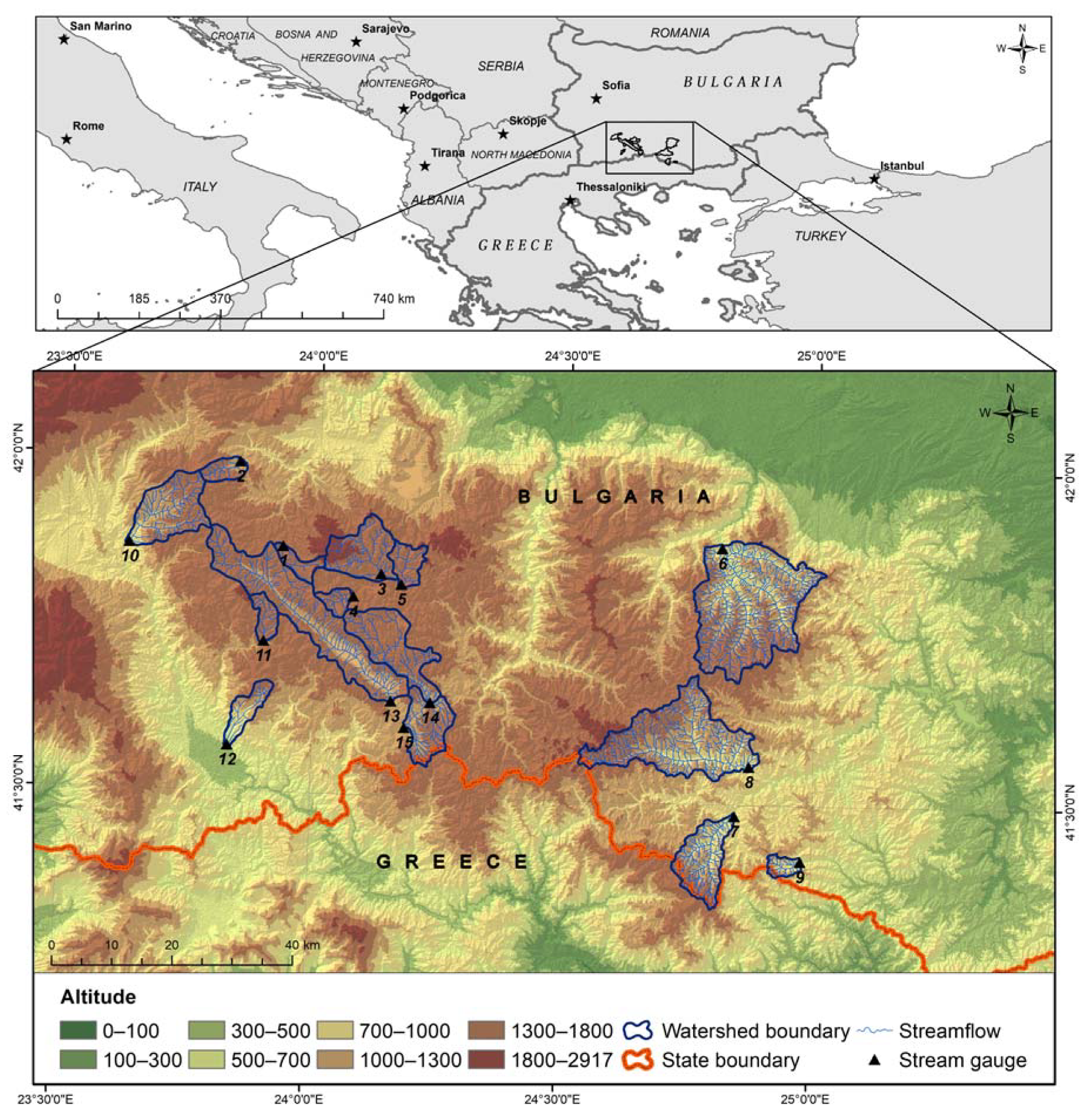
2. Study Area and Datasets Description

The transboundary Rhodope mountain range is a complex system of ridges and deep river valleys extending over 23,500 km2 between longitudes 23°40′ E–26°40′ E and latitudes 40o50′ N–42°15′ N, out of which the 83% is located in Southern Bulgaria, and the remainder 17% in Northern Greece. They are characterised by high-mountainous relief in the western part and low-mountainous and hilly relief in the east/south varying from 0–2191 m with an average elevation of around 630 m. It is notable that the region climate is influenced by both the humid continental climate from the north and by the Mediterranean climate from the south. Furthermore, the average annual temperature varies from 5 to 10 °C in the western part to 13 °C in the eastern and southern parts, whereas the average annual precipitation ranges between 600–1100 mm [42]. The Rhodope Mountain Range is famous for the largest coniferous woods in the Balkans. It includes a number of Bulgarian and Greek Natura 2000 protected sites, whereas a significant part of Bulgaria’s hydropower resources are also located there.
This study employs the flow data inventory from 15 torrential pristine watersheds or watersheds with pre-dam flow regimes that are situated in the study comprises of monthly maximum and mean discharge records, in m3/s, for a time period of at least 10 years of measurement, whereas Figure 1 shows the location of the measuring stations. Moreover, the discharge records were retrieved from hydrological directories that contain data for all gauging stations Bulgaria’s territories, mainly after 1950 [43].
The annual maxima discharges for each station during the time period consists of a fundamental flow information for estimating the peak discharge magnitude for different recurrence intervals. To that end, it is important to know the mean monthly discharge values for the environmental flow estimation. Meanwhile, the mean annual stream discharge was found to range between 0.19 (Dabnitsa gauge) and 5.88 m3/s (Yugovo gauge). Moreover, while seven gauging stations with drainage area ranging between 452–4947 km2 are located in the area, these streams cannot be considered as torrential streams that typically vary from 0.1 to 100 km2 [19] or about 300 km2, according to other studies [17,18]. For this reason, the latter watersheds were excluded from any further analysis.
A total of 25 watershed explanatory variables were calculated and used for the development of the peak discharge and Qenv regional models. To the best of the authors’ knowledge, among them, the length of the straight line from the source to gauging-station (L), the Total stream length (Tl), the circulatory ratio (Rc), the elongation ratio (Re), and the lemniscate ratio (Rl) [44] have been considered for the first time for such purposes, whereas the remaining 20 characteristics have been used in previous regional flood frequency studies and they include the following: Drainage area (A) [1,7,41,45,46,47], Main-channel length (Ls) and Main channel slope (S), [1,7,41,46], Basin length (BL) [7,41,45], Mean basin slope (BS) [46,47], Mean basin elevation (E) [1,7,45,47], Basin Perimeter (B) [41], Mean basin width (BW), Form factor (Rf), Curve factor (Cr), or main-channel sinuosity, accounting the main rivers meandering, gaging-station latitude (GLT) and longitude (GLN) [7], Drainage density (D) [45,47], Compactness ratio (CR), Maximum basin elevation (Emax), Minimum basin elevation (Emin) and Relative basin relief (RH) [47], Basin Relief (H) [45], Basin centroid elevation (CE) [46], and gaging-station elevation (GE) [1].
A spatial database was created to calculate watershed characteristics, which was also inclusive of the digital elevation model (DEM) and the shapefiles of streams, gauging stations, and watershed boundaries. The study area DEM was acquired from a 30 m ASTER- GDEM v.003 data product that does not contain any redistribution requirements on October 2019 [48], whereas the database containing all others elements that were were derived from 1:50,000 scaled topographic maps was provided by the Bulgaria and Greece Ministries of Defence [44]. Moreover, the aforementioned 25 watershed characteristics for the selected 15 watersheds, which were derived from the created database while using simple Geographical Information Systems (GIS) commands in ArcGIS 10.2 software, represent the independent variable utilised in this study. The watersheds encompass a drainage area that ranges from 16 to 326 km2, with basin perimeters from 17.8 to 107.9 km, whereas the main stream length was found to vary between 6 and 50.1 km. The average elevation of all watersheds is above 1000 m, with the average slope exceeding 20%. This, in turn, determines the steep slope of the main channels (from 15.6 to 120.5 m/km). Table 1 summarises the calculated watershed characteristics that were referred to in this study.

3. Materials and Methods

3.1. Peak Flow and Environmental Flow Assessment

In the discharge annual peaks time series, the LP-III probability distribution was fitted to predict the peak flows at selected return periods [21]. Initially, the peak discharge dataset was converted to base 10 logarithms, after which the mean ( log Q ¯ ), the standard deviation ( σ log Q ), as well as the coefficient of skewness ( C s ) of the logarithms of flow were calculated while using the corresponding equations [22]:
log Q ¯ = log Q n
σ log Q = ( log Q log Q ) ¯ 2 n 1
C s = n ( log Q log Q ¯ ) 3 ( n 1 ) ( n 2 ) ( σ log Q ) 3
It is to be noted that the aforementioned three parameters of the LP-III distribution are used to signify the mid-point, the slope, and the curvature of the magnitude frequency curve, respectively [49] Additionally, the flood magnitudes for the storm events occurring during different time periods can be computed by solving equations 4 and 5 [22].
log Q T = log Q ¯ + K σ log Q
Q T = a n t i log ( log Q T )
where log Q T = denotes the base 10 logarithms of the discharge, Q at selected exceedance probability T, whereas K is a factor that is a function of the skew coefficient and selected exceedance probability, which can be obtained while using an appropriate frequency factor Table [21].
The (K-S) and the (A-D) goodness of fit tests were used in order to evaluate whether or not the annual peak flow dataset is consistent with the LP-III distribution. Additional details pertaining to these tests can be found in the research that was conducted by Stephens [50]. In both tests, the null hypothesis is that the dataset follows a specified distribution and that test statistics A2 and D are calculated for the A-D and the K-S tests, respectively. In case the latter statistics are less than the critical value of each test at a chosen significance level, respectively, it can be inferred that the LP-III distribution is suitable for representing the annual daily maximum streamflow distribution in the study area [51]. Additionally, the Weibull plotting position method was only used to graphically illustrate the fitting between the observed and predicted LP-III distribution annual peak discharges [51].
The Tennant [26] method defines different classes of river ecological conditions, so as to protect aquatic life based on the various percentages of the mean annul flow (MAF). A different percentage of the MAF is allocated during the wet and dry periods of the annual corresponding to October–March and April–September, respectively (Table 2). The latter classes range from “Flushing or Maximum” to “Severe Degradation”, whereas, from Table 2, it can be observed that a “Good Habitat” condition is achieved when 40% and 20% of the MAF are allocated for environmental flow during the dry and wet period of the year, respectively. Further details regarding the application of this method can be found in [52].

3.2. Peak Flow and Environmental Flow Regional Models’ Generation

At the initial states, independent variables were transformed to Z-scale standardised values with a mean and standard deviation equal to 0 and 1, respectively, in order to ensure that the latter variables had equal weights during the PCA analysis. Additional details regarding this process can be found in [53]. The second issue to be addressed is with respect to the correlation strength between the variables for the PCA analysis to be applicable, which can be derived by calculating the Bartlett’s test of sphericity [54] and the Kaiser-Meyer-Olkin (KMO) measure of sampling adequacy [55] statistical measures. Bartlett’s test of Sphericity should be statistically significant at p < 0.05, and the KMO value for the multiple variables should be 0.6 or above to ensure good factor analysis [28]. Further details regarding the two aforementioned statistics can be found in [56]. Additionally, the KMO can also be calculated for each separate variable, while individual variables with KMO values of less of less than 0.5 were excluded from the PCA analysis [34].
The PCA method with varimax rotation is the most commonly used approach, so as to decide whether or not a factor is statistically important [28]. Additionally, it simplifies the interpretation of the factors [34]. PCA analysis generates a new set of factor as linear composites of the original variables, referred to as Principal Components (PCs) [57], whereas PC1 denotes that the linear combination of the original variables, which contributes a maximum to their total variance; in a similar vein, PC2 contributes a maximum to the residual variance, and so on, until the analysis of the total variance [53]. The number of PCs accounted was chosen based on the Kaiser criterion, according to which only PC with eigenvalues greater than 1 should be retained in the analysis [58]. Moreover, only factor loadings with absolute values of above 0.75 (depicting a strong correlation between a specific observed variable and a PC) were selected [56]. Meanwhile, the subsequent step of the PCA analysis entailed the residuals examination between the observed correlations and the reproduced correlations that are based on the model; less than 50% of the residuals must have absolute values that are in excess of 0.05, so as to presume a good model fit [34,57].
The purpose of multiple linear regression (MLR) analysis is to fit a predictive model to the data from a set of several independent variables and then to use that model to predict the values of the dependent variable [34]. The use of a regression model to predict a result and then compare this result with some independent measurements is the most common mistake that is made in regional regression modeling process. This is because it actually creates a second model that relates the observed and predicted values to each other [59]; thus, it was decided to not divide the watershed inventory into model development and validation subsets. Furthermore, oftentimes, relationships may not be linear in watershed, hydrology, and ecological studies [59]. In this study, linear (Εquation (6)), the power (Εquation (7)), exponential (Εquation (8)), and logarithmic models (Εquation (9)) were assessed so as to generate the relationships between each dependent variable with the explanatory variables that were derived from the PCA analysis. The latter model combination has been used for other purposes, such as for identifying the relationships between concentration-discharge and load-discharge [60], but not to derive models for forecasting peak discharge at selected recurrence intervals and environmental flows.
y = a + b 1 x 1 + b 2 x 2 + ..... b i x i
y i = a * x 1 b 1 * x 2 b 2 * ........ * x i b i
y = a e b 1 x 1 e b 2 x 2 ..... e b i x i
y = a + b 1 ln ( x 1 ) + b 2 ln ( x 2 ) + ..... b i L n ( x i )
where yi denote the dependent variable, xi signifies the explanatory variables, a is constant, bi, b2... bi are the regression coefficients for each independent variable, and i represents the number of explanatory variables. While making use of appropriate mathematic transformation techniques, it is possible to shift the power, the exponential, and the logarithmic models into multiple linear models, and their explanatory coefficients values can be subsequently computed by applying stepwise multiple regression analysis [45,61]. Moreover, the latter MLR models can be retransformed to their original prediction equation form by using similar mathematic transformation techniques [1].
The regional models evaluation was achieved by utilising the statistic measures of the coefficient of determination (R2), the Root mean square error (RMSE), the prediction error (PE), or the Mean Absolute Percent Error (MAPE), the Nash–Sutcliffe efficiency (NSE), as well as the index of agreement (d), which have also been used in similar studies [40,41,62,63]. Meanwhile, the relevant equations are, respectively, expressed, as follows:
R 2 = ( ι 1 n ( O i O ¯ ) * ( P i P ¯ 2 ) i = 1 n ( O i O ¯ ) 2 * i = 1 n ( P i P ¯ ) 2 ) 2 ,     0 R 2 1
R M S E = ι = 1 n ( P i O i ) 2 n ,       0 P E
P E = n 1 * i = 1 n | ( O i P i ) / O i | * 100 ,     0 P E
N S E = 1 i = 1 n ( O i P i ) 2 i = 1 n ( O i O ¯ ) 2 ,     E 1
d = 1 i = 1 n ( O i P i ) 2 i = 1 n ( | P i O ¯ | + | O i O ¯ | ) 2 , 0 d 1
where Oi and Pi are the measured and predicted values, respectively, of the under study variable at time i, O ¯ and P ¯ denote the mean values of the observed and predicted variable, whilst n signifies the number of records. The closest the values of the R2, NSE, and d to 1, the better the association between measured and predicted variables. On the other hand, an NSE value of lower than zero indicates that the mean value of the observed time series would have been a better predictor than the model [64]. Moreover, the closer the values of the RMSE and PE statistics are to zero, the better the model’s predictions fits the observations. Finally, the multiple regional models’ development was conducted through the use of IBM SPSS Version 23 software, whereas the computation of five statistical evaluation measurers was performed while utilising an online calculator tool [65].

4. Results and Discussion

4.1. Peak Flow and Environmental Flow Computation

The LP-III distribution was adjusted to the annual maxima discharge time series while using a simple spreadsheet, in which the relevant data and equations were incorporated. The annual peak flow series for the 15 stream gauges have a record length ranging from 10 to 28 years and was computed using a simple mathematic function. The 10 years of peak-flow record from pristine catchments are considered to be sufficient for continuously performing a regression analysis [7]. Additionally, the mean, the standard deviation, and the skewness coefficient of discharge annual peaks time series logarithms for the different recurrence intervals were computed in accordance with the Water Resources Council [21] guidelines. The expected design flood discharges were calculated for 25, 50, and 100 years return periods by solving equations 4 and 5, whereas Table 3 illustrates the emerging results in cubic hectometre per year (hm3/year).
At some watersheds, the Q25, Q50, and Q100 values computed by the LP-III distribution differ a little. Meanwhile in similar studies, such as in the Minab river at Iran [66] or the Mahi river in India [49], a similar small difference has been observed, which could be attributed to the fact that the discharge might be dominated by groundwater flows or the rain shadow effect. The observed and the predicted LP-III distribution annual peak discharges for all cases were observed to be fairly close to most of the data points. For this reason, the predicted discharge values are likely to be quite reliable [49]. Figure 2 illustrates a reasonable fit between the observed and predicted LP-III distribution annual peak discharges for a random gauge, Velingrad. Moreover, the statistic values for the K-S and A-D goodness of fit tests were computed based on [50] guidelines, whilst the critical value at a 95% confidence level for the K-S test were found to range between 0.257 and 0.410, while the critical value was 2.502 for the A-D test. It can be inferred that the LP-III distribution is appropriate enough to represent the annual daily maximum streamflow distribution, since it can be seen from Table 3 that the maximum value of the K-S and the A-D statistics were calculated equal to 0.21 and 0.76 respectively, which is less than the aforementioned critical values.
Regarding the Qenv assessment that was based on Tennant’s [26] method, the MAF for the 15 under study catchments were initially computed, whereas the river ecological condition corresponding to “Poor or minimum” habitat conditions was selected as the desired ecosystem condition for this study. Under the latter habitat condition, a 10% proportion of the MAF, which corresponds to a minimum river depth and minimum average flow velocity of 0.3 m must be 0.25 m/s, respectively [27], is allocated in the river during the entire year to sustain short-term aquatic life. The 10% percentage of the MAF that is necessary for maintaining the minimum ecosystem attributes constituted the Qenv variable. Table 3 summarises the results that were derived from the application of this method. The Qenv magnitude was found to range from 18.55 hm3/year for the Yugovo watershed to 0.61 hm3/year for the Dabnitsa watershed in order to maintain minimum habitat conditions in the study area. The latter values correspond to 50,811 and 1,665 m3/day, respectively.

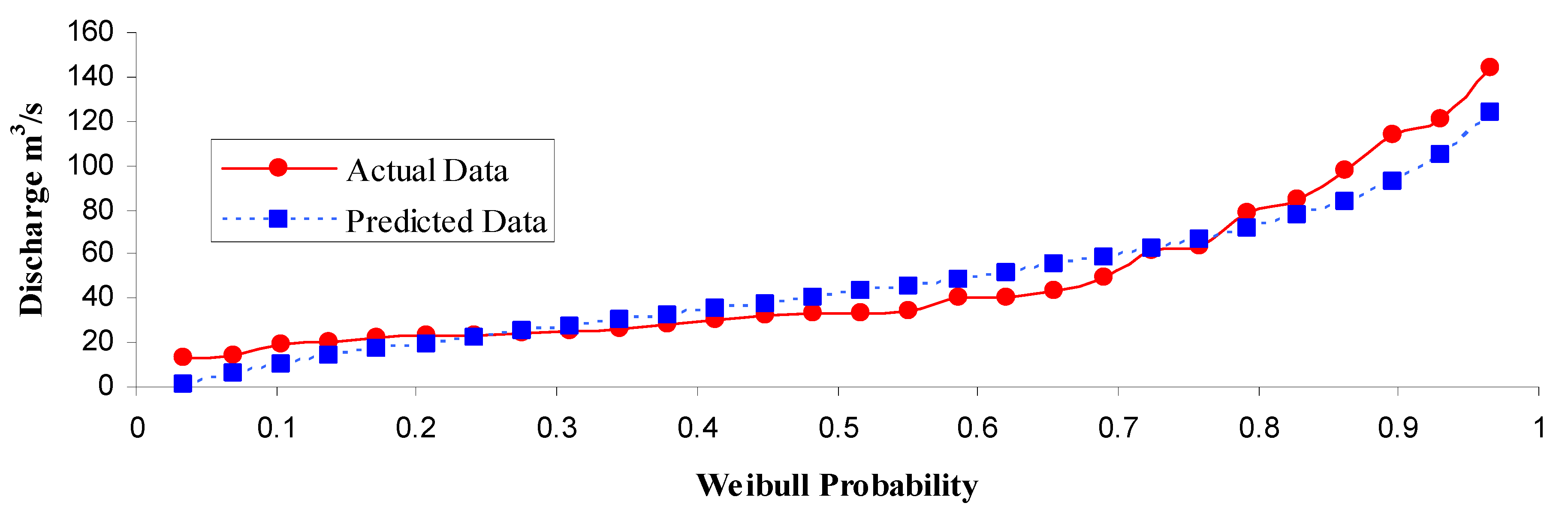
4.2. Hydrologic and Sediment Yield Modeling

The 25 independent variables were standardised [53] and all of the individual variables with a KMO value of less than 0.5 were omitted from the analysis, which resulted in the following 16 variables: B, L, Ls, BL, A, Tl, Emax, BW, S (H/Ls), Rc, E, BS, CE, GE, Emin, and GLN. None of the latter variables had an individual KMO value of less than 0.6. The overall mean KMO value of all variables was computed equal to 0.715, which suggested that there is a middling adequacy of the correlations between the variables [57]. Meanwhile, the Barlett test value was found to be equal to 0.000, which also indicated that there are significant correlations among variables, which is why it is valid to proceed with the PCA analysis [28,34].
After the PCA, analysis with varimax rotation was applied to the latter 16 variables, and it was found that only the first component (PC1) and the second component (PC2) had an eigenvalues of greater than 1, while the two components cumulative explained 83.3% of the total variance (53.8% the PC1 and 29.5% the PC2). Jenicek et al. [67] also posits that PCs, which explain a little variance, can be removed with a minimum loss of explanatory power of the original dataset. The PC1 comprises of 10 items with absolute loading values that ranged from 0.96 to 0.68 and it is primarily connected with the watershed morphometric characteristics. On the other hand, the PC2 consists of six items with absolute loading values ranging from 0.92 to 0.67 and mainly expressing the watershed hypsometric features influence (Table 4). Additionally, the residuals between the observed and reproduced correlations were computed where 25 (20.0%) non-redundant residuals were found with absolute values that were greater than 0.05, thus confirming a well-suited model [57].
Table 4 shows that the Rc and the GLN variables have factor loading with absolute values that were below the 0.75 threshold, which suggests that they could be excluded from further analysis [56]. Therefore, after PCA analysis was rerun without the latter two variables, it was noted the PC1 and the PC2 account for 65.1% and the 23.9%, respectively, of the overall variance, cumulative of 89.0% of the total variance. Meanwhile, the residuals between the observed and reproduced correlations were decreased to 13 (14.0%) non-redundant residuals with absolute values greater than 0.05, thus denoting a better model ft when these two factors were discarded from further analysis. Sharma et al. also reported the increase in the total variance explicated by PCA by screening out the variables with poor correlation [68].
The relationships between each dependent variable (Q25. Q50, Q100, and Qenv) with the 14 explanatory variables derived from the PCA analysis (B, L, Ls, BL, A, Tl, Emax, BW, S, E, BS, CE, GE, and Emin) for the four different model types were calculated through application of the stepwise multiple regression analysis, [40,46], which reduces the number of explanatory variables to those significant at the 95% confidence level [35]; Table 5 illustrates the relevant results, where it can be observed that that the linear models and logarithmic models exhibit the worst and the second worst prediction efficiency, respectively, for the peak discharge values prognosis concerning the selected recurrence intervals with low R2 and high PE, in comparison to the power or exponential models. Although the power and exponential model yielded similar results for the Q25 forecast in terms of the R2, RMSE, NSE, and d statistical measures, the exponential model was found to have a smaller PE value, and it should be selected for the discharge value with 25 years recurrence interval assessment. However, the power models clearly outperformed all other types of models for the Q50 and Q100 prediction, since they depicted not only the highest R2, d, and NSE values, but also the smaller PE and RMSE values. Finally, although the linear and power models illustrated the same fit for the Qenv prediction, the linear model has a slightly better prediction than the power model, since it depicts larger NSE and d and smaller RMSE values.
According to the regression analysis, the explanatory variables in which the peak discharge prediction with a 25 recurrence interval is based are as follows: gauging station elevation (GE) and the length of the straight line from source to gauging-station (L). On the other hand, the Q25 and Q100 prediction is also premised on the latter variables plus the drainage area (A). The length (L) of the main river course from the divide of the basin to the measuring station and the drainage area (A) has also been indicated in similar peak flow regression analysis studies, as determinant explanatory variables in order to compute peak discharge values for different return periods [7,32,41]. However, to the best of the authors’ knowledge, it is the first time that the gauge station elevation (GE) is found to be a significant determinant, despite having been assessed by [1]. Moreover, this research highlighted the total stream length (TI) as a determinant factor for environmental flow estimation that has not been assessed in similar regression analysis studies for environmental flows computation at ungauged basins [35,60].
Notably, the four regional equation models’ performance marked a high forecasting accuracy for the dependent variables by the explanatory variables, since the R2, the NSE, and the d were found to range from 0.91–0.96, 0.88–0.95, and 0.97–0.99, respectively. Mimikou [40] also reported R2 values that were equal to 0.96 and 0.98 for the maximum observed floodflows for the western and north western region of Greece, respectively, whereas Selvanathan et al. [46] developed regression equations that relate peak discharges to basin and climate characteristics with an accuracy reaching an R2 values equal to 0.86 for certain regions of the U.S. El-Jabi and Caissie [69] developed regional models for mean, median, high, as well as low flows of different recurrence intervals in New Brunswick with high R2 values ranging between 0.799 and 0.989. On the other hand, Zhang et al. [35] developed a regression equation for computing environmental flow with an adjusted R2 value of 0.96. Moreover, the emerging equations for the Q25, Q50, Q100, and Qenv projection in this study illustrate a prediction error (PE) between 24.20 and 39%, which is in alignment with the findings of similar studies, such as Topaloúlu [41], who reported PE values between 20.24–34.07 or Antonopoulos et al. [60], who found MAPE values that ranged between 23.8 and 43.8. Finally, since many regions of the world are experiencing more intense rainfall as well as more frequent flooding/drought with each passing decade due to global climate change methods such as this, it can be inferred that stationarity should only be used as a guideline.

5. Conclusions

This study confirmed the notion that regionalisation techniques use produces reliable models that are suitable for predicting peak discharge with 25, 50, and 100 years return periods and environmental flows with great accuracy, whereas the latter information is absolutely necessary for water resources management projects, and hydrologic and hydraulic design. The selected 25 watershed characteristics were calculated for 15 pristine watersheds in the region using standard GIS methods and they represented the independent model variables, whereas PCA analysis reduced the explanatory variables number to 14. Additionally, the peak flows with annual probabilities 1/25, 1/50, and 1/100 were computed by fitting the LP-III distribution while using a streamflow historic records dataset with at least 10 years timespan, whilst the Qenv magnitude was assessed by the Tennant method and it represented the model dependent variables.
The stepwise multiple regression analysis was performed to derive the relationships between the dependent and independent variables and it was found that the gauging-station elevation, the length of the straight line from source to gauging-station, as well as the drainage area were the most significant explanatory variables in explaining peak flows, while the total stream length was the parameter that described Qenv. The exponential model was found most suitable for predicting Q25, the power model was deemed most feasible for forecasting Q50 and Q100, whereas the linear model was found to prognose Qenv in the best possible manner. Furthermore, four statistical evaluation measures revealed the emerged models’ high accuracy of the obtained models. The developed regional peak-flow and environmental flows models could be employed in an ungauged unregulated watershed within broader regions in the Rothope Mountain Range to calculate the peak discharge magnitude with 25, 50, and 100 year return periods, respectively and the Qenv by determining the required watershed characteristics to apply the equations obtained. However, these watershed characteristics should be within the range of characteristics that were initially used to develop the regional models.

Author Contributions

In this research, E.I. computed the explanatory and depended variables, whereas D.M. generated and evaluate the regional models. Meanwhile, both authors equally contributed to the study design and the discussion of results. All authors have read and agreed to the published version of the manuscript.

Funding

This research received no external funding.

Acknowledgments

Part of the present research was conducted during D. Myronidis Erasmus+ Staff Mobility for training mission in the Space Research and Technology Institute (SRTI) research unit of the Bulgarian Academy of Sciences (BAS) between 28/10–01 and 11/2019. The authors would like to sincerely thank the two anonymous experts along with the editor for their time and constructive comments that helped improve this paper substantially as a result of their feedback.

Conflicts of Interest

The authors declare no conflict of interest.

References

  1. Campbell, A.J.; Sidle, R.C. Prediction of peak flows on small watersheds in Oregon for use in culvert design. J. Am. Water Resour. As. 1984, 20, 9–14. [Google Scholar] [CrossRef]
  2. Myronidis, D.; Stathis, D.; Sapountzis, M. Post-Evaluation of Flood Hazards Induced by Former Artificial Interventions along a Coastal Mediterranean Settlement. J. Hydrol. Eng. 2016, 21, 05016022. [Google Scholar] [CrossRef]
  3. Myronidis, D.; Fotakis, D. Utilizing 3D solid modeling tools for simplified designing of a small concrete Gravity Dam. IJSAMI 2015, 1, 351–357. [Google Scholar] [CrossRef]
  4. Myronidis, D.; Emmanouloudis, D.; Arampatzis, G. Research on the contribution of Small Hydroelectric Plants (SHP) as development projects to the energy balance of Greece. J. Environ. Prot. Ecol. 2008, 9, 614–626. Available online: https://docs.google.com/a/jepe-journal.info/viewer?a=v&pid=sites&srcid=amVwZS1qb3VybmFsLmluZm98amVwZS1qb3VybmFsfGd4OjY4ZGU3YWM4NGMzNmQxODg (accessed on 12 February 2020).
  5. Castellarin, A.; Kohnová, S.; Gaál, L.; Fleig, A.; Salinas, J.L.; Toumazis, A.; Kjeldsen, T.R.; Macdonald, N. Review of Applied-Statistical Methods for Flood-Frequency Analysis in Europe. Cost Action ES0901, Working Group 2 Report. 2012, pp. 1–130. Available online: http://nora.nerc.ac.uk/id/eprint/19286 (accessed on 12 February 2020).
  6. Myronidis, D.; Ioannou, K. Forecasting the Urban Expansion Effects on the Design Storm Hydrograph and Sediment Yield using Artificial Neural Networks. Water 2019, 11, 31. [Google Scholar] [CrossRef] [Green Version]
  7. Hodgkins, G.A.; Martin, G.R. Estimating the Magnitude of Peak Flows for Streams in Kentucky for Selected Recurrence Intervals. U.S. Geological Survey, Water-Resources Investigations. Report 3–4180; 2003. Available online: https://www.google.com/url?sa=t&rct=j&q=&esrc=s&source=web&cd=1&ved=2ahUKEwjRzpvO0svnAhWDzKQKHd0nCO0QFjAAegQIAxAB&url=https%3A%2F%2Fpubs.usgs.gov%2Fwri%2Fwri034180%2Fpdf%2Fwri034180.pdf&usg=AOvVaw0-YS5RR1NbgKAKP68QE2B9 (accessed on 12 February 2020).
  8. Richter, B.D.; Baumgartner, J.V.; Powell, J.; Braun, D.P. A method for assessing hydrologic alteration within ecosystems. Conserv. Biol. 1996, 10, 1163–1174. [Google Scholar] [CrossRef] [Green Version]
  9. Gleick, P.H.; Allen, L.; Christian-Smith, J.; Cohen, M.J.; Cooley, H.; Heberger, M.; Morrison, J.; Palaniappan, M.; Schulte, P. The World’s Water Volume 7-the Biennial Report on Freshwater Resources; Island Press: Washington, DC, USA, 2012; pp. 1–440. [Google Scholar] [CrossRef] [Green Version]
  10. Rodell, M.; Famiglietti, J.S.; Wiese, D.N.; Reager, J.T.; Beaudoing, H.K.; Landerer, F.W.; Lo, M.H. Emerging trends in global freshwater availability. Nature 2018, 557, 651–659. [Google Scholar] [CrossRef]
  11. Tharme, R.E. A global perspective on environmental flow assessment: Emerging trends in the developments and applications of environmental flow methodologies for rivers. River Res. Appl. 2003, 19, 397–441. [Google Scholar] [CrossRef]
  12. Pastor, A.V.; Ludwig, F.; Biemans, H.; Hoff, H.; Kabat, P. Accounting for environmental flow requirements in global water assessments. Hydrol. Earth Syst. Sci. 2014, 18, 5041–5059. [Google Scholar] [CrossRef] [Green Version]
  13. Linnansaari, T.; Monk, W.A.; Baird, D.J.; Curry, R.A. Review of Approaches and Methods to Assess Environmental Flows across Canada and Internationally. Canadian Science Advisory Secretariat, Research Document 2012/039. 2012. Available online: https://www.google.com/url?sa=t&rct=j&q=&esrc=s&source=web&cd=2&ved=2ahUKEwjShtSHpJLoAhXLzMQBHc7jAwAQFjABegQICRAB&url=https%3A%2F%2Fwaves-vagues.dfo-mpo.gc.ca%2FLibrary%2F348885.pdf&usg=AOvVaw1b6Qu0-J3o9eXDuEp3Jgs7 (accessed on 11 March 2020).
  14. Ramos, V.; Formigo, N.; Maia, R. Ecological flows and the Water Framework Directive implementation: An effective coevolution? Eur. Water 2017, 60, 423–432. Available online: https://www.google.com/url?sa=t&rct=j&q=&esrc=s&source=web&cd=1&ved=2ahUKEwiUpOKztsznAhWEolwKHRh5CpIQFjAAegQIBBAB&url=https%3A%2F%2Fwww.ewra.net%2Few%2Fpdf%2FEW_2017_60_58.pdf&usg=AOvVaw0WNELSglMQCdJAs5eym3cf (accessed on 12 February 2020).
  15. E.U. Ecological Flows in the Implementation of the Water Framework Directive; Technical Report 086; Office for Official Publications of the European Communities: Luxembourg, 2015; Available online: https://www.google.com/url?sa=t&rct=j&q=&esrc=s&source=web&cd=1&ved=2ahUKEwiu7Y_YtsznAhVbi1wKHdyZAF8QFjAAegQIBhAB&url=https%3A%2F%2Fcircabc.europa.eu%2Fsd%2Fa%2F4063d635-957b-4b6f-bfd4-b51b0acb2570%2FGuidance%2520No%252031%2520-%2520Ecological%2520flows%2520%2528final%2520version%2529.pdf&usg=AOvVaw0Cg-qtzKRjzl_ebqNrFTN8 (accessed on 12 February 2020).
  16. Patsialis, T.; Skoulikaris, C.H.; Ganoulis, J. Ecological Flow for Integrated Planning of Small Hydropower Plants: A Case Study from Greece. In Proceedings of the FRIEND-Water, Hanoi, Vietnam, February 2014; Available online: https://iahs.info/uploads/dms/16633.84-469-474-363-13-Paper-98-Patsialis-et-al.pdf (accessed on 11 March 2020).
  17. Kotoulas, D. Management of Torrents; Publication of the Aristotle University of Thessaloniki: Thessaloniki, Greece, 1997; pp. 1–669. (In Greek) [Google Scholar]
  18. Iliadis, L.; Maris, F.; Tsataltzinos, T. An Innovative Decision Support System Using Fuzzy Reasoning for the Estimation of Mountainous Watersheds Torrential Risk: The Cases of Lakes Koroneia and Volvi. In Proceedings of the IUFRO Conference, Edinburgh, Scotland, 2018; Available online: https://nanopdf.com/download/an-innovative-decision-support-system-using-fuzzy-reasoning-for-the-mountainous_pdf (accessed on 11 March 2020).
  19. Ancey, C. Debris flows. In Environmental Geomechanics; Delage, P., Schrefler, B., Eds.; John Wiley & Sons: Hoboken, NJ, USA, 2013. [Google Scholar]
  20. Ristić, R.; Kostadinov, S.; Abolmasov, B.; Dragićević, S.; Trivan, G.; Radić, B.; Trifunović, M.; Radosavljević, Z. Torrential floods and town and country planning in Serbia. Nat. Hazards Earth Syst. Sci. 2012, 12, 23–35. [Google Scholar] [CrossRef]
  21. Water Resources Council. Guidelines for Determining Flood Flow Frequency–Bulletin 17B of the Hydrology Subcommittee. U.S. Geological Survey, Office of Water-Data Coordination, 1982; 183p. Available online: https://www.google.com/url?sa=t&rct=j&q=&esrc=s&source=web&cd=2&ved=2ahUKEwi11Lyzgs7nAhVIiqQKHZoRDnMQFjABegQIBBAB&url=https%3A%2F%2Fwater.usgs.gov%2Fosw%2Fbulletin17b%2Fdl_flow.pdf&usg=AOvVaw2XGH_z_q5WHOLNT-95ViHD (accessed on 12 February 2020).
  22. Mays, L.W. Water Resources Engineering, 2nd ed.; Wiley & Sons: Hoboken, NJ, USA, 2010; pp. 1–920. [Google Scholar]
  23. Amin, M.T.; Rizwan, M.; Alazba, A.A. A best-fit probability distribution for the estimation of rainfall in northern regions of Pakistan. Open Life Sci. 2016, 11, 432–440. [Google Scholar] [CrossRef]
  24. Kamal, V.; Mukherjee, S.; Singh, P.; Sen, R.; Vishwakarma, C.A.; Sajadi, P.; Asthana, H.; Rena, V. Flood frequency analysis of Ganga river at Haridwar and Garhmukteshwar. Appl. Water Sci. 2017, 7, 1979–1986. [Google Scholar] [CrossRef] [Green Version]
  25. Toranjian, A.; Marofi, S. Evaluation of statistical distributions to analyze the pollution of Cd and Pb in urban runoff. Water Sci. Technol. 2017, 75, 2072–2082. [Google Scholar] [CrossRef]
  26. Tennant, D.L. Instream Flow Regimens for Fish, Wildlife, Recreation and Related Environmental Resources. Fisheries 1976, 1, 6–10. [Google Scholar] [CrossRef]
  27. Karakoyun, Y.; Dönmez, A.H.; Yumurtac, Z. Comparison of environmental flow assessment methods with a case study on a runoff river–type hydropower plant using hydrological methods. Environ. Monit. Assess 2018, 12, 722. [Google Scholar] [CrossRef]
  28. Pallant, J. SPSS Survival Manual: A Step by Step Guide to Data Analysis Using Spss; Open University Press/McGraw-Hill 2: London, UK, 2010; pp. 1–33. [Google Scholar]
  29. Griffis, V.W.; Stedinger, J.R. The use of GLS regression in regional hydrologic analyses. J. Hydrol. 2007, 344, 82–95. [Google Scholar] [CrossRef]
  30. Maris, F.; Kitikidou, K.; Paparrizos, S.; Potouridis, S. Stream flowquantile regression modelling using land use information in the Sperchios river basin (Central Greece). Carpath J. Earth Environ. 2014, 9, 5–10. Available online: http://www.ubm.ro/sites/CJEES/viewTopic.php?topicId=390 (accessed on 12 February 2020).
  31. Mimikou, M. Regional relationships between basin size and runoff characteristics. Hydrolog. Sci. J. 1984, 29, 63–73. [Google Scholar] [CrossRef] [Green Version]
  32. Mimikou, M.; Gordios, J. Predicting the mean annual flood and flood quantiles for ungauged catchments in Greece. Hydrolog. Sci. J. 1989, 34, 169–184. [Google Scholar] [CrossRef]
  33. IBM Corp. Released IBM SPSS Statistics for Windows; Version 23.0; IBM Corp: Armonk, NY, USA, 2015. [Google Scholar]
  34. Field, A. Discovering Statistics Using SPSS, 2nd ed.; Sage Publications: Southend Oaks, CA, USA, 2005; pp. 1–816. [Google Scholar]
  35. Zhang, Z.; Balay, J.W.; Bertoldi, K.M.; MaCoy, P.O. Assessment of Water Capacity and Availability from Unregulated Stream Flows Based on Ecological Limits of Hydrologic Alteration (ELOHA) Environmental Flow Standards. River Res. Appl. 2016, 32, 1469–1480. [Google Scholar] [CrossRef]
  36. Daniil, Ε.Ι.; Michas, S.N.; Nikolaou, K.; Lazaridis, L.S. Systematic approach for ungaged basins’ discharge determination in Western Peloponnese, Greece. Glob. Nest J. 2012, 14, 344–353. Available online: https://www.google.com/url?sa=t&rct=j&q=&esrc=s&source=web&cd=2&ved=2ahUKEwiio_Dhi87nAhVJuqQKHWK8B38QFjABegQIAhAB&url=https%3A%2F%2Fjournal.gnest.org%2Fsites%2Fdefault%2Ffiles%2FJournal%2520Papers%2F344-353_878_DANIIL_14-3.pdf&usg=AOvVaw1mz_zfpPq7cKh9Th4EBwDl (accessed on 12 February 2020).
  37. Borisova, D.; Aydarova, Z.; Stefanov, S.; Hristova, N. Extreme values of the flow in the Maritza River Basin (Pazardzhik) for the period 2000–2005 (in Bulgarian). Probl. Geogr. 2015, 1–2, 185–197. [Google Scholar]
  38. Hristova, N. Statistical analysis of low flow for Archar River Basin. Dir. Sofia Univ. St. Kliment Ohridski 2016, 107, 25–38. [Google Scholar]
  39. Gerassimov, S.; Bojilova, E. River basin management, Bulgarian case study. Phys. Chem. Earth 2008, 33, 395–402. [Google Scholar] [CrossRef]
  40. Mimikou, M. Regional analysis of hydrological variables in Greece. In Regionalization in Hydrology Proceedings of the Ljubljana Symposium, Ljubljana, Slovenia, April 1990; No. 191; IAHS Publication: Wallingford, UK, 1990. [Google Scholar]
  41. Topaloúlu, F. Estimation of Instantaneous Peak Flows in Seyhan River Basin Using Regional Regression Procedures. Turk. J. Agric. For. 2002, 26, 47–55. Available online: https://journals.tubitak.gov.tr/agriculture/issue.htm?id=400 (accessed on 12 February 2020).
  42. Yordanova, M.; Velev, S.; Drenovski, I. Characteristic features of the physical geographical regions. In Geography of Bulgaria: Physical and Socio-Economic Geography; Kopralev, I., Ed.; BAS: Sofia, Bulgaria, 2002. [Google Scholar]
  43. BAS. Reference Book of the Rivers in the People’s Republic of Bulgaria; Bulgarian Academy of Sciences; Institute of Meteorology and Hydrology: Sofia, Bulgarian, 1981. (In Bulgarian) [Google Scholar]
  44. Ivanova, E.K.; Nedkov, R.D.; Ivanova, I.B.; Radeva, K.L. Morpho-hydrographic analyze of Black Sea Catchment Area in Bulgaria. Procedia Environ. Sci. 2012, 14, 143–153. [Google Scholar] [CrossRef] [Green Version]
  45. Pitlick, J. Relation between peak flows, precipitation, and physiography for five mountainous regions in the western USA. J. Hydrol. 1994, 158, 219–240. [Google Scholar] [CrossRef]
  46. Selvanathan, S.; Sreetharan, M.; Rand, K.; Smirnov, D.; Choi, J.; Mampara, M. Developing peak discharges for future flood risk studies using IPCC’s cmip5 climate model results and USGS WREG program. J. Am. Water Resour. As. 2016, 52, 979–992. [Google Scholar] [CrossRef]
  47. Ahn, K.H.; Palmer, R. Regional flood frequency analysis using spatial proximity and basin characteristics: Quantile regression vs. parameter regression technique. J. Hydrol. 2016, 540, 515–526. [Google Scholar] [CrossRef]
  48. NASA. ASTER Global Digital Elevation Model Version 3, National Aeronautics and Space Administration (NASA). Available online: https://asterweb.jpl.nasa.gov/ (accessed on 12 February 2020).
  49. Pawar, D.C.; Hire, P. Flood Frequency Analysis of the Mahi Basin by Using Log Pearson Type III Probability Distribution. Hydrospatial Anal. 2018, 2, 102–112. [Google Scholar] [CrossRef] [Green Version]
  50. Stephens, M.A. EDF Statistics for Goodness of Fit and Some Comparisons. J. Am. Stat. Assoc. 1974, 69, 730–737. [Google Scholar] [CrossRef]
  51. Abdullah, J.; Muhammad, N.S.; Mohamad Sharif, N.A. Estimation of Peak Discharges Using Flood Frequency Analysis and Hydrological Modeling System. In Proceedings of the International Symposium on Flood Research and Management; Tahir, W., Abu, B.P., Wahid, M., Mohd, N.S., Lee, W., Eds.; Springer: Singapore, 2015; pp. 129–139. [Google Scholar]
  52. Liu, J.; Liu, Q.; Yang, H. Assessing water scarcity by simultaneously considering environmental flow requirements, water quantity, and water quality. Ecol Indic. 2016, 60, 434–441. [Google Scholar] [CrossRef] [Green Version]
  53. Singh, P.K.; Kumar, V.; Purohit, R.C.; Kothari, M.; Dashora, P.K. Application of principal component analysis in grouping geomorphic parameters for hydrologic modelling. Water Resour. Manag. 2009, 23, 325–339. [Google Scholar] [CrossRef]
  54. Bartlett, M.S. A note on the multiplying factors for various chi square approximations. J. R. Stat. Soc. 1954, 16, 296–298. Available online: https://www.jstor.org/stable/2984057 (accessed on 12 February 2020).
  55. Kaiser, H. An index of factorial simplicity. Psychometrika 1974, 39, 31–36. [Google Scholar] [CrossRef]
  56. Azid, A.; Juahir, H.; Toriman, M.E.; Kamarudin, M.K.A.; Saudi, A.S.M.; Hasnam, C.N.C.; Aziz, N.A.A.; Azaman, F.; Latif, M.T.; Zainuddin, S.F.M.; et al. Prediction of the level of air pollution using principal component analysis and artificial neural network techniques: A case study in Malaysia. Water Air Soil Pollut. 2014, 225, 2063. [Google Scholar] [CrossRef]
  57. Mooi, E.; Sarstedt, M.A. Concise Guide to Market Research: The Process, Data, and Methods Using Ibm Spss Statistics; Springer: Berlin/Heidelberg, Germany, 2011. [Google Scholar] [CrossRef]
  58. Wiatkowski, M.; Wiatkowska, B. Changes in the flow and quality of water in the dam reservoir of the Mała Panew catchment (South Poland) characterized by multidimensional data analysis. Arch. Environ. Prot. 2019, 45, 26–41. [Google Scholar] [CrossRef]
  59. Ward, A.D.; Trimble, S.W. Environmental Hydrology, 2nd ed.; Lewis Publishers: Boca Raton, FL, USA, 2004; pp. 1–475. [Google Scholar]
  60. Antonopoulos, V.Z.; Papmichail, D.M.; Mitsiou, K.A. Statistical and trend analysis of water quality and quantity data for the Strymon River in Greece. Hydrol. Earth Syst. Sci. 2001, 5, 679–691. [Google Scholar] [CrossRef]
  61. Amiri, B.J.; Gao, J.; Fohrer, N.; Adamowski, J. Regionalizing time of concentration using landscape structural patterns of catchments. J. Hydrol. Hydromech. 2019, 67, 135–142. [Google Scholar] [CrossRef] [Green Version]
  62. Koutroulis, A.G.; Tsanis, I.K. A method for estimating flash flood peak discharge in a poorly gauged basin: Case study for the 13–14 January 1994 flood, Giofiros basin, Crete, Greece. J. Hydrol. 2010, 385, 150–164. [Google Scholar] [CrossRef]
  63. Nanos, N.; Sjöstedt de Luna, S. Fitting diameter distribution models to data from forest inventories with concentric plot design. For. Syst. 2017, 26. Available online: http://revistas.inia.es/index.php/fs/article/view/10486/3630 (accessed on 12 February 2020). [CrossRef] [Green Version]
  64. Alexakis, D.; Grillakis, M.G.; Koutroulis, A.G.; Agapiou, A.; Themistocleous, K.; Tsanis, I.; Michaelides, S.; Pashiardis, S.; Demetriou, C.; Aristeidou, K.; et al. GIS and remote sensing techniques for the assessment of land use change impact on flood hydrology: The case study of Yialias basin in Cyprus. Nat. Hazard Earth Syst. 2014, 14, 413–426. [Google Scholar] [CrossRef] [Green Version]
  65. AgriMetSoft Online Calculators. Available online: https://agrimetsoft.com/calculators/Root%20Mean%20Square%20Error (accessed on 12 February 2020).
  66. Khosravi, G.H.; Majidi, A.; Nohegar, A. Determination of Suitable Probability Distribution for Annual Mean and Peak Discharges Estimation (Case Study: Minab River- Barantin Gage, Iran). Int. J. Probab. Stat. 2012, 1, 160–163. [Google Scholar] [CrossRef] [Green Version]
  67. Jenicek, M.; Pevna, H.; Matejka, O. Canopy structure and topography effects on snow distribution at a catchment scale: Application of multivariate approaches. J. Hydrol. Hydromech. 2018, 66, 43–54. [Google Scholar] [CrossRef] [Green Version]
  68. Sharma, S.K.; Gajbhiye, S.; Tignath, S. Application of principal component analysis in grouping geomorphic parameters of a watershed for hydrological modelling. Appl. Water Sci. 2015, 5, 89–96. [Google Scholar] [CrossRef] [Green Version]
  69. El-Jabi, N.; Caissie, D. Characterization of natural and environmental flows in New Brunswick, Canada. River Res. Appl. 2019, 35, 14–24. [Google Scholar] [CrossRef] [Green Version]
Figure 1. Location of measuring stations.
Water 12 00784 g001
Figure 2. The annual mean discharge fitted to the LP-III distribution for the Velingrad gauge.
Water 12 00784 g002
Table 1. Morphometric and hydrographic characteristics for study watersheds that are commonly used in regional regression analysis.
CharacteristicsWatershed Number
123456789101112131415
A (km2)22.6023.6385.6618.0631.54326.1486.18241.7216.00106.3024.1735.21236.69108.42175.75
B (km)25.8519.7542.1219.0227.1589.6145.4193.6117.7646.7222.7931.98107.9060.8286.28
BL (km)8.787.3411.185.037.2323.1616.5305.5178.213.3742.0720.948.9
BW (km)2.573.227.663.594.3614.085.228.062.916.252.952.635.635.1819.75
Ls (km)11.548.4916.517.019.9229.6918.7537.985.9819.3010.1913.8450.1125.8733.42
L (km)7.157.0410.26.057.622.615.327.54.916.27.412.541.022021.25
Tl (km)20.6427.0287.4421.8224.74519.27158.95360.0730.19132.6826.3840.52253.44118.51214.40
Rc (dimensionless)0.420.760.610.630.540.510.520.350.640.610.580.430.260.370.30
Re (dimensionless)0.610.750.930.950.880.880.640.580.820.680.680.500.410.561.68
Rf (dimensionless)0.290.440.690.710.600.610.320.270.530.370.360.200.130.252.22
Rl (dimensionless)0.850.570.360.350.410.410.790.930.470.680.701.271.871.010.11
Cr (dimensionless)1.611.211.621.161.301.311.231.381.221.191.381.111.221.291.57
D (km/km2)0.911.141.021.210.781.591.841.491.891.251.091.151.071.091.22
CR (dimensionless)3.386.064.834.994.284.064.182.765.074.874.653.442.032.932.36
E (m)1645.01365.31703.91671.21638.21220.81158.11257.9996.51299.41559.01031.51422.11513.91339.2
Emax (m)202117102102179919511997182221211348170919321517191517961636
Emin (m)144310121471151714075166856686287491254490113312081075
CE (m)158213471775160315018621214110485311321428861124814931402
H (m)5786986312825441481113714537209606781027782588561
RH (dimensionless)0.350.510.370.550.420.480.420.410.510.570.450.530.370.520.47
S (m/km)50.0782.1938.2140.2654.8649.8960.6438.26120.4549.7566.5274.2215.6022.7316.79
BS (%)25.5426.5122.6321.2826.2645.1338.6739.0449.0732.6029.6627.8325.6624.3527.23
GE (m)146010281491153114215336896776367621257515113412291079
GLT (decimal degrees)41.8741.9941.8341.8041.8241.8841.4841.5641.4241.8741.7341.5741.6441.6441.60
GLN (decimal degrees)23.9323.8424.1324.0724.1724.8124.8524.8724.9823.6223.9023.8324.1624.2324.18
Table 2. Recommended Qenv magnitudes that must be allocated so as to maintain predefined ecosystem attributes.
Description of FlowApril–SeptemberOctomber–Mach.
Flushing flow (from 48–96 hours) 200%
Optimum range of flow 60–100%
Outstanding habitat 60%40%
Excellent habitat 50%30%
Good habitat 40%20%
Fair or degrading habitat 30%10%
Poor or minimum habitat 10%
Severe degradation <10%
Table 3. Estimated discharges in m3/sec based on LP-III distribution, LP-III goodness of fit tests, and Qenv magnitude in hm3/year.
S.No.StationQ25Q50Q100K-S StatisticA-D StatisticQenv
1Chehliovo11.7216.4322.700.140.361.15
2Tsvetino19.0021.2723.290.160.282.13
3Devinska4.034.074.100.130.762.94
4Sarayar4.995.375.710.120.261.16
5Toplika7.628.198.660.110.341.22
6Yugovo271.02331.80397.530.130.4818.55
7Rudozem137.79178.58228.280.050.218.04
8Taran179.54200.37220.550.110.2414.94
9Erma_reka59.5761.1262.100.060.131.32
10Eleshnitsa74.64102.84138.110.060.192.27
11Beslet29.7235.9942.680.100.492.74
12Dabnitsa143.69367.19889.060.210.410.61
13Dospat77.6679.0179.630.090.2511.08
14Zmeitsa49.1867.3092.020.160.505.72
15Barutin50.2855.2560.090.140.339.15
Table 4. Principal component loading matrix of the 16 independent variables.
BLLsBLATlEmaxBWSRcEBSCEGEEminGLN
PC10.960.950.950.940.940.930.890.88−0.76−0.68
PC20.92−0.900.850.830.82−0.67
Table 5. Regional peak-flow prediction equations and their accuracy.
EquationsR2RMSEPE (%)NSEd
Q25 = 150.338 + 0.295 T I 0.114 E min 0.9122.8583.800.910.98
= 10 8.246 G E 2.545 L 0.860 0.9618.3231.500.940.99
= e 5.933 e 0.003 G E e 0.047 L 0.9519.1024.200.930.98
= 285 318.3 L n G E + 432.2 L n E max 117.6 L n S 88.3 L n L S 0.9713.7951.900.970.99
Q50 = 368.056 0.261 E min 0.6864.10147.800.680.89
= 10 9.481 G E 2.887 L 2.032 A 0.784 0.9138.3331.300.880.97
= e 8.871 e 0.004 G E e 0.017 S 0.9036.3038.100.900.97
= 824.3 557.3 L n ( E min ) + 516.1 L n E 185.2 L n B S 0.9133.9587.800.910.98
Q100 = 1605.119 + 0.804 E min 20.653 B S 0.71121.34353.200.710.91
= 10 10.489 G E 3.174 L 2.480 A 01.095 0.9649.5938.700.950.99
= e 9.280 e 0.004 E min e 0.017 S 0.61139.3074.400.610.86
= 8651 843.2 L n E min 800.6 L n B S 0.8685.05214.500.860.96
Qenv = 0.475 + 0.037 T I 0.951.2339.000.950.99
= 10 1.07 T I 0.862 0.951.4438.500.930.98
= e 0.216 e 0.01 A 0.823.9743.400.470.91
= 14 + 4.492 L n T I 0.802.4282.100.800.94
* The selected equations for the prediction of Q25, Q50, Q100 and Qenv are marked in bold.

