Net Ecosystem Production of a River Relying on Hydrology, Hydrodynamics and Water Quality Monitoring Stations

 ,
,
Abstract
:1. Introduction
2. Materials and Methods
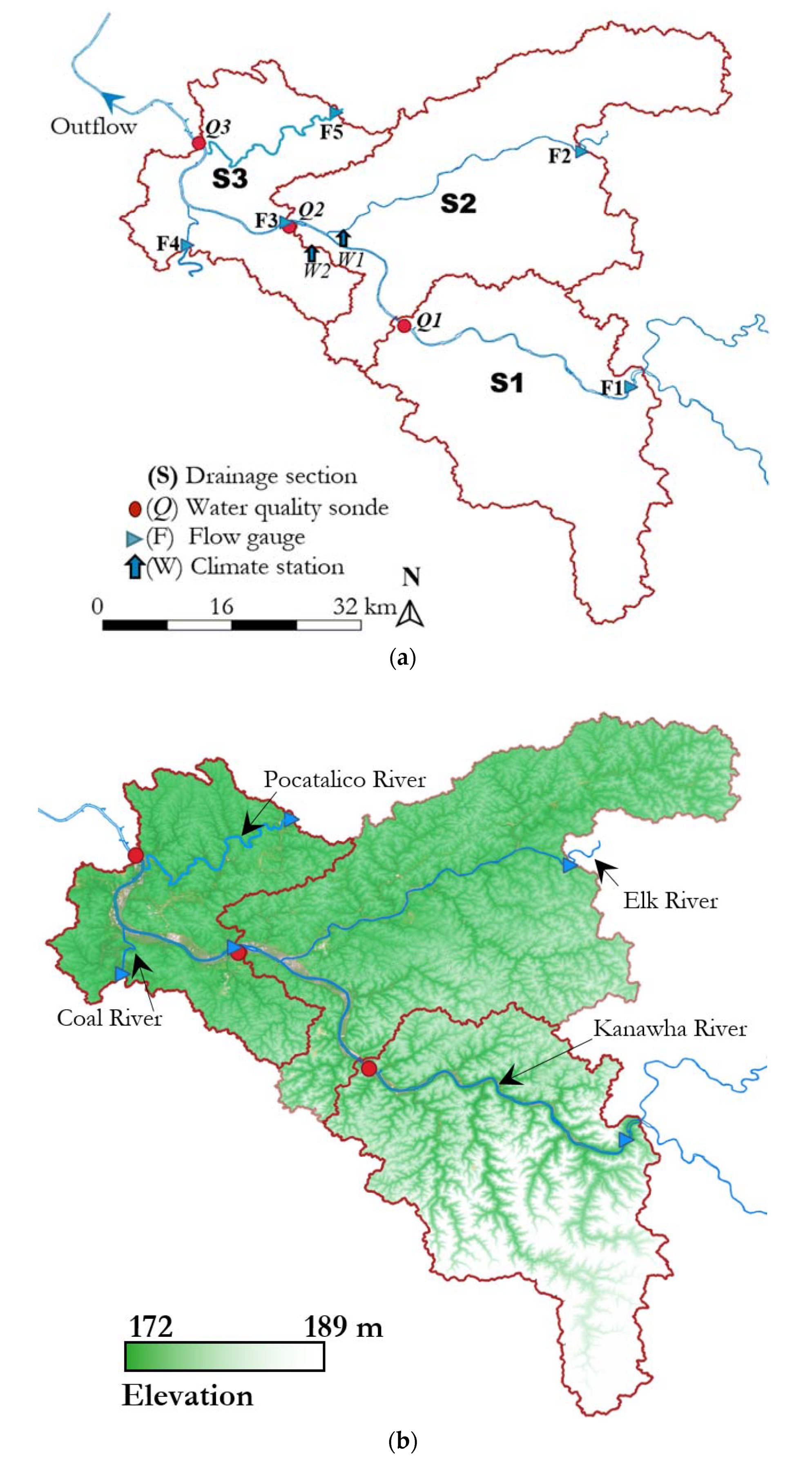
2.1. Watershed Description
2.2. HSPF Model Description
2.3. Multiobjective Calibration of the HSPF Parameters
2.4. Field Measurements of Water Quality
2.5. Net Ecosystem Production
3. Results and Discussion
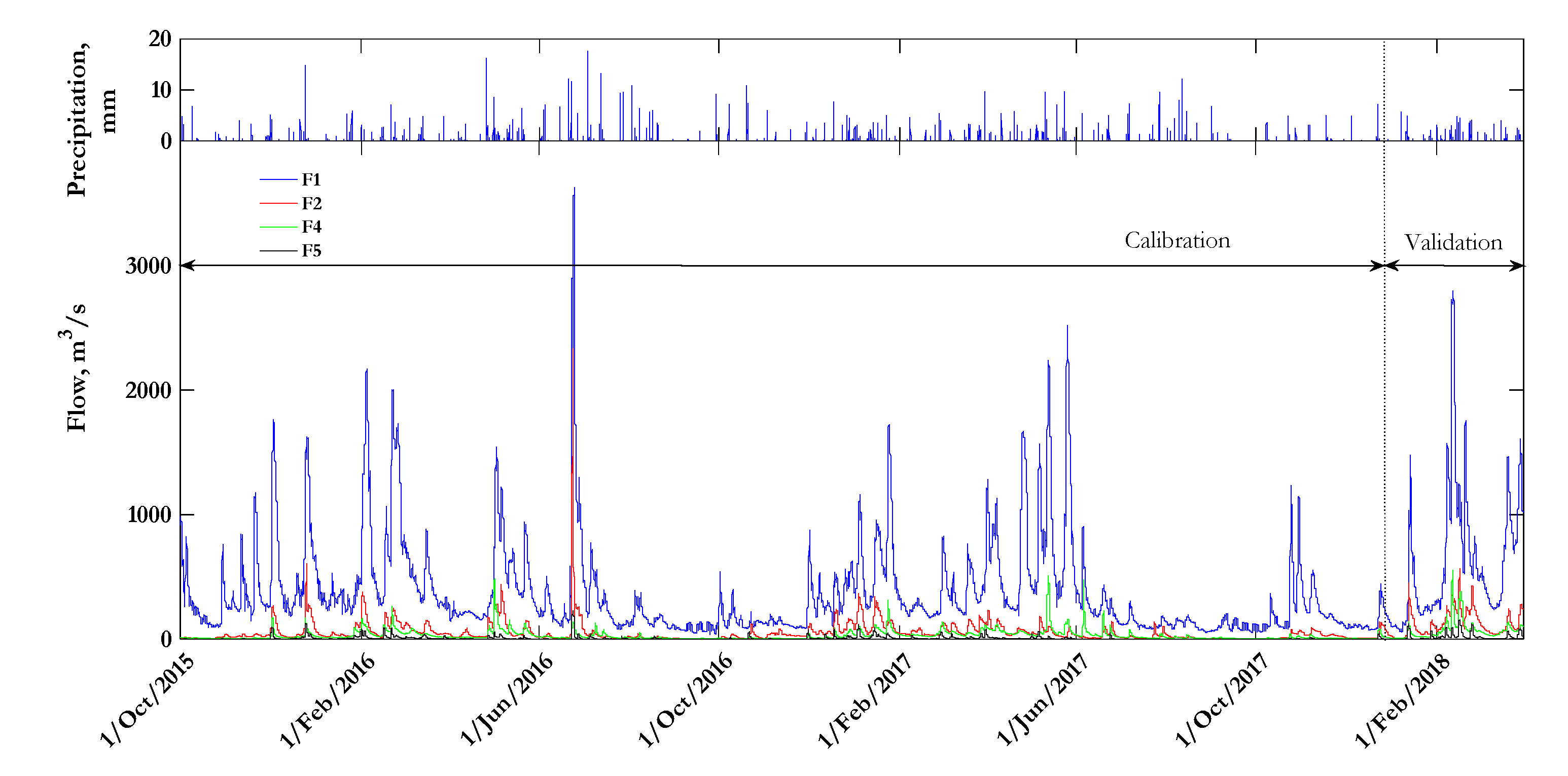
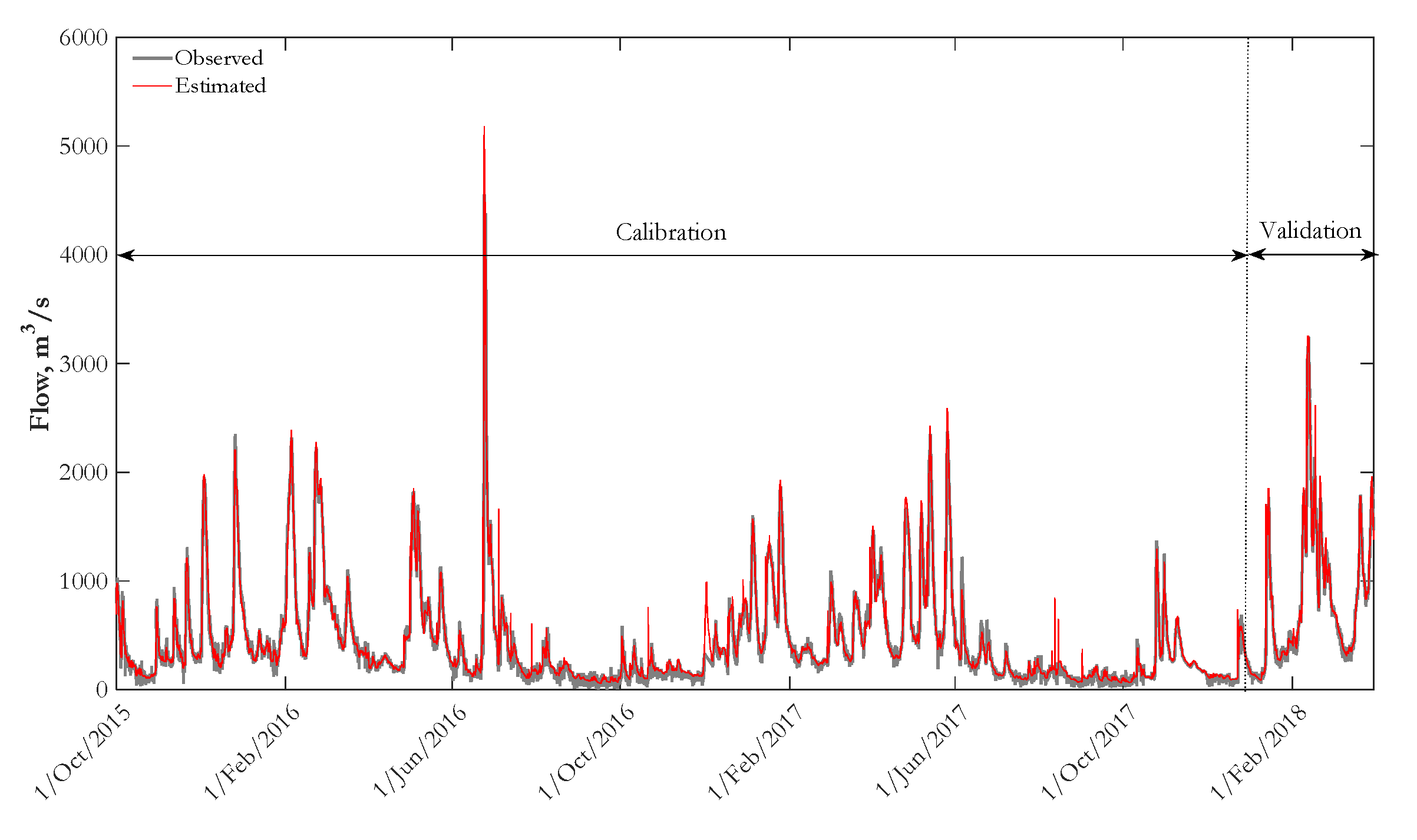
3.1. Input Data and Calibration
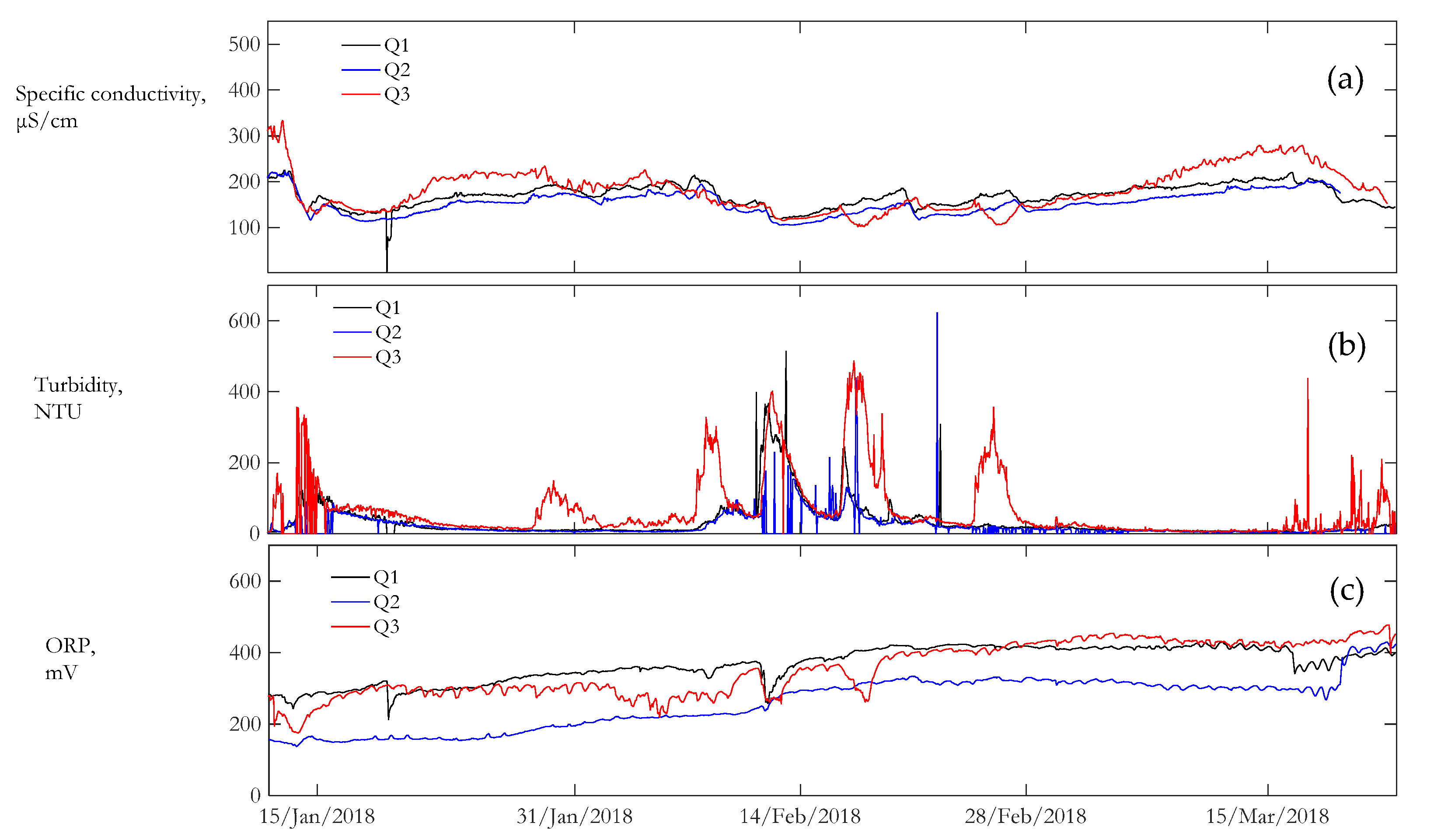
3.2. Water Quality
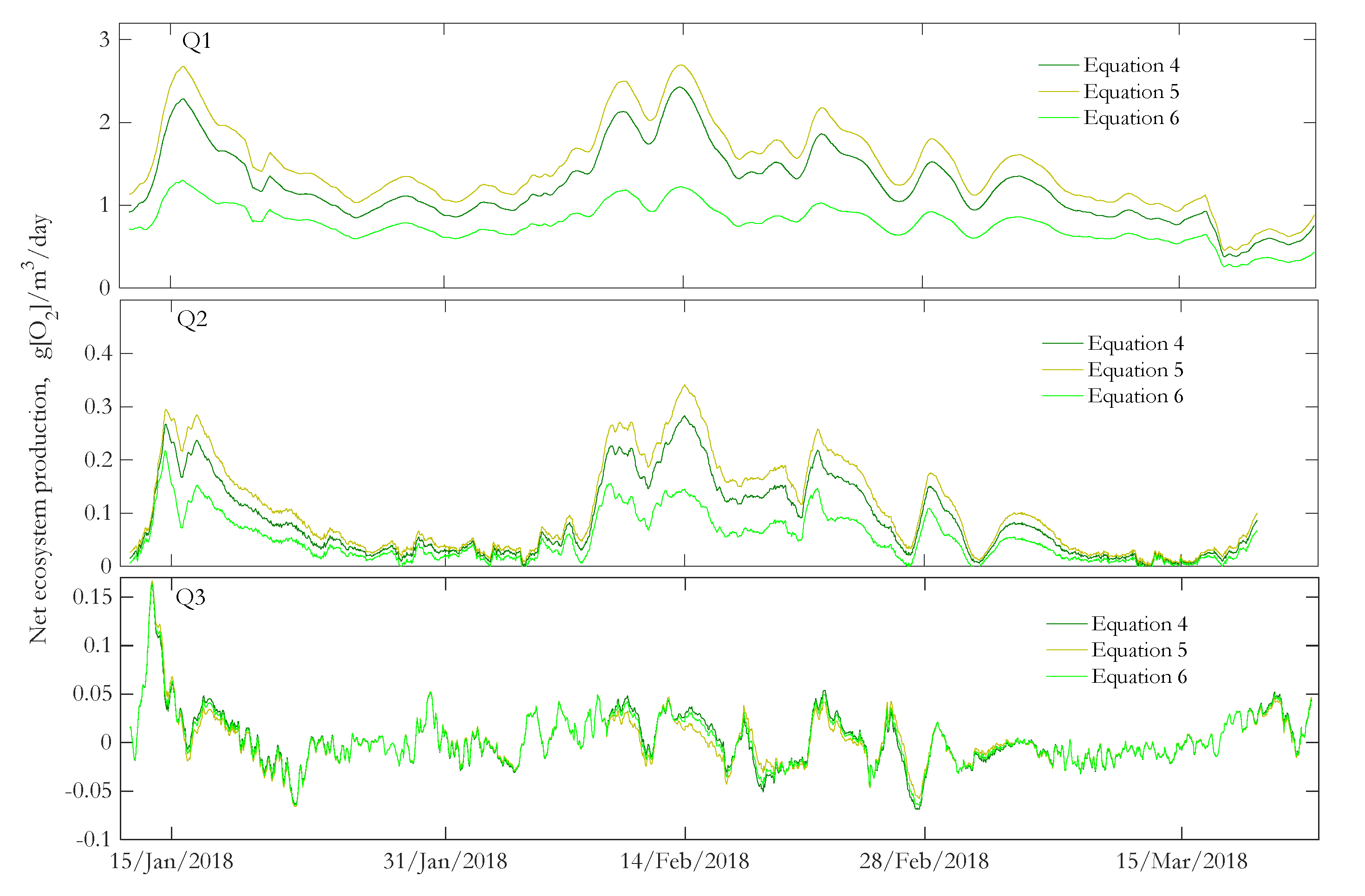
3.3. Net Ecosystem Production
3.4. Spatial and Temporal Variability of NEP
3.5. Impact of Water Quality on NEP and Local Inflows
4. Conclusions
Supplementary Materials
Author Contributions
Funding
Conflicts of Interest
References
- Izagirre, O.; Bermejo, M.; Pozo, J.; Elosegi, A. RIVERMET©: An Excel-based tool to calculate river metabolism from diel oxygen-concentration curves. Environ. Model. Softw. 2007, 22, 24–32. [Google Scholar] [CrossRef]
- Palmer, M.; Ruhi, A. Linkages between flow regime, biota, and ecosystem processes: Implications for river restoration. Science 2019, 365, eaaw2087. [Google Scholar] [CrossRef] [PubMed] [Green Version]
- Uehlinger, U. Annual cycle and inter-annual variability of gross primary production and ecosystem respiration in a floodprone river during a 15-year period. Freshw. Biol. 2006, 51, 938–950. [Google Scholar] [CrossRef]
- Savoy, P.; Appling, A.P.; Heffernan, J.B.; Stets, E.G.; Read, J.S.; Harvey, J.W.; Bernhardt, E.S. Metabolic rhythms in flowing waters: An approach for classifying river productivity regimes. Limnol. Oceanogr. 2019, 64, 1835–1851. [Google Scholar] [CrossRef]
- Odum, H.T. Primary production in flowing waters. Limnol. Oceanogr. 1956, 1, 102–117. [Google Scholar] [CrossRef]
- Staehr, P.A.; Testa, J.M.; Kemp, W.M.; Cole, J.J.; Sand-Jensen, K.; Smith, S.V. The metabolism of aquatic ecosystems: History, applications, and future challenges. Aquat. Sci. 2012, 74, 15–29. [Google Scholar] [CrossRef]
- Staehr, P.A.; Bade, D.; Van de Bogert, M.C.; Koch, G.R.; Williamson, C.; Hanson, P.; Cole, J.J.; Kratz, T. Lake metabolism and the diel oxygen technique: State of the science. Limnol. Oceonogr. Methods 2010, 8, 628–644. [Google Scholar] [CrossRef]
- Lovett, G.M.; Cole, J.J.; Pace, M.L. Is net ecosystem production equal to ecosystem carbon accumulation? Ecosystems 2006, 9, 152–155. [Google Scholar] [CrossRef]
- Hall, R.O.; Tank, J.L.; Baker, M.A.; Rosi-Marshall, E.J.; Hotchkiss, E.R. Metabolism, Gas Exchange, and Carbon Spiraling in Rivers. Ecosystems 2016, 19, 73–86. [Google Scholar] [CrossRef] [Green Version]
- Mejia, F.H.; Fremier, A.K.; Benjamin, J.R.; Bellmore, J.R.; Grimm, A.Z.; Watson, G.A.; Newsom, M. Stream metabolism increases with drainage area and peaks asynchronously across a stream network. Aquat. Sci. 2019, 81, 1–17. [Google Scholar] [CrossRef]
- Beaulieu, J.J.; Arango, C.P.; Balz, D.A.; Shuster, W.D. Continuous monitoring reveals multiple controls on ecosystem metabolism in a suburban stream. Freshw. Biol. 2013, 58, 918–937. [Google Scholar] [CrossRef]
- Blersch, S.S.; Blersch, D.M.; Atkinson, J.F. Metabolic Variance: A Metric to Detect Shifts in Stream Ecosystem Function as a Result of Stream Restoration. J. Am. Water Resour. Assoc. 2019, 55, 608–621. [Google Scholar] [CrossRef]
- Duda, P.B.; Hummel, P.R.; Donigian, A.S., Jr.; Imhoff, J.C. BASINS/HSPF: Model Use, Calibration, and Validation. Trans. ASABE 2012, 55, 1523–1547. [Google Scholar] [CrossRef]
- Chen, W.; He, B.; Nover, D.; Duan, W.; Luo, C.; Zhao, K.; Chen, W. Spatiotemporal patterns and source attribution of nitrogen pollution in a typical headwater agricultural watershed in Southeastern China. Environ. Sci. Pollut. Res. 2018, 25, 2756–2773. [Google Scholar] [CrossRef] [PubMed]
- Fu, B.; Merritt, W.S.; Croke, B.F.W.; Weber, T.R.; Jakeman, A.J. A review of catchment-scale water quality and erosion models and a synthesis of future prospects. Environ. Model. Softw. 2019, 114, 75–97. [Google Scholar] [CrossRef]
- Wagena, M.B.; Collick, A.S.; Ross, A.C.; Najjar, R.G.; Rau, B.; Sommerlot, A.R.; Fuka, D.R.; Kleinman, P.J.A.; Easton, Z.M. Impact of climate change and climate anomalies on hydrologic and biogeochemical processes in an agricultural catchment of the Chesapeake Bay watershed, USA. Sci. Total. Environ. 2018, 637, 1443–1454. [Google Scholar] [CrossRef] [Green Version]
- Deb, K.; Pratap, A.; Agarwal, S.; Meyarivan, T. A fast and elitist multiobjective genetic algorithm: NSGA-II. IEEE Trans. Evol. Comput. 2002, 6, 182–197. [Google Scholar] [CrossRef] [Green Version]
- Panagopoulos, Y.; Makropoulos, C.; Kossida, M.; Mimikou, M. Optimal implementation of irrigation practices: Cost-effective desertification action plan for the Pinios basin. J. Water Resour. Plan. Manag. 2014, 140, 05014005. [Google Scholar] [CrossRef]
- Hassanzadeh, Y.; Afshar, A.A.; Pourreza-Bilondi, M.; Memarian, H.; Besalatpour, A.A. Toward a combined Bayesian frameworks to quantify parameter uncertainty in a large mountainous catchment with high spatial variability. Environ. Monit. Assess. 2019, 191, 1–22. [Google Scholar] [CrossRef]
- Xie, H.; Shen, Z.; Chen, L.; Lai, X.; Qiu, J.; Wei, G.; Dong, J.; Peng, Y.; Chen, X. Parameter estimation and uncertainty analysis: A comparison between continuous and event-based modeling of streamflow based on the Hydrological Simulation Program-Fortran (HSPF) model. Water 2019, 11, 171. [Google Scholar] [CrossRef] [Green Version]
- Zhang, R.; Moreira, M.; Corte-Real, J. Multi-objective calibration of the physically based, spatially distributed SHETRAN hydrological model. J. Hydroinform. 2015, 18, 428–445. [Google Scholar] [CrossRef] [Green Version]
- Dumedah, G.; Berg, A.A.; Wineberg, M.; Collier, R. Selecting Model Parameter Sets from a Trade-off Surface Generated from the Non-Dominated Sorting Genetic Algorithm-II. Water Resour. Manag. 2010, 24, 4469–4489. [Google Scholar] [CrossRef]
- Mostafaie, A.; Forootan, E.; Safari, A.; Schumacher, M. Comparing multi-objective optimization techniques to calibrate a conceptual hydrological model using in situ runoff and daily GRACE data. Comput. Geosci. 2018, 22, 789–814. [Google Scholar] [CrossRef] [Green Version]
- Lampert, D.J.; Wu, M. Development of an open-source software package for watershed modeling with the Hydrological Simulation Program in Fortran. Environ. Model. Softw. 2015, 68, 166–174. [Google Scholar] [CrossRef] [Green Version]
- Raymond, P.A.; Zappa, C.J.; Butman, D.; Bott, T.L.; Potter, J.; Mulholland, P.; Laursen, A.E.; McDowell, W.H.; Newbold, D. Scaling the gas transfer velocity and hydraulic geometry in streams and small rivers. Limnol. Oceanogr. Fluids Environ. 2012, 2, 41–53. [Google Scholar] [CrossRef]
- Hall, R.O.; Ulseth, A.J. Gas Exchange in Streams and Rivers. WIREs Water 2019, 1–18. [Google Scholar] [CrossRef]
- Zappa, C.J.; McGillis, W.R.; Raymond, P.A.; Edson, J.B.; Hintsa, E.J.; Zemmelink, H.J.; Dacey, J.W.H.; Ho, D.T. Environmental turbulent mixing controls on air-water gas exchange in marine and aquatic systems. Geophys. Res. Lett. 2007, 34, 1–6. [Google Scholar] [CrossRef] [Green Version]
- Wanninkhof, R. Relationship between wind speed and gas exchange over the ocean revisited. Limnol. Oceanogr. Methods 2014, 12, 351–362. [Google Scholar] [CrossRef]
- Hill, N.B.; Riha, S.J.; Walter, M.T. Temperature dependence of daily respiration and reaeration rates during baseflow conditions in a northeastern U.S. stream. J. Hydrol. Reg. Stud. 2018, 19, 250–264. [Google Scholar] [CrossRef]
- Engel, F.; Attermeyer, K.; Ayala, A.I.; Fischer, H.; Kirchesch, V.; Pierson, D.C.; Weyhenmeyer, G.A. Phytoplankton gross primary production increases along cascading impoundments in a temperate, low-discharge river: Insights from high frequency water quality monitoring. Sci. Rep. 2019, 9, 1–13. [Google Scholar] [CrossRef]
- Bernhardt, E.S.; Heffernan, J.B.; Grimm, N.B.; Stanley, E.H.; Harvey, J.W.; Arroita, M.; Appling, A.P.; Cohen, M.J.; McDowell, W.H.; Hall, R.O.; et al. The metabolic regimes of flowing waters. Limnol. Oceanogr. 2018, 63, S99–S118. [Google Scholar] [CrossRef] [Green Version]
- Demars, B.O.L.; Thompson, J.; Manson, J.R. Stream metabolism and the open diel oxygen method: Principles, practice, and perspectives. Limnol. Oceanogr. Methods 2015, 13, 356–374. [Google Scholar] [CrossRef] [Green Version]
- Mansoor, S.Z.; Louie, S.; Lima, A.T.; Van Cappellen, P.; MacVicar, B. The spatial and temporal distribution of metals in an urban stream: A case study of the Don River in Toronto, Canada. J. Great Lakes Res. 2018, 44, 1314–1326. [Google Scholar] [CrossRef]
- Abdul-Aziz, O.I.; Ahmed, S. Relative linkages of stream water quality and environmental health with the land use and hydrologic drivers in the coastal-urban watersheds of southeast Florida. GeoHealth 2017, 1, 180–195. [Google Scholar] [CrossRef] [Green Version]
- Fuß, T.; Behounek, B.; Ulseth, A.J.; Singer, G.A. Land use controls stream ecosystem metabolism by shifting dissolved organic matter and nutrient regimes. Freshw. Biol. 2017, 62, 582–599. [Google Scholar] [CrossRef]
- O’Brien, J.M.; Warburton, H.J.; Elizabeth Graham, S.; Franklin, H.M.; Febria, C.M.; Hogsden, K.L.; Harding, J.S.; McIntosh, A.R. Leaf litter additions enhance stream metabolism, denitrification, and restoration prospects for agricultural catchments. Ecosphere 2017, 8, 1–17. [Google Scholar] [CrossRef]
- Griffiths, N.A.; Tank, J.L.; Royer, T.V.; Roley, S.S.; Rosi-Marshall, E.J.; Whiles, M.R.; Beaulieu, J.J.; Johnson, L.T. Agricultural land use alters the seasonality and magnitude of stream metabolism. Limnol. Oceanogr. 2013, 58, 1513–1529. [Google Scholar] [CrossRef]
- National Solar Radiation Database. Available online: https://nsrdb.nrel.gov (accessed on 27 May 2019).
- Berndt, M.E.; Rutelonis, W.; Regan, C.P. A comparison of results from a hydrologic transport model (HSPF) with distributions of sulfate and mercury in a mine-impacted watershed in northeastern Minnesota. J. Environ. Manag. 2016, 181, 74–79. [Google Scholar] [CrossRef] [Green Version]
- Bello, A.A.D.; Haniffah, M.R.M.; Hanapi, M.N.; Usman, A.B. Identification of critical source areas under present and projected land use for effective management of diffuse pollutants in an urbanized watershed. Int. J. River Basin Manag. 2019, 17, 171–184. [Google Scholar] [CrossRef]
- Borah, D.K.; Bera, M. Watershed-Scale Hydrologic and Nonpoint-Source Pollution Models: Review of Applications. Trans. ASAE 2013, 47, 789–803. [Google Scholar] [CrossRef] [Green Version]
- Nash, J.E.; Sutcliffe, J.V. River flow forecasting through conceptual models part I—A discussion of principles. J. Hydrol. 1970, 10, 282–290. [Google Scholar] [CrossRef]
- Moriasi, D.N.; Arnold, J.G.; Van Liew, M.W.; Bingner, R.L.; Harmel, R.D.; Veith, T.L. Model evaluation guidelines for systematic quantification of accuracy in watershed simulations. Am. Soc. Agric. Biol. Eng. 2007, 50, 885–900. [Google Scholar]
- Pandey, P.K.; Dabral, P.P.; Pandey, V. Evaluation of reference evapotranspiration methods for the northeastern region of India. Int. Soil Water Conserv. Res. 2016, 4, 52–63. [Google Scholar] [CrossRef] [Green Version]
- Huber, D.H.; Ugwuanyi, I.R.; Lhilhi, N.V.; Kemajou, T.; Andrielle, L.; Chavarria-Palma, J.E. Water Quality for Kanawha River WV. Available online: https://doi.org/10.6084/m9.figshare.9786212.v1 (accessed on 22 September 2019).
- Appling, A.P.; Hall, R.O.; Yackulic, C.B.; Arroita, M. Overcoming Equifinality: Leveraging Long Time Series for Stream Metabolism Estimation. J. Geophys. Res. Biogeosci. 2018, 123, 624–645. [Google Scholar] [CrossRef] [Green Version]
- Tang, G.; Zhu, Y.; Wu, G.; Li, J.; Li, Z.L.; Sun, J. Modelling and analysis of hydrodynamics and water quality for rivers in the northern cold Region of China. Int. J. Environ. Res. Public Health 2016, 13, 408. [Google Scholar] [CrossRef] [Green Version]
- Falkowski, T.; Ostrowski, P.; Siwicki, P.; Brach, M. Channel morphology changes and their relationship to valley bottom geology and human interventions; a case study from the Vistula Valley in Warsaw, Poland. Geomorphology 2017, 297, 100–111. [Google Scholar] [CrossRef]
- Read, J.S.; Hamilton, D.P.; Desai, A.R.; Rose, K.C.; MacIntyre, S.; Lenters, J.D.; Smyth, R.L.; Hanson, P.C.; Cole, J.J.; Staehr, P.A.; et al. Lake-size dependency of wind shear and convection as controls on gas exchange. Geophys. Res. Lett. 2012, 39, 1–5. [Google Scholar] [CrossRef] [Green Version]
- Halbedel, S.; Büttner, O.; Weitere, M. Linkage between the temporal and spatial variability of dissolved organic matter and whole-stream metabolism. Biogeosciences 2013, 10, 5555–5569. [Google Scholar] [CrossRef] [Green Version]
- Demars, B.O.L.; Russell, M.J.; Ólafsson, J.S.; Gíslason, G.M.; Gudmundsdóttir, R.; Woodward, G.; Reiss, J.; Pichler, D.E.; Rasmussen, J.J.; Friberg, N. Temperature and the metabolic balance of streams. Freshw. Biol. 2011, 56, 1106–1121. [Google Scholar] [CrossRef]
- Reichert, P.; Uehlinger, U.; Acuña, V. Estimating stream metabolism from oxygen concentrations: Effect of spatial heterogeneity. J. Geophys. Res. Biogeosci. 2009, 114, 1–15. [Google Scholar] [CrossRef] [Green Version]
- Huber, D.H.; Ugwuanyi, I.R.; Malkaram, S.A.; Montenegro-Garcia, N.A.; Lhilhi, N.V.; Chavarria-Palma, J.E. Metagenome Sequences of Sediment from a Recovering Industrialized Appalachian River in West Virginia. Genome Announc. 2018, 6, e00350-18. [Google Scholar] [CrossRef] [PubMed] [Green Version]
- Bernot, M.J.; Sobota, D.J.; Hall, R.O.; Mulholland, P.J.; Dodds, W.K.; Webster, J.R.; Tank, J.L.; Ashkenas, L.R.; Cooper, L.W.; Dahm, C.N.; et al. Inter-regional comparison of land-use effects on stream metabolism. Freshw. Biol. 2010, 55, 1874–1890. [Google Scholar] [CrossRef]
- Uehlinger, U.; Kawecka, B.; Robinson, C.T. Effects of experimental floods on periphyton and stream metabolism below a high dam in the Swiss Alps (River Spöl). Aquat. Sci. 2003, 65, 199–209. [Google Scholar] [CrossRef] [Green Version]
- Izagirre, O.; Agirre, U.; Bermejo, M.; Pozo, J.; Elosegi, A. Environmental controls of whole-stream metabolism identified from continuous monitoring of Basque streams. J. N. Am. Benthol. Soc. 2008, 27, 252–268. [Google Scholar] [CrossRef]
- Sánchez-Pérez, J.M.; Gerino, M.; Sauvage, S.; Dumas, P.; Maneux, É.; Julien, F.; Winterton, P.; Vervier, P. Effects of wastewater Treatment Plant pollution on in-stream ecosystems functions in an agricultural watershed. Ann. Limnol. 2009, 45, 79–92. [Google Scholar] [CrossRef] [Green Version]
- Kaushal, S.S.; Delaney-Newcomb, K.; Findlay, S.E.G.; Newcomer, T.A.; Duan, S.; Pennino, M.J.; Sivirichi, G.M.; Sides-Raley, A.M.; Walbridge, M.R.; Belt, K.T. Longitudinal patterns in carbon and nitrogen fluxes and stream metabolism along an urban watershed continuum. Biogeochemistry 2014, 121, 23–44. [Google Scholar] [CrossRef]
- Grace, M.R.; Giling, D.P.; Hladyz, S.; Caron, V.; Thompson, R.M.; Mac Nally, R. Fast processing of diel oxygen curves: Estimating stream metabolism with base (BAyesian single-station estimation). Limnol. Oceanogr. Methods 2015, 13, 103–114. [Google Scholar] [CrossRef]
- Tang, S.; Sun, T.; Shen, X.M.; Qi, M.; Feng, M.L. Modeling net ecosystem metabolism influenced by artificial hydrological regulation: AN application to the Yellow River Estuary, China. Ecol. Eng. 2015, 76, 84–94. [Google Scholar] [CrossRef]


| Latitude (N) | Longitude (W) | Elevation (m) | ||
|---|---|---|---|---|
| Flow gage | F1 | 38.1381° | 81.2144° | 190 |
| F2 | 38.4714° | 81.2839° | 186 | |
| F3 | 38.3714° | 81.7022° | 173 | |
| F4 | 38.3389° | 81.8412° | 177 | |
| F5 | 38.5261° | 81.6310° | 183 | |
| Weather stations | W1 | 38.3794° | 81.5900° | 279 |
| W2 | 38.3131° | 81.7192° | 277 | |
| Water quality sondes | Q1 | 38.2244° | 81.5356° | 181 |
| Q2a | 38.3638° | 81.6630° | 173 | |
| Q2b | 38.3625° | 81.6642° | 173 | |
| Q2c | 38.3625° | 81.6642° | 170.5 | |
| Q3 | 38.4828° | 81.8258° | 172 |
| S1 (km2) | S2 (km2) | S3 (km2) | ||
|---|---|---|---|---|
| Land Use | Urban | 33.33 | 88.32 | 49.1 |
| Agriculture | 14.68 | 39.6 | 36.34 | |
| Forest | 899.7 | 1307 | 359.83 | |
| Wetland | 9.5 | 7.69 | 5.18 | |
| Barren | 131.75 | 11.11 | 1.71 | |
| Drainage Section | Stream | Length, km | Elevation Change, m | Average Slope, m | Average Width, m |
|---|---|---|---|---|---|
| 1 | Kanawha River | 38.5 | 9 * | 0.00005 | 183 |
| 2 | Kanawha River | 23.5 | 7.8 * | 0.00004 | 183 |
| Elk River | 41.5 | 13 | 0.00031 | 76 | |
| 3 | Kanawha River | 29.3 | 0.61 | 0.00003 | 183 |
| Coal River | 18.7 | 4.57 | 0.00024 | 52 | |
| Pocatalico River | 41 | 10.4 | 0.00025 | 31 |
| Parameter | Units | Meaning | Range or Averaged Data |
|---|---|---|---|
| LZSN | (mm) | Lower zone nominal storage | 51–381 |
| INFILT | (mm/h) | Index to soil infiltration capacity | 0.02–13 |
| LSUR | (m) | Average length of the assumed overland flow plane | 69.2 * |
| SLSUR | (-) | Average slope of the overland flow plane | 0.107 * |
| KVARY | (1/mm) | Variable groundwater recession flow | 0–0.2 |
| AGWRC | (1/day) | Basic groundwater recession rate | 0.85–0.99 |
| PETMAX | (°C) | Air temperature below which evapotranspiration (ET) will arbitrarily be reduced below the value obtained from the input time series | 4.4 * |
| PETMIN | (°C) | Temperature below which E-T will be zero regardless of the value in the input time series | 1.7 * |
| INFEXP | (-) | Exponent in the infiltration equation | 2 ** |
| DEEPFR | (-) | Fraction of groundwater inflow which will enter deep (inactive) groundwater | 0–0.5 |
| BASETP | (-) | Base flow evapotranspiration | 0–0.2 |
| AGWETP | (-) | Fraction of remaining potential E-T which can be satisfied from active groundwater storage | 0–0.2 |
| CEPSC | (mm) | Interception storage capacity | 0–10 |
| UZSN | (mm) | Upper zone nominal storage | 1–51 |
| NSUR | (-) | Manning’s n for overland flow | 0.1–0.5 |
| INTFW | (-) | Interflow inflow parameter | 1–10 |
| IRC | (1/day) | Interflow recession constant | 0.3–0.85 |
| LZETP | (-) | Lower zone E-T parameter. It is an index to the density of deep-rooted vegetation. | 0–0.9 |
| LAT | (°) | Latitude of the pervious land segment (PLS) | 38 * |
| MELEV | (m) | Mean elevation of the PLS | 181 * |
| Precipitation, mm | Temperature, °C | Dew Point Temperature 1, °C | Evapotranspiration (EVT), mm | ||||||
|---|---|---|---|---|---|---|---|---|---|
| Source | Station | NLDAS | Station | NLDAS | Station | NLDAS and AIRS | Station | NLDAS | Potential EVT |
| Mean | 2.54 | 2.91 | 12.78 | 12.88 | 7.72 | 10.11 | 0.965 | 1.677 | 4.318 |
| CV | 2.292 | 2.085 | 0.299 | 0.302 | 0.380 | 0.368 | 0.964 | 0.706 | 0.533 |
| Parameter | Value | Parameter | Value |
|---|---|---|---|
| LZSN | 51 | CEPSC | 9.7 |
| INFILT | 6.1 | UZSN | 4.4 |
| KVARY | 0.098 | NSUR | 0.109 |
| AGWRC | 0.98 | INTFW | 2.647 |
| DEEPFR | 0.494 | IRC | 0.302 |
| BASETP | 0.198 | LZETP | 0.709 |
| AGWETP | 0.105 |
| Measure | HSPEXP Limit | |
|---|---|---|
| Error in total volume, % | 1.71 | 10 |
| Error of highest 10% flows, % | −0.21 | 15 |
| Error of highest 25% flows, % | −0.49 | 10 |
| Error of highest 50% flows, % | −0.03 | 10 |
| Error of lowest 50% flows, % | 9.59 | 10 |
| Error of lowest 25% flows, % | 13.29 | 15 |
| Error of lowest 10% flows, % | 14.72 | 20 |
| Location | Temperature | Dissolved Oxygen | Dissolved Oxygen Saturation | Specific Conductance | Turbidity | ORP |
|---|---|---|---|---|---|---|
| Q1 | 0.551 | 0.097 | 0.042 | 0.142 | 1.549 | 0.134 |
| Q2 | 0.543 | 0.192 | 0.029 | 0.280 | 1.628 | 0.281 |
| Q3 | 0.529 | 0.304 | 0.030 | 0.266 | 1.311 | 0.208 |
| Location | Repetition | N | Depth, m | Velocity, m/s | Water Temperature, °C | Dissolved Oxygen, mg/L | NEP, g[O2]/m3/day |
|---|---|---|---|---|---|---|---|
| Q2a | 1 | 36 | 1 | 0.12 | 28.3 (±0.9) | 8.6 (±0.3) | 4.3 |
| 2 | 54 | 1 | 0.08 | 26.7 (±1.2) | 9.2 (±0.5) | 3.3 | |
| 3 | 163 | 1 | 0.05 | 26 (±0.5) | 8.3 (±0.1) | 1.7 | |
| Q2b | 1 | 63 | 1 | 0.11 | 27.8 (±0.8) | 8.2 (±0.2) | 1.8 |
| 2 | 49 | 1 | 0.08 | 26 (±0.5) | 8.2 (±0.1) | 0.9 | |
| 3 | 73 | 1 | 0.05 | 27.3 (±1.7) | 8.7 (±0.3) | 1.2 | |
| Q2c | 1 | 62 | 2.5 | 0.06 | 26.7 (±1.5) | 8.4 (±0.3) | 0.8 |
| 2 | 60 | 2.5 | 0.04 | 26.3 (±1.0) | 8.4 (±0.1) | 0.7 | |
| 3 | 70 | 2.5 | 0.05 | 26.6 (±1.3) | 8.4 (±0.2) | 0.9 |
| Location | N | Velocity, m/s | Water Temperature, °C | Dissolved Oxygen, mg/L | NEP, g[O2]/m3/day |
|---|---|---|---|---|---|
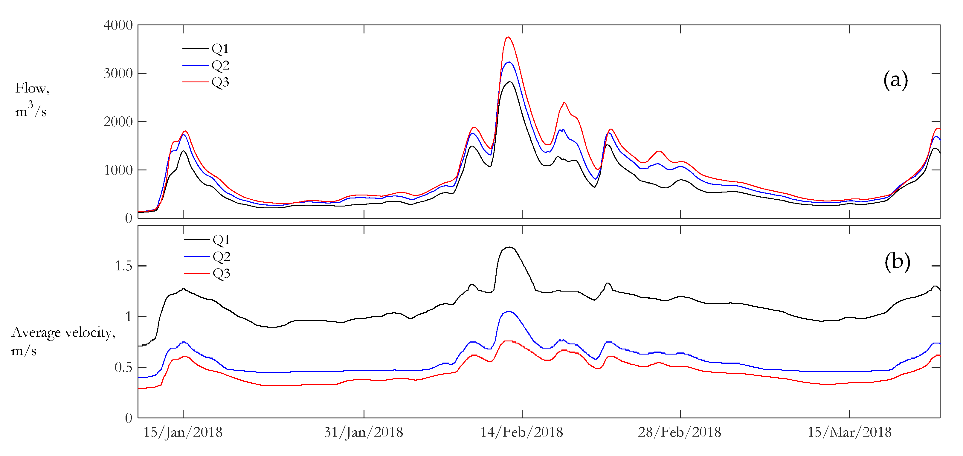
| Q1 | 1682 | 1.11 (±0.16) | 5.5 (±3) | 14.9 (±1.4) | 1.24 (±0.4) |
| Q2 | 1600 | 0.6 (±0.13) | 5.4 (±3) | 6.1 (±1.2) | 0.09 (±0.07) |
| Q3 | 1674 | 0.46 (±0.11) | 5.4 (±3) | 4.8 (±1.5) | 0.004 (±0.03) |
| Specific Conductance | Turbidity | |
|---|---|---|
| NEPQ1 | −0.61 | 0.81 |
| NEPQ2 | −0.57 | 0.41 |
| NEPQ3 | −0.01 | 0.06 |
| Local Inflows | NEP | Specific Conductance | Turbidity | ORP |
|---|---|---|---|---|
| WQ1–Q2 | −0.71 | −0.28 | −0.55 | 0.42 |
| WQ2–Q3 | −0.42 | −0.61 | 0.15 | −0.29 |
© 2020 by the authors. Licensee MDPI, Basel, Switzerland. This article is an open access article distributed under the terms and conditions of the Creative Commons Attribution (CC BY) license (http://creativecommons.org/licenses/by/4.0/).
Share and Cite
Rojano, F.; Huber, D.H.; Ugwuanyi, I.R.; Noundou, V.L.; Kemajou-Tchamba, A.L.; Chavarria-Palma, J.E. Net Ecosystem Production of a River Relying on Hydrology, Hydrodynamics and Water Quality Monitoring Stations. Water 2020, 12, 783. https://doi.org/10.3390/w12030783
Rojano F, Huber DH, Ugwuanyi IR, Noundou VL, Kemajou-Tchamba AL, Chavarria-Palma JE. Net Ecosystem Production of a River Relying on Hydrology, Hydrodynamics and Water Quality Monitoring Stations. Water. 2020; 12(3):783. https://doi.org/10.3390/w12030783
Chicago/Turabian StyleRojano, Fernando, David H Huber, Ifeoma R Ugwuanyi, Vadesse Lhilhi Noundou, Andrielle Larissa Kemajou-Tchamba, and Jesus E Chavarria-Palma. 2020. "Net Ecosystem Production of a River Relying on Hydrology, Hydrodynamics and Water Quality Monitoring Stations" Water 12, no. 3: 783. https://doi.org/10.3390/w12030783