A Cusp Catastrophe Model for Alluvial Channel Pattern and Stability

Abstract

The self-adjustment of an alluvial channel is a complicated process with various factors influencing the stability and transformation of channel patterns. A cusp catastrophe model for the alluvial channel regime is established by selecting suitable parameters to quantify the channel pattern and stability. The channel patterns can be identified by such a model in a direct way with a quantified index, which is a 2D projection of the cusp catastrophe surface, and the discriminant function is obtained from the model to distinguish the river state. Predictions based on this model are consistent with the field observations involving about 150 natural rivers of small or medium sizes. This new approach enables us to classify the channel pattern and determine a river stability state, and it paves the way toward a better understanding of the regime of natural rivers to assist decision-making in river management.

1. Introduction

The self-adjustment of an alluvial channel is a complicated process with various factors influencing the stability and transformation of channel patterns. Although the formation of alluvial channels has been extensively studied, the problem of the alluvial channel stability still remains to be systematically resolved. Analysis of channel stability entails the determination of how a channel adjusts its river geometry in response to the water and sediment influxes imposed by its watershed [1]. The most important parameters for determining channel stability are its top width, average flow depth, flow velocity, and longitudinal slope. Therefore, efforts to understand the sustainability concept and present hydraulic geometry relations have been made. Several previous works have obtained a series of relationships for predicting a stable channel. In general, there are three approaches to determine the channel status: (1) empirical relationships and the regime method [2,3]; (2) the mechanical method of tensile force [4,5]; and (3) extremal or limiting methods [6,7,8]. The main difference between these theories is in the hydraulic mechanisms used to explain how flow balance can be achieved. In fact, the fundamentals of the regime theory lie in statistical methods with large numbers of observations. However, the basic assumption in all theories is constant and uniform flow intended to achieve equilibrium and semi-equilibrium balance.

The identification of geomorphic and hydrologic thresholds that determine alluvial channel patterns (e.g., braided, meandering, and straight) has long been an important research focus in fluvial systems; it is now well known that alluvial channel patterns are influenced by at least seven primary controlling variables: channel slope, discharge, valley confinement, sediment supply, grain diameter, bank strength, and wood loading [9,10]. While the role of each of these variables is generally understood, this fundamental link between form and process has provided the theoretical basis upon which numerous river classification schemes have been developed [11,12,13,14]. However, there are just a few attempts to incorporate these variables into a predictive model of channel pattern [10]; some researchers statistically analyzed large and complex geospatial data sets and developed predictive models of channel patterns [10,15,16]. The diversity of these methods and the selection criteria for one or another is influenced by different reasons, for example, objectives and scale of work (site, network, and watershed), time requirements and data, statistical and programmer expertise, or the complexity of the area of study and its analysis and interpretation.

Catastrophe theory is a mathematical method for describing system behavior where a gradually changing force can produce a sudden dramatic effect. Rene Thom published the first paper on it in 1968, and then the first book in 1972 [17], and now it has found applications in a wide variety of disciplines, including physics, biology, psychology, economics, and geology [18,19,20,21,22]. With the development of nonlinear mathematics, some researchers have adopted catastrophe theory to describe the changes in river morphology. Thornes studied the characteristics of Spanish rivers based on the nonlinear mathematics theory [23]; Richards brought catastrophe theory into the mechanism of fluvial processes to discuss the variables in the transition [24]; Graf described the transformation among straight, meandering and braided river with the cusp catastrophe theory, and pointed out that rivers may result in different patterns although under the same sediment-discharge and boundary conditions [25]. The research results illustrate the effectiveness of the stability analysis of river patterns using catastrophe theory. Nevertheless, the catastrophe theory only explains the phenomenon for channel stability and their transition and lackeds quantitative results.

This paper aims to propose an equilibrium equation of channel regime to investigate channel stability and then establish a function to distinguish the alluvial channel patterns, based on the cusp catastrophe model. The model enables the discrimination and the prediction of the equilibrium state for channel patterns based on the appropriate control and state variables. One hundred fifty natural rivers are used to test the reliability of the model, and then the model is applied in the river reach in the upstream reaches of the Yangtze River to investigate the temporal change of channel pattern and its statue. The results indicate that this approach can be used to judge river patterns and states when the control factors can be obtained in the field, to study the regime of natural rivers, and to give some suggestions to river management.

2. The Cusp Catastrophe Model for Channel Regime

2.1. The Cusp Catastrophe Model

Behaviors of dynamical systems can usually be described by differential equations called entropy function. In applying science, it is customary to divide it into two groups: first, the space is of finite dimension (LPS), and second, it is of infinite dimension (DPS). In this paper, we adopt the first type, called lumped-parameter systems (LPS). The phase’s space of LPS is a finite-dimensional space, which is defined as an n-dimensional Euclidean space. The LPS can be usually written in the form:

$$dS=\frac{d{z}_i}{dt}=f(z_1,z_2\cdots z_n,{\alpha }_1,{\alpha }_2\cdots {\alpha }_m), i=1,2\cdots n$$

(1)

where z_i denotes the state variable, t is time, and α_i is generally a system parameter.

In this study, there are two assumptions for the dynamical system: one is autonomous to make sure the time variable does not occur on the right-hand sides (RHS) explicitly, and the other is continuous by using the continuously differentiable functions for their arguments. The steady-state (stationary) solution z of the system satisfies the nonlinear equation as follows:

$$f(z_1,z_2\cdots z_n,{\alpha }_1,{\alpha }_2\cdots z_m)=0, i=1,2\cdots n$$

(2)

There are many types of approaches to investigating dynamic systems. The most general, qualitative, and topological techniques are used to classify topologically distinct types of behavior possible in the given model. Catastrophe theory belongs to this category. It was created by Rene Thom [17]. The theory is based on new theorems in multi-dimensional geometry, which classify the way that the discontinuities can occur in terms of a few archetypal forms.

Of the seven elementary catastrophes in catastrophe theory, the cusp model is the most widely applied. It is often used to model the behavior of a system with two control parameters and a non-linear state parameter. The potential function E for the cusp catastrophe is [26]

$$E=\frac{1}{4}{z}^4+\frac{1}{2}x{z}^2-yz$$

(3)

Its equilibrium points, as a function of the control parameters x and y are solutions to the equation as follows:

$$\frac{dE}{dz}=f(x,y,z)=z^3+xz-y=0$$

(4)

where $x,y$ are defined as the control parameters; z is the state parameter of the system.

Based on the similarity between the entropy function of dissipative structures and the potential function in the catastrophe theory, it can be described as the steady-state equation to express the state of a system with the cusp catastrophe model:

$$dS=\frac{dE}{dz}$$

(5)

Cardan’s discriminant can be used to describe the state of the dynamic system, which is written as

$$\Delta =4x^3+27y^3$$

(6)

where Equation (6) has one solution if △ > 0, and has three solutions if △ < 0. The set of values of x and y for which △ = 0 demarcates the bifurcation set. These solutions are depicted as a two-dimensional surface in a three-dimensional space, the floor of which is the two-dimensional (x, y) coordinates system called the "control plane".

2.2. Determination of the Control Parameters and the State Parameter

The morphology of natural river channels is determined by the interaction of fluid flow with the erodible materials in the channel boundary [27]. The interrelationships between the (1) oncoming bed material load and the sediment carrying capacity of the flow, and (2) the erodibility of the river banks and the erosive power of the water decide essentially the general direction of the self-adjustment. Besides a variety of available methods for predicting channel stability parameters, a point of high research interest is the effect of hydraulic parameters and factors, such as the discharge, median grain size, Shields parameter, vegetation type, average roughness, and sediment composition [28,29,30,31,32]. On the basis of the preliminary analysis of the multitude of parameters reported in the literature, the synthetic indexes of river-bed stability determined by the longitudinal river-bed stability in contrast to the transverse river-bed stability are adopted in this study, the longitudinal index of B.и.AcrpaxaниeB, and the transverse index of C. T. Aлтунин are expressed in the form [27]:

$${\varphi }_b=\frac{B}{B_1}=\frac{B{J}^{0.2}}{Q^{0.5}}$$

(7)

$${\varphi }_h=\frac{({\gamma }_s-\gamma )D_{50}}{\gamma hJ}$$

(8)

where ϕ_h is the longitudinal index, and ϕ_b is the transverse index; h, J are defined as the local water depth and channel slope; Q denotes the bank-full discharge; B is the channel width under the bank-full discharge; D₅₀ is the median bed material grain size; γ,γ_s is the volumetric weight of the water and sediment, respectively.

The transverse index can reflect the channel planform changes; we decide ϕ₁ as the dominant control parameter and ϕ₂ as the second control parameter that determines the channel scouring and deposition. The control parameters can be written as:

$${\varphi }_1={({\varphi }_b)}^a$$

(9)

$${\varphi }_2={\left({\varphi }_h\right)}^b$$

(10)

where a, b are the weight coefficients, satisfied with a + b = 1. Considering the importance of the oncoming bed material and the erodibility in the river process, we assumed a = b = 1/2 when a + b = 1.

The state parameter is often used to describe the behavior of a system, which is influenced by the control parameters [19]. The sinuosity l is defined as the ratio of channel length to valley length, and responses to the changes of the control parameters. So we chose it as the state parameter in this study.

2.3. The Cusp Catastrophe Model for Alluvial Channel Regime

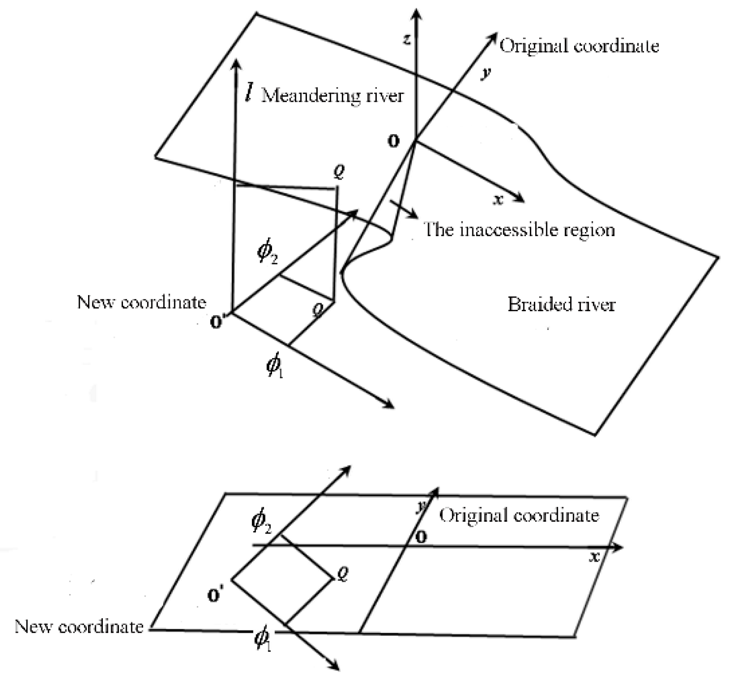
Based on the features of the topological relationship, the characteristics and the continuity of the equation can be maintained with the coordinate transformation. Translate the coordinate into the O′ (ϕ₁, ϕ₂, l), and obtain the following relationship for control parameters in the form:

$$\begin{array}{l}x=m_{1}l+m_2{\varphi }_1+m_3{\varphi }_2-{\varphi }_1{}^c\\ y=n_{1}l+n_2{\varphi }_1+n_3{\varphi }_2-{\varphi }_2{}^c\\ z=b_{1}l+b_2{\varphi }_1+b_3{\varphi }_2-l^c\end{array}$$

(11)

here x, y, z is the value of the coordinate in O′(ϕ₁, ϕ₂, l); b_i, m_i, n_i are the direction cosines between the original and new coordinate system. Substitute Equations (9)–(11) to Equation (4), the equation of the cusp catastrophe model under the new coordinate system O′(ϕ₁, ϕ₂, l) can be expressed as:

$$\begin{array}{ll}f(l,{\varphi }_1,{\varphi }_2)=& {(b_{1}l+b_2{\varphi }_1+b_3{\varphi }_2-l^c)}^3+(m_{1}l+m_2{\varphi }_1+m_3{\varphi }_2-{\varphi }_1^c)\\ & (b_{1}l+b_2{\varphi }_1+b_3{\varphi }_2-l^c)-(n_{1}l+n_2{\varphi }_1+n_3{\varphi }_2-{\varphi }_2{}^c)=0\end{array}$$

(12)

As shown in Figure 1, the rotation around the z-axis of the original coordinate to the coordinate system O′(ϕ₁, ϕ₂, l) contributes to b₁ = 1; and b_i, m_i, n_i satisfy the additional condition as:

$$\begin{array}{l}{m}_1^2+n_1^2+b_1^2=1\\ m_2^2+n_2^2+b_2^2=1\\ m_3^2+n_3^2+b_3^2=1\end{array}$$

(13)

The coordinate transformations satisfy the right-handed system:

$$\left|\begin{array}{ccc}{m}_1& m_2& m_3\\ n_1& n_2& n_3\\ b_1& b_2& b_3\end{array}\right|=1$$

(14)

Substitute Equation (13) to Equation (14), and obtain:

$$\begin{gathered} \gamma =\arctan l^c \\ \left|\begin{array}{ccc}{m}_1& m_2& m_3\\ n_1& n_2& n_3\\ b_1& b_2& b_3\end{array}\right|=\left|\begin{array}{ccc}0& \cos \gamma & \sin \gamma \\ 0& -\sin \gamma & \cos \gamma \\ 1& 0& 0\end{array}\right| \end{gathered}$$

(15)

There is no external force when the control parameters (ϕ₁, ϕ₂, l) equal to zero, the channel should maintain its pattern as Equation (12) and can be expressed as:

$$l^c{}^3-l^c{\varphi }_1{}^c-{\varphi }_2^c=0$$

(16)

Substitute Equations (14)–(16) into Equation (12), we have

$$f(l,{\varphi }_1,{\varphi }_2)={(l-l^c)}^3+l({\varphi }_1\cos \theta -{\varphi }_1{}^c)-{\varphi }_2(\sec \theta -l\cos \theta )+l^c{}^3=0$$

(17)

$$\theta =\arctan l^c$$

(18)

where ϕ^c₁, l^c is the critical index, assuming the critical value of state parameter denotes l^c = 1, and the critical transverse river-bed stability ϕ^c₁ = 1 when the rivers attain the equilibrium state.

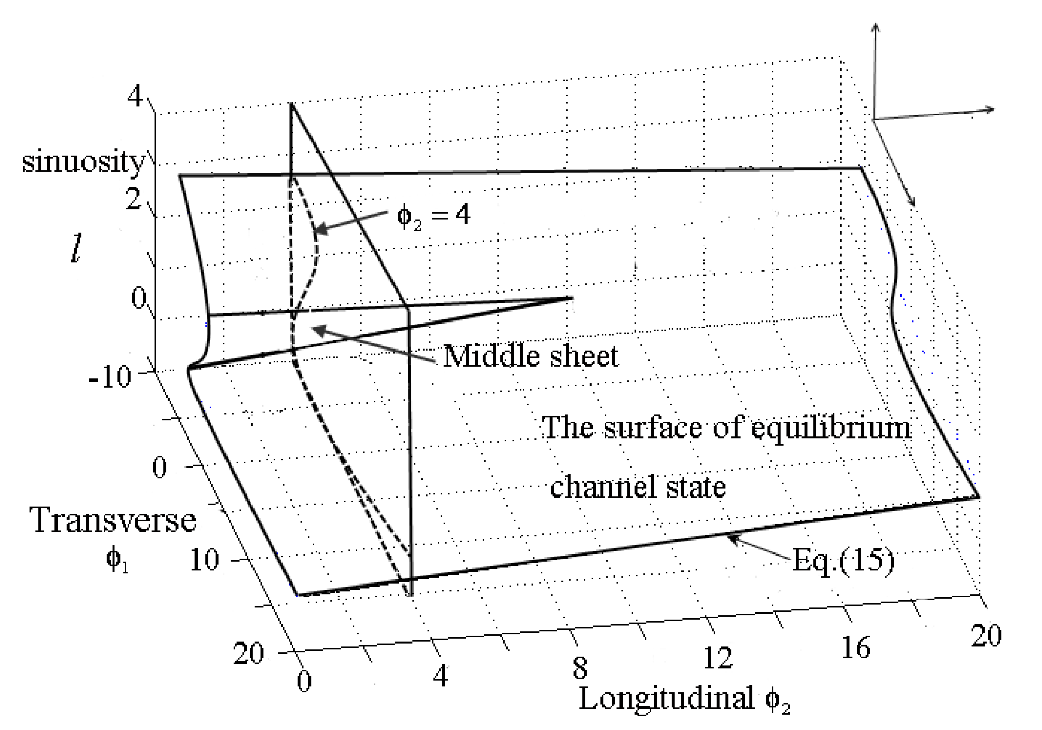
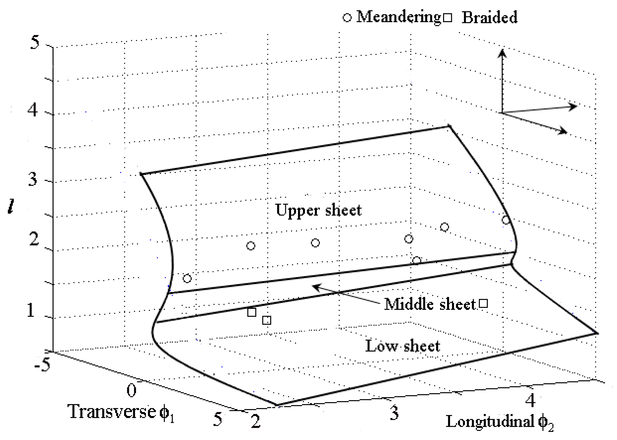
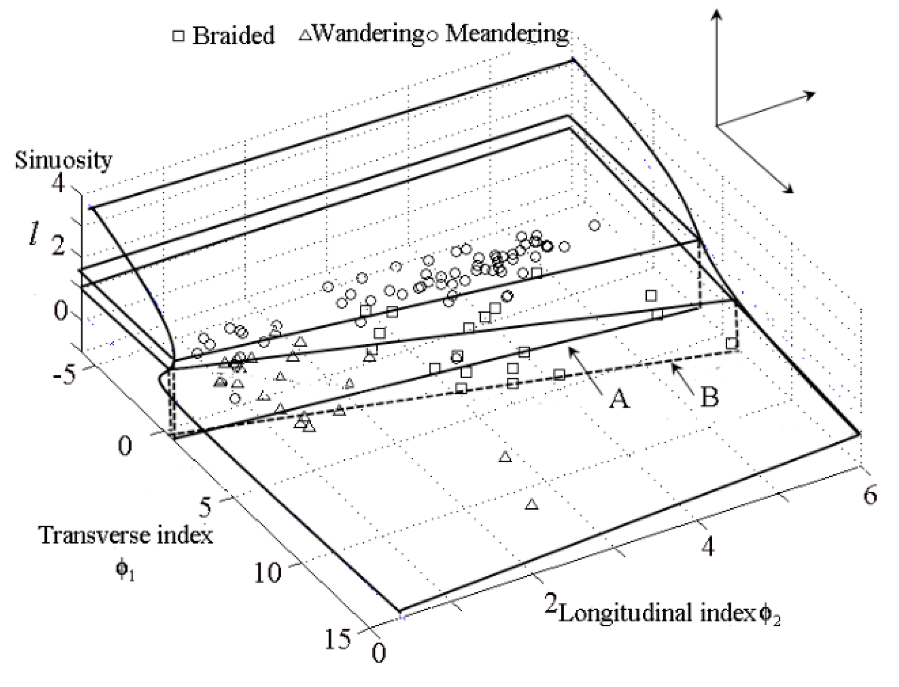
Equation (17) denotes the equilibrium state of the channel regime under the coordinate system O′ (ϕ₁, ϕ₂, l). The surface of equilibrium channel state in a 3-dimensional space is shown in Figure 2: the points located on the upper or lower sheet are minimal (steady equilibrium), a smooth change in (ϕ₁, ϕ₂) maintains the equilibrium state. The middle sheet, often referred as the inaccessible region, represents an unstable maximum [14]; if the rivers lie in this area, any slight alteration by a control parameter could result in the behavior being transferred to either the upper or lower sheet.

To investigate the applicability of the cusp model presented herein, the control parameters ϕ₁, ϕ₂ are obtained from a large dataset of natural rivers, including different types of channels as straight, meandering, and braided. The details of the river data are shown in

Table 1. Observed data of natural rivers.

Data Source	No	Width (m)	Discharge (m3/s)	D50 (mm)	Slope $(\times$1000)	Depth (m)	Sinuosity (-)
1.Andrews [33]	18	5.21–83.8	2.21–255	23–122	1.74–22.23	0.29–1.85	1.07–1.98
2.Church and Rood [34]	17	5–104	2.7–354	33–89	0.97–13.7	0.65–3.06	1.0–1.65
3.Hey and Thorne [35]	18	6.5–76.5	3.9–424	13.9–83.8	2.108–11.4	0.68–3.21	1.33–2.5
4.Kellerhals et al. [36]	24	18–442	7.93–2606	0.2–145	0.12–16.5	0.58–7.2	1.01–2.2
5.Lambeek [37]	4	111–450	1841–5320	12–73	0.22–1.6	3.8–10	1.1–1.7
6.McCarthy et al. [38]	1	137	630	0.35	0.4	4.1	1.86
7.Monsalve and Silva [39]	3	140–160	830–1200	0.4–6.2	0.24–0.8	3–5	1.2–2.5
8.Morton and Donaldson [40]	2	57–122	70–389	0.3–0.45	0.74–1.01	7–7.6	1.37–2.24
9. Taylor and Woodyer [41]	1	40	210	0.15	0.05	5.0	2.3
10. Mosley [42]	66	4.2–1753	1.73–3112	1.0–189	0.62–28.3	0.33–2.96	1.0–1.77
11. Williams [43,44]	4	13.7–57.9	12.2–365.3	2.7–42	1.52–6.9	0.7–3.38	1.32–1.93

.

Figure 3 shows the distribution of these rivers in the equilibrium surface: most points are on the other side of the surface, the structures are far from the equilibrium. It indicates that the internal adjustments are undergoing to reach the steady state in the dynamic system (Figure 3).

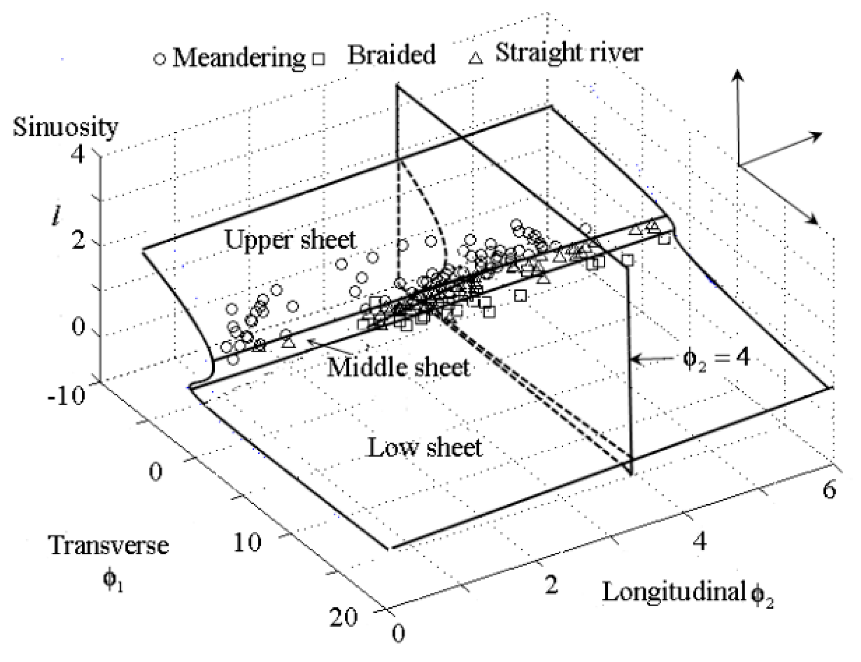
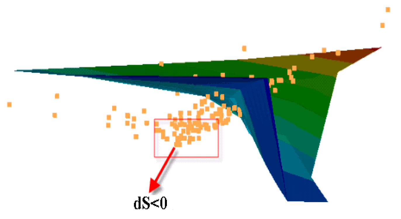
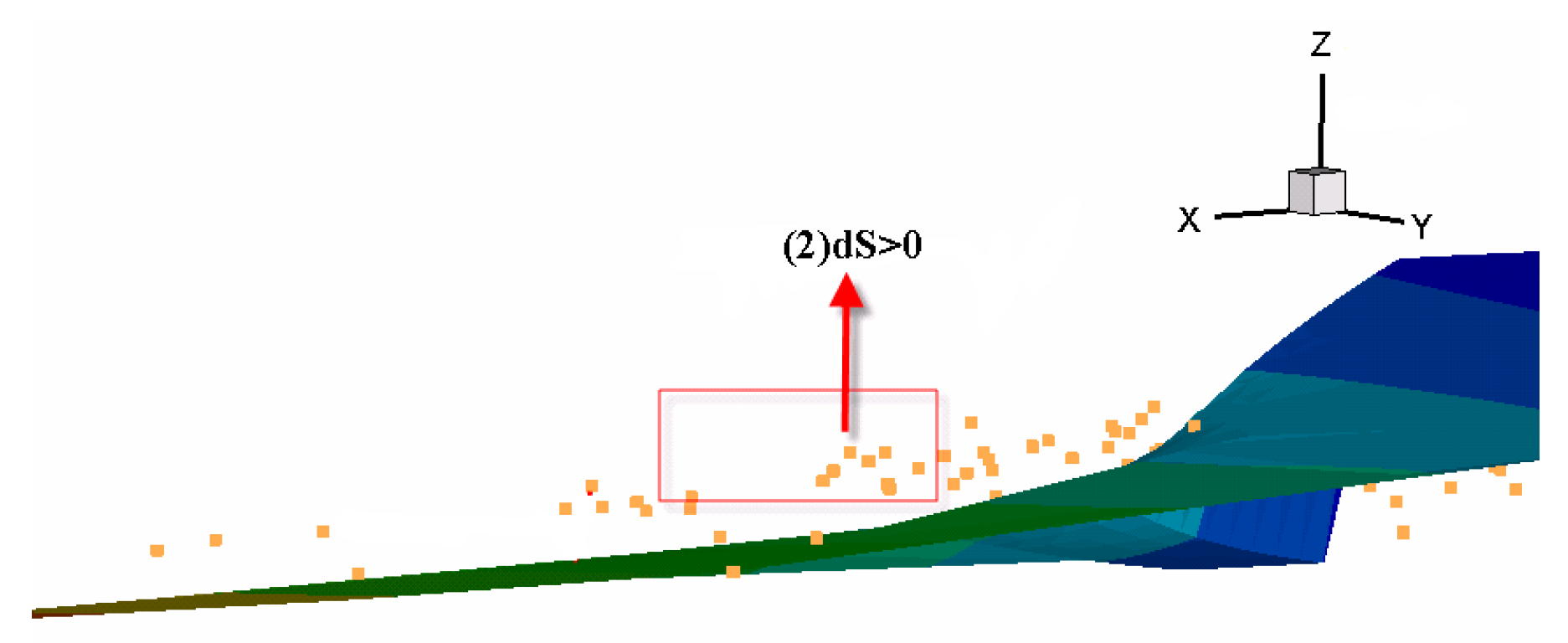
Combined with the dissipative structure theory and Equation (17), we can obtain the entry function, which implies that the system should achieve a stable surface at the expense of energy flowing into the system. Figure 4 shows that the sinuosity l will increase until the system reaches the surface. It indicates that the meandering river is a relatively stable pattern in nature, and this conclusion is proven and accepted by most of the researchers. If the entry function dS > 0, the system should be in a chaotic state at the second area; the system would reach the lower sheets as decreasing the sinuosity, it indicates the transition to unsteady braid river patterns with the expense of energy flowing out of the system (Figure 5).

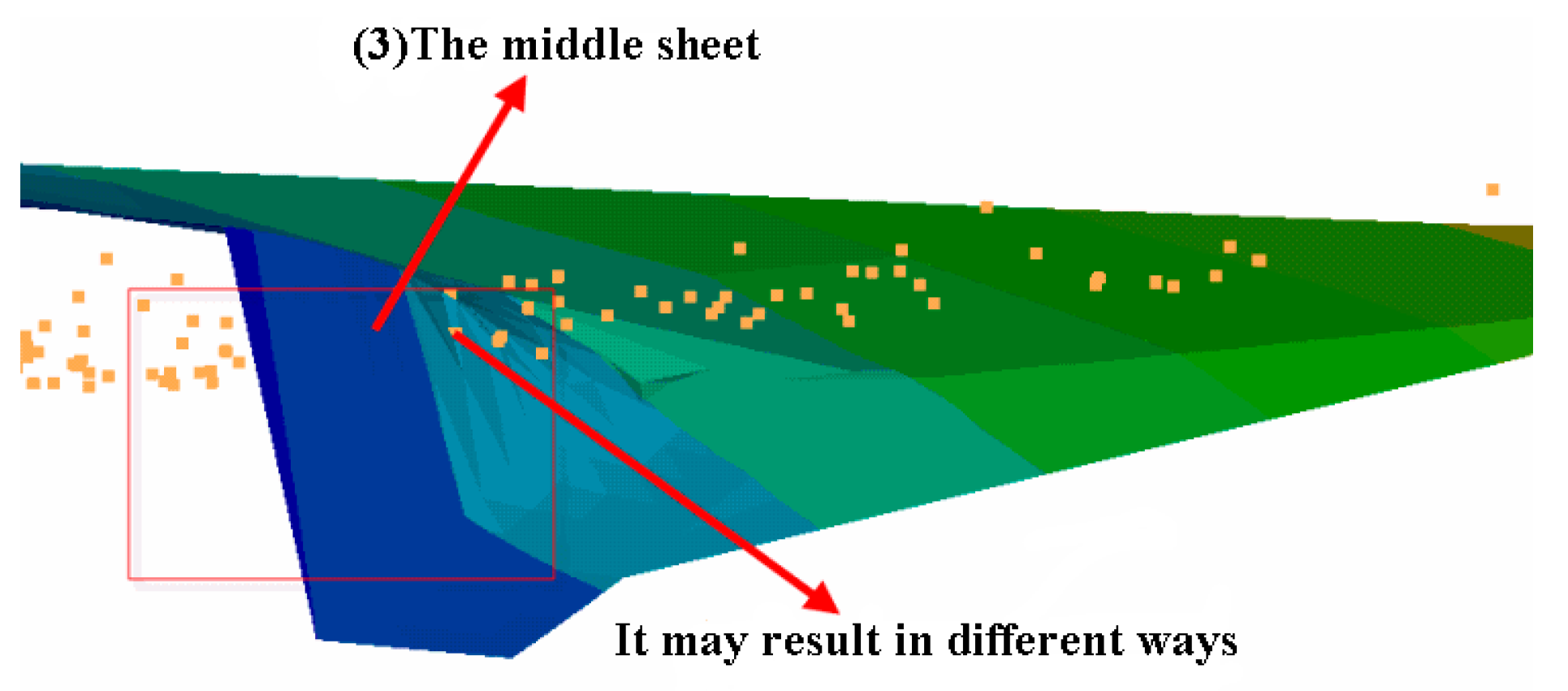
As shown in Figure 6, we can see a few points in the middle sheet, which is often referred to as the inaccessible region, representing an unstable maximum. All points along the fold curve are semi-stable points of inflection. The sinuosity l may either increase or decrease to reach the upper or lower sheet. It may result in two different stable states. These rivers may transfer to the meandering or unstable braided river in a slight alteration.

Figure 7 shows that 10 points are just on the equilibrium channel state surface (the values of ϕ₁, ϕ₂, l satisfy Equation (17)), either on the upper sheet or lower sheet (the global minimum). However, there are no points in the middle sheet (unstable maximum); it implies that the adjustments of alluvial channels tend to the minimum state, not an unstable maximum. The conclusion agrees qualitatively with the minimum entropy of the channel pattern theories [28]. There is no straight river on the equilibrium surface, which demonstrates that the straight pattern should not be included as one of the typical self-formed channel patterns [45].

The wandering river is wide, and the mainstream swings frequently; there are a large number of sandbars in the river channel, but the vegetation is scarce [46]. Based on the aforementioned cusp catastrophe model of alluvial channel regime, the data set of wandering rivers [46] are added to the channel state surface, and some suggestions about the channel stability can be obtained from Figure 8.

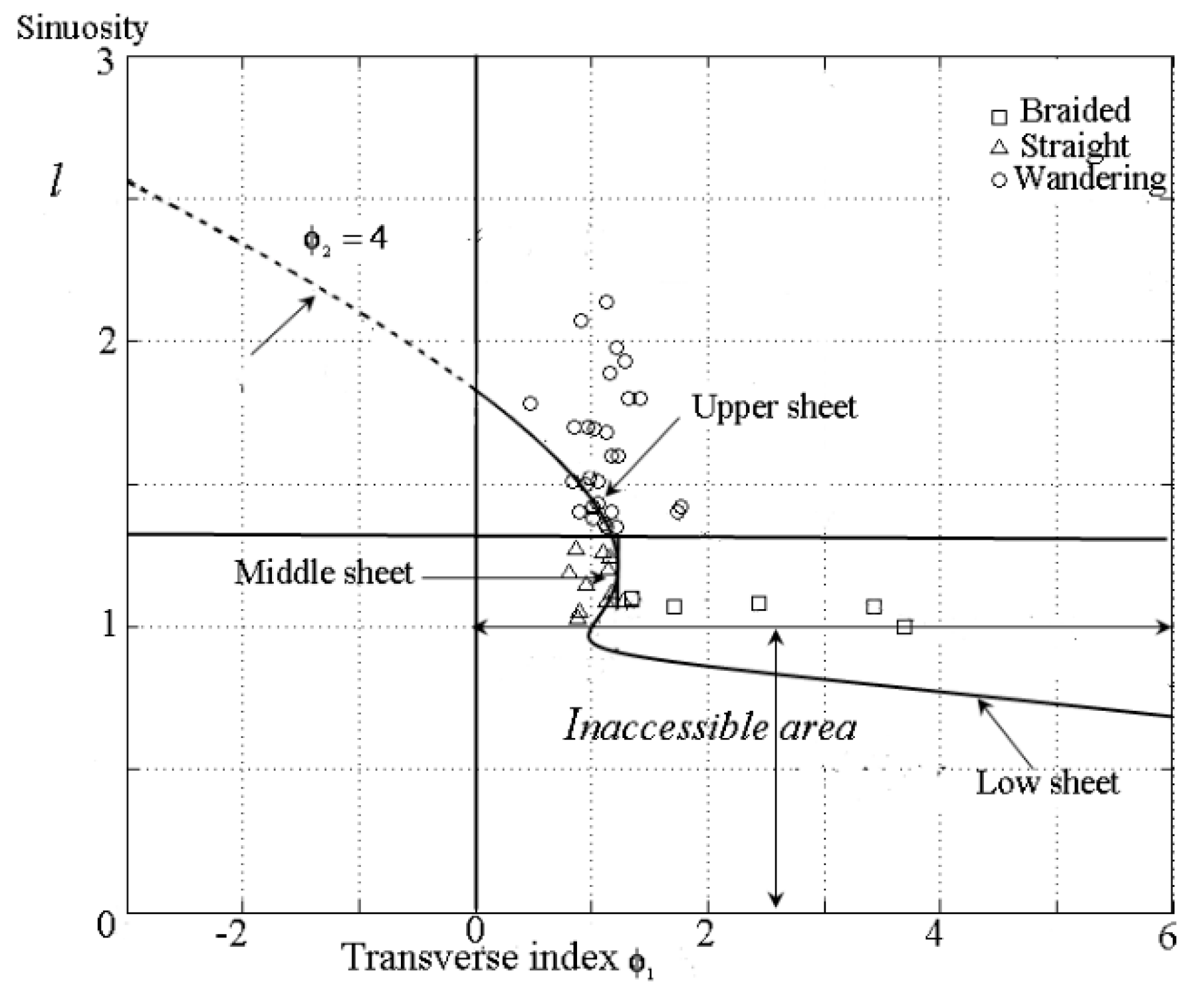
Choose the section ϕ₂ = 4 forward and backward about 0.5 units from the equilibrium surface (Figure 7), and the projection of the river points along the l-ϕ₁ plane is shown in Figure 8. The natural channels are scattered on either side of the intersection line which defines the control plane into three parts: the meandering, straight, and braided rivers belong to the upper, middle, and lower sheet, respectively; they may tend to achieve the intersection line by adjusting the control parameters ϕ₁, ϕ₂. Straight channels lied on the middle sheet represent an unstable maximum [39]; bifurcation may occur, and result in the meandering or braided channel pattern without external interference.

Over the short time scale, a channel can adjust its non-fluid boundaries to impose conditions in order to obtain and maintain steady-state equilibrium. Fluctuations occur during the self-adjustment of alluvial channels [11]. From Figure 8, we can assist in some suggestions for river management from the diagram. When the meandering channel with high sinuosity is far from the intersection line, the stability can no longer be maintained and a cut-off may occur to reach a new balance. In order to prevent the unfavorable impact of river stability change in practice, we should enhance channel stability to control the pattern. If the channels are just around the intersection line, the channel pattern can be maintained if the condition of flow discharge and sediment is constant.

Based on the definition of the state parameter as sinuosity l, the region in the lower sheet is inaccessible (Figure 8); the channels belong to braided patterns, the width and the width-depth ratio of these channels are relatively large according to the field data (

Table 2. Observed data of natural braided rivers.

River Reach	Width (M)	Slope $(\times$1000)	Depth (M)	Width to Depth Ratio (-)	Control Parameters
					ϕ1	ϕ2
Rakaia	1753	4.04	0.84	2086	3.69	3.50
2 Grey	124	3.41	1.86	66.7	1.34	4.26
3 Waiau-Uha	1156	4.9	0.78	1482	3.4	3.90
4 Hakataramea	390	5.9	0.67	573.5	2.8	3.50
5 Ohau	109	6.9	0.84	129.7	1.71	3.55

). Deviations from equilibrium conditions will trigger the decrease of the control parameter ϕ₂ to attain the available balance with the response between inflowing and outflowing water and sediment discharge, such as decreasing the slope or width-depth ratio.

2.4. The Cusp Catastrophe Model for the Channel Pattern Classification

Numerous descriptive classification schemes have been proposed [47] as well as differences in stability and sedimentation controls in alluvial rivers. Based on the cusp model of alluvial channel regime, a new channel pattern classification is presented according to the channel stability in this section. The discriminant functions are obtained from the model to distinguish the channel patterns. The validity of the proposed method is tested with the river data from Table 1.

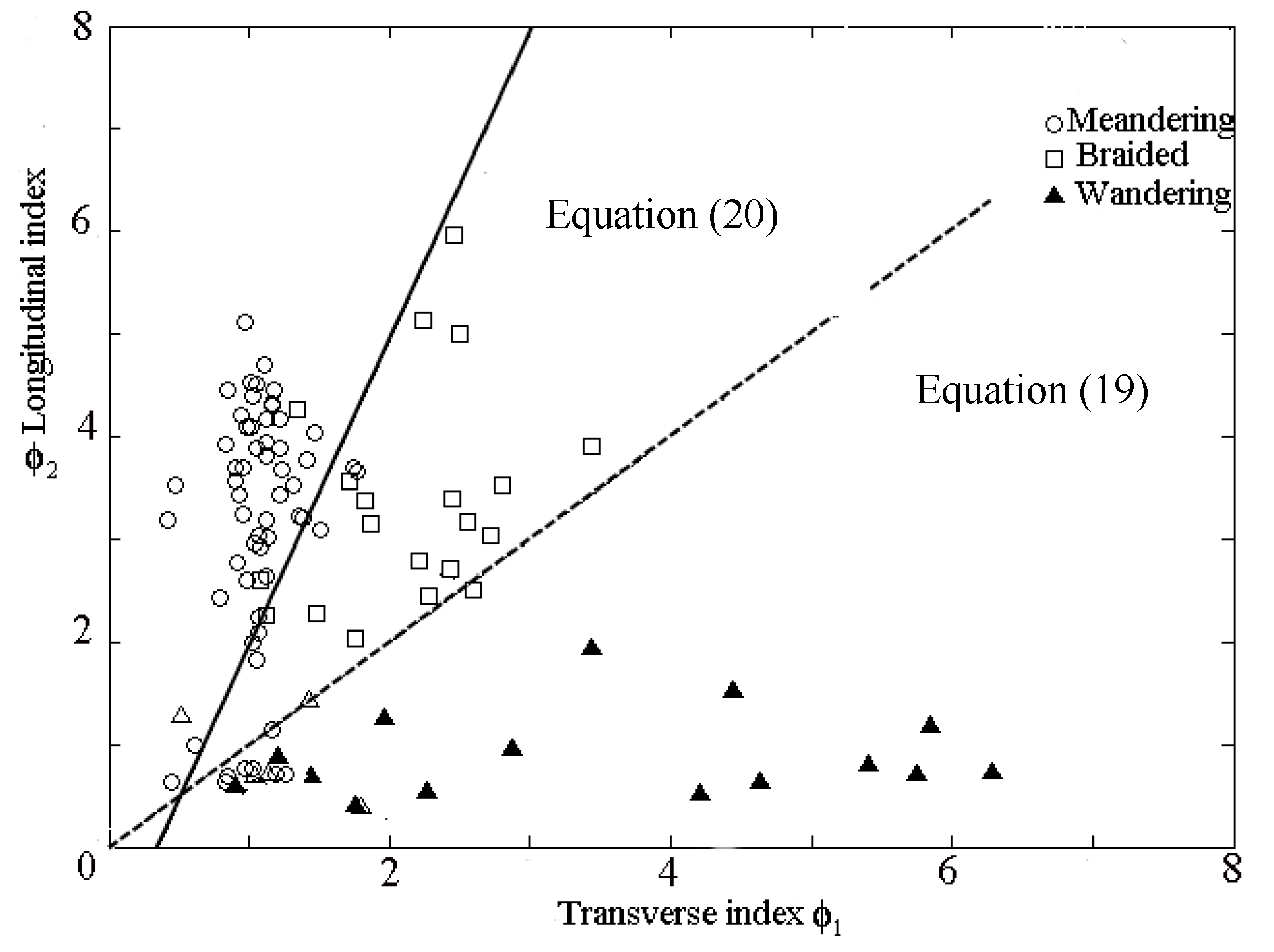
The cusp catastrophe model of alluvial channel regime can reflect the stability of the rivers; one can see the channels achieve to the prescribed minimum of equilibrium state when L = 1; the value of sinuosity in excess of 1.5 is often used to discriminate the meandering and braided rivers [48]. The cross-sections of L = 1 and L = 1.5 are used to divide the equilibrium surface, as shown in Figure 9, and brought into Equation (17), the discriminators are derived as:

$$\mathrm{When}\mathrm{L}=1:{\varphi }_1-{\varphi }_2=0$$

(19)

$$\mathrm{When}\mathrm{L}=1.5:{\varphi }_1-{\varphi }_2/3=0.35$$

(20)

The 2D projection of the natural channel (Figure 6) along the control ϕ₁–ϕ₂ plane can be sketched in Figure 10. Discriminator (20) represents a reasonable lower bound for wandering channels (the data for wandering channels come from Zhang et al. [46]). Discriminator (19) forms a reasonable upper bound for the meandering channels; braided rivers by the definition used in this analysis, or should at least be regarded as transitional forms based on the dynamic features, and they are in the region between Discriminators (19) and (20) in this diagram. The control plane is divided into three zones: the upper zone, which can be regarded as the stable zone; the middle zone, defined as the transitional stable zone; and the unstable lower zone. It indicates that the classification diagram is in agreement with the known channel pattern theories from the stability feature. Substitute Equations (6) and (7) to the Discriminators (19) and (20), the discriminant function that predicts the channel pattern can be derived as follows:

Meandering channel:

$${\left(\frac{({\gamma }_s-\gamma )D_{50}}{\gamma hJ}\right)}^{1/2}>3{\left(\frac{B{J}^{0.2}}{Q^{0.5}}\right)}^{1/2}-1.05$$

(21)

Braided channel:

$${\left(\frac{B{J}^{0.2}}{Q^{0.5}}\right)}^{1/2}<{\left(\frac{({\gamma }_s-\gamma )D_{50}}{\gamma hJ}\right)}^{1/2}<3{\left(\frac{B{J}^{0.2}}{Q^{0.5}}\right)}^{1/2}-1.05$$

(22)

Wandering channel:

$${\left(\frac{B{J}^{0.2}}{Q^{0.5}}\right)}^{1/2}<{\left(\frac{({\gamma }_s-\gamma )D_{50}}{\gamma hJ}\right)}^{1/2}$$

(23)

As shown in Figure 10, the channel patterns are difficult to distinguish nearby the origin, according to the catastrophe theory: the region around the origin of the fold line could have remarkably different outcomes of the system behavior. For although the two paths may begin close together, their paths are divergent [26], which can be used to explain that the different planforms may result from the same sediment-discharge and boundary conditions.

3. The Discriminant Function for the Alluvial Channel Stability

3.1. Establishment of the Discriminant Function

The stability of a channel is related to the bed material movement [49]. When the river achieves a stable state, the bed material begins the incipient motion. The critical longitudinal index ϕ_b^c can be expressed as:

$${\varphi }_b^c=\frac{U{*}_c^2\rho }{({\gamma }_s-\gamma )D_{50}}={\theta }_{\mathrm{c}}$$

(24)

where θ_c is the critical shield’s number for the incipient motion.

The river width is equal to that under the bank-full discharge when the river is in an equilibrium state. The critical traversal index (7) can be expressed as ϕ_h^c = 1.

The relative traversal and longitudinal indexes ϕ₁′, ϕ₂′ are applied as the control factors, and the relative sinuosity l’ is the state parameter in the cusp catastrophe model to describe the river stability. The control factors and state parameter can be written as:

$${\varphi }_1^{\prime }={\varphi }_{\mathrm{h}}^c-{\varphi }_h=1-\frac{B{J}^{0.2}}{Q^{0.5}}$$

(25)

where ϕ₁^′ reflects the traversal stability of a river.

$${\varphi }_2^{\prime }={\varphi }_b^c-{\varphi }_b={\theta }_c-\frac{\gamma hJ}{({\gamma }_s-\gamma )D_{50}}$$

(26)

where ϕ₂^′ reflects the longitudinal stability of a river.

$$l^{\prime }=l_c-l$$

(27)

where l′ reflects the variation in the sinuosity between the stable and the local statue, l_c, l is the sinuosity of a river in the stable and local state, respectively.

Bring Equations (25)–(27) to the equilibrium Equation (5), and the stability equation for the channel can be obtained as:

$$4l^{\prime 3}+2l^{\prime }(1-\frac{B{J}^{0.2}}{Q^{0.5}})+({\theta }_c-\frac{\gamma hJ}{{\gamma }_s-\gamma })=0$$

(28)

Cardan’s discriminant function (6) can be written as:

$$\Delta =8{(1-\frac{B{J}^{0.2}}{Q^{0.5}})}^3+27{({\theta }_c-\frac{\gamma hJ}{({\gamma }_S-\gamma )D})}^2$$

(29)

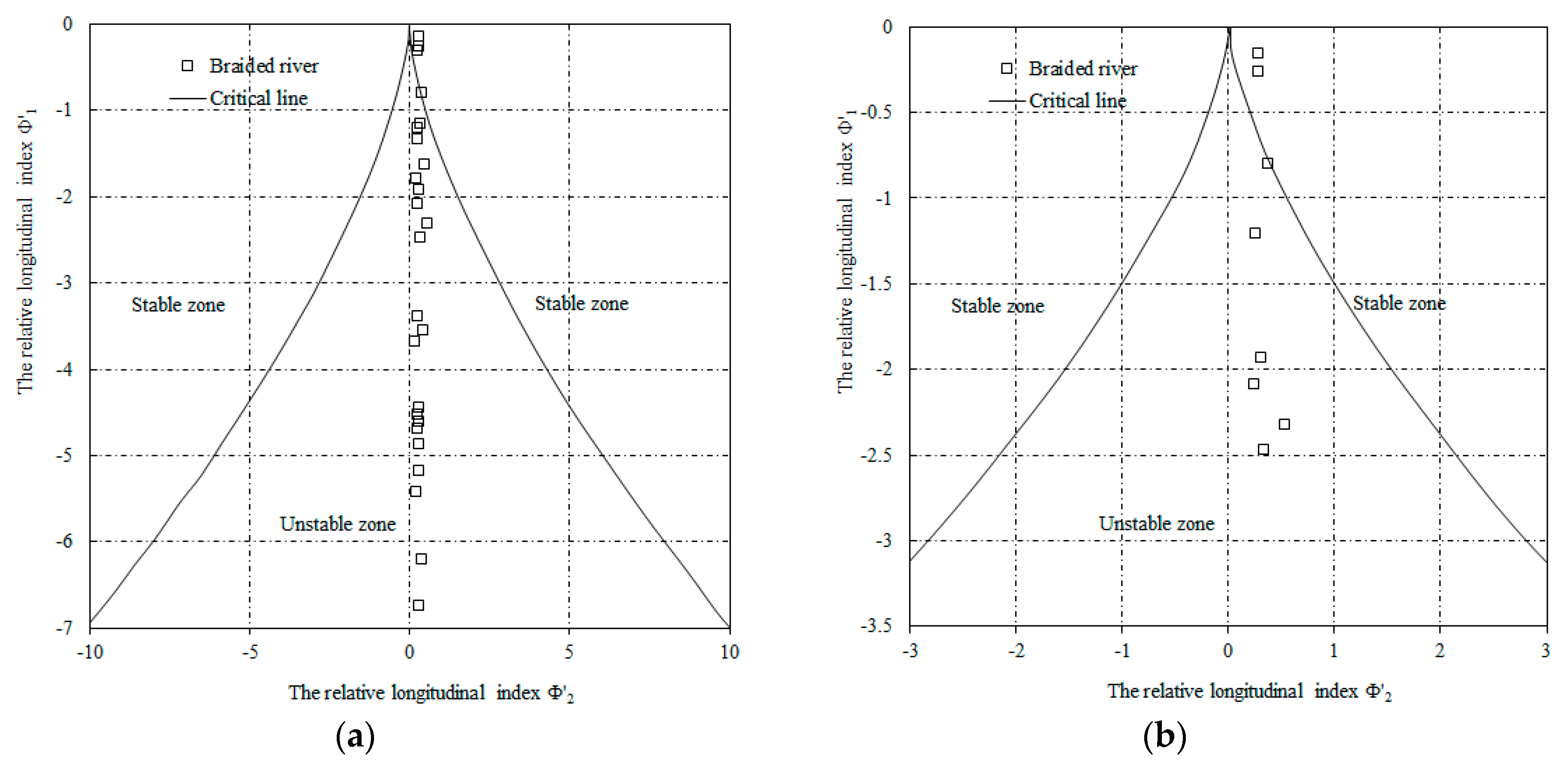
where $\Delta$ can reflect the river state; if $\Delta >0$, the river is in a stable stage; if $\Delta <0$, the river is in a unstable condition; and if $\Delta =0$, the river is in a critical stable state, a small disrupt may lead to a change in the channel geometry.

3.2. Verification of the Discriminant Function

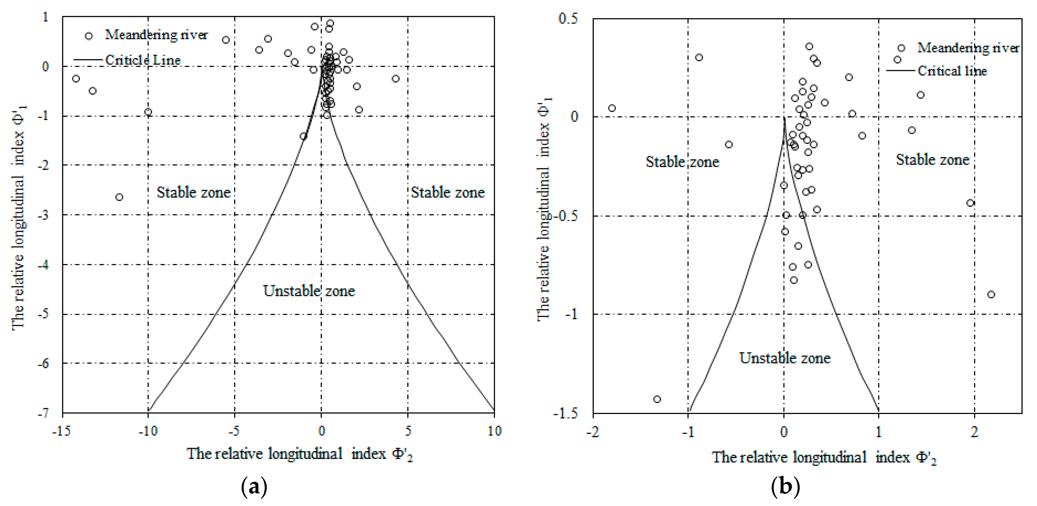
The data set of the natural rivers are from Table 1 and Zhang et al. [46]. According to the developed classification of the channel pattern, the control factors ϕ1′, ϕ2′ for the meandering, straight, and braided channel were calculated and brought into discriminate function (29). The results can be seen in Figure 11, Figure 12 and Figure 13.

Figure 11a shows that most of the meandering channel are in the stable zone. That is, the river can maintain the current state for a long time. There are still a few meandering rivers nearby the critical line in Figure 11b; some of them are in the unstable zone. In practice, we can adjust the control factors to make all of the channels tend to the equilibrium state, for example, an increase of the flow discharge can lead to a decrease in the distance from the relative longitudinal index to the stable zone.

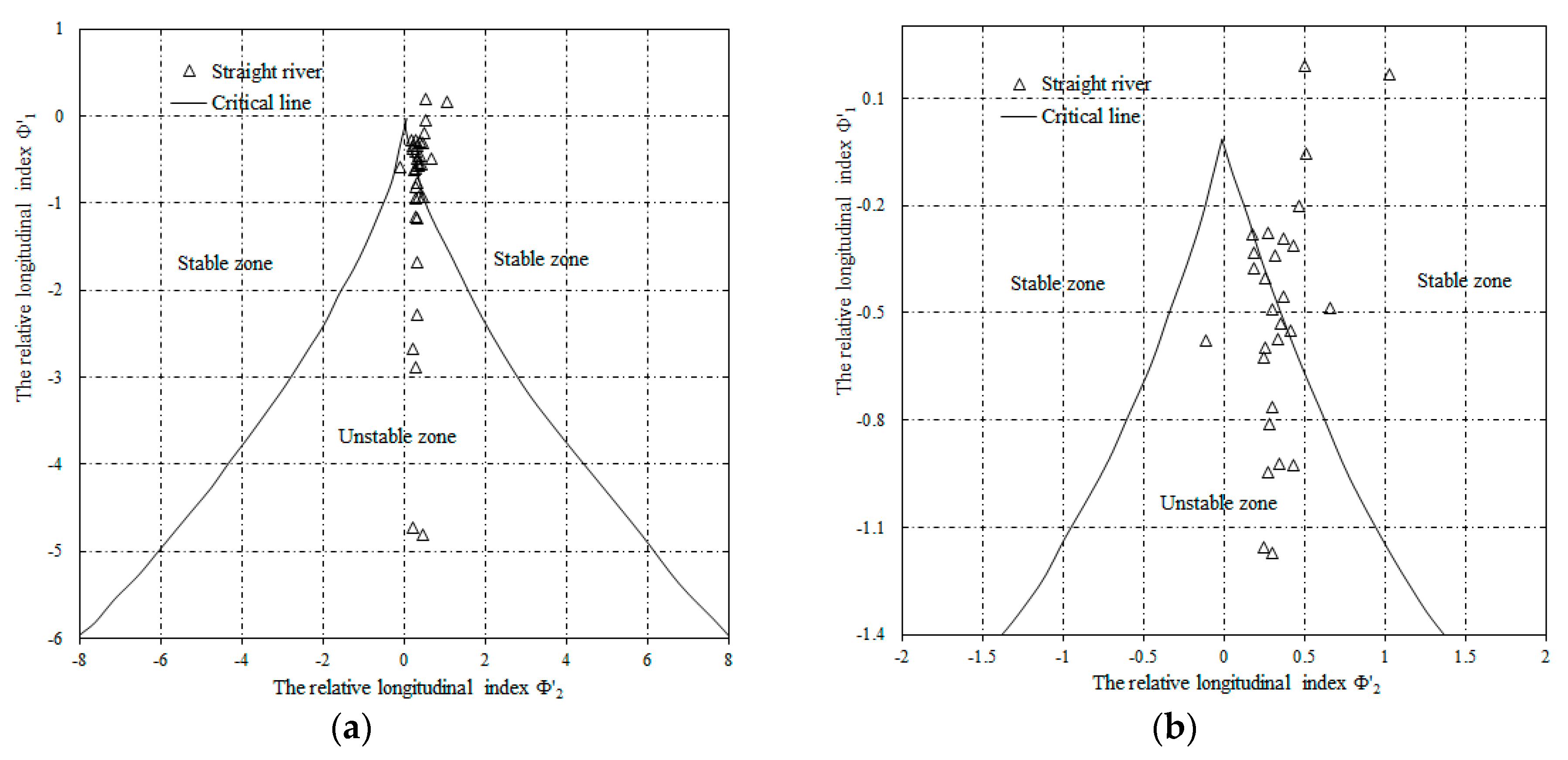
Figure 12 shows that almost the straight channels are nearby the critical stable lines; it implies that the river may enter into an unstable zone with a tiny change. We need to focus on the changes of the control factors to ensure river stability. It can be seen that the braided channels are almost in the unstable zone (Figure 13). However, there are still a few meandering channels in the unstable zone, and some of the straight channels in the stable area (Figure 11 and Figure 12).

We choose point A Selwyn River located in the critical line (Figure 11b) and point B Buller River in the stable zone (Figure 12b) to investigate the state of the channel. The related parameters for the stability of the two rivers can be seen in

Table 3. Field data of Hamps channel.

River Section	Φ1 ′	Φ2 ′	Δ
Selwyn River	−0.75	0.24	−1.8
Buller River	0.48	0.64	10.33

. According to the research on the fluvial process in the Selwyn River, the river is in a change between the braided and meandering pattern because of the influence of the inlet flow-sediment discharge and bank vegetation [50,51]. Buller River is the largest river in New Zealand; although the channel pattern is straight, the clay bank materials and vegetable cover contribute to the stability of the bank, and the river keeps the stable state. These results are in agreement with the field data, and illustrate that the channel pattern can not determine the river stability.

It should, however, be noted that the state of the river is not illustrated in Table 1. In order to test the discriminate function, we adopted the field data from 20 naturally stable channels in the UK [52]. The calculated values of the discriminate function can be seen in

Table 4. Results with field data of natural stability channels in the UK.

River Section	Φ1 ’	Φ2 ’	Δ
Teviot at Hawick	0.081652675	0.421672464	2.077705394
Exe at Stoodleigh	−0.146498713	0.479981148	3.157327172
Usk at Llandetty	0.306517002	0.531238705	4.799550439
North Tyne at Tarset	0.171287961	0.486915852	3.351635451
Tweed at Peebles	−0.025386507	0.565425868	4.885953245
Yscir at Pontaryscir	0.185434467	0.480383884	3.268241467
Sprint at Sprint Mill	−0.151169956	0.353716859	1.377717415
Yarrow Water at Philiphaugh	−0.211474561	0.359206172	1.609168992
Alwin at Clennel	−1.279978326	0.254689138	13.55281793
Coquet at Bygate	−1.953615324	0.3461899	31.65313202
Snaizeholme Beck	−0.633915741	0.425806949	5.299293804
Rede at Rede’s Bridge	−0.924715868	0.427212477	8.946006101
Glaslyn at Beddlegert u/s	−0.037797355	0.37255358	1.407572393
Glaslyn at Beddlegert d/s	−0.893945136	0.37186106	7.78147533
Tarsetburn at Greenhaugh	0.150349187	0.478402527	3.137109449
Fowey at Restormel	−0.076519308	0.535205284	4.186122941
Hodder at Hodderplace	−0.045766839	0.480741662	3.016603416
Esk at Cropple How d/s	−0.109785644	0.486580798	3.206912053
Erme at Ermington	0.200651184	0.269685306	0.85167211
Otter at Dotton	−0.022693634	0.42746865	2.113119973
Dyfyrdwy at New Inn	0.123405107	0.484106991	3.185118538
Alwen at Druid	−0.189059856	0.427541334	2.396024985
Lugg at Byton u/s	−0.36688634	0.41404418	2.993322602
Lugg at Byton d/s	−0.048668144	0.418682887	2.000564222
Manifold at Hulme End	−0.803954047	0.373945434	6.582586586
Glendaramackin at Threlkeld	0.302536456	0.376950845	2.178391725
Tweed at Lyneford	−0.068990566	0.530561351	4.070542484

. The values are all larger than 0, and the results imply that the rivers are in a stable state, which agrees well with the measured data.

According to the verification with the measured data of 120 natural rivers, the discriminate function can quantitatively distinguish river stability, and give some assistance in river management and regulation.

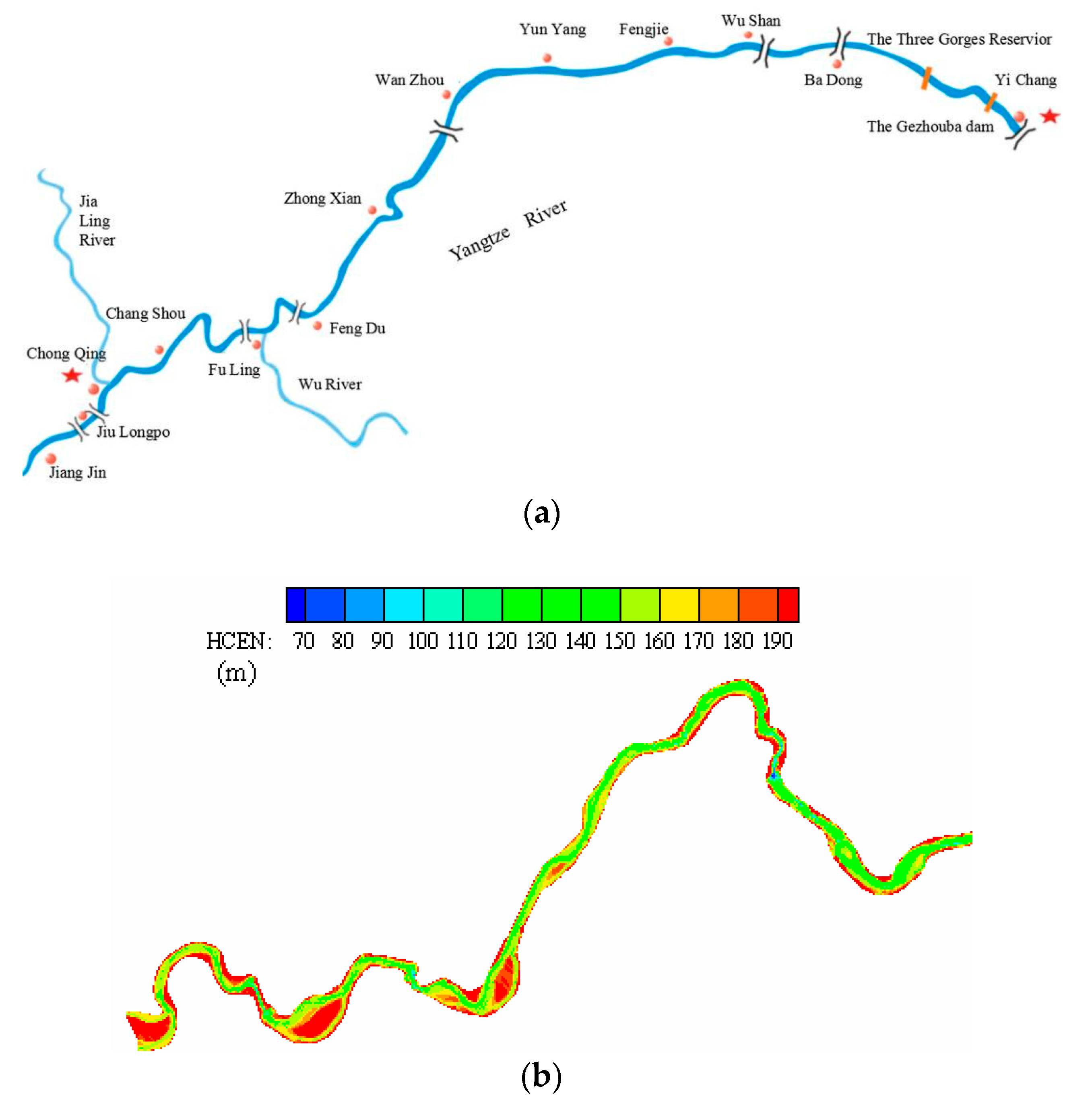
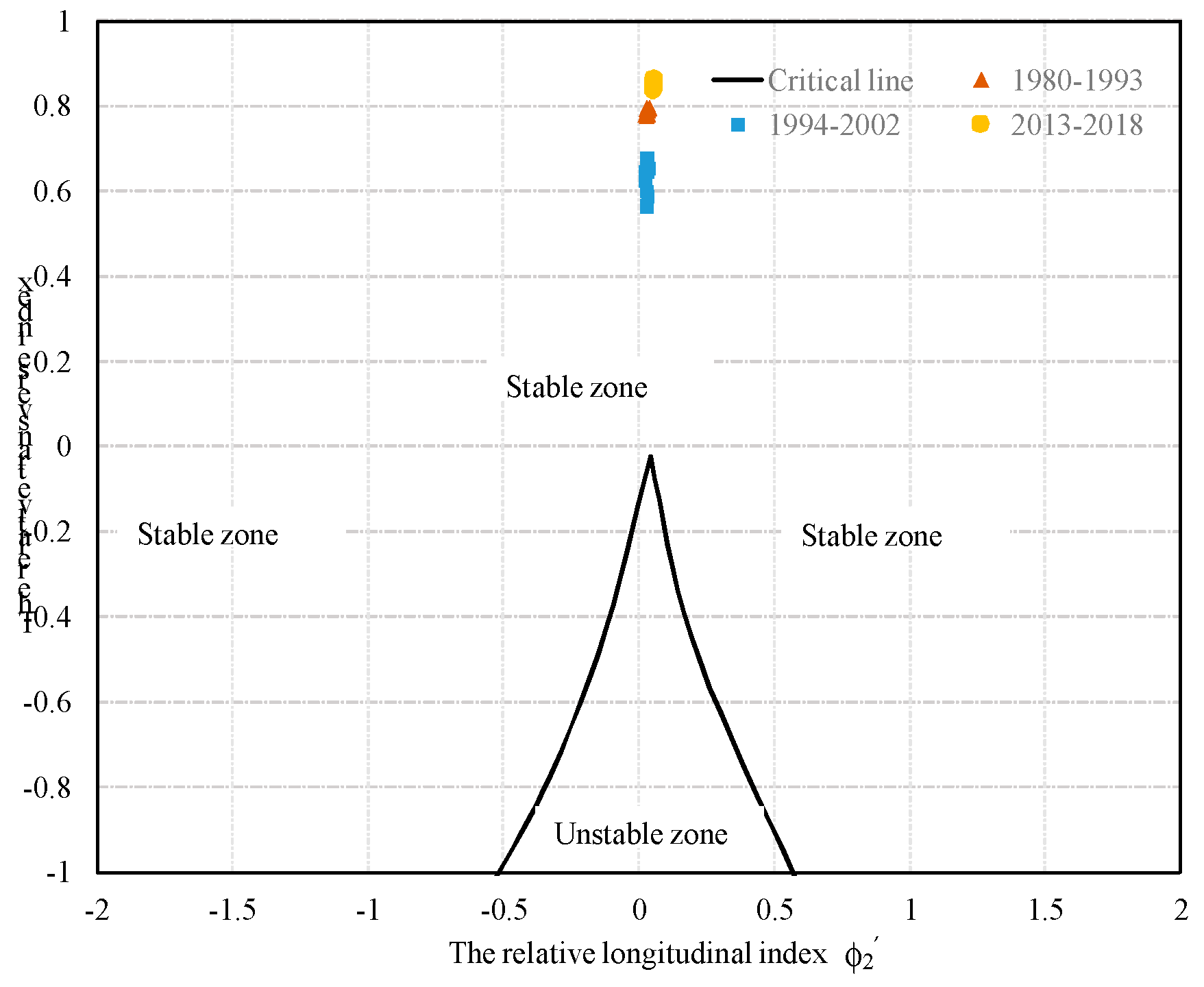
4. Application to the Upstream of the Yangtze River, China

The model is used to investigate the channel pattern and state of the typical river reach in the upstream of the Yangtze River. The study area is approximately 140 km long, stretching from Fuling to Chongqing (Figure 14a). As we know, the Three Gorges Dam (TGD) was brought into operation in 2003; the river reach in Chongqing-Fuling (CF) is in the fluctuating backwater area (Figure 14b). This study is based on an extensive dataset of the mean annual water discharge Q, river width B, and river slope J from 1980 to 2018, collected from the control hydraulic stations along the river reach [53]. The grain size D50 of the river bed material is obtained from the core documents [54].

4.1. The Temporal Changes of the Channel Pattern

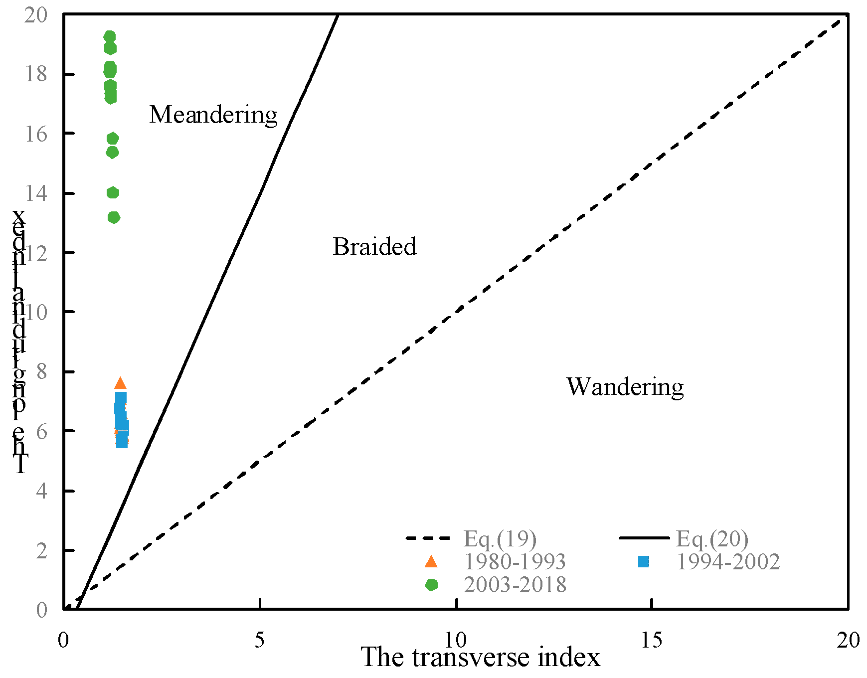
The control factors ϕ1, ϕ2 proposed in Section 2 are calculated and plotted in the classification diagram. Considering the TGD construction, we divided the years into the series of 1980–1993, 1994–2002, and 2003–2018, which are the before, undergoing, and operation stages of the TGD. Figure 15 shows the temporal change of the channel pattern for the past three decades. The three groups locate in the meandering zone, indicating that the plane form of the river reach maintains its channel pattern for decades, which is consistent with the actual condition [54]. The result indicates that river engineering can not alter the channel pattern in the decadal timescale. As shown in Figure 15, the position of the points after 2002 is far away from the ones before the TGD operation. The result indicates that the water surface slope J of the study area decreases with the operation of the TGD, and leads to a decline in the water power in the backwater zone [55].

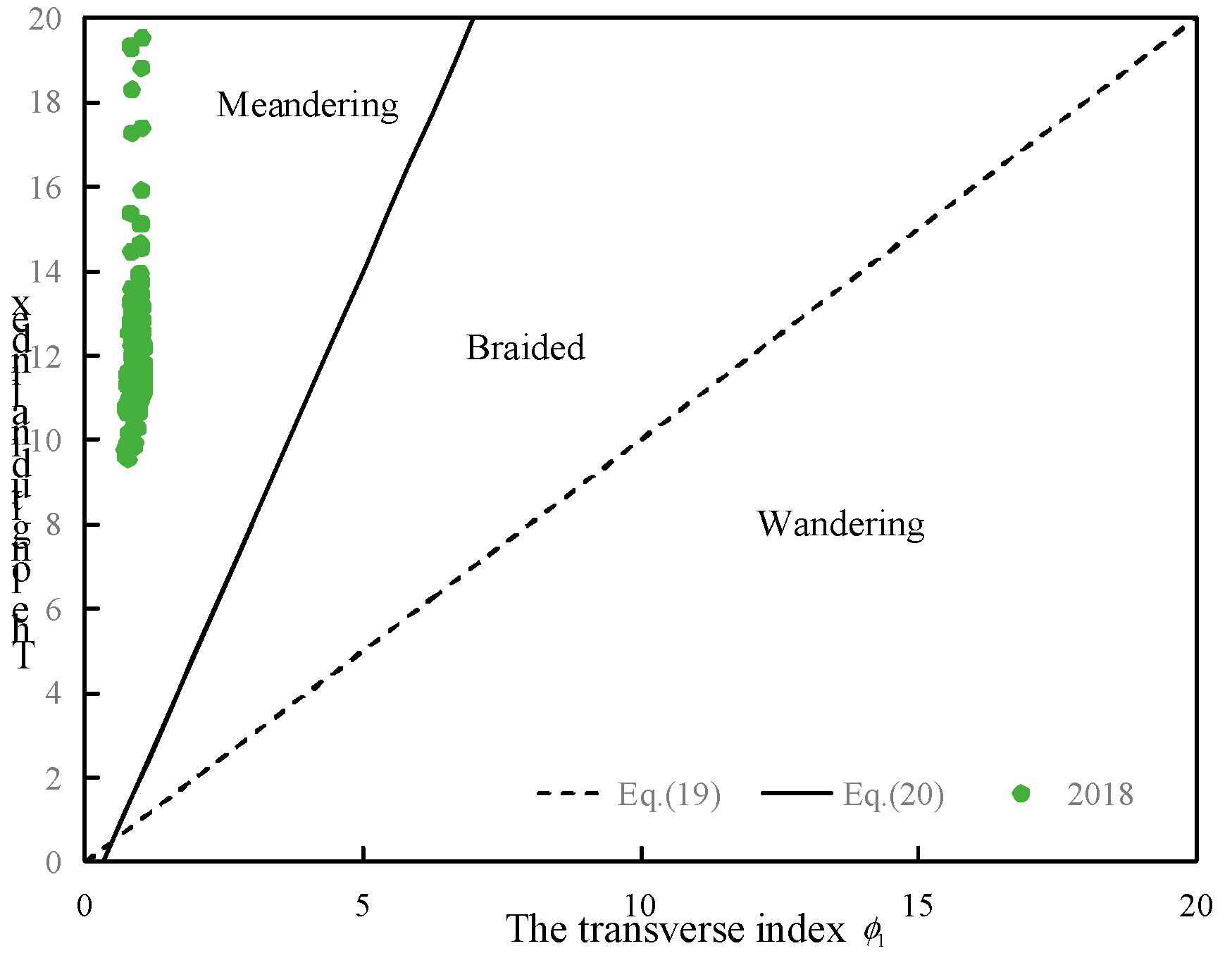
Then, we chose the dataset of daily river conditions to investigate the change trends of the channel pattern in one year (2018), and the river bed material condition adopted three values for the dry, medium, and flood discharge stages [54]. Figure 16 shows that the scatter points are still in the meandering zone, although the river condition varies over the days. The aforementioned results imply that the change of the channel pattern depends mainly on the geological, climate, and tectonic processes [56].

4.2. The Temporal Changes of the River Status

Based on the aforementioned dataset of the river conditions in the study area, we calculated the relative control factors ϕ₁′, ϕ₂′. Figure 17 shows the status of the river reach over the past three decades. As seen, the river reach in the upstream of the Yangtze River kept its stable state in the past three decades, and the stable trend will be maintained in the future. The points before 2002 are in a stable area, far away from the threshold lines. When the TGD was in the construction stage between 1994 to 2003, the distances between the points and the critical lines decrease, implying that river engineering can influence the stability of the river state. After the establishment of the TGD, the points returned to the original position of the time-series from 1980 to 1994, indicating that the adjustment of the river dynamic process tends to a stable condition, which agrees well with the in situ measurements [55].

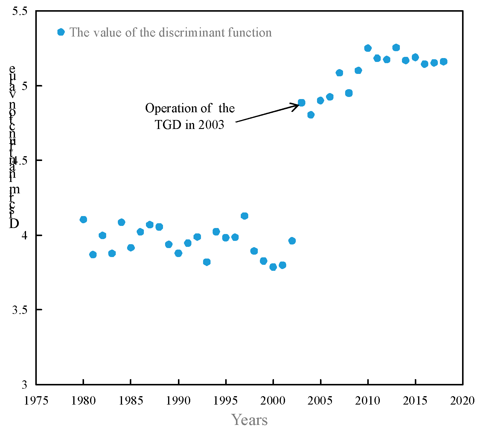
We calculated the values of the discriminant function Δ for river stability and obtained the diagram to investigate the changing trend of the river stability with time (Figure 18). The result demonstrates that the change process of stability was influenced by the TGD project, and agrees well with the aforementioned conclusion from Figure 17.

5. Conclusions

This paper presents a cusp catastrophe model for alluvial channel regime with suitable parameters to determine the river channel and the channel stability. Equations of equilibrium state and channel patterns are established based on the model of cusp catastrophe surface by selecting suitable parameters. The channel patterns can be identified by such a model in a direct way with a quantified index, which is a cusp catastrophe surface in a translated 2D dimensional coordinate, and the discriminant functions are obtained from the model to distinguish channel stability. Predictions based on this model are consistent with field observations involving 150 natural rivers of small or medium sizes. Then, the proposed model was applied to the typical river reach in the upper reaches of the Yangtze River, and the results were compatible with the field measurements. The results indicate that this method may be applied to study the regime of natural rivers and to assist decision-making in river management. However, some assumptions were proposed during the model establishment; further studies are needed to improve understanding of the patterning process and modify the control parameters in the cusp catastrophe model.

References

- Hossein, A.; Mohammad, A.; Singh, V.P. Hydraulic Geometry Relations for Stable Channel Design. J. Hydrol. Eng. 2010, 15, 859–864. [Google Scholar]
- Van der Berg, J.H. Prediction of alluvial channel pattern of perennial rivers. Geomorphology 1995, 12, 259–279. [Google Scholar] [CrossRef]
- Millar, R. Theoretical regime equations for mobile gravel-bed rivers with stable banks. Geomorphology 2005, 64, 207–220. [Google Scholar] [CrossRef]
- Farias, H.D.; Pilan, M.T.; Mattar, M.T.; Pece, F.J. Regime width of alluvial channels: Conciliation of several approaches. In Proceedings of the ICHE Conference, Cottbus, Germany, 1998. [Google Scholar]
- Singh, V.P.; Yang, C.T.; Deng, Z.Q. Downstream hydraulic geometry relations: 1. Theoretical development. Water Resour. Res. 2003, 39, 2145–2161. [Google Scholar]
- Bizzi, S.; Lerner, D.N. The Use of Stream Power as an Indicator of Channel Sensitivity to Erosion and Deposition Processes. River Res. Appl. 2013, 31, 16–27. [Google Scholar] [CrossRef]
- Mao, L.L.; Chen, Y.M. Entropy-Based approach of hydraulic geometry of navigable canals. J. Hydrol. Eng. 2018, 23, 04018047. [Google Scholar] [CrossRef]
- Song, X.L.; Zhong, D.Y.; Wang, G.Q. A study of the stochastic evolution of hydraulic geometry relationships. River Res. Appl. 2019, 33, 867–880. [Google Scholar] [CrossRef]
- Alabyan, A.M.; Chalov, R.S. Types of river channel patterns and their natural controls. Earth Surf. Process. Landf. 1998, 23, 467–474. [Google Scholar] [CrossRef]
- Nelson, A.; Dubé, K. Channel response to an extreme flood and sediment pulse in a mixed bedrock and gravel-bed river. Earth Surf. Process. Landf. 2015, 41, 178–195. [Google Scholar] [CrossRef] [Green Version]
- Montgomery, D.R.; Buffington, J.M. Channel-reach morphology in mountain drainage basins. GSA Bull. 1997, 109, 596–611. [Google Scholar] [CrossRef]
- Brierley, G.J.; Fryirs, K.A. River Styles, a geomorphic approach to catchment characterization: Implications for river rehabilitation in the Bega catchment, New South Wales, Australia. Environ. Manag. 2000, 25, 661–679. [Google Scholar] [CrossRef]
- Gurnell, A.M.; Rinaldi, M.; Belletti, B.; Bizzi, S.; Blameur, B.; Braca, G. A multi-scale hierarchical framework for developing understanding of river behaviour to support river management. Aquat. Sci. 2016, 78, 1–16. [Google Scholar] [CrossRef] [Green Version]
- Fryirs, K. River sensitivity: A lost foundation concept in fluvial geomorphology. Earth Surf. Process. Landf. 2017, 42, 55–70. [Google Scholar] [CrossRef]
- Beechie, T.; Imaki, H. Predicting natural channel patterns based on landscape and geomorphic controls in the Columbia River basin, USA. Water Resour. Res. 2013, 44, 1390–1406. [Google Scholar]
- Nicholas, A.P. Modelling the continuum of river channel patterns. Earth Surf. Process. Landf. 2013, 38, 1187–1196. [Google Scholar] [CrossRef]
- Thom, R.; Fowler, D.H. Structural Stability and Morphogenesis; An Outline of a General Theory of Models; Translated from the French Ed., updated by the author, by D. H. Fowler. With a foreword by C. H.; Waddington, Reading, Mass.; W.A. Benjamin: Los Angeles, CA, USA, 1975. [Google Scholar]
- Henley, S. Catastrophe theory models in geology. Math. Geol. 1976, 8, 649–655. [Google Scholar] [CrossRef]
- Stewart, I.; Peregoy, P.L. Catastrophe Theory Modeling in Psychology. Psychol. Bull. 1983, 94, 336–362. [Google Scholar] [CrossRef]
- Dennis Wesselbaum. Catastrophe theory and the financial crisis. Scott. J. Polit. Econ. 2017, 64, 376–391. [Google Scholar] [CrossRef]
- Seo, S.N. Natural and Man-Made Catastrophes-Theories, Economics, and Policy Designs; John Wiley & Sons: Hoboken, NJ, USA, 2018. [Google Scholar]
- Merli, M.; Pavese, A. Electron-density critical points analysis and catastrophe theory to forecast structure instability in periodic solids. Acta Crystallogr. Sect. A 2018, 74, 102–111. [Google Scholar] [CrossRef] [Green Version]
- Thornes, J.B. Structural instability and ephemeral channel behavior. Z. Geomorphol. Suppl. Band 1980, 36, 233–244. [Google Scholar]
- Richards, K.S. Rivers: Form and Process in Alluvial Channels; Methuen: London, UK, 1982. [Google Scholar]
- Graf, W.L. Applications of catastrophe theory in fluvial geomorphology. In Modeling Geomorphologic Systems; John Wiley and Sons: New York, NY, USA, 1988; pp. 33–47. [Google Scholar]
- Arnold, V.I. Dynamical Systems V: Bifurcation Theory and Catastrophe Theory; Springer-Verlag: Berlin/Heidelberg, Germany, 1994. [Google Scholar]
- Kinghton, D. Fluvial Forms and Processes; John Wiley and Sons, Inc.: New York, NY, USA, 1984. [Google Scholar]
- Bolla, M.; Pittaluga, R.; Luchi, G.S. On the equilibrium profile of river beds. J. Geophys. Res. Earth Surf. 2013, 119, 317–332. [Google Scholar] [CrossRef]
- Kristin, B.; Steven, R.; Abt, K.W.; Swingle, D.A. Critical Shields values in coarse-bedded steep streams. Water Resour. Res. 2013, 49, 7427–7447. [Google Scholar]
- Kaless, G.; Mao, L.; Lenzi, M.A. Regime theories in gravel-bed rivers: Models, controlling variables, and applications in disturbed Italian rivers. Hydrol. Process. 2013, 28, 2348–2360. [Google Scholar] [CrossRef] [Green Version]
- Church, M.; Ferguson, R.I. Morphodynamics: Rivers beyond steady state. Water Resour. Res. 2015, 51, 1883–1897. [Google Scholar] [CrossRef]
- Monegaglia, F.; Tubino, M. The Hydraulic Geometry of Evolving Meandering Rivers. J. Geophys. Res. Earth Surf. 2019, 124, 2723–2748. [Google Scholar] [CrossRef]
- Andrews, E.D. Bed-material entrainment and hydraulic geometry of gravel-bed rivers in Colorado. Bull. Geol. Sot. Am. 1984, 95, 371–378. [Google Scholar] [CrossRef]
- Church, M. Catalogue of Alluvial River Channel Regime Data; Department of Geography, University. of British Columbia: Vancouver, CA, USA, 1983. [Google Scholar]
- Hey, R.D.; Thome, C.R. Stable channels with mobile gravel beds. J. Hydraul. Eng. 1986, 112, 671–689. [Google Scholar] [CrossRef]
- Kellerhals, R.; Neill, C.R.; Bray, D.I. Hydraulic and geomorphic characteristics of rivers in Alberta. Alberta Coop. Res. Progr. Highw. River Eng. 1972, 52, 10003501080. [Google Scholar]
- Lambeek, J.J.P. Haalbaarheidsstudie Grensmaas; Report 41437; Delft Hydraulics: Emmeloord, The Netherlands, 1994. [Google Scholar]
- McCarthy, T.S.; Stanistreet, I.G.; Caimcross, B. The sedimentary dynamics of active fluvial channels on the Okavango fan, Botswana. Sedimentology 1991, 38, 471–487. [Google Scholar] [CrossRef]
- Monsalve, G.C.; Silva, E.F. Characteristics of a natural meandering river in Colombia: Sinu River. In River Meandering; ASCE: Reston, VA, USA, 1983; pp. 77–88. [Google Scholar]
- Morton, R.A.; Donaldson, A.C. The Guadelupe River and delta of Texas—A modem analogue for some ancient fluvial-deltaic systems. In Fluvial Sedimentology; Miall, A.D., Ed.; Cambridge University Press: England, UK, 1978; Volume 5, pp. 773–788. [Google Scholar]
- Taylor, G.; Woodyer, K.D. Bank deposition in suspended load streams. In Fluvial Sedimentology; Miall, A.D., Ed.; Cambridge University Press: England, UK, 1978; Volume 5, pp. 257–275. [Google Scholar]
- Mosley, M.P. Semi-deterministic hydraulic geometry of river channel, South Island, New Zealand. Earth Surf. Process. Landf. 1981, 6, 127–137. [Google Scholar] [CrossRef]
- Williams, G.P. Bankfull discharge of rivers. Water Resour. Res. 1978, 14, 1141–1154. [Google Scholar] [CrossRef]
- Williams, G.P. River meanders and channel size. J. Hydrol. 1986, 88, 147–164. [Google Scholar] [CrossRef]
- Wang, S.; Ni, J. Straight river: Its formation and specialty. J. Geogr. Sci. 2002, 12, 72–80. [Google Scholar]
- Hong-Wu, Z.; En-Hui, J.; Yong-Mei, B. The Scale Laws of Model Similarity of Hyper Concentrated Flow; He Nan Science and Technology Press: Zheng Zhou, China, 1994. [Google Scholar]
- Tadaki, M.; Brierley, G.; Cullum, C. River classification: Theory, practice, politics. Wires Water 2014, 1, 349–367. [Google Scholar] [CrossRef]
- Rust, B.R. A Classification of alluvial channel systems. In Fluvial Sedimentology Memoir No. 5; Miall, A.D., Ed.; Canadian Society Petroleum geologists: Calgary, AL, USA, 1978; pp. 187–198. [Google Scholar]
- Singh, V.P. On the theories of hydraulic geometry. Int. J. Sediment Res. 2003, 18, 196–218. [Google Scholar]
- Carson, M.A. Observations on the meandering-braided river transition the Canterbury Plains, New Zealand. N. Z. Geogr. 1984, 40, 89–99. [Google Scholar] [CrossRef]
- Millar, R.G. Influence of bank vegetation on alluvial channel patterns. Water Resour. Res. 2000, 36, 1109–1118. [Google Scholar] [CrossRef]
- Davidson, S.K.; Hey, R.D. Regime equations for natural meandering cobble and gravel bed rivers. J. Hydraul. Eng. 2011, 137, 894–910. [Google Scholar] [CrossRef]
- Child Welfare Resource Center. Hydrological Data of Changjiang River Basin. Annual Hydrological Report of PR China; Chang-Jiang Water Resources Commission: Beijing, China, 2019; pp. 1980–2018. [Google Scholar]
- Child Welfare Resource Center; Bulletin of Changjiang sediment Chang-Jiang Press: Wuhan, China, 1980–2018.
- Sediment-Panel. In Study on Sediment Problems in the Three Gorges Project on the Yangtze River; Construction Committee for the Three Gorges Project; State Council of China: Beijing, China, 2019.
- Munoz, S.E.; Giosan, L.; Therrell, M.D.; Remo, J.W.; Shen, Z.; Sullivan, R.M.; Wiman, C.; O’Donnell, M.; Donnelly, J.P. Climatic control of Mississippi River flood hazard amplified by river engineering. Nature 2018, 556, 95–98. [Google Scholar] [CrossRef]
Figure 1.
The cusp catastrophe model in the new coordinate system.
Figure 2.
The equilibrium channel state surface (the dotted line is the intersection between ϕ2 = 4 and the equilibrium channel state surface).
Figure 3.
The distribution of natural rivers in the equilibrium channel state surface.
Figure 4.
The first zone for the river stability state.
Figure 5.
The second zone for the river stability state.
Figure 6.
The third zone for the river stability state.
Figure 7.
The distribution of rivers on the equilibrium channel state surface.
Figure 8.
Projection forward and backward about 0.5 units from the section ϕ2 = 4 in the equilibrium channel state surface with natural rivers in the space of l–ϕ1.
Figure 9.
Classification of alluvial channel patterns based on the cusp catastrophe model (Line A is the projection of the intersection line between L = 1.5 and Equation (14) in ϕ1–ϕ2 space; line B is the projection of the intersection line between L = 1.0 and Equation (14) in ϕ1–ϕ2 space).
Figure 10.
The diagram classifying alluvial channel patterns in the control space of ϕ1–ϕ2.
Figure 11.
Distribution of natural meandering rivers based on the cusp catastrophe model. (a) Field data in the plane of cusp catastrophe model; (b) The data nearby the critical line.
Figure 12.
Distribution of natural straight rivers based on the cusp catastrophe model. (a) Field data in the plane of cusp catastrophe model; (b) The field data nearby the critical lines.
Figure 13.
Distribution of natural braided rivers based on the cusp catastrophe model. (a) Field data in the plane of cusp catastrophe model; (b) The field data nearby the critical lines.
Figure 14.
The information of the study area in the TGD. (a) The location of the study area in the backwater area of the Three Gorges Dam (TGD); (b) The topography of the river reach from Fuling to Chongqing in 2013.
Figure 15.
The position of the points in the classifying diagram.
Figure 16.
Variation in the points in one year.
Figure 17.
Location of the points in the distinguish diagram.
Figure 18.
Change trends of the value of Δ with time.