Water–Air Interface Greenhouse Gas Emissions (CO2, CH4, and N2O) Emissions Were Amplified by Continuous Dams in an Urban River in Qinghai–Tibet Plateau, China

Abstract
:1. Introduction
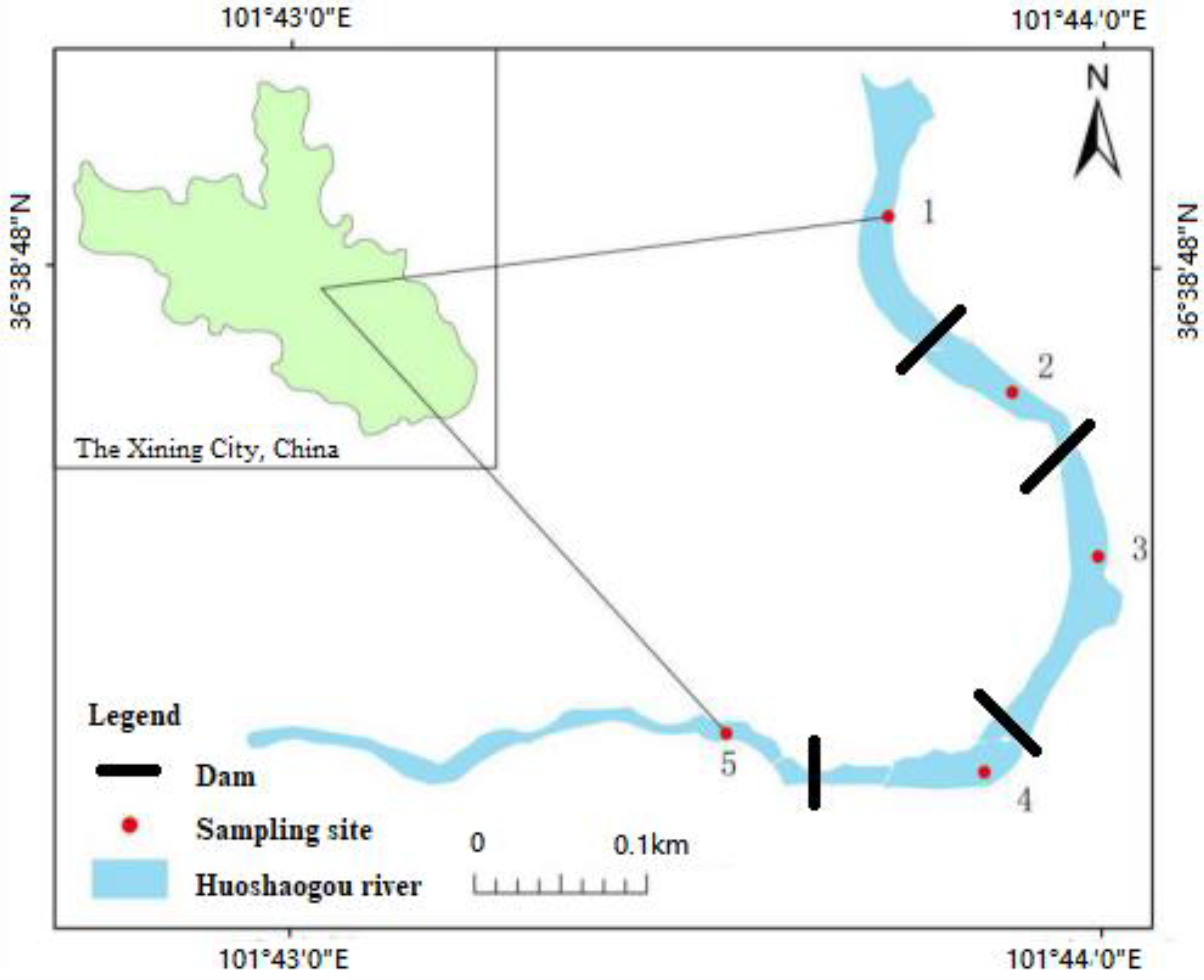
2. Study Sites
3. Data and Methods
3.1. Experimental Apparatus
3.2. Sampling Procedures
3.3. Calculation of CO2, CH4, and N2O Flux
3.4. Calculation of Variation Coefficient and Accumulative Coefficient
3.5. Influencing Factors of GHG Flux Variation and Accumulative Effect
4. Results
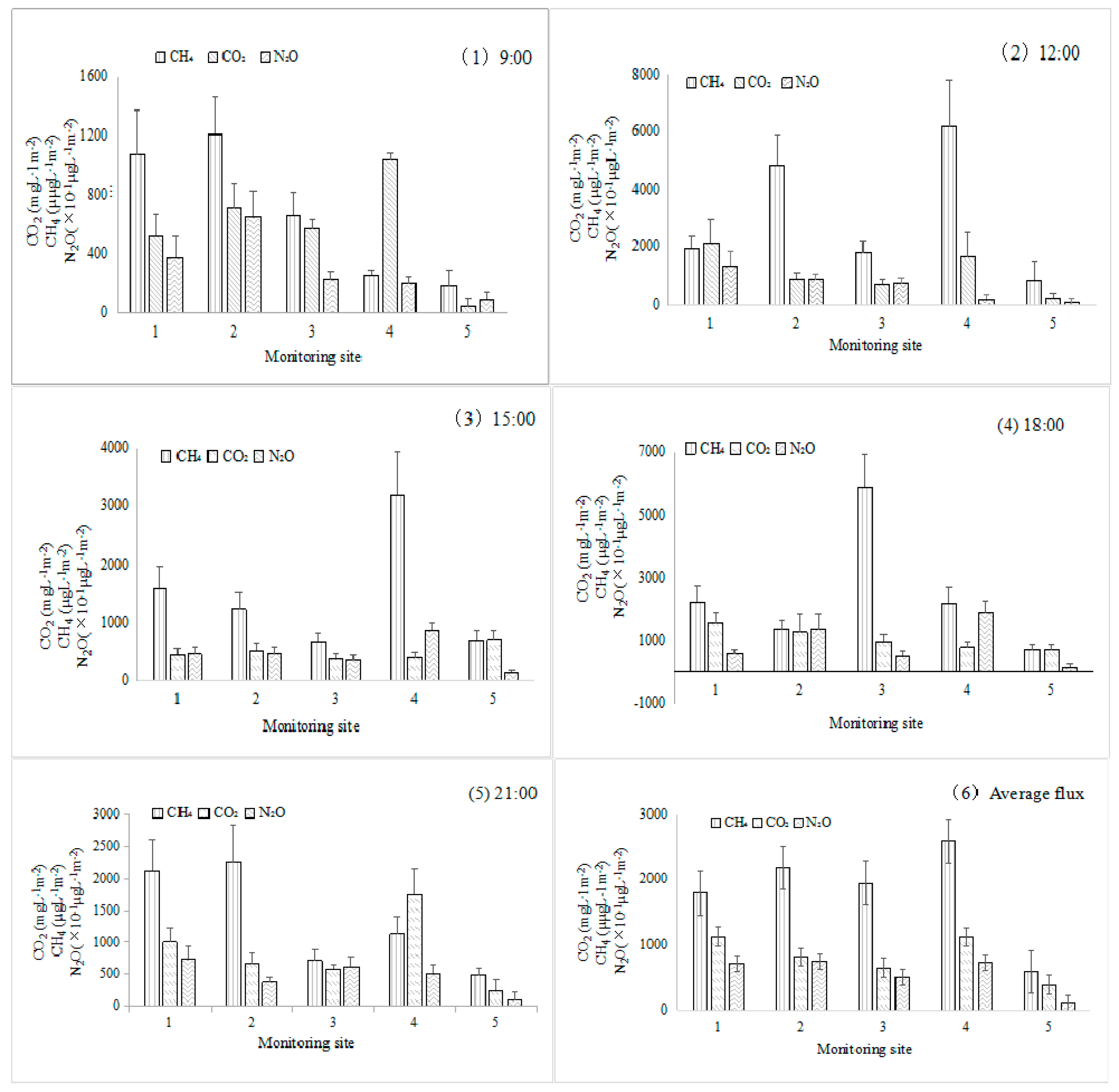
4.1. Dams Lead to a Sharply Increase in GHG Emission Flux
4.2. GHGs React More Robust to Continuous Dams than Environmental Factors
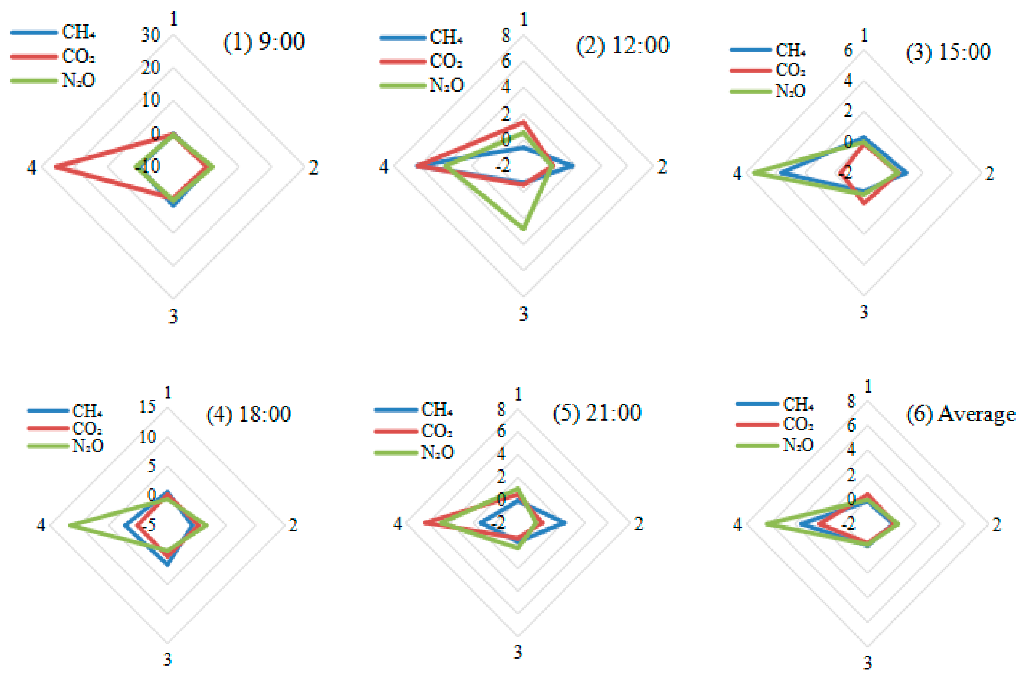
4.3. Cumulative Effect from Continuous Dam Was Detected in Some Monitoring Periods
5. Discussion
5.1. Principal Influencing Factors of GHG Emissions
5.2. Potential Influencing Factors of Accumulative Changes
6. Conclusions
Author Contributions
Funding
Acknowledgments
Conflicts of Interest
References
- Lehner, B.; Liermann, C.R.; Revenga, C.; Vörösmarty, C.; Fekete, B.; Magome, J.; Nilsson, C.; Robertson, J.C.; Rödel, R.; Sindorf, N.; et al. High-resolution mapping of the world’s reservoirs and dams for sustainable river-flow management. Front. Ecol. Environ. 2011, 9, 494–502. [Google Scholar] [CrossRef] [Green Version]
- Moran, E.F.; Lopez, M.C.; Moore, N.; Müller, N.; Hyndman, D.W. Sustainable hydropower in the 21st century. Proc. Natl. Acad. Sci. USA 2018, 115, 11891–11898. [Google Scholar] [CrossRef] [PubMed] [Green Version]
- Mosier, A.R.; Halvorson, A.D.; Reule, C.A.; Liu, X.J. Net global warming potential and GHGs intensity in irrigated cropping systems in northeastern Colorado. J. Environ. Qual. 2006, 35, 1584–1598. [Google Scholar] [CrossRef] [PubMed] [Green Version]
- Mendonça, R.F.; Kosten, S.; Sobek, S.; Barros, N.; Cole, J.J.; Tranvik, L.; Roland, F. Hydroelectric carbon sequestration. Nat. Geosci. 2012, 5, 838–840. [Google Scholar] [CrossRef]
- Kemenes, A.; Forsberg, B.R.; Melack, J.M. Methane release below a tropical hydroelectric dam. Geophys. Res. Let. 2007, 34, 1–5. [Google Scholar] [CrossRef]
- Räsänen, T.A.; Varis, O.; Scherer, L.; Kummu, M. GHGs emissions of hydropower in the Mekong River Basin. Environ. Res. Lett. 2018, 13, 034030. [Google Scholar] [CrossRef]
- Song, C.; Gardner, K.H.; Klein, S.J.W.; Souza, S.P.; Mo, V.V. Cradle-to-grave GHGs emissions from dams in the United States of America. Renew. Sust. Energ. Rev. 2018, 90, 945–956. [Google Scholar] [CrossRef] [Green Version]
- St. Louis, V.L.; Kelly, C.A.; Duchemin, É.; Rudd, J.W.M.; Rosenberg, D.M. Reservoir surfaces as sources of greenhouse gases to the atmosphere: A global estimate: Reservoirs are sources of greenhouse gases to the atmosphere, and their surface areas have increased to the point where they should be included in global inventories of anthropogenic emissions of greenhouse gases. BioScience 2000, 50, 766–775. [Google Scholar] [CrossRef]
- Andrew, R.; Balch, E.; Wollheim, W.M. Spatial Patterns of GHGs Across an Urbanization Gradient in a Suburban River Network. AGUFM 2017, H23I-1792. [Google Scholar]
- Santos, M.A.; Damazio, J.M.; Rogerio, J.P.; Amorima, M.A.; Medeiros, M.A.; Abreu, L.S.; Maceira, E.P.; Melo, A.C.; Rosa, M.P. Estimates of GHG emissions by hydroelectric reservoirs: The Brazilian case. Energy 2017, 133, 99–107. [Google Scholar] [CrossRef]
- Liikanen, A.; Murtoniemi, T.; Tanskanen, H.; Väisänen, T.; Martikainen, P.J. Effects of temperature and oxygen availability on greenhouse gas and nutrient dynamics in sediment of a eutrophic mid-boreal lake. Biogeochemistry 2002, 59, 269–286. [Google Scholar] [CrossRef]
- Liu, X.; Li, S.; Wang, Z.; Han, B.; Li, J.; Wang, F.; Bai, L. Nitrous oxide (N2O) emissions from a mesotrophic reservoir on the Wujiang River, southwest China. Acta Geochim. 2017, 36, 667–679. [Google Scholar] [CrossRef]
- Soumis, N.; Duchemin, É.; Canuel, R.; Marc, L. GHGs emissions from reservoirs of the western United States. Glob. Biogeochem. Cycles 2004, 18. [Google Scholar] [CrossRef]
- Abril, G.; Guérin, F.; Richard, S.; Robert, D.; Corinne, G.L.; Philippe, G.; Alain, T.; Louis, V.; Marco, A.D.S.; Bohdan, M. Carbon dioxide and methane emissions and the carbon budget of a 10-year old tropical reservoir (Petit Saut, French Guiana). Glob. Biogeochem. Cycles 2005, 19, 1–16. [Google Scholar] [CrossRef]
- Fearnside, P.M. Greenhouse gas emissions from a hydroelectric reservoir (Brazil’s Tucuruí Dam) and the energy policy implications. Water Air Soil Poll. 2002, 133, 69–96. [Google Scholar] [CrossRef]
- Hidrovo, A.B.; Uche, J.; Martínez-Gracia, A. Accounting for GHG net reservoir emissions of hydropower in Ecuador. Renew. Energy 2017, 112, 209–221. [Google Scholar] [CrossRef] [Green Version]
- Barros, N.; Cole, J.J.; Tranvik, L.J.; Prairie, Y.T.; Bastviken, D.; Huszar, V.L.; Roland, F. Carbon emission from hydroelectric reservoirs linked to reservoir age and latitude. Nat. Geosci. 2011, 4, 593–596. [Google Scholar] [CrossRef]
- Wang, H.; Wu, X.; Bi, N.; Li, S.; Yuan, P.; Wang, A.; Syvitski, J.P.M.; Saito, Y.; Yang, Z.S.; Liu, S.M.; et al. Impacts of the dam-orientated water-sediment regulation scheme on the lower reaches and delta of the Yellow River (Huanghe): A review . Glob. Planet. Chang. 2017, 157, 93–113. [Google Scholar] [CrossRef]
- Wu, N.; Tang, T.; Fu, X.; Jiang, W.; Li, F.; Zhou, S.; Fohrer, N. Impacts of cascade run-of-river dams on benthic diatoms in the Xiangxi River, China. Aquat. Sci. 2010, 72, 117–125. [Google Scholar] [CrossRef]
- Liu, Q.; Liu, S.; Zhao, H.; Deng, L.; Wang, C.; Zhao, Q.; Dong, S. The phosphorus speciations in the sediments up-and down-stream of cascade dams along the middle Lancang River. Chemosphere 2015, 120, 653–659. [Google Scholar] [CrossRef]
- Cocklin, C.; Parker, S.; Hay, J. Notes on cumulative environmental change I: Concepts and issues. J. Environ. Manag. 1992, 35, 31–49. [Google Scholar] [CrossRef]
- Li, J.; Dong, S.; Liu, S.; Yang, Z.; Peng, M.; Zhao, C. Effects of cascading hydropower dams on the composition, biomass and biological integrity of phytoplankton assemblages in the middle Lancang-Mekong River. Ecol. Eng. 2013, 60, 316–324. [Google Scholar] [CrossRef]
- Ouyang, W.; Hao, F.; Song, K.; Zhang, X. Cascade dam-induced hydrological disturbance and environmental impact in the upper stream of the Yellow River. Water. Res. Manag. 2011, 25, 913–927. [Google Scholar] [CrossRef]
- Matthews, C.J.; St Louis, V.L.; Hesslein, R.H. Comparison of three techniques used to measure diffusive gas exchange from sheltered aquatic surfaces. Environ. Sci. Technol. 2003, 37, 772. [Google Scholar] [CrossRef]
- Tremblay, A.; Varfalvy, L.; Garneau, M.; Roehm, C. Greenhouse Gas Emission–Fluxes and Processes: Hydroelectric Reservoirs and Natural Environments; Springer: Berlin/Heidelberg, Germany, 2005. [Google Scholar]
- Maucieri, C.; Barbera, A.C.; Vymazal, J.; Borin, M. A review on the main affecting factors of greenhouse gases emission in constructed wetlands. Agric. For. Meteorol. 2017, 236, 175–193. [Google Scholar] [CrossRef]
- Qu, B.; Aho, K.S.; Li, C.; Kang, S.; Sillanpää, M.; Yan, F.; Raymond, P.A. Greenhouse gases emissions in rivers of the Tibetan Plateau. Sci. Rep. 2017, 7, 1–8. [Google Scholar] [CrossRef] [Green Version]
- Demarty, M.; Bastien, J. GHG emissions from hydroelectric reservoirs in tropical and equatorial regions: Review of 20 years of CH4 emission measurements. Energy Policy 2011, 39, 4197–4206. [Google Scholar] [CrossRef]
- He, B.; He, J.; Wang, J.; Li, J.; Wang, F. Characteristics of GHG flux from water-air interface along a reclaimed water intake area of the Chaobai River in Shunyi, Beijing. Atmos. Environ. 2018, 172, 102–108. [Google Scholar] [CrossRef]
- Wang, F.; Wang, B.; Liu, C.Q.; Wang, Y.; Guan, J.; Liu, X.; Yu, Y. Carbon dioxide emission from surface water in cascade reservoirs–river system on the Maotiao River, southwest of China. Atmos. Environ. 2011, 45, 3827–3834. [Google Scholar] [CrossRef]
- Teodoru, C.R.; Nyoni, F.C.; Borges, A.V.; Darchambeau, F.; Nyambe, I.; Bouillon, S. Dynamics of greenhouse gases (CO2, CH4, N2O) along the Zambezi River and major tributaries, and their importance in the riverine carbon budget. Biogeosciences 2015, 12, 2431–2453. [Google Scholar] [CrossRef] [Green Version]
- Stow, C.A.; Walker, J.T.; Cardoch, L.; Spence, P.; Geron, C. N2O emissions from streams in the Neuse River watershed, North Carolina. Environ. Sci. Technol. 2005, 39, 6999–7004. [Google Scholar] [CrossRef] [PubMed]
- Maltais-Landry, G.; Maranger, R.; Brisson, J.; Chazarenc, F. Greenhouse gas production and efficiency of planted and artificially aerated constructed wetlands. Environ. Pollut. 2009, 157, 748–754. [Google Scholar] [CrossRef] [PubMed]
- Mander, Ü.; Lohmus, K.; Teiter, S.; Nurk, K.; Mauring, T.; Augustin, J. Gaseous fluxes from subsurface flow constructed wetlands for waste water treatment. J. Environ. Sci. Heal. 2005, 40, 1215–1226. [Google Scholar] [CrossRef] [PubMed]
- Thu, N.; An, P.; Amateurishness, B.; Chaos, L.; Sun, L.; Microchip, M.; Memoriam, Y. Effect of plant harvest on methane emission from two constructed wetlands designed for the treatment of rosewater. J. Environ. Manag. 2007, 85, 936–943. [Google Scholar] [CrossRef]
- Cole, J.J.; Caraco, N.F. Emissions of nitrous oxide (N2O) from a tidal, freshwater river, the Hudson River, New York. Environ. Sci. Technol. 2001, 35, 991–996. [Google Scholar] [CrossRef]
- Deemer, B.R.; Harrison, J.A.; Whitling, E.W. Microbial dinitrogen and nitrous oxide production in a small eutrophic reservoir: An in situ approach to quantifying hypolimnetic process rates. Limnol. Oceanogr. 2011, 56, 1189–1199. [Google Scholar] [CrossRef]
- Milton, M.H.; Morell, J.M.; Corredor, J.E. Increase of nitrous oxide flux to the atmosphere upon nitrogen addition to red mangroves sediments. Mar. Pollut. Bull. 2002, 44, 992–996. [Google Scholar] [CrossRef]
- Dijkstra, F.A.; Prior, S.A.; Runion, G.B.; Torbert, H.A.; Tian, H.; Lu, C.; Venterea, R.T. Effects of elevated carbon dioxide and increased temperatureon methane and nitrous oxide fluxes: Evidence from field experiments. Front. Ecol. Environ. 2012, 10, 520–527. [Google Scholar] [CrossRef]
- Gagnon, L.; Van de Vate, J.F. Greenhouse gas emissions from hydropower: The state of research in 1996. Energy Policy 1997, 25, 7–13. [Google Scholar] [CrossRef]
- Prusty, S.; Mohini, M.; Kundu, S.S.; Kumar, A.; Datt, C. Methane emissions from river buffaloes fed on green fodders in relation to the nutriet intake and digestibility. Trop. Anim. Health Prod. 2014, 46, 65–70. [Google Scholar] [CrossRef]
- Tremblay, A.; Therrien, J.; Hamlin, B.; Wichmann, E.; LeDrew, L.J. GHG emissions from boreal reservoirs and natural aquatic ecosystems. In Greenhouse Gas Emissions—Fluxes and Processes; Springer: Berlin/Heidelberg, Germany, 2005; pp. 209–232. [Google Scholar]
- Whitman, W.B. Microbial Production and Consumption of Greenhouse Gases: Methane, Nitrogen Oxides, and Halomethanes; Rogers, J.E., Ed.; American Society for Microbiology: Washington, DC, USA, 1991; pp. 39–55. [Google Scholar]
- Haggard, B.E.; Storm, D.E.; Stanley, E.H. Effect of a point source input on stream nutrient retention. J. Am. Water Resour. Assoc. 2006, 37, 1291–1299. [Google Scholar] [CrossRef]


| Indicators | Secondary Indicator | Summer | Autumn | Average |
|---|---|---|---|---|
| Hydrology | pH | 0.98 | 1.21 | 1.095 |
| DO | 0.76 | 0.72 | 0.74 | |
| Water temperature | 1.04 | 1.09 | 1.06 | |
| Conductivity | 0.91 | 0.89 | 0.90 | |
| Water quality | TN | 1.24 | 1.16 | 1.70 |
| TP | 1.07 | 1.87 | 1.47 | |
| TOC | 1.42 | 1.57 | 1.49 | |
| CODmn | 1.43 | 1.29 | 1.36 | |
| Vegetation | TN | 2.03 | 2.19 | 2.11 |
| TP | 1.53 | 1.93 | 1.73 | |
| TOC | 1.74 | 1.95 | 1.84 | |
| Sediments | TN | 1.49 | 1.39 | 1.44 |
| TP | 2.05 | 1.85 | 1.95 | |
| TOC | 2.07 | 2.03 | 2.05 | |
| GHGs | CO2 | 4.6 | 2.96 | 3.78 |
| CH4 | 5.82 | 3.37 | 4.59 | |
| N2O | 8.44 | 5.01 | 6.72 |
| No. | Influenceing Indicator | Principal Component | ||||
|---|---|---|---|---|---|---|
| 1 | 2 | 3 | 4 | 5 | ||
| 1 | Light intensity | 0.120 | 0.007 | 0.175 | 0.250 | 0.856 |
| 2 | Wind speed | 0.591 | −0.027 | 0.205 | −0.010 | −0.500 |
| 3 | Water temperature | 0.637 | 0.114 | 0.651 | −0.179 | −0.055 |
| 4 | Air Temperature | 0.665 | 0.157 | 0.504 | −0.008 | 0.080 |
| 5 | DO | −0.099 | −0.327 | −0.412 | 0.397 | 0.095 |
| 6 | EC | 0.708 | −0.314 | −0.495 | 0.276 | 0.007 |
| 7 | ORP | −0.787 | −0.103 | −0.417 | 0.074 | −0.048 |
| 8 | pH | 0.737 | 0.238 | −0.218 | −0.045 | −0.349 |
| 9 | Salinity | 0.566 | −0.124 | 0.360 | −0.066 | 0.382 |
| 10 | TDS | 0.718 | −0.293 | −0.503 | 0.235 | 0.026 |
| 11 | TOC (vegetation) | −0.026 | 0.883 | −0.182 | 0.170 | −0.008 |
| 12 | N (vegetation) | 0.081 | 0.903 | −0.070 | 0.417 | −0.007 |
| 13 | P (plant) | 0.465 | 0.617 | −0.262 | 0.442 | 0.074 |
| 14 | TN (sediment) | −0.310 | −0.138 | 0.523 | 0.748 | −0.189 |
| 15 | TP (sediment) | −0.477 | 0.667 | 0.014 | −0.450 | 0.081 |
| 16 | TOC (sediment) | −0.513 | −0.143 | 0.586 | 0.569 | −0.196 |
| No. | Influencing Indicator | GHGs | ||
|---|---|---|---|---|
| CO2 | CH4 | N2O | ||
| 1 | Light intensity | −0.124 | −0.153 | 0.393 * |
| 2 | DO | 0.147 | 0.099 | −0.332 * |
| 3 | EC | 0.305 | −0.300 | 0.249 |
| 4 | ORP | −0.383 * | 0.380 | 0.213 |
| 5 | pH | −0.303 | −0.333 * | 0.090 |
| 6 | Salinity | −0.401 | −0.341 | −0.252 |
| 7 | Wind speed | 0.409 | −0.097 | −0.531 ** |
| 8 | Water temperature | 0.612 ** | 0.609 ** | 0.012 |
| 9 | Air Temperature | 0.142 | 0.309 * | 0.113 |
| 10 | TDS | −0.132 | 0.315 | 0.018 |
| 11 | TOC (plant) | 0.441 ** | 0.141 | −0.252 |
| 12 | N (plant) | 0.309 | −0.097 | −0.531 ** |
| 13 | P (plant) | 0.012 | −0.014 | 0.212 |
| 14 | TN (sediment) | −0.153 | −0.047 | 0.513 ** |
| 15 | TP (sediment) | −0.099 | −0.214 | 0.018 |
| 16 | TOC (sediment) | 0.334 * | 0.713 ** | 0.013 |
© 2020 by the authors. Licensee MDPI, Basel, Switzerland. This article is an open access article distributed under the terms and conditions of the Creative Commons Attribution (CC BY) license (http://creativecommons.org/licenses/by/4.0/).
Share and Cite
Yang, D.; Mao, X.; Wei, X.; Tao, Y.; Zhang, Z.; Ma, J. Water–Air Interface Greenhouse Gas Emissions (CO2, CH4, and N2O) Emissions Were Amplified by Continuous Dams in an Urban River in Qinghai–Tibet Plateau, China. Water 2020, 12, 759. https://doi.org/10.3390/w12030759
Yang D, Mao X, Wei X, Tao Y, Zhang Z, Ma J. Water–Air Interface Greenhouse Gas Emissions (CO2, CH4, and N2O) Emissions Were Amplified by Continuous Dams in an Urban River in Qinghai–Tibet Plateau, China. Water. 2020; 12(3):759. https://doi.org/10.3390/w12030759
Chicago/Turabian StyleYang, Dengxing, Xufeng Mao, Xiaoyan Wei, Yaqing Tao, Zhifa Zhang, and Jianhai Ma. 2020. "Water–Air Interface Greenhouse Gas Emissions (CO2, CH4, and N2O) Emissions Were Amplified by Continuous Dams in an Urban River in Qinghai–Tibet Plateau, China" Water 12, no. 3: 759. https://doi.org/10.3390/w12030759