Nonlinear Dynamic Modeling of Urban Water Consumption Using Chaotic Approach (Case Study: City of Kelowna)

Abstract

This study investigated urban water consumption complexity using chaos theory to improve forecasting performance to help optimize system management, reduce costs and improve reliability. The objectives of this study were to (1) investigate urban water distribution consumption complexity and its role in forecasting technique performance, (2) evaluate forecasting models by periodicity and lead time, and (3) propose a suitable forecasting technique based on operator applications and performance through various time scales. An urban consumption dataset obtained from the City of Kelowna (British Columbia, Canada) was used as a test case to forecast future consumption values using varying lead times under different temporal scales to identify models which may improve forecasting performance. Chaos theory techniques were employed to inform model optimization. This study attempted to address the paucity of studies on chaos theory applications in water consumption forecasting. This was accomplished by applying non-linear approximation, dynamic investigation, and phase space reconstruction for input variables, to improve the accuracy in various periodicity and lead time. To reconstruct the phase space, lag time was calculated using average mutual information for daily resolution as 17 days to reconstruct the phase space. The optimum embedding dimension and correlation exponent for the phase space were 18 and 3.5, respectively. Comparing the results, the non-linear local approximation model provided the best performance. The forecasting horizon for the models was 122 days. Moreover, phase space reconstruction improved the accuracy of the models for the different lead times. The findings of this study may improve forecasting performance and provide evidence to support further investigation of the chaotic behaviour of water consumption values over different time scales.

1. Introduction

Global water scarcity concerns are increasing due to climate change, urban development, population growth, industrial development, economic expansion, and the cost of drinking water [1]. It is imperative that governments invest in integrated management plans that address consequences of water problems such as scarcity of available water resources, sufficient distribution and pipeline maintenance. Conflicts resulting from water scarcity are becoming more prevalent and severe than other natural resource scarcity due to rapid increases in population without access to reliable sources of fresh water in recent decades [1,2]. There were 153 water-related conflicts reported in the 19th century while 279 conflicts have been reported within the last decade [3]. Therefore, we highlight the necessity of a management plan that improves water consumption efficiency.

A robust operation of urban drinking water supply systems requires future water consumption values to inform the development of an efficient water consumption management plan to mitigate anticipated stressors on the system. The reliability of water distribution systems may be improved through the accurate simulation of hydraulic conditions in pipeline systems based on future water consumption forecasting. In other words, water consumption forecasting provides public suppliers with the necessary future consumption information to ensure consumption needs can be met [4,5]. Water consumption forecasting is a dynamic process as predictions are essential for the optimum operation and sustainable growth and development of urban water supply [6]. The reason for categorizing water consumption forecasting as a dynamic process is because of the influential variables in forecasting that are not stable and can change under varying conditions. Therefore, considering reliable forecasting horizon can be beneficial in any management plan. Moreover, forecasting consumption values in short-, mid-, and long-term (i.e., less than a week, a week to a month, a month to a year or more, respectively) time periods play a crucial role in water distribution systems’ (WDS) daily operation basis by informing important factors such as optimized pumping, pipeline maintenance, minimizing energy and water supply cost, improving system reliability and the quality of allocated water [7,8,9]. Recent studies have improved the understanding of the nonlinearity and complexity of water consumption factors; however, more study on these concepts is required. The available studies related to these factors are limited and require (1) accurate estimation and forecasting of water consumption and (2) determination of the degree of nonlinearity among the influential variables in water consumption. Accurate estimation and forecasting data are influenced by the availability of high-resolution temporal scale datasets (e.g., daily and hourly). Additionally, data availability for other influential factors, such as holidays, humidity, peak consumption duration in a 24-h period, air temperature, population growth, and consumers’ income, is important to accurately forecast consumption data.

Over the past three decades, two thoughts of deterministic and probabilistic methods have been proposed to forecast urban water consumption. The deterministic approach is solely based on input variables and their initial conditions, whereas a probabilistic model relies on modeling uncertainties and randomness of input variables. Researchers have confirmed the ability of nonlinear deterministic approaches in modeling the events with complexity in effective variables [10,11]. Individual consumption habits are an important factor in modeling and forecasting future consumption. However, there are a few studies that aimed to forecast water consumption at the individual household scale which is a technique to analyze consumption habits [12]. The authors are not aware of any recent studies that considered consumers’ habits in total recorded consumption values when modeling urban water consumption in large scale of an urban district.

However, an individual’s habits will influence consumption and thus, future values in the system will be highly influenced by individual consumer habits, resulting in a highly complex system. In a complex system, “the behavior of the integral part of the system is simple, but the behavior of the overall system is complex” [13]. Given the significant challenges and complexity of probabilistic methods, deterministic methods can provide a useful approximation to their probabilistic counterparts. Therefore, investigation of the complexity of effective variables that are used as input variables of water consumption models can provide information towards employing a reliable modeling technique. Therefore, this study investigates both the dynamic characteristics, and dynamic explanatory variables in water consumption within the City of Kelowna (British Columbia, Canada). Furthermore, this research focuses on a deterministic approach to forecast short-term and mid-term lead times under different temporal scales. To calibrate the forecasting models, urban dimension of the test data is considered (i.e., the whole urban scale, rather than neighborhoods or single buildings). This decision may have implications on usability of the model information for consumption and supply management.

1.1. Background

Information about future water consumption helps related authorities develop an integrated, efficient plan that reduces long-term supplier and consumer water stress. Accurate estimation of drinking water consumption and availability of resources is considered one of the solutions to reduce water stress [9,14,15,16]. Moreover, having an accurate estimation of future consumption values improves sustainability for planning purposes. Unlike forecasting for other water resources-related parameters of interest (e.g., river discharge, sedimentation, rainfall, etc.), where influential factors in forecasting the goal values are mostly correlated (e.g., rainfall factors in modeling and simulating of river discharge), influential variables in forecasting water consumption are more complex with a weaker correlation. Moreover, applying large datasets with many input variables can lead to overfitting issues, which can misrepresent model performance through overly confident forecasting model predictions in addition to adding model complexity without improving accuracy. Hence, consumption forecasting requires a balance of optimizing the quantity of input variables with improvements in forecasting accuracy. It can improve the accuracy of the models while reducing the number of input variables by defining the model’s input with active variables. Input variable selection techniques (e.g., Garson Equation, Influential correlation) are employed to highlight the active variables in a system [17].

There are different types of variables affecting consumption values such as climatic (e.g., temperature, relative humidity, rainfall, etc.) and socioeconomic (e.g., population and income) [18]. Commonly climatic variables are used in short-term and mid-term forecasting while socioeconomic variables are used to forecast long-term consumption values [19,20,21]. Common climatic factors considered in recent studies are temperature, precipitation, and previously recorded consumption values [20,22,23]. The number of studies on short- and mid-term forecasting of water consumption is considerable; however, limited studies have specifically investigated impact of climatic factors on consumption forecasting in the same period [24,25,26].

The literature enlists implementation of different statistical and probabilistic approaches for forecasting consumption values. Generally, conventional techniques were reportedly prevalent for a better understanding of chosen variables in the modeling of water consumption [27,28,29], which consider linear relationships between functional variables and the value of water consumption, while observation indicates that these relationships exhibit nonlinear behavior. The literature is mostly categorized into physical-based and black box models. Physical-based models approximate the general internal sub-process and physical mechanism by fundamental laws of mass, energy, and momentum. Black box models implement artificial intelligence, fuzzy based and nonlinear deterministic methods (e.g., artificial neural networks, genetic programming, support vector machine, nonlinear local approximation, etc.) to ascertain the relationship between the input and output variables. The physical-based and black box models include conventional regression models [9], artificial neural networks (ANN) [14,20,30,31], feedforward neural networks (FNN) [22,32], general regression neural networks (GRNNs) [33,34], deep belief neural network (DBNN) [35], support vector machines (SVMs) [16,18,36,37,38], gene expression programming (GEP) [39,40], adaptive neural fuzzy inference system (ANFIS) [41], Fourier analysis [7], hybrid models (e.g., combined wavelet) [23,42,43], fuzzy regression [44], fuzzy cognitive map learning method [45], epidemiology-based forecasting framework [46], temporal disaggregation [47], harmonic analysis [48], and wavelet de-noising [49].

Influential factors in complex water consumption systems may benefit from chaos theory techniques to improve forecasting methods. As mentioned above, characteristics of influential factors in water consumption are characterized as complex systems. Chaos theory techniques may improve the application of forecasting models to estimate future values in complex systems and improve the prediction of nonlinearity within dynamic systems [13,50]. Descriptions of chaotic behavior have been used in various engineering applications. Chaotic systems are defined and characterized by large changes in behavior resulting from small changes in initial conditions of the system [51]. Using the ‘extent of complexity’ of a chaotic system (defined primarily in the context of the variability of relevant data), chaotic systems are classified as low-, medium- or high-dimensional [52]. Moreover, the availability of noise in time series increases the complexity of the data and results in a high embedding dimension [53]. In water distribution systems, factors such as temperature, humidity, precipitation, the economic condition of consumers, population size, holidays, etc., have an impact on water consumption. By aggregating data at increasing temporal scales, the effects of scaling time series on deterministic chaos can be found [54,55] and any missing data can be generated [56,57]. This approach has been used in solving problems in various fields of study such as river discharge [58,59,60], sedimentation [61,62,63], climate [64], lake level variability [65,66], rainfall [67,68,69,70], traffic speed [71], finance [72], image processing [73] and ship motion prediction [74]. However, there is a paucity of study on the application of chaos theory on water consumption forecasting methods. Oshima [13] developed a real-time forecasting system for water consumption based on the chaos theory. To support operations with labor saving, facility maintenance and efficient use of energy, he introduced “information integration type chaos theory-based consumption forecasting”. The report showed the application of chaos-based techniques in improving the accuracy of the results.

Evolutionary techniques became popular in modeling and optimizing fields. Genetic programming (GP) and gene expression programming (GEP) place on heuristic algorithms that are found in Darwin’s evolution theory [66]. Evolutionary techniques adjust the population of a specific solution. In each stage, individuals are selected randomly from the current population. Then, the chosen individual plays the parent’s role to be reproduced for another population for the next generation of solutions. This reproduction goes toward an optimal answer which has been defined as the goal values. The evolutionary techniques are used for optimization problems where standard methods are not suitable, such as discontinuity, nondifferentiable, stochastic, or highly nonlinear objective functions. Among evolutionary techniques, GP and GEP are used for modeling problems with the same abilities as GA such as informing data gaps and forecasting time series [18,75,76,77]. Aytek and Kishi [78] used the GP technique to model suspended sediment load in the Tongue River (United States) and reported better performance from GP compared to sediment rating curves and multiple linear regressions (MLR). Since GEP provides a tree-structure scheme, it makes GEP more convenient to interpret the results in comparison with GP. Moreover, GEP presents mathematical equations that clarify the relationship between input and output variables by a factor of 100-10000 [63,79,80]. The superiority of GEP and the advantages of this technique interested researchers to develop more sophisticated models with hybrid methods such as combining the extended Kalman filter [81], clustering the consumption values [82], Wavelet decomposition [39], and phase space reconstructed GEP (PSR-GEP) [42] in forecasting urban drinking water consumption. The results showed that GEP models are highly sensitive to wavelet decomposition when attempting to improve the performance of the models.

1.2. Problem Statement

Growth in peak water consumption, which overburdens urban water resources [30], requires an efficient management plan. This importance motivated the application of soft-computing techniques into urban water consumption forecasting methods to develop methods that are applicable in forecasting problems. Many techniques have been proposed to forecast water consumption under differing time scales; however, there has been limited investigation on performance comparisons between models to inform model selection under various conditions [5]. Moreover, non-stationary, non-linear, and inherent stochasticity of water consumption data makes forecasting problems more challenging in this field [83]. Donkor et al. [84] reported that periodicity and forecasting horizon influence the performance of the methods in short-term and long-term forecasting, such as artificial neural networks and econometric models, respectively. Therefore, understanding the forecasting horizon, which is dependent on the dataset considered, will help to categorize the performance of the developed models. It can be considered as a classification for short-, mid-, and long-term forecasting models, which help operators select the appropriate model to implement considering the available dataset [9,20,85]. Forecasting horizon can improve the reliability of consumption forecasting methods by informing which method is most useful for consumption forecasting under specified time frames; however, in general, there is currently no acknowledgement of time frame for these forecasting horizons [84]. This study focuses on the forecasting horizon for the considered models to inform performance under various periodicity (daily, 2-day, 4-day, weekly, bi-weekly, and monthly) and lead time.

Based on previous studies, common influential variables in water consumption forecasting include observed consumption values (e.g., historical recorded consumption values over various periodicity), climatic variables (e.g., temperature, humidity, levels of snow and rainfall) and socioeconomic variables (e.g., population growth rate, economic factors such as income and water cost) [5]. Although these variables are used in the literature, there are fewer studies that used socioeconomic variables in long-term forecasting than studies that employed the above-mentioned variables. Moreover, extrapolation models in water consumption forecasting are based on the recorded data and its error terms [84]. The limitation of these models is based on their dependence of past trends that will likely be observed in the future, but do not consider the role socioeconomic variables and consumer habits may play in influencing future consumption values. Recently published studies investigating these factors are limited and require (1) accurate estimation and forecasting of water consumption considering different periodicity and forecasting horizons to classify the models based on their performance, and (2) determination of the degree of nonlinearity among the influential variables to consider exogenous variables (e.g., socioeconomic). The role of these factors in the value of water consumption in the future is highlighted. Therefore, investigating the complexity of input data can be helpful in employing different techniques with various abilities to model forecasting water consumption problems.

1.3. Objective

The techniques presented in the literature are often considered for short-term forecasting, which is based on one-day-ahead lead time. In light of the previous discussion on model limitations, it has been reported that the weaknesses of the forecasting models are related to the lack of consideration for the complex behavior of water consumption datasets. Much of the existing research ignores the importance of dynamic behavior of consumption datasets although many pre-processing techniques have been introduced to improve model accuracy. This study investigates the dynamics of a dataset to detect chaotic behavior of water consumption time series. Then, a non-linear approximation technique is applied to forecast water demand consumption. The objective of this study was to (1) investigate system complexity and its role in forecasting technique performance, (2) evaluate selected forecasting models by periodicity and lead time, and (3) propose a suitable forecasting technique based on operator applications and performance through different time scales.

This study improves the understanding of nonlinear local approximation (NLA) performance in comparison with previously introduced methods in water consumption forecasting. Moreover, forecasting horizon is introduced as a factor to evaluate the performance of forecasting models. This study attempts to address gaps in previous studies by applying NLA, dynamic investigation, phase space reconstruction for input variables, and improving the accuracy in various periodicity and lead times.

2. Materials and Methods

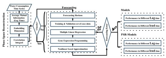
Figure 1 provides a schematic description of the research methodology. Average mutual information (AMI) is used to calculate the lag time. Then, the existence of chaotic behavior in the test case is investigated by the correlation dimension method. Four different methods are employed to forecast the short- and mid-term consumption values. Non-Linear local approximation method is considered as the forecasting method in the condition of the test data that has chaotic behavior. The performance of selected models is evaluated in different lag and lead times.

2.1. Phase Space Reconstruction

This research employed the phase-space concept to better understand the dynamic nature of a municipal water consumption dataset for the City of Kelowna. The dynamics of a water consumption system are represented by data points along a trajectory, whereby each position in time represents a system state. The lag-embedding technique can be used on deterministic, dynamic systems such as the present water consumption dataset to reconstruct phase-space from time series. The fundamental dynamics of a system can be studied by reconstructing an m-dimensional phase-space of Dt that is defined by [86,87]:

$$D_t=\left\{d_t,d_{t-\tau },d_{t-2\tau },\dots ,d_{t-\left(m-1\right)\tau }\right\},t=1,2,3,\dots ,N$$

(1)

where D_t is a vector of the consumption data of {d_t}_t=1,…,N, N is the number of recorded consumption data points, $\tau$ is the lag time and m is the number of embedding dimension that generally varies from 1 to 10 or 1 to 20 [61,66,88,89]. In the case when m is greater than the minimum embedding dimension, the trajectory of reconstructed vectors can display the true state of the chaotic system. Indeed, the lag time ($\tau$) is arbitrary as the data are often assumed to have infinite precision. The lag time should not be too small given the difference between various elements of the delay vectors and, it should not be too large as this can result in low coordinate correlation [90]. If the dynamics of the system can be reduced to a set of deterministic laws, trajectories will converge towards a subset of the phase-space with a fractional dimension called the attractor [89]. The lag-embedding method is sensitive to both embedding parameters of $\tau$ and m. Average mutual information (AMI) is a well-known method for estimating the lag time [91,92]. This research employed AMI to estimate the lag time [91]:

$$I\left(d_t,d_{t+\tau }\right)={\displaystyle \sum _{d_t}\sum _{d_{t+\tau }}}P(d_t,d_{t+\tau }){\log }_2\frac{P\left(d_t,d_{t+\tau }\right)}{P\left(d_t\right)P\left(d_{t+\tau }\right)}$$

(2)

where the sum is extended over the total number of samples in the time series, P(d_t) and P(d_t+τ) are the marginal probabilities for measurements d_t and d_t+τ and P (d_t, d_t+τ) is their joint probability. The optimal τ minimizes the value of the function I (d_t, d_t+τ) for t = τ. AMI considers the first local minimum as the lag time [91,93].

2.2. Correlation Dimension

The dimension of a system informs its complexity and indicates the number of required variables that specify a deterministic system. Kermani [59] classified different dimensions in a system including topological, Hausdorf, box counting, point-wise, and correlation dimensions. Additionally, the correlation dimension is used as an indicator of a deterministic or stochastic process [59,94]. The function below calculates the correlation integral value [95]:

$$C_m\left(r\right)=\frac{2}{N\left(N-1\right)}{\displaystyle \sum _{j=1}^N\sum _{i=1}^N}H\left(r-\Vert X_i-X_j\Vert \right)$$

(3)

where N is the number of data points, H is the Heaviside step function (H (u) = 1 for u > 0, H (u) = 0 for u ≤ 0 and $u=r-\Vert X_i-X_j\Vert$, X_i is the ith state vector, and r is the radius of a sphere with the content of X_i or X_j as the center. C_m(r) is proportional to r for stochastic time series, whereas for chaotic time series, it scales with r as

$$C_m\left(r\right)\propto r^{c_e}$$

(4)

where $c_e$ is the correlation exponent defined by approximating the slope of $\log C_m\left(r\right)$ versus $\log \left(r\right)$ in logarithmic scale. If the calculated $c_e$ is unchanged by increasing the number of embedding dimensions, C_e can be considered as the correlation dimension of the attractor in the system. But, if $c_e$ is not stable as a function of embedding dimensions, this system can be considered non-chaotic [54,96,97].

2.3. Nonlinear Local Approximation

Nonlinear local approximation (NLA) can forecast a system’s future without development of an analytical model [51]. This research applied NLA to (1) test the chaotic nature of consumption data and (2) forecast the consumption in the case study. This was done by reconstructing the phase space of the dataset. It is critical in a chaos analysis to reconstruct the multi-dimensional phase space that provides a conceptual pattern for the time series. The presence of attractors in phase space indicates the possibility of chaos in the dataset. A phase-space reconstruction in a dimension m facilitates an interpretation of the underlying dynamics in the form of an m-dimensional map, f_T, by

$$X_{j+T}=f_T\left(X_j\right)$$

(5)

where X_j is the vector of dimension m at the current state of the system at time j and X_j+T is the vector of dimension m at the future state of the system at time j + T. NLA entails the subdivision of the f_T domain into many subsets. In other words, the dynamics of the system were described step-by-step locally in the phase-space [98]. In an m-dimensional space, estimating the change of trajectory with time would lead to forecasting. Considering the relation between two states ${\overrightarrow{X}}_t$ and ${\overrightarrow{X}}_{t+p}$, the behaviour at a future time (p) on the attractor was forecasted by the mapping $\overrightarrow{F}$ as [66]:

$${\overrightarrow{X}}_{t+p}\cong \overrightarrow{F}\left({\overrightarrow{X}}_t\right)$$

(6)

where the evolving dynamic of state ${\overrightarrow{X}}_t$ is influenced by nearby states. The future state ${\overrightarrow{X}}_{t+p}$ was determined by the first-order polynomial mapping $\overrightarrow{f}$ [99]:

$${\overrightarrow{X}}_{t+p}\cong \overrightarrow{F}\left({\overrightarrow{X}}_t\right)=\overrightarrow{a}+\overrightarrow{f}({\overrightarrow{X}}_t,{\overrightarrow{X}}_{t-\tau },\dots ,{\overrightarrow{X}}_{t-\left(m-1\right)\tau })$$

(7)

While the mapping $\overrightarrow{f}$ is linear, the forecasted value is nonlinear [100]. This is because every state on the trajectory belongs to a different subset defined by different expressions for $\overrightarrow{F}$.

2.4. Largest Lyapunov Exponent

The rate of convergence or divergence in different dimensions is measured using the Lyapunov exponent. A deterministic system contains at least one positive Lyapunov exponent [101]. This research employed the approach proposed by Rosenstein et al. [101] to extract the value of Lyapunov exponent for the test case. After reconstruction of phase-space, a point Y_n0 was selected and all the points in the neighborhood of Y_n, with the closer distance of r to that point were found. r is the radius of a sphere with the content of Y_n as the center. The procedure was repeated for N points in the route to find a stretch factor S:

$$S=\frac{1}{N}{\displaystyle \sum _{n_0=1}^N}\ln \left[\frac{1}{\left|u_{Y_{n0}}\right|}\sum \left|Y_{n0}-Y_n\right|\right]$$

(8)

where $\left|u_{Y_{n0}}\right|$ is the number of neighbors to point Y_n0. The plot of S verses N consists of linear and nonlinear components. The literature provides two methods for calculating the largest Lyapunov exponent (λ_max). Shang et al. [102] determined λ_max as the slope of the linear part of the curve, while Rosenstein et al. [101] determined λ_max as the average of the slope of the first part and that of the second part [89,102]. This research applied the second approach to study different temporal scales. The prediction horizon (Δt) is a time in which the consumption dataset sustains its dynamics in the most accurate forecasting; Δt was obtained as the inverse of the largest Lyapunov exponent:

$$\Delta t=\frac{1}{{\lambda }_{max}}$$

(9)

2.5. Gene Expression Programming

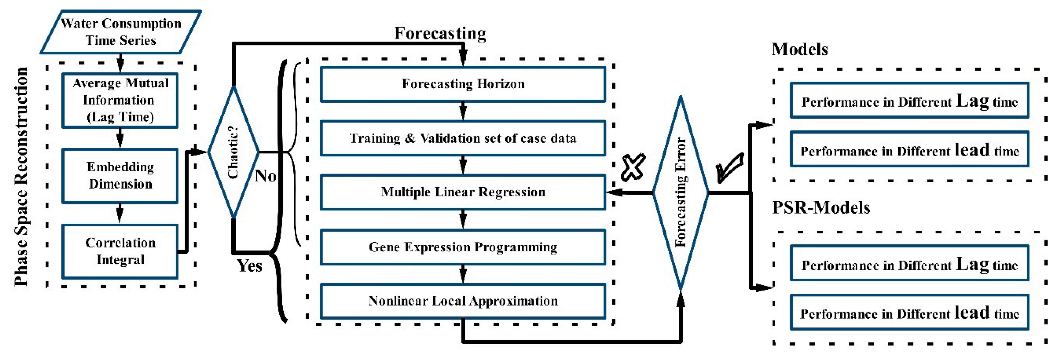
Evolutionary soft computing techniques may be applied to solve engineering problems. Among these evolutionary techniques, genetic algorithm (GA), genetic programming (GP), and gene expression programming (GEP) are considered, which were originally inspired from Darwin’s theory of evolution [79,80,103,104]. GA and GP work with a string of numbers and a specific length that is known as a “chromosome.” GEP defines an equation that shows the relationship between input and output values. Moreover, the process of the algorithm’s learning starts with the generation of chromosomes for a given random raw dataset that works with chromosomes and expression trees. Expression trees demonstrate the relationship among variables connecting with arithmetic operators. Chromosomes contain genes that provide a series of symbols of two parts, head and tail, which have functions, terminals, and only terminals, respectively. GEP follows the genome restructuring process by mutation, recombination, transposition, and gene duplication randomly. This random reputation will deliver the best model to be selected. This cycle will be continued by the reproduction of randomly generated chromosomes to reach the model with satisfying results based on defined evaluation criteria. In this research, 30 chromosomes with the head size of 8 and 3 genes are reproduced with the linking functions of $\left\{+,-,\times ,x,x^2,\sqrt{x},\log x\right\}$. The fitness functions used as the selection criteria are root mean square error (RMSE), correlation coefficient (CC) and mean absolute error (MAE). All models were selected with a fair assessment by considering stopping condition of 5000 generations. Figure 2 shows the scheme of the process with GEP method.

2.6. Multiple Linear Regression

The common application of the linear regression (LR) modeling method is to model the goal variable (Y) with a single input variable (X). Multiple linear regression (MLR) describes the relationship between the goal value (Y) and the number of input variables (X₁, X₂, …, X_n). In other words, MLR finds a relationship with a linear combination of independent explanatory variables (e.g., reconstructed phase space with a different number of embedding dimensions for recorded values of water consumption) and response variable (time ahead values of water consumption) by

$$Y_i={\alpha }_0+{\alpha }_1{X}_{i1}+{\alpha }_2{X}_{i2}+\cdots +{\alpha }_p{X}_{ip}+ϵ$$

(10)

For i = n recorded values. Y_i is the output consumption value, X_i is the explanatory input variables, dependent upon the number of embedding dimensions, where ${\alpha }_0$ is constant, ${\alpha }_p$ are slope coefficients for each input variables and $ϵ$ is the unexplained residual value.

2.7. Models Selection Criteria

Correlation Coefficient (CC), root mean square error (RMSE) and mean absolute error (MAE) are fitness functions considered in this study to evaluate model performance and accuracy.

$$\mathrm{CC}=\frac{{\sum }_{i=1}^{N_t}\left(R_i-\overline{R}\right)\left(F_i-\overline{F}\right)}{\sqrt{{\sum }_i^{N_t}{\left(R_i-\overline{R}\right)}^2}\sqrt{{\sum }_i^{N_t}{\left(F_i-\overline{F}\right)}^2}}$$

(11)

$$RMSE=\sqrt{\frac{{\sum }_{i=1}^{N_t}{\left(R_i-F_i\right)}^2}{N_t}}$$

(12)

$$MAE=\frac{1}{n}\sum _{i=1}^n\left|R_i-F_i\right|$$

(13)

Variables in the above equations include the number of values, N_t, and the recorded and forecasted values, R and F, respectively. $\overline{R}$ and $\overline{F}$ are the mean values of the recorded and forecasted water consumption, respectively. The range of CC is −1 and 1, where larger positive value of CC and smaller value for RMSE and MAE indicates better model performance in forecasting accuracy.

2.8. Test Case

Water consumption data from the City of Kelowna (British Columbia, Canada) were considered as a test case for this study. The water supply for the region comes from various resources, which include Lake Okanagan, Mission Creek, Mill Creek, Scotty Creek, Hydraulic Creek and numerous wells [105]. There is one primary distribution system that services 99% of the population via Poplar Point, Eldorado (seasonal intake uses only utilized during peak consumption) and Cedar Creek pump stations [105] plus Swick road pump station which services approximately 300 residents. This study considered Poplar Point, Eldorado and Cedar Creek stations. The SCADA system obtains information remotely from sensors installed at the intake locations. The software platform facilitates tracking of historical system performance for auditing and future decision making to optimize the system [105]. This study used six temporal scales of the consumption, including daily, 2-, 4-, 7-, 14- and 30 days from 1st of January 2010 to 30th December 2016. The test data are the whole scale of consumption values as the spatial scale for City of Kelowna.

Table 1. Characteristics of the temporal water consumption values in test case in whole urban scale.

Property	Daily	2-Day	4-Day	7-Day	14-Day	Monthly
Number of Data	2186	1092	552	312	156	72
Max. value (m3)	114,597.2	210,740.3	410,428.3	656,173.6	1,255,211	2,475,026
Min. value (m3)	14124	31,477.3	69,655.5	124,112.9	252,704.1	557,066.8
Average (m3)	43,046.4	86,102	170,332.4	301,357.3	602,714.7	1,291,944
Standard deviation (m3)	20,074.5	39,897	79,304.3	136,626.8	268,733.2	552,701.5
Coefficient of variation	0.46	0.46	0.46	0.45	0.44	0.42
Skew	0.73	0.71	0.72	0.66	0.63	0.54
Kurtosis	−0.38	−0.45	−0.51	−0.63	−0.79	−0.91

shows the characteristics of the dataset in the test case.

3. Results

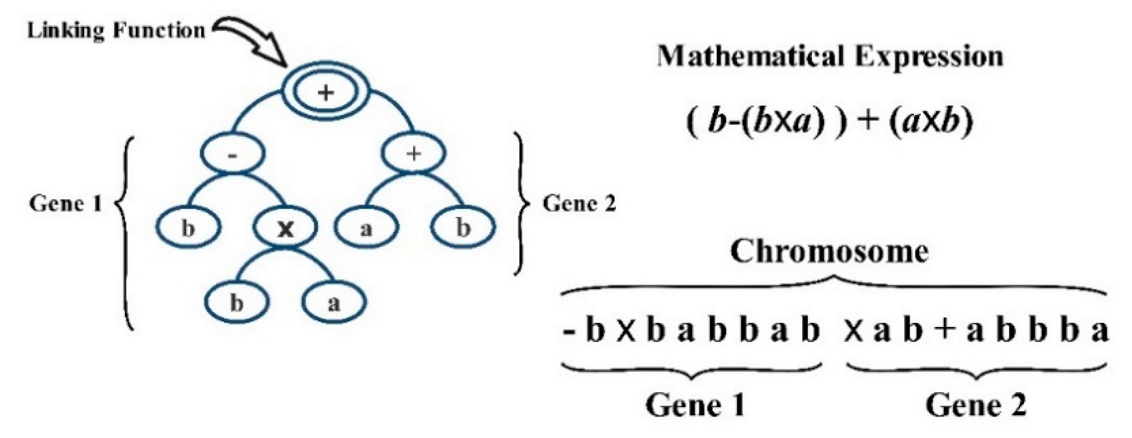
Lag Time:Figure 3a,b presents the time variation of water consumption dataset for a six-year period (from January 2011 to December 2016) and the average 24-h consumption based on City of Kelowna’s Utility report. The data were parsed into hourly maximum, minimum, and mean values for a 24-h period (Figure 3b). Figure 3b also presents a boxplot of the total mean, minimum, and maximum consumption value distributions for the six years period. Figure 3b indicates that the average consumption and minimum values have low frequency, demonstrating the highly deterministic behavior of the data. To calibrate the models, the data splinted into two folds; (1) 80% for training period (1st January 2016 to 31st December 2015); (2) 20% for test period (1st January 2016 to 31st December 2016). Water consumption estimation and forecasting of the average and minimum values are not as complex as compared to the peak consumption values. However, the maximum values exhibit a non-linear behavior which does not follow a specific pattern (i.e., appears to be random) unlike average and minimum values. Further, the maximum consumption values in a water distribution system are very important. This is because of estimation of peak consumption to supply customers’ consumption and optimize WDS pipeline to make WDS more reliable, such as managing pipeline failures, improving peak pressure, reducing leakage, etc.

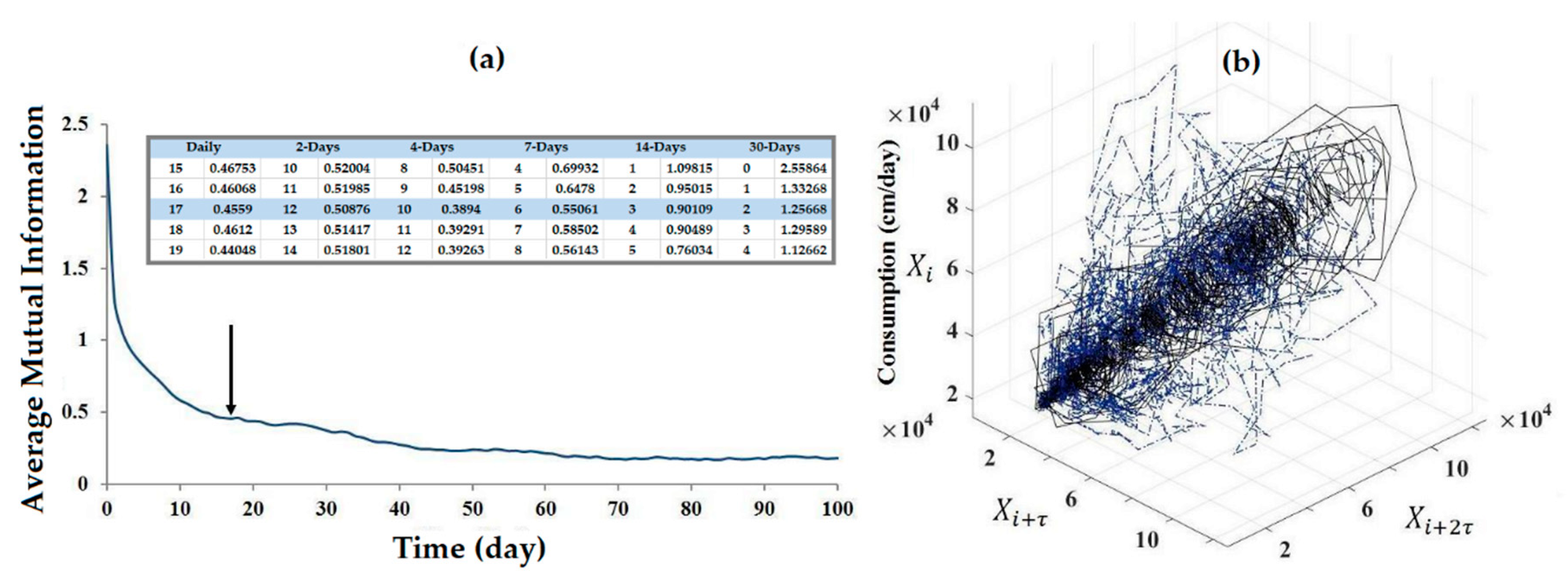
Average mutual information (AMI) was used to identify the proper lag time in this study. Figure 4a presents the first local minimum lag time of τ = 17 days for daily time series as a function of lag time. The first minimum values of AMI were at lag times of 17, 12, 10, 6, 3 and 2 for daily, 2-, 4-, 7-, 14- and 30-days (monthly) data series of the water consumption, respectively.

Table 2. Average mutual information and correlation exponent values in different temporal resolutions.

Time Scale	AMI	Ce	2LogN > Ce
Daily	17	3.50	6.67
2-Day	12	3.37	6.07
4-Day	10	3.74	5.48
7-Day	6	3.94	4.98
14-Day	3	3.83	4.38
30-Day	2	3.49	3.71

summarizes the results for all other timescales. By using the lag time of τ = 17 days, the phase-space was reconstructed, as presented in Figure 4b for daily scale. The vertical axis shows the time series and the other two axes show the same time series delayed by 17-(τ) and 34-days (2τ). This figure shows reconstructions in three dimensions; the projection attractor on the plane $\left\{x_i,x_{i+\tau },x_{i+2\tau }\right\}$ with the lag time of 17 days. When comparing the two PSR graphs in Figure 4b, the presence of attractors becomes clear for τ = 17 days (black line) comparing to τ = 1 (blue dots). Indeed, the phase space is more spread for 1-day lag time and more concentrated on attractors for 17-days lag time. Based on the figure, PSR can make a consistent set of inputs for the model that makes better results in comparison with other sets having less consistency (e.g., peak consumption represented in Figure 3b).

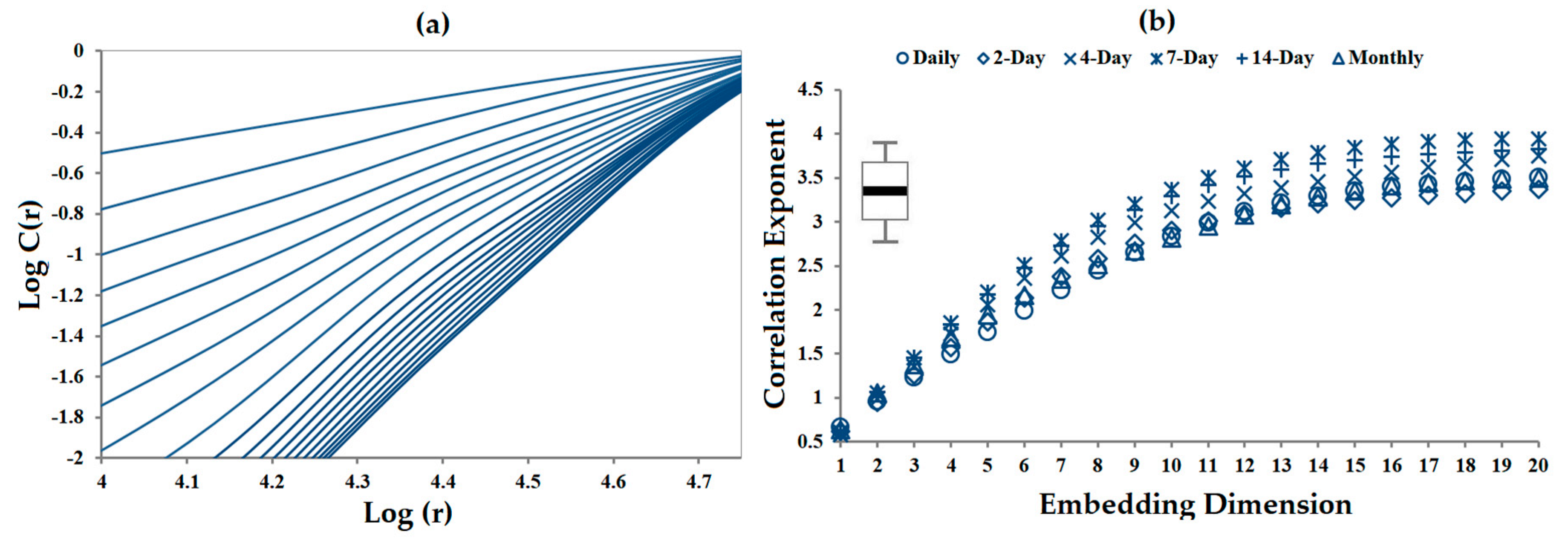
Correlation Dimension:Figure 5a plots the results for correlation integral versus log (r) for different dimensions (m) in the range of 1 to 20 for daily consumption time series. The correlation exponents, C_e (m), were determined and the results were plotted in Figure 5b to evaluate the presence of chaos in the dataset. As demonstrated in Figure 5b, the correlation exponent increases with the embedding dimension up to a certain value and then remains steady. The figure reveals that the slope of larger embedding would become constant for all temporal scales.

The embedding dimension of 17 appears to explain the dynamics of the system (1- and 2-day consumption). The correlation exponents of 3.5, 3.37, 3.74, 3.94, 3.83 and 3.49 were determined for daily, 2-, 4-, 7-, 14- and 30-day, respectively. Regarding the concept of PSR, rounding up the correlation exponent to the nearest integer informs the number of dominant variables. Thus, it can be interpreted as the number of variables that dominantly govern the temporal dynamics of water consumption, which is approximately 4 for all temporal scales. Table 2 presents the results of lag time and correlation exponent for all temporal scales. Moreover, the condition of C_e < 2 logN (with N as the number of data point) was satisfied for the chaotic temporal scales [106].

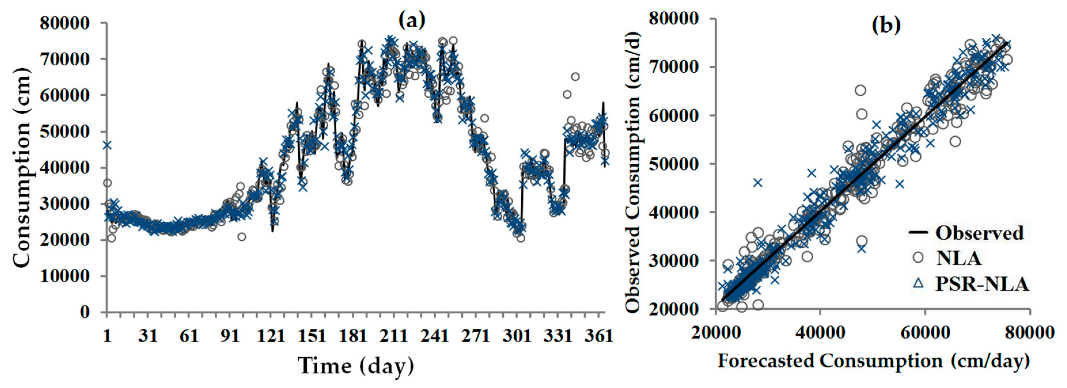
Nonlinear Local Approximation and Largest Lyapunov Exponent: The first objective in this research was to investigate the impact of PSR in the accuracy of forecasted values. Forecasted values were evaluated for the embedding dimensions (ranging from 2 to 10) at lag times 1 and 17 days to forecast 1-day-ahead and highlight the effect of embedding dimension and performance of models. For m = 2, for a lag time of 1 day, two variables D_t and D_t−1, and for m = 2, for a lag time of 17 days, two variables D_t and D_t−17, were used as input variables to forecast 1-day ahead (D_t+1). For m = 3, for the lag time of 1 and 17 days, three variables D_t, D_t−1, D_t−2 and D_t, D_t−17, D_t−34 were used as input variables to predict 1-day-ahead. Moreover, phase space was reconstructed for m > 3.

Table 3. Fitness values for NLA and PSR-NLA methods in different embedding dimension lag time and lead time.

NLA, τ = 1, T = 1				PSR-NLA, τ = 17, T = 1				τ = 1, m = 18
m	CC	RMSE *	MAE	m	CC	RMSE *	MAE	T	CC	RMSE *	MAE
1								1	0.9842	2855.6	43.07
2	0.9759	3532.1	47.85	2	0.9751	3581.7	49.09	2	0.9783	3351.6	48.02
3	0.9771	3424.8	47.34	3	0.9773	3425.3	48.01	4	0.9331	5883.5	63.03
4	0.9762	3495.5	47.74	4	0.9789	3302.9	47.30	7	0.8932	7445.8	72.49
5	0.9785	3332.0	47.08	5	0.9785	3331.7	47.10	14	0.7877	10555.0	87.76
6	0.9795	3248.6	46.13	6	0.9795	3257.8	46.79	30	0.6735	13307.6	100.44
7	0.9802	3187.3	45.49	7	0.9829	2967.1	45.80	60	0.2523	20189.1	129.71
8	0.9805	3176.4	45.65	8	0.9838	2887.9	45.22	τ = 17, m = 19
9	0.9806	3164.1	45.65	9	0.9849	2792.8	43.95	T	CC	RMSE *	MAE
10	0.9803	3193.6	45.09	10	0.9846	2828.2	44.52	1	0.9852	2772.8	43.83
11	0.9813	3098.7	44.56	11	0.9850	2792.2	43.95	2	0.9898	2295.7	39.59
12	0.9763	3495.1	48.11	12	0.9804	3189.4	46.69	4	0.9415	5504.2	61.47
13	0.9752	3578.0	48.11	13	0.9768	3457.4	48.32	7	0.9002	7211.2	71.46
14	0.9779	3378.9	47.14	14	0.9788	3303.6	47.65	14	0.8048	10147.5	86.61
15	0.9806	3169.7	46.06	15	0.9790	3290.2	47.23	30	0.6776	13265.1	95.31
16	0.9765	3491.0	47.24	16	0.9796	3250.2	46.70	60	0.4363	17784.9	118.53
17	0.9810	3139.6	45.21	17	0.9825	2995.5	45.95
18	0.9842	2855.6	43.07	18	0.9838	2894.0	45.21		* m3
19	0.9685	4088.5	44.69	19	0.9852	2772.8	43.83
20	0.9661	4209.2	45.29	20	0.9846	2833.1	44.43
Tot	0.9775	3394.2	46.30	Tot	0.9807	3142.9	46.34
Best	0.9842	2855.6	43.07	Best	0.9852	2772.8	43.83
EM	18	18	18	EM	19	19	19

presents a summary of the 1-day ahead forecasted values that reconstructed phase-space in dimensions ranging from 2 to 20 for τ = 1 and 17 days. The overall average of fitness values for all embedding dimensions CC > 0.96, RMSE < 4200 (m3/day) (8% of average daily consumption) and MAE < 49. These results can be considered as reasonable performance of the model. Table 3 reveals the optimum embedding dimension for the most accurate forecasted value in bold. Using CC, RMSE, and MAE, the optimum embedding dimension (m_opt) was found to be 18 and 19 for the lag time of 1 and 17 days, respectively. The results of nonlinear local approximation (NLA) identify the closest results of correlation exponent in optimum embedding dimension (m = 17 for correlation dimension of daily value). The similar values for the embedding dimension of daily values imply that m = 17 or 18 is the optimum dimension of the system to be used as the models’ input. The second objective was to evaluate the performance of selected m and τ. The optimum models for m = 18, τ = 1 and m = 19, τ = 17 have been applied to forecast 2-, 4-, 7-, 14-, 30- and 60-day lead time water consumption. Figure 6 compares the NLA with observed data using bolded values in Table 3.

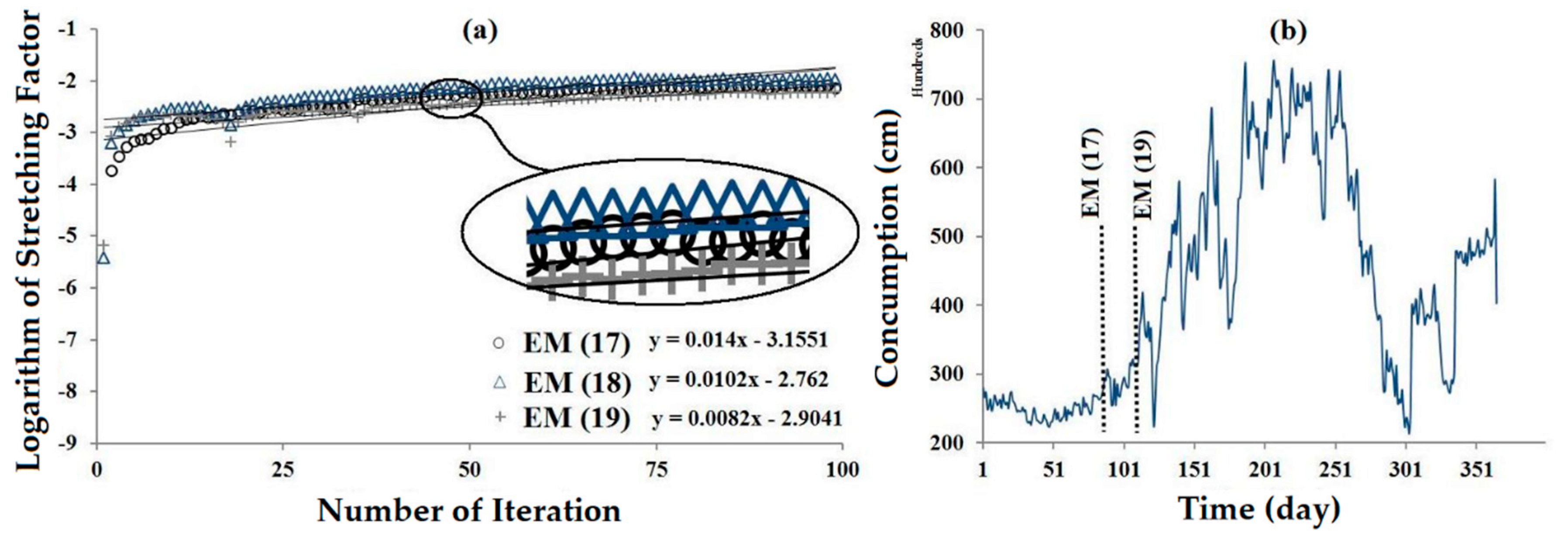
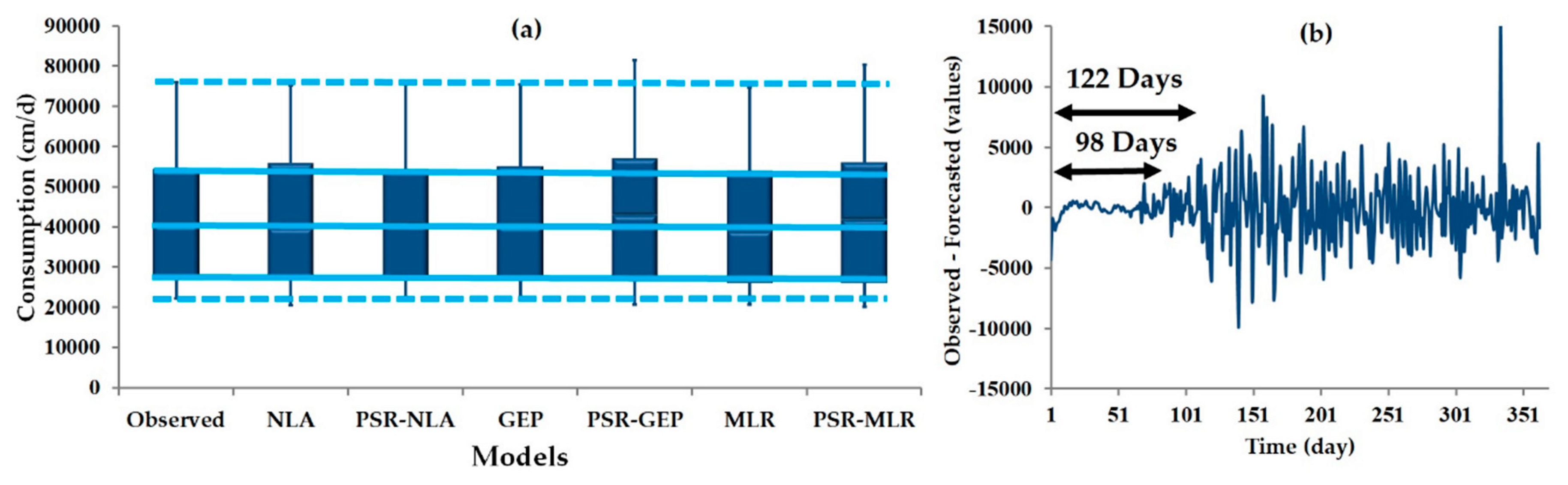
Figure 7a plots the stretching factor (S) versus the number of points (N = 100). The figure shows an overall increase in S by increasing N. Furthermore, the figure reveals two components: the first part reveals a sudden increase in S, while the second part (after N = 25) shows a more gradual increase in S. Figure 7a also indicates the best line (dashed line) fitted to the second part. Following Rosenstein et al. [101], the present study revealed ${\lambda }_{max}$ of 0.014, 0.0102 and 0.0082 for m = 17, 18 and 19, respectively. Three different values of ${\lambda }_{max}$ are considered because of the embedding dimensions range that were determined by CD, FNN, NLA and PSR-NLA, which were between 17 and 19. Note that m = 18 and 19 were determined by NLA and PSR-NLA, respectively, which gave a higher accuracy than the other embedding dimensions (see Table 3). The forecasting horizons (Δt = 1/${\lambda }_{max}$) were 72, 98 and 122 days for m = 17, 18 and 19, respectively. Moreover, m = 17 with forecasting horizon value of 72 was determined by CD. Figure 7b shows the frequency of the data is smooth from day 1 to 72. Even with the high data frequency between days 98 and 122, PSR-NLA increased the forecasting horizon from 98 days (NLA) to 122 days. Considering the results of CD, NLA, PSR-NLA, and forecasting horizon, it is reasonable to select m = 17 as the system’s optimum dimension.

Phase Space Reconstructed GEP (PSR-GEP) and Multiple Linear Regression (MLR) Models: One of the most important steps in developing an accurate model is the selection of the input variables. Input variable selection challenges the effect of the number of inputs in models’ performance. In other words, there are diminishing returns on performance based on the number of input variables selected [42]. The combinations were selected in a way that included daily consumption data with lag times of τ = 1 and 17 days. Different combinations of the time series of daily consumption were used to structure a policy for input dataset criteria. Combinations of D_t, D_t−1, D_t−2, …, D_t−20 variables were used as input data with D_t+1 (1-day time ahead) as output of the GEP and MLR model and combinations of D_t, D_t−τ, D_t−2τ, …, D_t−20τ variables were used as input data with D_t+1 as output of the PSR-GEP and PSR-MLR model (forecasting of 1 day time ahead). The combinations of arithmetic functions of $\left\{+,-,\times ,x,x^2,\sqrt{x},\log x\right\}$ and $\left\{+,-,\times ,\right\}$ were used for PSR-GEP and PSR-MLR models, respectively. Ultimately, the best combination was selected using the criteria of CC, RMSE, and MAE.

Table 4. Fitness values for GEP (gene expression programming) and PSR-GEP (phase space reconstructed GEP) methods in different embedding dimension lag time and lead time.

GEP, τ = 1, T = 1				PSR-GEP, τ = 17, T = 1				τ = 1, m = 4
m	CC	RMSE *	MAE	m	CC	RMSE *	MAE	T	CC	RMSE *	MAE
1								1	0.9764	3486.6	47.83
2	0.9757	3543.7	48.14	2	0.9789	3636.9	48.57	2	0.9494	5112.2	57.92
3	0.9761	3517.8	47.91	3	0.9788	3644.6	48.59	4	0.9130	6716.4	67.48
4	0.9764	3486.6	47.83	4	0.9789	3647.1	48.56	7	0.8652	8376.4	76.57
5	0.9760	3519.0	47.95	5	0.9789	3635.5	48.68	14	0.7810	10,734.8	88.95
6	0.9760	3520.5	48.37	6	0.9788	3649.5	48.71	30	0.6548	13,649.0	97.03
7	0.9760	3500.9	47.91	7	0.9788	3649.0	48.70	60	0.2345	20411.3	130.23
8	0.9760	3521.4	47.97	8	0.9789	3631.6	48.62	τ = 17, m = 8
9	0.9760	3511.9	47.89	9	0.9788	3653.9	48.63	T	CC	RMSE *	MAE
10	0.9760	3514.7	47.89	10	0.9788	3650.6	48.73	1	0.9789	3631.6	48.62
11	0.9760	3514.6	47.88	11	0.9788	3656.6	48.65	2	0.9553	5267.3	58.52
12	0.9760	3514.7	47.89	12	0.9787	3657.4	48.69	4	0.9227	6894.5	68.47
13	0.9760	3510.1	47.91	13	0.9789	3645.4	48.55	7	0.8713	8848.2	78.11
14	0.9760	3516.6	47.91	14	0.9787	3655.7	48.69	14	0.7782	11,571.8	91.84
15	0.9760	3510.4	47.86	15	0.9788	3650.5	48.61	30	0.6334	14,631.5	105.98
16	0.9760	3498.7	47.88	16	0.9789	3644.4	48.54	60	0.3864	18,670.2	126.20
17	0.9759	3515.1	47.89	17	0.9789	3638.9	48.56
18	0.9760	3509.7	47.85	18	0.9789	3646.6	48.57		* m3
19	0.9759	3514.8	47.93	19	0.9787	3650.6	48.74
20	0.9759	3514.2	47.90	20	0.9789	3642.5	48.51
Tot	0.9759	3519.0	47.96	Tot	0.9788	3646.5	48.62
Best	0.9764	3486.6	47.83	Best	0.9789	3631.6	48.51
EM	4	4	4	EM	8	8	20

reveals the 20 combinations of inputs and their performance with GEP and PSR-GEP models. In the table, the three criteria indicate the fourth combination of inputs (m = 4) with the lag time of 1-day, and (m = 8) with the lag time of 17 days as the best combinations of input data (reconstructed phase space) for GEP and PSR-GEP. The study reveals the following relationship for both GEP and PSR-GEP, respectively:

$$D_t=D_{t-1}+\log \left[\log (\log \left(9.58D_{t-4}\right))\times (D_{t-2}{D}_{t-3})\right]+8.253$$

(14)

$$D_t=D_{t-\tau }-0.04D_{t-4\tau }+8.03\sqrt{D_{t-4\tau }}+0.623$$

(15)

The results were not found to be more sensitive to lag time calculated by AMI (17 days) than to the 1-day lag time. However, PSR made the performance of the model better than m = 4 with 1-day lag time. Equation (14) used all four variables made by m = 4 ($D_{t-1},D_{t-2},D_{t-3},D_{t-4})$, while equation (15) only used two of the variables out of 8 variables (m = 8; $D_{t-\tau },D_{t-4\tau }$). Table 4 compares further details for GEP and PSR-GEP models for different lead times forecasted values. However, the results of both GEP and PSR-GEP are satisfactory, although they do not forecast as accurately as NLA and PSR-NLA.

Table 5. Fitness values for MLR and PSR-MLR methods in different embedding dimension lag time and lead time.

MLR, τ = 1, T = 1				PSR-MLR, τ = 17, T = 1				τ = 1, m = 17
m	CC	RMSE *	MAE	m	CC	RMSE *	MAE	T	CC	RMSE *	MAE
1								1	0.9789	3638.9	48.56
2	0.7825	11658.6	92.37	2	0.9758	3763.4	50.48	2	0.9494	5139.4	58.65
3	0.9790	3762.3	49.89	3	0.9809	3336.0	48.17	4	0.9130	6701.6	68.26
4	0.9790	3792.3	50.19	4	0.9811	3443.9	49.41	7	0.8595	8511.9	77.68
5	0.9790	3814.1	50.42	5	0.9766	3905.5	52.04	14	0.7595	11204.4	91.66
6	0.9790	3958.0	52.11	6	0.9148	22846.5	145.73	30	0.6447	13707.5	101.02
7	0.9790	4133.6	54.24	7	0.9765	3568.2	48.60	60	0.2282	20211.2	129.01
8	0.9790	4187.1	54.85	8	0.9764	3811.2	51.08	τ = 17, m = 3
9	0.9791	4432.7	57.65	9	0.9766	3568.2	48.71	T	CC	RMSE *	MAE
10	0.9792	5024.0	63.46	10	0.9766	3680.4	49.81	1	0.9809	3336.0	48.17
11	0.9792	5576.0	68.14	11	0.9767	3610.6	49.13	2	0.9555	5336.5	59.61
12	0.9792	5921.4	70.92	12	0.9767	3603.9	49.04	4	0.9232	6889.3	69.17
13	0.9793	6276.8	73.59	13	0.9766	3601.4	49.13	7	0.8723	8841.9	78.12
14	0.9793	7267.0	80.61	14	0.9767	3584.5	48.92	14	0.7790	11549.8	91.70
15	0.9794	9128.5	92.30	15	0.9769	3560.6	48.79	30	0.6344	14504.2	104.84
16	0.9794	10115.3	97.81	16	0.9769	3550.4	48.73	60	0.3859	18351.2	125.12
17	0.9789	3638.9	48.56	17	0.9769	3550.5	48.73
18	0.9794	10114.2	97.80	18	0.9769	3560.4	48.81		* m3
19	0.9794	10115.3	97.81	19	0.9768	3561.6	48.87
20	0.9795	9618.8	95.07	20	0.9769	3610.5	49.39
Tot	0.9595	6709.6	72.00	Tot	0.9738	4579.2	54.20
Best	0.9795	3638.8	48.56	Best	0.9811	3336.0	48.17
EM	20	17	17	EM	4	3	3

presents the results for the MLR model that was used as a test to compare the results of the techniques studied. The application of PSR in improving accuracy is shown in the table. Surprisingly, the best embedding dimension for MLR is 17, which was identified by CD and NLA. Additionally, as expected, PSR-MLR results are more accurate than MLR when forecasting for different lead times.

4. Discussion

A steady value of the correlation exponent in a certain embedding dimension is an indication of chaotic behavior in all six temporal scales. The correlation exponent became steady after an embedding dimension of 17 for the temporal scales. The correlation exponent results show that the 17th embedding dimension may be considered the optimum embedding dimension for this system; however, we conducted an additional investigation to better understand the optimum embedding dimension for the test case. Moreover, the saturation and constant slope of correlation exponent for all temporal scales revealed a highly chaotic behaviour exhibited by the whole system. Many studies that investigated the chaotic behaviour of the system concluded that high-resolution timescales demonstrate chaotic behaviour while the low-resolution timescale of the same time series does not exhibit chaotic behaviour.

Regarding the fractal law, it remains uncertain whether a chaotic system should have chaotic behaviour in all temporal scales; we speculate that this is an important factor to consider under this application. Based on the presented results, this study suggests that to investigate the availability of chaos in any dataset, investigation for different temporal scales is needed to indicate if the system has a chaotic behaviour, as this conclusion supports the findings presented by other researchers [54]. The present investigation of chaotic behaviour in different time scales using the test case provides enough information to evaluate the objectives of this research. However, additional study is required to make definitive conclusions regarding the findings of this study and more generally, the chaotic behaviour of consumption data. Nevertheless, the study findings provide encouraging evidence to further investigate the chaotic behaviour of water consumption values over different time scales of a dataset.

The results indicate that forecasting was more sensitive to optimum embedding dimension and lag time calculated by AMI than to the reconstructed phase space by 1-day lag time. However, the difference between the results of NLA and PSR-NLA was not considerable; the performance of PSR-NLA was better than NLA to forecast consumption values in different lead time. Moreover, m_opt = 19 provided more accurate predictions than m_opt = 18 (Table 3). Figure 8 compares observed values to the forecasted results, which highlights the negligible error in the results of PSR-NLA and GEP during the test period. Regarding the average fitness results for all dimensions, the performance of GEP is better than PSR-GEP, while the application of PSR is shown in forecasting with equal dimension and different lead times. Figure 8a shows the greatest accuracy from the results shown by PSR-NLA compared to the other models. Figure 8b shows the value of residual for forecasted consumption by PSR-NLA in two forecasting horizons. The performance of PSR-NLA in forecasting high-frequency values is shown in Figure 8b. The figure reveals that the optimum embedding dimension of 19 was more acceptable than the embedding dimension of 17 determined by the correlation function (Figure 5b).

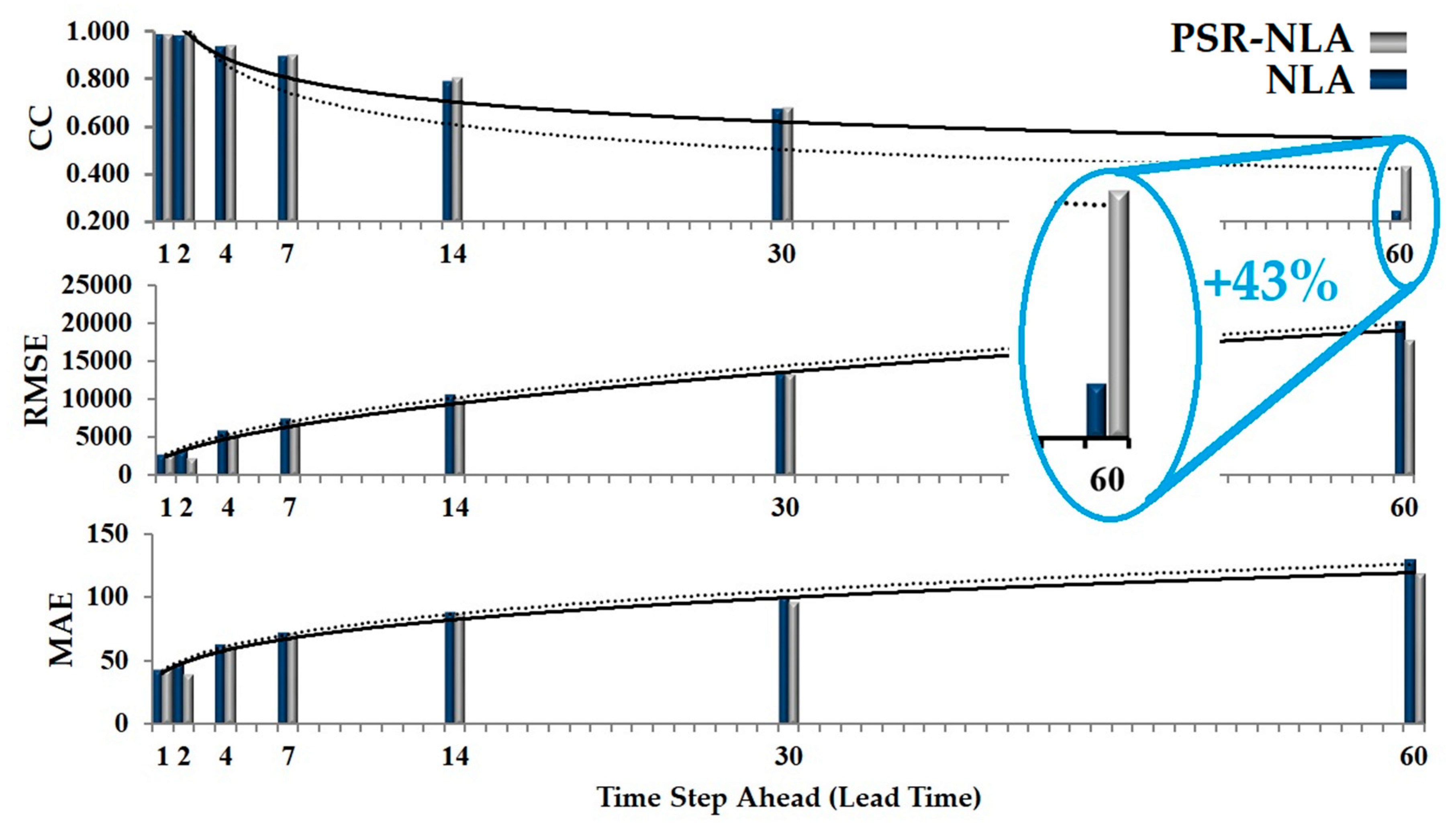
The results in Figure 8b cannot reject the optimum embedding dimension that was determined from other methods in this study. It can be concluded that the results of the 17th dimension are more reliable than those of the 19th dimension. However, the 19th dimension will offer a longer forecasting horizon. Therefore, based upon the primary goal of modeling, either dimension may be a candidate for optimum forecast modeling. The importance of embedding dimension is demonstrated when considering the small difference among the forecasted values by different embedding dimensions in all models. Therefore, it is recommended to test the optimum embedding dimension by various methods. However, the model results are quite similar; the overview of approximation for all the techniques for multiple dimensions concluded that the optimum embedding dimension is between m = 17 and m = 19, demonstrating reliability of the methods. To compare the models,

Table 6. Statistics comparison of observed and forecasted consumption in test period by the selected models.

Property	Observed	NLA τ = 1, m = 18	PSR-NLA τ = 17, m = 19	GEP τ =1, m = 4	PSR-GEP τ = 17, m = 8	MLR τ = 1, m =1 7	PSR-MLR τ = 17, m = 3
Max. value	75,620.26		✓
Min. value	21,313.72				✓
Average	42,500.82		✓
Standard deviation	16,117.34				✓
Coefficient of variation	0.38		✓
Skew	0.43		✓
Kurtosis	−1.13		✓

shows the comparison of statistics of each forecasted value with observed data. The check marks belong to the models where the results are closer to the observed values’ statistics. The results reveal the PSR technique had a positive impact on the accuracy of all models at all temporal scales, especially in high forecasting horizons. As Figure 9 shows, the performance of NLA and PSR-NLA was approximately similar for daily and 2-days ahead forecasting, but when considering the lead time with longer period, PSR-NLA was more accurate than NLA in lead time of 1- and 2-months ahead. The value of correlation coefficient for NLA and PSR-NLA shows 43% improvement. Following CC, the values of RMSE and MAE showed the performance of PSR-NLA was better than NLA in forecasting for longer lead time. Nevertheless, the slope of the fitted line for the fitness functions shows that PSR-NLA can forecast more accurate values in comparison with NLA. The results of this application of PSR may also serve useful for application in long-term forecasting, which was previously identified in the literature as a topic requiring further study in drinking water consumption modeling.

5. Conclusions

This study presented a novel approach to improve the accuracy of models in forecasting residential daily water consumption values. The residential water consumption dataset from the City of Kelowna (British Columbia, Canada) was used as a test case to forecast future consumption values using varying lead times under different temporal scales to identify models which may improve forecasting performance. A chaos approach based nonlinear local approximation was compared with previously studied forecasting methods to assess and consider the applicability of the chaotic behavior of urban consumption values to better improve forecasting performance. To investigate the existence of chaos in test data, different temporal scales were considered. The results showed all temporal scales, daily at 2-, 4-, 7-, 14- and 30-days, have chaotic behavior with similar correlation exponent values for all scales. The value of the largest Lyapunov Exponent showed the reliable time period for the models as a forecasting horizon. Dynamic investigation of explanatory variables and phase space reconstruction of the input variables based on optimum correlation dimension was considered to improve the accuracy in various periodicity and lead-times. The findings suggest that considering the chaotic behavior of consumption values by taking the forecasting horizon into account, will give insight about the behavior of data. It was recommended to investigate the performance of the models in forecasting future values with different lead-times. Considering the fitness values for the models by different lead-times within the forecasting horizon, substantial unstudied criteria remain to organize different techniques based on the behavior of the models input data. Moreover, the high results of the optimum embedding dimension in reconstructed phase space revealed that to improve the models, considering a high number of input variables is not beneficial. Therefore, this research suggested investigating the dynamic behavior of explanatory variables in modeling and forecasting problems to improve the reliability and accuracy of the water consumption models.

References

- Yousefi, P. Integrated Management Plan of Water Distribution Systems: Forecasting Approach. Ph.D. Thesis, University of British Columbia, Kelowna, BC, Canada, 2020. [Google Scholar] [CrossRef]
- Xenochristou, M.; Kapelan, Z.; Hutton, C. Using Smart Demand-Metering Data and Customer Characteristics to Investigate Influence of Weather on Water Consumption in the UK. J. Water Resour. Plan. Manag. 2020, 146, 4019073. [Google Scholar] [CrossRef]
- Water Conflict—World’s Water. Available online: https://www.worldwater.org/water-conflict/ (accessed on 14 February 2019).
- Billings, R.B.; Jones, C.V. Forecasting Urban Water Demand; American Water Works Association: Denver, CO, USA, 2008. [Google Scholar]
- Ghalehkhondabi, I.; Ardjmand, E.; Young, W.A.; Weckman, G.R. Water demand forecasting: Review of soft computing methods. Environ. Monit. Assess. 2017, 189, 313. [Google Scholar] [CrossRef]
- Sastri, T.; Valdes, J.B. Rainfall Intervention Analysis for On-Line Applications. J. Water Resour. Plan. Manag. 2008, 115, 397–415. [Google Scholar] [CrossRef]
- Odan, F.K.; Reis, L.F.R. Hybrid Water Demand Forecasting Model Associating Artificial Neural Network with Fourier Series. J. Water Resour. Plan. Manag. 2012, 138, 245–256. [Google Scholar] [CrossRef] [Green Version]
- Iwanek, M.; Kowalska, B.; Hawryluk, E.; Kondraciuk, K. Distance and time of water effluence on soil surface after failure of buried water pipe. Laboratory investigations and statistical analysis. Eksploat. I Niezawodn. Maint. Reliab. 2016, 18, 278–284. [Google Scholar] [CrossRef]
- Ghiassi, M.; Zimbra, D.K.; Saidane, H. Urban Water Demand Forecasting with a Dynamic Artificial Neural Network Model. J. Water Resour. Plan. Manag. 2008, 134, 138–146. [Google Scholar] [CrossRef]
- Jayawardena, A.W.; Gurung, A.B. Noise reduction and prediction of hydrometeorological time series: Dynamical systems approach vs. stochastic approach. J. Hydrol. 2000, 228, 242–264. [Google Scholar] [CrossRef]
- Lisi, F.; Villi, V. CHAOTIC FORECASTING OF DISCHARGE TIME SERIES: A CASE STUDY. J. Am. Water Resour. Assoc. 2001, 37, 271–279. [Google Scholar] [CrossRef]
- Cominola, A.; Giuliani, M.; Piga, D.; Castelletti, A.; Rizzoli, A.E. Benefits and challenges of using smart meters for advancing residential water demand modeling and management: A review. Environ. Model. Softw. 2015, 72, 198–214. [Google Scholar] [CrossRef] [Green Version]
- Oshima, N. Information Integration Type Chaos Theory-Based Demand Forecasting for Predictive Control of Waterworks. Water Purify Technol. 2015, 164, 6–12. [Google Scholar]
- Jain, A.; Ormsbee, L.E. Short-term water demand forecast modeling techniques—Conventional methods versus AI. J. Am. Water Work Assoc. 2002, 94, 64–72. [Google Scholar] [CrossRef]
- Kame’enui, A.E. Water Demand Forecasting in the Puget Sound Region: Short and long-Term Models. 2003, pp. 1–97. Available online: http://citeseerx.ist.psu.edu/viewdoc/download?doi=10.1.1.461.405&rep=rep1&type=pdf (accessed on 18 February 2019).
- Herrera, M.; Torgo, L.; Izquierdo, J.; Pérez-García, R. Predictive models for forecasting hourly urban water demand. J. Hydrol. 2010, 387, 141–150. [Google Scholar] [CrossRef]
- Yousefi, P.; Naser, G.; Mohammadi, H. Surface Water Quality Model: Impacts of Influential Variables. J. Water Resour. Plan. Manag. 2018, 144, 4018015. [Google Scholar] [CrossRef]
- Shabani, S.; Yousefi, P.; Adamowski, J.; Naser, G. Intelligent Soft Computing Models in Water Demand Forecasting. In Water Stress in Plants; IntechOpen: London, UK, 2016. [Google Scholar] [CrossRef] [Green Version]
- Miaou, S.-P. A stepwise time series regression procedure for water demand model identification. Water Resour. Res. 1990, 26, 1887–1897. [Google Scholar] [CrossRef]
- Jain, A.; Kumar Varshney, A.; Chandra Joshi, U. Short-Term Water Demand Forecast Modelling at IIT Kanpur Using Artificial Neural Networks. Water Resour. Manag. 2001, 15, 299–321. [Google Scholar] [CrossRef]
- Gato, S.; Jayasuriya, N.; Roberts, P. Temperature and rainfall thresholds for base use urban water demand modelling. J. Hydrol. 2007, 337, 364–376. [Google Scholar] [CrossRef]
- Bougadis, J.; Adamowski, K.; Diduch, R. Short-term municipal water demand forecasting. Hydrol. Process. 2005, 19, 137–148. [Google Scholar] [CrossRef]
- Adamowski, J.; Fung Chan, H.; Prasher, S.O.; Ozga-Zielinski, B.; Sliusarieva, A. Comparison of multiple linear and nonlinear regression, autoregressive integrated moving average, artificial neural network, and wavelet artificial neural network methods for urban water demand forecasting in Montreal, Canada. Water Resour. Res. 2012, 48. [Google Scholar] [CrossRef]
- Zhou, S.L.; McMahon, T.A.; Walton, A.; Lewis, J. Forecasting daily urban water demand: A case study of Melbourne. J. Hydrol. 2000, 236, 153–164. [Google Scholar] [CrossRef]
- Mukhopadhyay, A.; Akber, A.; Al-Awadi, E. Analysis of freshwater consumption patterns in the private residences of Kuwait. Urban. Water. 2001, 3, 53–62. [Google Scholar] [CrossRef]
- Dos Santos, C.C.; Pereira Filho, A.J. Water Demand Forecasting Model for the Metropolitan Area of São Paulo, Brazil. Water Resour. Manag. 2014, 28, 4401–4414. [Google Scholar] [CrossRef]
- Brekke, L.; Larsen, M.D.; Ausburn, M.; Takaichi, L. Suburban Water Demand Modeling Using Stepwise Regression. J. Am. Water Works Assoc. 2002, 94, 65–75. [Google Scholar] [CrossRef]
- Polebitski, A.S.; Palmer, R.N. Seasonal Residential Water Demand Forecasting for Census Tracts. J. Water Resour. Plan. Manag. 2010, 136, 27–36. [Google Scholar] [CrossRef]
- Lee, S.-J.; Wentz, E.A.; Gober, P. Space–time forecasting using soft geostatistics: A case study in forecasting municipal water demand for Phoenix, Arizona. Stoch. Environ. Res. Risk Assess. 2010, 24, 283–295. [Google Scholar] [CrossRef]
- Adamowski, J.; Karapataki, C. Comparison of Multivariate Regression and Artificial Neural Networks for Peak Urban Water-Demand Forecasting: Evaluation of Different ANN Learning Algorithms. J. Hydrol. Eng. 2010, 15, 729–743. [Google Scholar] [CrossRef] [Green Version]
- Cutore, P.; Campisano, A.; Kapelan, Z.; Modica, C.; Savic, D. Probabilistic prediction of urban water consumption using the SCEM-UA algorithm. Urban. Water J. 2008, 5, 125–132. [Google Scholar] [CrossRef]
- Adamowski, J.F. Peak Daily Water Demand Forecast Modeling Using Artificial Neural Networks. J. Water Resour. Plan. Manag. 2008, 134, 119–128. [Google Scholar] [CrossRef] [Green Version]
- Zhou, T.; Wang, F.; Yang, Z. Comparative Analysis of ANN and SVM Models Combined with Wavelet Preprocess for Groundwater Depth Prediction. Water 2017, 9, 781. [Google Scholar] [CrossRef] [Green Version]
- Firat, M.; Yurdusev, M.A.; Turan, M.E. Evaluation of Artificial Neural Network Techniques for Municipal Water Consumption Modeling. Water Resour. Manag. 2009, 23, 617–632. [Google Scholar] [CrossRef]
- Xu, Y.; Zhang, J.; Long, Z.; Chen, Y. A Novel Dual-Scale Deep Belief Network Method for Daily Urban Water Demand Forecasting. Energies 2018, 11, 1068. [Google Scholar] [CrossRef] [Green Version]
- Msiza, I.S.; Nelwamondo, F.V.; Marwala, T. Artificial neural networks and support vector machines for water demand time series forecasting. In Proceedings of the IEEE International Conference on Systems, Man and Cybernetics, Montreal, QC, Canada, 7–10 October 2007; pp. 638–643. [Google Scholar] [CrossRef] [Green Version]
- Msiza, I.S.; Nelwamondo, F.V.; Marwala, T. Water demand prediction using artificial neural networks and support vector regression. J. Comput. 2008, 3, 1–8. [Google Scholar] [CrossRef]
- Shabani, S.; Yousefi, P.; Naser, G. Support Vector Machines in Urban Water Demand Forecasting Using Phase Space Reconstruction. Procedia Eng. 2017, 186, 537–543. [Google Scholar] [CrossRef]
- Yousefi, P.; Shabani, S.; Mohammadi, H.; Naser, G. Gene Expression Programing in Long Term Water Demand Forecasts Using Wavelet Decomposition. Procedia Eng. 2017, 186, 544–550. [Google Scholar] [CrossRef]
- Shabani, S. Water Demand Forecasting: A Flexible Approach. Ph.D. Thesis, University of British Columbia, Kelowna, BC, Canada, 2018. [Google Scholar] [CrossRef]
- Ambrosio, J.K.; Brentan, B.M.; Herrera, M.; Luvizotto, E.; Ribeiro, L.; Izquierdo, J. Committee Machines for Hourly Water Demand Forecasting in Water Supply Systems. Math. Probl. Eng. 2019, 2019, 1–11. [Google Scholar] [CrossRef] [Green Version]
- Yousefi, P.; Naser, G.; Mohammadi, H. Application of Wavelet Decomposition and Phase Space Reconstruction in Urban Water Consumption Forecasting: Chaotic Approach (Case Study). In Wavelet Theory and Its Applications; IntechOpen: London, UK, 2018. [Google Scholar] [CrossRef] [Green Version]
- Yousefi, P.; Naser, G.; Mohammadi, H. Hybrid Wavelet and Local Approximation Method for Urban Water Demand Forecasting—Chaotic Approach. In Proceedings of the WDSA Conference, Kingstone, ON, Canada, 23–25 July 2018. [Google Scholar]
- Azadeh, A.; Neshat, N.; Hamidipour, H. Hybrid Fuzzy Regression–Artificial Neural Network for Improvement of Short-Term Water Consumption Estimation and Forecasting in Uncertain and Complex Environments: Case of a Large Metropolitan City. J. Water Resour. Plan. Manag. 2011, 138, 71–75. [Google Scholar] [CrossRef]
- Ahmadi, S.; Alizadeh, S.; Forouzideh, N.; Yeh, C.H.; Martin, R.; Papageorgiou, E. ICLA imperialist competitive learning algorithm for fuzzy cognitive map: Application to water demand forecasting. In Proceedings of the IEEE International Conference on Fuzzy Systems, Beijing, China, 6–11 July 2014; pp. 1041–1048. [Google Scholar] [CrossRef]
- Navarrete-López, C.; Herrera, M.; Brentan, B.; Luvizotto, E.; Izquierdo, J. Enhanced Water Demand Analysis via Symbolic Approximation within an Epidemiology-Based Forecasting Framework. Water. 2019, 11, 246. [Google Scholar] [CrossRef] [Green Version]
- Yousefi, P.; Naser, G.; Mohammadi, H. Estimating High Resolution Temporal Scale of Water Demand Time Series—Disaggregation Approach (Case Study). In Proceedings of the 13th International Conference on Hydroinformatics (HIC 2018), Palermo, Italy, 1–6 July 2018; Volume 3, pp. 2408–2416. [Google Scholar] [CrossRef]
- Kozłowski, E.; Kowalska, B.; Kowalski, D.; Mazurkiewicz, D. Water demand forecasting by trend and harmonic analysis. Arch. Civ. Mech. Eng. 2018, 18, 140–148. [Google Scholar] [CrossRef]
- Campisi-Pinto, S.; Adamowski, J.; Oron, G. Forecasting Urban Water Demand Via Wavelet-Denoising and Neural Network Models. Case Study: City of Syracuse, Italy. Water Resour. Manag. 2012, 26, 3539–3558. [Google Scholar] [CrossRef]
- Casdagli, M. Chaos and Deterministic Versus Stochastic Non-Linear Modelling. J. R Stat. Soc. Ser. B 1992, 54, 303–328. [Google Scholar] [CrossRef]
- Lorenz, E.N. Atmospheric Predictability as Revealed by Naturally Occurring Analogues. J. Atmos. Sci. 2004, 26, 636–646. [Google Scholar] [CrossRef] [Green Version]
- Sivakumar, B.; Jayawardena, A.W.; Li, W.K. Hydrologic complexity and classification: A simple data reconstruction approach. Hydrol. Process. 2007, 21, 2713–2728. [Google Scholar] [CrossRef]
- Ng, W.W.; Panu, U.S.; Lennox, W.C. Chaos based Analytical techniques for daily extreme hydrological observations. J. Hydrol. 2007, 342, 17–41. [Google Scholar] [CrossRef]
- Regonda, S.K.; Sivakumar, B.; Jain, A. Temporal scaling in river flow: Can it be chaotic? Hydrol. Sci. J. 2004, 49, 373–385. [Google Scholar] [CrossRef] [Green Version]
- Salas, J.D.; Kim, H.S.; Eykholt, R.; Burlando, P.; Green, T.R. Aggregation and Sampling in Deterministic Chaos: Implications for Chaos Identification in Hydrological Processes. June 2005. Available online: https://hal.archives-ouvertes.fr/hal-00302625/ (accessed on 29 July 2019).
- Elshorbagy, A.; Simonovic, S.P.; Panu, U.S. Estimation of missing streamflow data using principles of chaos theory. J. Hydrol. 2002, 255, 123–133. [Google Scholar] [CrossRef]
- Elshorbagy, A.; Simonovic, S.P.; Panu, U.S. Noise reduction in chaotic hydrologic time series: Facts and doubts. J. Hydrol. 2002, 256, 147–165. [Google Scholar] [CrossRef]
- Sivakumar, B.; Wallender, W.W. Predictability of river flow and suspended sediment transport in the Mississippi River basin: A non-linear deterministic approach. Earth Surf. Process. Landforms. 2005, 30, 665–677. [Google Scholar] [CrossRef]
- Zounemat-Kermani, M. Investigating Chaos and Nonlinear Forecasting in Short Term and Mid-term River Discharge. Water Resour. Manag. 2016, 30, 1851–1865. [Google Scholar] [CrossRef]
- Ghorbani, M.A.; Khatibi, R.; Danandeh Mehr, A.; Asadi, H. Chaos-based multigene genetic programming: A new hybrid strategy for river flow forecasting. J. Hydrol. 2018, 562, 455–467. [Google Scholar] [CrossRef]
- Sivakumar, B. A phase-space reconstruction approach to prediction of suspended sediment concentration in rivers. J. Hydrol. 2002, 258, 149–162. [Google Scholar] [CrossRef]
- Sivakumar, B.; Jayawardena, A.W. An investigation of the presence of low-dimensional chaotic behaviour in the sediment transport phenomenon. Hydrol. Sci. J. 2002, 47, 405–416. [Google Scholar] [CrossRef]
- Ghorbani, M.; Khatibi, R.; Asadi, H.; Yousefi, P. Inter-Comparison of an Evolutionary Programming Model of Suspended Sediment Time-Series with Other Local Models. In Genetic Programming—New Approaches and Successful Applications; IntechOpen: London, UK, 2012. [Google Scholar] [CrossRef] [Green Version]
- Petkov, B.H.; Vitale, V.; Mazzola, M.; Lanconelli, C.; Lupi, A. Chaotic behaviour of the short-term variations in ozone column observed in Arctic. Commun. Nonlinear Sci. Numer. Simul. 2015, 26, 238–249. [Google Scholar] [CrossRef]
- Ghorbani, M.A.; Kisi, O.; Aalinezhad, M. A probe into the chaotic nature of daily streamflow time series by correlation dimension and largest Lyapunov methods. Appl. Math. Model. 2010, 34, 4050–4057. [Google Scholar] [CrossRef]
- Khatibi, R.; Ghorbani, M.A.; Aalami, M.T.; Kocak, K.; Makarynskyy, O. Dynamics of hourly sea level at Hillarys Boat Harbour, Western Australia: A chaos theory perspective. Ocean Dyn. 2011, 61, 1797–1807. [Google Scholar] [CrossRef]
- Rodriguez-Iturbe, I.; Febres De Power, B.; Sharifi, M.B.; Georgakakos, K.P. Chaos in rainfall. Water Resour. Res. 1989, 25, 1667–1675. [Google Scholar] [CrossRef]
- Jayawardena, A.W.; Lai, F. Analysis and prediction of chaos in rainfall and stream flow time series. J. Hydrol. 1994, 153, 23–52. [Google Scholar] [CrossRef]
- Sivakumar, B.; Berndtsson, R.; Olsson, J.; Jinno, K.; Kawamura, A. Dynamics of monthly rainfall-runoff process at the Gota basin: A search for chaos. Hydrol. Earth Syst. Sci. 2000, 4, 407–417. [Google Scholar] [CrossRef] [Green Version]
- Maskey, M.L.; Puente, C.E.; Sivakumar, B. Temporal downscaling rainfall and streamflow records through a deterministic fractal geometric approach. J. Hydrol. 2019, 568, 447–461. [Google Scholar] [CrossRef]
- Wang, J.; Shi, Q. Short-term traffic speed forecasting hybrid model based on Chaos–Wavelet Analysis-Support Vector Machine theory. Transp. Res. Part. C Emerg. Technol. 2013, 27, 219–232. [Google Scholar] [CrossRef]
- Ravi, V.; Pradeepkumar, D.; Deb, K. Financial time series prediction using hybrids of chaos theory, multi-layer perceptron and multi-objective evolutionary algorithms. Swarm Evol. Comput. 2017, 36, 136–149. [Google Scholar] [CrossRef]
- Abdechiri, M.; Faez, K.; Amindavar, H.; Bilotta, E. The chaotic dynamics of high-dimensional systems. Nonlinear Dyn. 2017, 87, 2597–2610. [Google Scholar] [CrossRef]
- Li, M.W.; Geng, J.; Han, D.F.; Zheng, T.J. Ship motion prediction using dynamic seasonal RvSVR with phase space reconstruction and the chaos adaptive efficient FOA. Neurocomputing 2016, 174, 661–680. [Google Scholar] [CrossRef]
- Kalra, R.; Deo, M.C. Genetic programming for retrieving missing information in wave records along the west coast of India. Appl. Ocean. Res. 2007, 29, 99–111. [Google Scholar] [CrossRef]
- Ustoorikar, K.; Deo, M.C. Filling up gaps in wave data with genetic programming. Mar. Struct. 2008, 21, 177–195. [Google Scholar] [CrossRef]
- Gaur, S.; Deo, M.C. Real-time wave forecasting using genetic programming. Ocean. Eng. 2008, 35, 1166–1172. [Google Scholar] [CrossRef]
- Aytek, A.; Kişi, Ö. A genetic programming approach to suspended sediment modelling. J. Hydrol. 2008, 351, 288–298. [Google Scholar] [CrossRef]
- Ferreira, C. Gene Expression Programming in Problem Solving. In Soft Computing and Industry; Springer: London, UK, 2002; pp. 635–653. [Google Scholar] [CrossRef] [Green Version]
- Ferreira, C. Function Finding and the Creation of Numerical Constants in Gene Expression Programming. In Advances in Soft Computing; Springer: London, UK, 2003; pp. 257–265. [Google Scholar] [CrossRef] [Green Version]
- Nasseri, M.; Moeini, A.; Tabesh, M. Forecasting monthly urban water demand using Extended Kalman Filter and Genetic Programming. Expert Syst. Appl. 2011, 38, 7387–7395. [Google Scholar] [CrossRef]
- Shabani, S.; Candelieri, A.; Archetti, F.; Naser, G. Gene Expression Programming Coupled with Unsupervised Learning: A Two-Stage Learning Process in Multi-Scale, Short-Term Water Demand Forecasts. Water 2018, 10, 142. [Google Scholar] [CrossRef] [Green Version]
- Gutzler, D.S.; Nims, J.S. Interannual Variability of Water Demand and Summer Climate in Albuquerque, New Mexico. J. Appl. Meteorol. 2006, 44, 1777–1787. [Google Scholar] [CrossRef]
- Donkor, E.A.; Mazzuchi, T.A.; Soyer, R.; Alan Roberson, J. Urban Water Demand Forecasting: Review of Methods and Models. J. Water Resour. Plan. Manag. 2012, 140, 146–159. [Google Scholar] [CrossRef]
- Alvisi, S.; Franchini, M.; Marinelli, A. A short-term, pattern-based model for water-demand forecasting. J. Hydroinformatics 2006, 9, 39–50. [Google Scholar] [CrossRef] [Green Version]
- Sivakumar, B.; Berndtsson, R.; Olsson, J.; Jinno, K. Evidence of chaos in the rainfall-runoff process. Hydrol. Sci. J. 2001, 46, 131–145. [Google Scholar] [CrossRef]
- Takens, F. Detecting strange attractors in turbulence. In Dynamical Systems and Turbulence, Warwick; Springer: Berlin/Heidelberg, Germany, 1981; pp. 366–381. [Google Scholar] [CrossRef]
- Sivakumar, B. Forecasting monthly flow dynamics in the western united states: A nonlinear dynamical approach. J. Environ. Model. Softw. 2003, 17, 721–728. [Google Scholar] [CrossRef]
- Khatibi, R.; Sivakumar, B.; Ghorbani, M.A.; Kisi, O.; Koçak, K.; Farsadi Zadeh, D. Investigating chaos in river stage and discharge time series. J. Hydrol. 2012, 414–415, 108–117. [Google Scholar] [CrossRef]
- Meng, Q.; Peng, Y. A new local linear prediction model for chaotic time series. Phys. Lett. Sect. A Gen. At. Solid State Phys. 2007, 370, 465–470. [Google Scholar] [CrossRef]
- Fraser, A.M.; Swinney, H.L. Independent coordinates for strange attractors from mutual information. Phys. Rev. A 1986, 33, 1134–1140. [Google Scholar] [CrossRef] [PubMed]
- Holzfuss, J.; Mayer-Kress, G. An Approach to Error-Estimation in the Application of Dimension Algorithms. In Dimensions and Entropies in Chaotic Systems; Springer: Berlin/Heidelberg, Germany, 2011; pp. 114–122. [Google Scholar] [CrossRef] [Green Version]
- Hegger, R.; Kantz, H.; Schreiber, T. Practical implementation of nonlinear time series methods: The TISEAN package. Chaos Interdiscip. J. Nonlinear Sci. 1999, 9, 413–435. [Google Scholar] [CrossRef] [PubMed] [Green Version]
- Zounemat-Kermani, M.; Kisi, O. Time series analysis on marine wind-wave characteristics using chaos theory. Ocean. Eng. 2015, 100, 46–53. [Google Scholar] [CrossRef]
- Grassberger, P.; Procaccia, I. Measuring the strangeness of strange attractors. Phys. D Nonlinear Phenom. 1983, 9, 189–208. [Google Scholar] [CrossRef]
- Islam, M.N.; Sivakumar, B. Characterization and prediction of runoff dynamics: A nonlinear dynamical view. Adv. Water Resour. 2002, 25, 179–190. [Google Scholar] [CrossRef]
- Tongal, H.; Berndtsson, R. Impact of complexity on daily and multi-step forecasting of streamflow with chaotic, stochastic, and black-box models. Stoch. Environ. Res. Risk Assess. 2017, 31, 661–682. [Google Scholar] [CrossRef]
- Farmer, J.D.; Sidorowich, J.J. Predicting chaotic time series. Phys. Rev. Lett. 1987, 59, 845–848. [Google Scholar] [CrossRef] [PubMed] [Green Version]
- Itoh, K.-I. A method for predicting chaotic time-series with outliers. Electron. Commun. Jpn. Part III Fundam Electron. Sci. 1995, 78, 44–53. [Google Scholar] [CrossRef]
- Porporato, A.; Ridolfi, L. Nonlinear analysis of river flow time sequences. Water Resour. Res. 1997, 33, 1353–1367. [Google Scholar] [CrossRef]
- Rosenstein, M.T.; Collins, J.J.; De Luca, C.J. A practical method for calculating largest Lyapunov exponents from small data sets. Phys. D Nonlinear Phenom. 1993, 65, 117–134. [Google Scholar] [CrossRef]
- Shang, P.; Li, X.; Kamae, S. Chaotic analysis of traffic time series. Chaos Solitons Fractals 2005, 25, 121–128. [Google Scholar] [CrossRef]
- Holland, J.H. Genetic algorithms and the optimal allocation of trials. In Evolutionary Computation: The Fossil Record; Society for Industrial and Applied Mathematics: Philadelphia, PA, USA, 1998; Volume 2, pp. 443–460. [Google Scholar] [CrossRef]
- Goldberg, D.E.; Holland, J.H. Genetic Algorithms and Machine Learning. Mach. Learn. 1988, 3, 95–99. [Google Scholar] [CrossRef]
- Strategic Value Solution. Kelowna Integrated Water Suply Plan. Kelowna. 2017. Available online: https://www.kelowna.ca/city-services/water-wastewater/ (accessed on 26 February 2020).
- Ruelle, D. The Claude Bernard Lecture, 1989. Deterministic Chaos: The Science and the Fiction. Proc. R Soc. A Math. Phys. Eng. Sci. 1990, 427, 241–248. [Google Scholar] [CrossRef]
Figure 1.
Research process scheme and methodology.
Figure 2.
Expression tree and mathematical function of two gene chromosome.
Figure 3.
Time series plot of (a) daily water consumption; (b) 6-years consumption pattern within a 24-h period.
Figure 4.
(a) Average mutual information for the daily value (τ = 17); (b) reconstructed phase space by (τ and 2τ-day lag time).
Figure 5.
(a) The relation between correlation integral C(r) and r by different embedding dimensions for daily temporal scale, (b) saturation of correlation dimension Ce (m) with embedding dimension m for different temporal scales.
Figure 6.
Forecasted values for water consumption by NLA (nonlinear local approximation) and PSR-NLA (phase space reconstructed-NLA) methods in comparison with observed values (a) consumption values time series (b) scatter pilot.
Figure 7.
Estimation of largest Lyapunov exponent for daily consumption (a) for embedding dimension of 17, 18 and 19; (b) Observed values of water consumption in the test period.
Figure 8.
Performance of the models (a) box-plot of forecasted values in comparison with observed values; (b) Residual of PSR-NLA (best performance) in two forecasting horizons.
Figure 9.
Performance of NLA and PSR-NLA in time ahead forecasting by the fitness functions of Correlation Coefficient (CC); Root Mean Square Error (RMSE); Mean Absolute Error (MAE) for lead time of 1-, 2-, 4-, 7-, 14-, 30- and 60-days.