Shifting Hydrological Processes in a Canadian Agroforested Catchment due to a Warmer and Wetter Climate


1
Department of Environmental Sciences, University of Québec at Trois-Rivières, QC G8Z 4M3, Canada
2
Center for Northern Studies (CEN), Québec City, QC GV1 0A6, Canada
3
Research Centre for Watershed-Aquatic Ecosystem Interactions (RIVE), University of Québec at Trois-Rivières, Trois-Rivières, QC G8Z 4M3, Canada
4
Department of Natural Resources and Environmental Science, University of Nevada, Reno, NV 89557, USA
5
Global Water Center, University of Nevada, Reno, NV 89557, USA
*
Author to whom correspondence should be addressed.
Water 2020, 12(3), 739; https://doi.org/10.3390/w12030739
Submission received: 17 February 2020
/
Revised: 2 March 2020
/
Accepted: 4 March 2020
/
Published: 8 March 2020
(This article belongs to the Special Issue Whither Cold Regions Hydrology under Changing Climate Conditions)
Abstract
:This study examines the hydrological sensitivity of an agroforested catchment to changes in temperature and precipitation. A physically based hydrological model was created using the Cold Regions Hydrological Modelling platform to simulate the hydrological processes over 23 years in the Acadie River Catchment in southern Québec. The observed air temperature and precipitation were perturbed linearly based on existing climate change projections, with warming of up to 8 °C and an increase in total precipitation up to 20%. The results show that warming causes a decrease in blowing snow transport and sublimation losses from blowing snow, canopy-intercepted snowfall and the snowpack. Decreasing blowing snow transport leads to reduced spatial variability in peak snow water equivalent (SWE) and a more synchronized snow cover depletion across the catchment. A 20% increase in precipitation is not sufficient to counteract the decline in annual peak SWE caused by a 1 °C warming. On the other hand, peak spring streamflow increases by 7% and occurs 20 days earlier with a 1 °C warming and a 20% increase in precipitation. However, when warming exceeds 1.5 °C, the catchment becomes more rainfall dominated and the peak flow and its timing follows the rainfall rather than snowmelt regime. Results from this study can be used for sustainable farming development and planning in regions with hydroclimatic characteristics similar to the Acadie River Catchment, where climate change may have a significant impact on the dominating hydrological processes.
1. Introduction
Ongoing and future changes in air temperature and the amount and timing of precipitation can have large impacts on the hydrological cycle, such as changes to the quantity, seasonality and timing of streamflow [1,2,3,4,5]. These changes are likely to vary regionally depending on current and future regional climate conditions and catchment characteristics. In particular, climate projections at mid-latitudes in North America (40° N to 60° N) show an overall warming and increasing precipitation trend, with seasonal changes varying among regions [6]. The hydrological regime of cold regions is largely controlled by snow processes that are expected to be particularly sensitive to climate change [7,8,9,10,11,12,13,14]. Changes to snow accumulation and melt are expected to modify the timing, duration and magnitude of streamflow in the mid-latitudes of the Northern Hemisphere [15], which could redefine flooding risks as well as hydrological services, such as water supply from snowmelt runoff. The interactions between snow and vegetation play a significant role in snow accumulation [16,17], which can influence runoff volumes and timing. Snowfall intercepted by vegetation can increase sublimation losses, depending on tree species, canopy structure as well as atmospheric conditions [18,19]. Once on the ground, snow can be redistributed by wind, particularly in open and wind-exposed environments, which increases sublimation losses from blowing snow [20,21]. Snow is typically transported from sparsely vegetated and exposed terrains to densely vegetated areas and/or topographic depressions [22,23].
The traditional approach to assess climate change impact on hydrology is a “top–down” approach, where one or several hydrological models are forced by climate change scenarios from Global Circulation Models (GCMs) [24]. The spatially coarse outputs of GCMs (approximately 150–300 km) are downscaled to represent local climate conditions required by hydrological models, using either statistical or dynamical downscaling approaches [25]. Statistical downscaling relies on empirical relationships between GCMs and locally-observed climate variables, while dynamical downscaling uses GCM simulations to force initial and boundary conditions on a higher-resolution (approximately 1–50 km) regional climate model [26]. Although statistical downscaling is less computationally demanding, it requires long-term and high-quality observations to develop the empirical relationships [27], which may not be valid under future climate conditions. Dynamical downscaling, on the other hand, is physically based, but computationally more expensive as it involves higher-resolution climate models. Extensive reviews on the use of downscaling methods in hydrological climate change impact studies were made by Fowler, Blenkinsop and Tebaldi [26] and Teutschbein and Seibert [28]. Meanwhile, some have advocated the use of simpler approaches to avoid the limitations of statistical and dynamical downscaling. These approaches have been used under different names, such as arbitrary/incremental scenarios [29], sensitivity analysis [12,30], and scenario-neutral approaches [31]. The “sensitivity analysis” approach will be used in this study, where uniform and regional annual and/or seasonal climate changes are calculated and used to perturb historical time series of air temperature and precipitation. The main limitation of this method is that it does not account for changes in the variability of future climatic conditions [32]. Nevertheless, simple sensitivity analyses of hydrological models to a wide range of plausible climate conditions can reveal how some specific hydrological characteristics (e.g., flood amplitude and timing, snow cover duration and distribution) respond to climate change [24,33] and guide the need to conduct more targeted scenario-based projections. The method is particularly well suited to examine the interplay of warming temperatures and increasing precipitation that are predicted for many cold regions.
There have been a large number of snow hydrology studies performed in the Canadian Prairies [34,35,36,37,38,39,40,41] and in forest environments in Europe [42,43], Scandinavia [44,45], western Canada [18,46,47,48] and southern Québec [49,50,51,52,53,54,55]. However, some of the main cold regions hydrological processes such as blowing snow redistribution, sublimation and infiltration into frozen soils have been ignored in previous modelling studies in southern Québec. Also, to our knowledge, there has been no application of physically based hydrological models to investigate the hydrological processes and their climate sensitivity in catchments characterized by alternating agricultural fields and forest patches, which are the dominant landscapes along the south shore of the St. Lawrence River. These mosaics of forests and agricultural fields are referred to as agroforested landscapes in southern Québec [56]. The amount and timing of available water, and the length of the growing season shape the agricultural production in this region; therefore, climate change-induced modifications of hydrological conditions could have important implications for the economic development of the region. Furthermore, southern Québec suffers from water quality problems caused by erosion from agriculture soils [49,57]. As soil erosion rates are enhanced during the cold season [58], changes in winter surface runoff processes could increase soil erosion rates and further deteriorate the water quality. Therefore, there is an urgent need to better understand cold regions hydrological processes and characterize their climate sensitivity in this region. The main purpose of this study is to the explore the impacts of changes in temperature and precipitation on the hydrology of the agroforested Acadie River Catchment (45°11′ N 73°26′ W) at the catchment and landscape (agriculture vs. forest) scales. The main hydrological controls for the historical 1996–2019 period were first diagnosed using the physically based Cold Regions Hydrological Modelling (CRHM [59]) platform. Then, the model was perturbed using climate change projections and used to assess the hydrological sensitivity to climate change. This study aims to answer the following questions: (1) what are the physical processes and feedback mechanisms driving the hydrological response of the catchment to warming and increasing precipitation associated with climate change? (2) how sensitive are the hydrological processes to various climate change scenarios? and (3) how do they change across different land cover types (agriculture and forest)? The climate sensitivity analysis framework used in this study provides a useful assessment of potential hydrological changes and their driving processes under a wide range of climate change scenarios.
2. Materials and Methods
2.1. Study Area and Data
The Acadie River begins near the Canada-United States border and flows northwards over 82 km in the Montérégie region of Québec, on the south shore of the St. Lawrence River (Figure 1). It is the main tributary of the Richelieu River into which it drains at the town of Carignan. The drainage area of the Acadie River Catchment is 364 km2; however, this study excludes a small (1%) part of the catchment located in US (Figure 1) due to the lack of data.
The elevation ranges from 40 to 110 m a.s.l. (Figure 1) with gentle slopes ranging from 0° to 2°. Approximately 77% of the catchment is covered by agricultural fields with scattered forest patches (Figure 1), which is representative of the intensive farming landscape of the southern St. Lawrence lowlands [56]. In total, 17% of the catchment area is covered by forest—of which, 60% is deciduous, 27% is mixed forests and 13% is coniferous forests. The rest of the catchment (6%) is composed of urban areas, wetlands and lakes and shrubs (Figure 1).
The climate is cold and humid, with warm summers (Dfb) (Köppen climate classification [60]). Based on hourly records from the L’Acadie weather station (Figure 1) available for the 1996–2019 period (Environment and Climate Change Canada, WMO ID 71372), the mean annual and cold season (November–April) air temperature was 7.2 and −3.9 °C, respectively, while the mean annual precipitation was 1030 mm. The hydrology of the Acadie River is driven by mixed rain and snow processes, resulting in two high flow events on a normal water year. The first high flow typically occurs in early spring following snowmelt, while the second is a rainfall-runoff event in late fall. The surficial geology of the upper catchment is mainly composed of stony tills due to the geographical proximity of the Adirondack Mountains, whereas the lower catchment is mostly composed of clayey and loamy soils formed from marine and fluvial deposits [57]. Organic soils formed from the gradual accumulation of organic matter are present across the catchment, and discontinuous glacial till is found below the marine and fluvial sediments [57]. Given the flat topography and poor drainage of soils (particularly clay), tile drainage is used extensively to remove excess water from the surface and rootzone. These subsurface tiles drain into a system of ditches, or surface canals, that are connected to the river network (Figure 1). The soil textures in the catchment are 40% clayey, 25% till deposits, 17% organic soil, 10% sandy, 4% loamy and 4% gravelly, which were acquired from Québec Research and Development Institute for the Agri-Environment (IRDA) at a 1:50,000 scale. The land use datasets were obtained from Québec Ministry of Forests, Wildlife and Parks (MFFP) and La Financière Agricole du Québec (FADQ) for both non-agricultural lands and cropping systems. While the main crop is soybeans (40%) followed by corn (34%) [57], different crop types such as vegetables (mainly potatoes and onions), wheat, barley and other cereal grains are also cultivated in the agricultural lands. A 1 × 1 m resolution LIDAR-based digital elevation model (DEM) was obtained from MFFP. The stream and open channel drainage networks were acquired from Québec Ministry of Energy and Natural Resources (MERN). Hourly air temperature, wind speed and relative humidity data within the catchment were acquired for the 1996–2019 period from the L’Acadie weather station (Figure 1) maintained by Environment and Climate Change Canada (ECCC). Gaps in the data were filled with data from four other ECCC weather stations (Ste-Clotilde, McTavish, St-Anne de Bellevue and Frelighsburg) located within a radius of 50 km from the geometric center of the study area. The 1.6% gaps were filled by a principal component analysis (PCA) with the expectation-maximization algorithm [61]. This method uses a cross-validation procedure prior to filling the missing data to detect the number of statistically significant empirical orthogonal functions (EOFs) used for reconstructing the missing data. The temperature was spatially distributed at the catchment based on an environmental lapse rate of 0.005 °C m−1 [62]. Hourly solar radiation was extracted for the L’Acadie weather station from the database of Hydro-Québec (available at https://www.simeb.ca:8443/index_fr.jsp). Daily total precipitation data were extracted from the 0.1° × 0.1° gridded climate data produced by the Québec Ministry of Sustainable Development, Environment, and Fight against Climate Change (MELCC). This dataset was created by spatially interpolating (kriging) quality-controlled observations of permanent weather stations from the Programme de Surveillance du Climat du Québec (PSC) and ECCC [62]. The main advantage of this dataset is its long coverage from 1961 to present. Bajamgnigni Gbambie et al. [63] compared the different gridded precipitation datasets and their implication for hydrological modelling in Québec and found that the MELCC data showed the best performance in catchments located on the south shore of the St. Lawrence River. Daily river discharge measured at the L’Acadie discharge gauge (Figure 1) were extracted from the database of Québec Center of Water Expertise (CEHQ) (www.cehq.qc.ca) for the 1996–2019 period. Observations of snow depth and density were obtained from the Hemmingford snow course station, located within a mixed forest patch a few kilometers away from the catchment (Figure 1). Snow surveys have been performed by the MELCC every two weeks during winter and spring since the 1980s, using 10 fixed points uniformly distributed along a 300 m transect representative of the surrounding landscape [64]. Snow depth is measured by probing with a snow tube at eight locations surrounding the fixed points and the results are averaged. Density is measured by weighting the snow tube sample taken at the center of the fixed point and the result is multiplied by the mean snow depth to estimate SWE at the point. Finally, the mean SWE at the site is obtained by averaging the SWE measured at the 10 points along the transect. Errors on site-averaged SWE are not reported, but federal snow tubes are known to overestimate SWE, typically by 0% to 11% [65]. Additional snow depth and density measurements were made for the winters of 2018 and 2019 along survey transects at agricultural and forest sites, where soil temperature/moisture probes were installed (Figure 1). SWE values were then averaged to represent landscape-scale SWE.
2.2. Hydrological Model Configuration
The Cold Regions Hydrological Model (CRHM) platform [59] was used to develop a hydrological model for the Acadie River Catchment. The CRHM platform has been successfully used in several catchments in Canada [7,48,66], as well as other cold environments such as the Spanish Pyrenees [67], Patagonia [68], northwest US [12], western China [69] and Svalbard Archipelago [70]. The CRHM platform has a modular structure that allows creating purpose-oriented models with great emphasis on physically based parameterizations. Modules within the CRHM platform represent hydrological processes of varying complexity that can be selected depending on available data [71]. Cold regions hydrological processes included in the CRHM platform include snow accumulation and redistribution by wind, sublimation of canopy-intercepted snowfall, energy budget snowmelt, and infiltration into frozen soils. Hydrological response units (HRUs) with different biophysical attributes (e.g., vegetation cover and soil type) [72] were used as the main spatial units for mass and energy balance calculations. Table 1 provides the hydrological processes and modules used to simulate the hydrology of the Acadie River Catchment.
HRUs were delineated using a combination of six soil types (clayey, till deposits, organic soil, sandy, loamy and gravelly) and seven land use classes (agriculture, urban, deciduous forest, mixed forest, coniferous forest, shrub and wetland), resulting in 37 HRUs. The open drainage canals and river network were also defined as two separate HRUs, resulting in a total of 39 HRUs. Elevation, slope and aspect were not used for HRU delineation as they vary little over the catchment. Mean physiographic parameters for each HRU (i.e., area, altitude, slope, aspect and latitude) were extracted from the 1 m DEM and HRU maps processed in ArcGIS. Soil parameters such as soil texture, thickness of the recharge and lower soil layer, porosity and saturated hydraulic conductivity were derived from studies in neighboring catchments [55,93,94,95,96], a soil survey report from the Agriculture and Agri-Food Canada [97], and a groundwater study in the Montérégie region [98]. The pore size distribution indices were defined based upon soil textures [99]. Summer leaf area index (LAI) for the agricultural and forest HRUs were transferred from the neighboring Chateauguay River basin [55]. An LAI value of 3 m2 m−2 was assigned to agricultural HRUs (mainly corn and soybean), while summer LAI values for forest HRUs varied between 2.2 and 6 m2 m−2 depending on forest type (deciduous, mixed and coniferous). Coniferous and mixed forests were assigned a winter LAI of 2.2 and 0.5 m2 m−2, respectively [55]. An LAI of 0.4 m2 m−2 was assigned to deciduous forests, which is similar to the value used for aspen forests in the Canadian Prairie during winter [100]. Maximum canopy snow load capacity values for the forest HRUs were assigned based on previous studies performed in western Canada [38,100,101], using values of 5.9, 2.1, 0.5 kg m−2 for coniferous, mixed and deciduous forests, respectively. Based on the local measurements (Figure 1) from November to April in 2018 and 2019, initial average fall volumetric soil moisture content was assigned as 30%, and soil temperature was estimated at +2 °C (at 15 cm soil depth) prior to snowmelt, which controls the heat flux from the soil to the snowpack base [80]. While this positive soil temperature was chosen to best represent the observed near surface (0–30 cm) temperature before snowmelt, shallow soil freezing was also observed in the agricultural fields in the winter of 2019. With this in mind, the frozen soil infiltration algorithm [85] was included in the model (Table 1).
Blowing snow transport is simulated from the agriculture towards the forest HRUs, following the sequence from agriculture to wetland, shrub, drainage canal and finally to forest HRUs [34]. The maximum value for the liquid water holding capacity of snow was set to 0.01 mm mm-1 as suggested by Marks, Kimball, Tingey and Link [80]. Saturation excess water in soils is added to the subsurface flow in the agricultural fields to emulate the effect of subsurface tile drainage. Regarding runoff routing, agricultural fields were first routed to the drainage canals, and then the outflow from the drainage canals routed to the river network, while other HRUs were routed directly to the streamflow network. Similar to the method used by Cordeiro et al. [102], the routing length was determined as the median distances from the centroid of each HRU to the closest drainage canal for agricultural HRUs, and as the median distances from each HRU to the streamflow network for non-agricultural HRUs.
Given that the Hemmingford snow survey station (Figure 1) is located a few kilometers outside of the catchment, a point-scale snowmelt model was constructed for the Hemmingford station using the CRHM platform. The point-scale model was forced with disaggregated hourly precipitation from daily precipitation extracted from the MELCC gridded climate data at the Hemmingford station (Figure 1), and the infilled hourly meteorological air temperature, relative humidity, wind speed and solar radiation at the L’Acadie weather station. This point-scale model was used to validate the snowpack and canopy parameters, which were assigned based on the literature, as presented in the previous section. As such, the model did not require a calibration. The SWE observations at the Hemmingford snow station were compared with the point-scale model simulations for the 1996–2019 period.
The evaluation of the hydrological model performance was carried out using statistical performance measures, including the Nash–Sutcliffe efficiency (NSE [103]; Equation (1)), the Kling–Gupta efficiency (KGE [104]; Equation (2)), the percent bias (PBIAS; Equation (3)), the root mean square error (RMSE; Equation (4)) and the root mean square error-observations standard deviation ratio (RSR [105]; Equation (5)).
where is the number of samples, is the linear correlation between observations and simulations, and , are the mean and standard deviation of the observed values (), respectively. , are the mean and standard deviation of the simulated values (), respectively. The NSE is an often-used metric in hydrology, which determines the relative magnitude of the residual variance compared to the measured data variance [103]. While NSE = 1 indicates perfect fit between the observations and simulations, NSE = 0 indicates that the model simulations have the same explanatory power as the mean of the observations. KGE is based on a decomposition of NSE into its constitutive components (correlation, bias and variability) in the context of hydrological modelling [104]. While KGE = 1 indicates perfect correspondence between simulations and observations, it has been argued that KGE < 0 indicates that the mean of observations provides better estimates than simulations [106]. Therefore, any positive value of NSE and KGE suggests that the model has some predictive power and higher values indicate better model performance. A positive value of PBIAS indicates a model overestimation, while a negative value indicates an underestimation. The RMSE is a weighted measure of the difference between observation and simulation. The RSR standardizes RMSE using the standard deviation of the observations. The lower RSR, the lower the RMSE, and the better the model simulation performance [105].
2.3. Climate Sensitivity Analysis
Climate sensitivity analysis was performed at both the catchment and landscape (agriculture vs. forest) scale. The range of projected changes in temperature and precipitation was based on ensemble climate model projections available for the administrative regions of Québec [107]. These projections were produced from a set of 11 downscaled global climate simulations produced from the CMIP5 ensemble for two periods (2041 to 2070 and 2071 to 2100) and two greenhouse gas emission scenarios (moderate: RCP 4.5 and high: RCP 8.5) for the province of Québec [107]. The reference period for the projections was 1981–2010. The 1-d quantile mapping [108] method was employed to downscale the raw global climate simulation outputs to a finer resolution [109]. Guided by the scenarios produced for the Montérégie administrative region where the Acadie River Catchment is located, temperature warming up to 8 °C (0–8 °C at 1 °C intervals) and an increase in total precipitation up to 20% (0–20%, 5% intervals) were considered in the sensitivity analysis. Thus, these scenarios encompass the most extreme end-of-the-century projection within the spread (10–90 percentile) of ensemble projections under the high emission RCP 8.5 scenario [107]. The different combinations of warming and precipitation changes were applied to the historical data and the hydrological run for each perturbed climate record, for a total of 45 individual climate scenarios. The baseline scenario of no change in air temperature and precipitation (Δt = 0 °C and P = 100%: reference run) represents the historically averaged observed data over the 1996–2019 period. The scenario of “Δt = 8 °C and P = 120%” stands for a warming of 8 °C and an increase of 20% in averaged precipitation relative to the reference run.
3. Results
3.1. Historical Simulations
3.1.1. Point-Scale Snow Simulations
Observed and simulated SWE at the Hemmingford snow survey station was compared for the 1996–2019 period (Figure 2). The Nash–Sutcliffe efficiency (NSE) is 0.57 over the 23-year simulation. The root mean square error (RMSE), correlation coefficient and mean percent bias (PBIAS) are 28 mm, 0.84 and −10% for the simulation period, respectively. SWE is mostly underestimated during low snowpack years, which is likely due to uncertainties in the gridded precipitation dataset, parameters selections and limitations of the snow model (SNOBAL) [80], which was originally developed to simulate deep snowpacks. Despite some discrepancies, these results are considered to be adequate for the purpose of this study.
3.1.2. Simulation of Snow Mass Fluxes
Simulated SWE was compared against snow surveys at the agriculture and forest sites for the winters of 2018 and 2019 (Figure 3). The observed spatial heterogeneity in snow accumulation within the agricultural sites and forest patches is represented by the error bars (Figure 3). The simulations show that the annual peak SWE is higher in the deciduous forest than in agricultural fields for both winters (Figure 3). For the forest site, the mean percent biases are 10% and −6%, and the RMSEs are 35 mm and 25 mm for the winters of 2018 and 2019, respectively. For the agriculture site, the mean percent biases are −19% and 50%, and the RMSEs are 21 mm and 41 mm for the winters of 2018 and 2019, respectively. While the overall absolute accuracy is similar between the two sites, relative errors are greater in fields where the snowpack is thinner. Hence, the model performs relatively better in forests than in fields, which could be partly explained by the fact that thinner snowpacks are more difficult to simulate by SNOBAL [80]. The model could not capture the melt event leading to the complete disappearance of snow cover in agriculture fields in mid-March 2019 (Figure 3c), which is the main reason for the high percent bias and root mean square error. It is important to note that although there was no snow cover observed in agriculture fields in mid-March 2019, there was an ice layer with a thickness of 5 to 10 cm over the fields. Disregarding the mid-March 2019 event, the mean percent bias and RMSE becomes 23% and 11 mm, respectively, for the winter of 2019. For both agriculture and forest sites, the statistical performance measures show a better performance in the winter of 2019, which had wetter conditions and a thicker snowpack.
Figure 4 shows simulated SWE at the catchment and landscape (i.e., agriculture, deciduous forest, mixed forest and coniferous forest) scale for the 1996–2019 period. The mean annual peak SWE at the catchment scale is 65 mm and occurs on February 25, with large inter-annual variability ranging between 21 mm and 118 mm (Figure 4a). Landscape scale simulated SWE shows that peak SWE is on average higher in the deciduous and mixed forest, followed by agricultural fields and coniferous forest (Figure 4b). The accumulated SWE in the coniferous forest is lower than in the mixed and deciduous forests because of the greater sublimation losses from canopy-intercepted snowfall, as the maximum canopy interception load capacity and LAI are significantly higher in the coniferous forests than in the deciduous and mixed forests. The bare agricultural fields suffer from sublimation losses and transport of blowing snow, resulting in lower snow accumulation than in deciduous and mixed forests. These processes were further investigated by examining snow mass balance at the landscape scale.
Daily average cumulative snow mass fluxes and mean daily SWE for the 1996–2019 period for agriculture and forest (i.e., deciduous, coniferous and mixed forest HRUs) landscape units are presented in Figure 5. Snowmelt is the largest outflux at approximately 200 mm year−1 for both landscape units, representing approximately 15% of the mean annual precipitation and 85% of the mean annual snowfall. Snowpack sublimation reaches an average of 23 mm year−1, which is approximately 10% of the mean annual snowfall, with a negligible difference between landscape units. Overall, total sublimation losses from both snowpack and blowing snow reach 33.7 mm year−1 (14.3% of annual snowfall) in fields, while in forests snowpack and canopy sublimation together account for 46.4 mm year−1 (19.4% of annual snowfall).
Sublimation from canopy interception exhibits large spatial variability among the forest types (Figure 5b). Canopy interception loss reaches approximately 40% of the mean annual snowfall in the coniferous forest, whereas it is 12% and 3% of the mean annual snowfall in the mixed and deciduous forest, respectively. Higher canopy interception losses in the coniferous canopies is attributed to the greater canopy snow interception loads and LAIs. However, the dominant deciduous (60%) and mixed (27%) forest cover in the catchment shape the average canopy interception loss in the forest, which is on average 24 mm year−1 (10% of the mean annual snowfall) (Figure 5). Simulated blowing snow transport out of agricultural fields is only 5 mm year−1 and the blowing snow sublimation is approximately 10 mm year−1, which together represent approximately 6% of the mean annual snowfall. On the other hand, blowing snow transport into forests reaches 19 mm year−1 which is higher than blowing snow transport out of agricultural fields. This difference is due to the larger area of agricultural fields and also because snow is transported from other HRUs such as open drainage canals once their storage capacity is reached. Although total sublimation losses are greater in forests than in agricultural fields, the annual peak SWE is slightly higher in forests (65 mm) than in agriculture fields (59 mm), as also observed from snow surveys (Figure 4). This can be explained with the redistribution of the blowing snow from the agriculture and other HRUs to the forest.
3.1.3. Simulation of Streamflow and Water Fluxes
Simulated daily streamflow was compared against measurements at the outlet of the catchment for the 1996–2019 period (Figure 6). The Nash–Sutcliffe efficiency (NSE), Kling–Gupta efficiency (KGE), percent bias (PBIAS) and the ratio of root mean square error to the standard deviation of measured discharge (RSR) for the 23 year simulation period are 0.51, 0.71, 2.4% and 0.70, respectively. Simulated streamflow properly represents flow duration curves (Figure 6b); however, low flows (high exceedance probability, >0.9) are overestimated. The cumulative mean daily discharge (Figure 6c) shows good performance with a mean bias of 2.4% at the end of the water year. However, the model slightly overestimates winter streamflow (Figure 6c), which corresponds to overestimated high exceedance flows (Figure 6b). The peak flow timing and magnitude are generally well represented by the model (Figure 6a,b). The inter-annual variability of observed annual streamflow volume is approximately 30%, which is slightly higher than that of simulated streamflow (23%) (Figure 6c). Uncertainties in simulated streamflow may arise from uncertainties in the forcing data, parameters uncertainty and errors in the model structure. Despite these reasonable discrepancies, both the timing and volume of streamflow are overall well simulated, suggesting a good model performance.
On average, 77% of the mean annual precipitation is rainfall and 23% is snowfall (Figure 7). The snowfall and rainfall ratios exhibit large inter-annual variability with the snowfall ratio varying between 17% and 34%, and the rainfall ratio between 66% and 83% (Figure 7). On average, 6% of the total rainfall occurs during winter months (Dec-Jan-Feb), while almost half of the total rainfall is observed from May to September. The evapotranspiration (ET) loss constitutes the largest water loss term (462 mm year−1) (Figure 7), representing 45% of total annual precipitation. ET exhibits a relatively low inter-annual variability with an annual standard deviation of 28 mm (Figure 7). The simulated ET is very similar to the annual evapotranspiration value (487 ± 42 mm) calculated for a neighboring basin (Chateauguay River Basin) for the 1963–2001 period [55]. The ratio of annual evapotranspiration to annual precipitation is also comparable to that simulated for the 1971–2001 period for the neighboring Pike River agricultural watershed using the SWAT model (47%) [49]. Annual total sublimation loss including snowpack sublimation, canopy interception sublimation and blowing snow sublimation is 36 mm (Figure 7), which is approximately 3% of the annual precipitation and 15% of the mean annual snowfall. Mean annual sublimation shows an inter-annual variability of ±15 mm (Figure 7). The sublimation losses are simulated between mid-November and mid-April when the snow cover is present. During the same period, ET is suppressed due to the presence of snow cover. Once the snow cover disappears, ET begins and almost 60% of the total ET occurs between mid-April and August. Mean annual streamflow is 453 mm (Figure 7), resulting in an average runoff ratio of 0.44. The mean annual runoff exhibits large inter-annual variability (±110 mm), which mostly results from the high interannual variability of rainfall (±115 mm) (Figure 7). Annual average groundwater recharge rate is 79 mm (8% of total annual precipitation) over the 23 year period, with an inter-annual variability of ±26 mm (Figure 7). The historically averaged groundwater recharge rate is comparable to the simulated annual groundwater recharge of 86 ± 10 mm in the neighboring Chateauguay River Basin using the physically based HELP (Hydrologic Evaluation of Landfill Performance) numerical model for the 1963–2001 period [55]. The ratio of groundwater recharge to annual precipitation is also comparable to that (8%) simulated for the Pike River Watershed [49]. The largest increase in both cumulative streamflow and groundwater recharge is observed between April and May (Figure 7), which can be explained by the snowmelt contribution to both fluxes. High evapotranspiration levels in summer months decrease soil moisture levels, thereby limiting the amount of excess soil moisture available for percolation, which in turn results in very low groundwater recharge rates in summer months (Figure 7).
3.2. Climate Sensitivity
3.2.1. Climate Sensitivity of Snow Regime and Mass Balance Components
Historically, snowfall represents 23% of the mean annual precipitation for the reference period (ΔT = 0; P = 100%) (Figure 7), which decreases down to 11% and 8% for a 5 and 8 °C warming scenario, respectively, regardless of changes in the mean annual precipitation (Table 2). With a warming of 2 °C and no change in precipitation, peak SWE decreases by 70% and occurs 8 days earlier (Table 2). The same scenario delays the snow onset date (SOD) by 25 days and advances the snow disappearance date (SDD) by 14 days, shortening the snow cover duration (SCD) by 39 days (Table 2). In case of a 5 °C warming and no change in precipitation, the peak SWE drastically shifts from late February to late December and decreases below 10 mm. Under the same scenario, SDD advances by more than a month and SCD decreases to 132 days per year (Table 2). With the maximum warming of 8 °C, peak SWE decreases by more than 90%. A 20% increase in precipitation would only buffer 28% of the warming induced peak SWE decline for a +2 °C scenario, and 7% and 3% for the +5 and +8 °C scenarios, respectively. Hence increasing precipitation could only counterbalance less than a third of the SWE decline under a moderate (+2 °C) warming scenario.
Along with the simulated decline in SCD and snowmelt, the mean snowmelt rate also exhibits a decline under all warming scenarios. However, it is important to note that the snowmelt rate under a 2 °C warming scenario with 20% increase in precipitation slightly increases compared to the reference period. In addition, all warming scenarios lead to more frequent mid-winter snowmelt events, resulting in several snow accumulation maxima during the snow season (Figure 8).
The climate response surfaces demonstrate that the timing and magnitude of annual peak SWE is very sensitive to warming (Figure 9). Peak SWE decreases under all scenarios where warming occurs (Figure 9a), while peak SWE increases by 10% to 60% in response to increasing precipitation alone (Figure 9b). There is a positive sensitivity zone on the response surface where peak SWE increases (blue surface on Figure 9b) in response to increasing precipitation and limited warming (<1 °C). However, once further warming occurs, peak SWE decreases regardless of simulated changes in precipitation. Considering that the catchment already has a relatively warm and wet cold season, small changes in temperature generate large changes in snowfall ratios (Table 2) that result in a stronger sensitivity of peak SWE as shown by the closer contours between 0 and 2 °C warming (Figure 9a,b). Warming causes a considerable shift in the timing of peak SWE towards earlier dates (Figure 9c). A more pronounced sensitivity of peak SWE timing is observed for warming between 2 and 3 °C, as shown by the closer contours in Figure 9c. This strong sensitivity can be explained by the occurrence of several seasonal snow accumulation maxima due to more frequent mid-winter snowmelt events in warmer winters (Figure 8). Although multiple snow accumulation peaks are also simulated for warming up to 2 °C, the annual SWE peak remains towards the end of winter. However, when warming reaches 3 °C, the peak SWE simulated in early January becomes the annual peak, which explains the shift in annual peak SWE date by more than a month (Figure 9c).
As shown by Figure 9d, changes in snow cover duration (SCD) are mostly driven by warming and not by increasing precipitation. This is because the declining snowfall ratios, caused by warmer temperatures, shorten both the onset and termination of the snow season. Figure 9e shows that the snowmelt rate is primarily influenced by warming and to a lesser extent by increasing precipitation. If warming is not accompanied by an increase in precipitation, then snowmelt rates decrease. This occurs because with reduced snow accumulation in response to warming, snow melts earlier and at lower rates under lower available solar energy. On the other hand, the snowmelt rate could increase when low to moderate warming is accompanied by increasing precipitation. For instance, a 1 °C warming and a 20% increase in precipitation result in a 10% increase in the snowmelt rate (Figure 9e). This can be explained by the fact that the thicker snowpack persists longer into the spring, which combined with warming temperatures, increase the amount of energy available to melt the snow.
The responses of peak SWE to warming air temperatures and increasing precipitation in agriculture and forest landscapes (Figure 10a,b) are similar to that of the catchment average (Figure 9a). Here, peak SWE in forest landscape is obtained by aggregating peak SWEs in deciduous, mixed and coniferous forest HRUs. There is a considerable decline in peak SWE in response to warming temperature in both landscapes (Figure 10a,b). The peak SWE decreases below 10 mm in both landscapes when warming exceeds 4 °C and precipitation remains unchanged. The sensitivity of peak SWE in forests is more pronounced than in agriculture fields for warming between 0 and 2 °C, as shown by the closer contour lines in Figure 10c. The peak SWE in agriculture fields becomes slightly higher than in the forests when the warming reaches 2 °C (Figure 10c). This can be explained by changes in blowing snow transport in response to warming, such that less snow is transported into the forest under warmer temperatures, which is due to the increasing bond strength and cohesion of snow as it warms [110].
Table 3 summarizes the changes in key snow processes with respect to selected climate change scenarios for the agriculture fields and forests. The values in Table 3b are the aggregated changes over the forest types (deciduous, mixed and coniferous). Snow erosion (drift out) from agricultural fields and snow transport to forested areas (drift in) decline by 50% in response to a 2 °C warming without changing precipitation (Table 3). A warming of 5 °C leads to a decline in snow transport by more than 80% even if precipitation increases by 20% (Table 3). Accordingly, blowing snow sublimation in agriculture fields declines considerably with warming (>85% with 5 °C warming), while snowpack sublimation is relatively less sensitivity to warming (<50% with 5 °C warming, Table 3a). Apart from an insignificant increase (0.3%) in the sublimation ratio in agriculture fields for a 2 °C warming, this ratio declines for the rest of the warming scenarios.
Snowpack sublimation and canopy sublimation in forests are less sensitive to a 2 °C warming (decline by <21%, Table 3b) than the blowing snow influx (decline by 53%, Table 3b). The declines in canopy sublimation are most likely due to more rapid and earlier unloading of snow with warmer temperatures. The sublimation ratio in forests increases up to 5 °C warming (with no increase in precipitation) and then declines for 8 °C warming. The sublimation ratio in forests is higher than that in agriculture fields during the reference period, and this difference accentuates under warming scenarios. Snowmelt shows a considerable decline in response to warming for both agriculture and forests (approximately 50% for 5 °C warming, Table 3), due to decreasing snowfall ratios. Within the 0–2 °C warming zone, the peak SWE in forests decreases faster than in agriculture fields (Figure 10c and Table 3). Eventually, a warming of 2 °C leads to a homogenization of peak SWE among the agriculture and forest landscapes (Figure 10c), due to reduced redistribution and sublimation of blowing snow from agriculture fields to forests, and decreased canopy sublimation in the forest.
3.2.2. Climate Sensitivity of Streamflow Regime and Water Balance Components
The Acadie River Catchment has a mixed snowmelt/rainfall hydrological regime and in a warmer future, it is expected to shift toward a more rainfall-dominated regime (Figure 11a). The ratio of snowmelt volume to mean annual streamflow volume changes from 43% in the reference period to 32%, 23% and 16% for the 2, 5 and 8 °C warming scenarios, respectively. With a 2 °C warming and no change in precipitation, the annual peak daily flow decreases by 21% and occurs 3 months earlier (mid-January) than for the reference period (mid-April) (Figure 11a). The annual peak daily flow declines by 37% and occurs in mid-December under 8 °C warming and no change in precipitation (Figure 11a). In case of 2 °C warming accompanied by a 20% increase in precipitation, the annual peak daily discharge shows an insignificant increase (0.02%) (Figure 11a,b), but a 3 month shift in timing from mid-April to mid-January, increasing winter flows (Figure 11a). This effect can also be seen from the increase in flows with exceedance probability between 0.2 and 0.8 under 2 °C warming with a 20% increase in precipitation (Figure 11b). In the reference period, the Acadie River mean hydrograph exhibits two peaks flow following snowmelt in spring: the first peak occurs early April, followed by a second, slightly greater peak some ten days later (Figure 11a). With a 20% increase in precipitation and no warming, the second peak becomes more distinct while the first peak becomes higher than the second one (Figure 11a). The increase in high flows (exceedance probability lower than 0.1) under a 20% increase in precipitation and no warming can also be seen in Figure 11b. The low flows (exceedance probability higher than 0.8), on the other hand, exhibit an increase with a 20% increase in precipitation regardless of warming (Figure 11b).
The response surfaces of the magnitude and timing of annual peak discharge, and total annual discharge, are presented along with projected changes in annual temperature and precipitation for the periods 2041–2070 and 2071–2100 under a moderate emission scenario (RCP 4.5) and a high emission scenario (RCP 8.5) [111] (Figure 12). Increasing precipitation could cause an increase in annual peak daily discharge by up to 60%, depending on the warming and increase in precipitation. This zone of positive sensitivity of peak discharge is delineated by the 0% contour in Figure 12a, below which the peak discharge exhibits an increase. In this positive sensitivity zone, the increase in precipitation is enough to counterbalance the negative impact of warming on the peak discharge. Increasing peak daily discharge might thus represent the short-term response of peak discharge to climate change, before more significant warming (Figure 12d) depletes the snowpack and causes peak discharge to decline and shift from the spring to winter. This sensitivity zone is particularly interesting considering the recent flood events in southern Québec [112,113], versus the long-term projection of reducing SWE and peak discharge. For instance, a warming of 1.2 °C increases the annual peak daily discharge by 2% if there is an increase in precipitation by 12%, whereas the same amount of warming causes peak daily discharge to decline by 15% if there is only a 1% increase in precipitation. Both of these scenarios are within the uncertainty range of projected changes in annual temperature and precipitation for the 2041–2070 period under a moderate emission scenario RCP 4.5 (Figure 12d). Meanwhile, when the warming exceeds 2 °C, as projected under both moderate and high emission scenarios (Figure 12d) for the mid and end of century, the peak daily discharge declines regardless of changes in precipitation (Figure 12b). Warming scenarios lead to considerable shifts in the timing of annual peak discharge towards earlier dates (Figure 12b). With a 1.2 °C warming and a 12% increase in precipitation (Figure 12d), the peak discharge shifts by 20 days earlier, while a precipitation increase of less than 3% under the same warming level shifts the peak discharge 50 to 80 days earlier, i.e., before peak SWE.
These results show that a higher peak daily discharge could occur earlier in response to limited warming (<1.5 °C) if precipitation increase sufficiently, which highlights the considerable uncertainty in future peak daily discharge caused by uncertainties in projected precipitation. Meanwhile, when warming exceeds 1.5 °C, the peak daily discharge occurs before peak SWE regardless of the precipitation increase. For instance, a 2 °C warming and 20% increase in precipitation advances the timing of peak SWE by only eight days from February 25 to February 17 (Figure 9c), the same warming scenario without precipitation change causes the annual peak daily discharge timing to shift from April 11 to January 13 (Figure 12b). This highlights that a warming beyond 1.5 °C causes a transition in the flow regime of the Acadie River Catchment from a mixed snowmelt/rainfall to rainfall dominated regime, with the seasonality of precipitation dictating the magnitude and timing of the annual peak discharge (Figure 12a). Total annual discharge, on the other hand, appears much more sensitive to increasing precipitation than to warming (Figure 12c), which contrasts with the response of peak SWE (Figure 9a,b). Total annual discharge decreases by 2% with a 1 °C warming, however, an increase of 7% is simulated if this 1 °C warming occurs with an increase in precipitation of only 5%. The decrease in annual discharge volume caused by a 5 °C increase in temperature could be completely counterbalanced with an increase in precipitation of 5%.
The rainfall ratio is simulated to increase between 6% and 12%, depending on the amount of warming (Table 4). Increasing evapotranspiration rates occur under all warming and increasing precipitation scenarios (Table 4). In terms of seasonal changes in streamflow, the mean winter streamflow increases under warmer temperatures, which can be explained by the increasing rainfall ratios and more frequent snowmelt events in warmer winters. The mean winter streamflow increases by 45% and 71% under a 2 °C warming and 2 °C + 20% precipitation increase, respectively. A 20% increase in precipitation with no warming results in an unchanged rainfall ratio but an increase in total rainfall in winter, which together cause the smallest increase (9%) in winter mean runoff. The same scenario increases the mean spring streamflow by 39%, which is due to the greater amount of snow accumulation and associated snowmelt contribution as well as higher amount of rainfall. If only warming air temperatures are considered, mean streamflow declines during both spring and summer (Table 4). On the other hand, mean summer streamflow increases in response to increasing precipitation even under warmer temperatures which drive higher evapotranspiration rates, which means that increasing rainfall can counteract the enhanced evaporation losses in terms of streamflow volume generation.
In Table 4, the snowmelt infiltration ratio (%) is calculated as the ratio of snowmelt infiltration volume to total snowmelt volume, whereas the rain infiltration ratio (%) represents the ratio of rainfall infiltration volume to effective rainfall volume (total rainfall minus evaporation from canopy interception). Infiltration rates during the cold season are governed by rainfall infiltration (33% in winter and 53% in spring) rather than snowmelt infiltration (4.2% in winter and 4% in spring) (Table 4), due to the fact that frozen soil algorithm [85] limits the snowmelt infiltration. Warming causes a general decrease in the snowmelt infiltration ratio but an increase in the rainfall infiltration ratio. Under warming with no increase in precipitation, the winter snowmelt infiltration ratio declines by 1.4 to 3.7% (Table 4), which could be explained by the higher initial soil moisture saturation before snowmelt events caused by higher rainfall ratios and also more frequent mid-winter melt events. For instance, with a 2 °C warming, the rainfall ratio in winter increases from 28% to 56% and the total number of snowmelt days in January and February increases by 11 days, which in turn lead to greater soil moisture saturation. The rainfall infiltration ratio in winter increases by 9 to 12% in response to warming (Table 4), which can be explained with the fact that there is an increase in rainfall fraction and rainfall infiltration is not limited by the snow cover [85]. In spring, the snowmelt infiltration ratio declines by 1% (Table 4) with a 2 °C warming, which can be explained with declining snow accumulation and melt available for infiltration. Under warming-only scenarios, rainfall infiltration in spring increases by 2% due to higher rainfall ratios. An increase in precipitation by 20% with no warming causes an increase in the spring snowmelt infiltration ratio by 2.4% and a decrease in winter snowmelt infiltration by less than 1%, whereas rainfall infiltration ratios in both seasons exhibit a decline. Warmer temperatures cause smaller snowmelt infiltration ratios even if there is a 20% increase in precipitation, whereas rainfall infiltration ratios become higher. In summer, for the reference period, more than 90% of the effective precipitation infiltrates, which changes between −5% and 1%, depending on the climate change scenario (Table 4). Overall, changes in summer are lower than those in spring and winter. Therefore, changes in winter and spring conditions explain most of the decreases in surface runoff ratio in response to warming (Table 4). It is important to note that mimicking subsurface tile drainage plays a role in this response, since replacing snowmelt by rainfall with warming could have produced saturation excess runoff, however, this saturation excess water is added to the subsurface flow rather than surface flow. There is also an increase in both winter and annual groundwater recharge rates under all warming scenarios (Table 4).
A model falsification was performed to assess the impact of frozen soil infiltration process on the partitioning between surface and subsurface runoff, and on annual peak streamflow (Table 5). Annual streamflow declines from 468 mm to 414 mm for the reference period when the frozen soil infiltration process in removed from the model (Table 5). The results show that removing the frozen soil infiltration process reduces the surface runoff ratio by 40%, from 43% to 3.2% for the reference period (Table 4 and Table 5). This is due to snowmelt infiltrating rather than forming infiltration excess surface runoff when the frozen soil infiltration parameterization is disabled [85]. The small amount of surface runoff generated is thus uniquely from infiltration excess rainfall and/or snowmelt when frozen soils are not considered, since all saturation excess water is assumed to drain through the subsurface tiles. Surface runoff becomes less sensitive to warming with the falsification of frozen soil infiltration (Table 5) compared to when frozen soil infiltration is considered (Table 4). This is because the infiltration rates in winter and spring, which are driving the changes in surface runoff ratios (Table 4), are not primarily driven by peak snow accumulation anymore as opposed to when the frozen soil infiltration algorithm is used [85]. Therefore, the declines in peak SWE caused by warming scenarios (Table 2) do not result in significant changes in surface runoff ratios (Table 5). The model falsification also indicates that annual peak streamflow would reduce by 17% for the reference period when frozen soils do not limit infiltration (Table 4 and Table 5).
4. Discussion
Snow accumulation in the Acadie River Catchment has historically shown a large inter-annual variability (Figure 4a) due to its high sensitivity to climatic conditions. Moreover, drastic changes in snow accumulation regime are simulated under warming scenarios regardless of precipitation. This is in line with the known high temperature sensitivity of snow in the relatively mild cold regions of the warmer sectors of the Dfb (cold climate with warm summers) climate zone [60]. The decline in peak SWE caused by 1 °C warming cannot be compensated even with a 20% increase in precipitation (Figure 9b). Although there is a decrease in the sublimation ratio under this scenario, the decrease in snowfall ratio predominates and causes reduced snow accumulation. The peak SWE shows the highest sensitivity in the 0–2 °C warming zone, declining by 25%–35% per °C, which is higher than the 7% per °C reduction for the Svalbard Archipelago [70], the 7% per °C reduction for Yukon [7], the 15% per °C reduction for the Swiss Alps [114], the 11%–20% per °C reduction for the Spanish Pyrenes [67,115] and the 20% per °C reduction for the Washington Cascades [116]. The greater sensitivity of SWE in the Acadie River Catchment is likely due to the warmer temperatures in this region than in the other study areas. Snow accumulation exhibits several peaks due to more frequent mid-winter snowmelt events within the 0–2 °C warming range (Figure 8), and the first peak occurring in early January becomes dominant when warming reaches 3 °C. Therefore, the peak SWE date shows its highest sensitivity in the 2–3 °C warming band (Figure 9c) and marks the transition from a snowmelt dominated to a rainfall dominated streamflow regime. Increasing precipitation leads to higher peak SWE only if the warming is less than 1 °C (Figure 9a), which may represent the transient, short-term response of the catchment to climate change for the next decades.
Under present climate conditions, annual drift out (snow erosion) from agricultural fields were low (2% of annual snowfall) compared to the prairies and steppe environments where snow erosion rates range from 30% to 75% of annual snowfall [20,117]. This is mostly due to higher bond strength and cohesion of snow resulting from relatively higher winter air temperatures in the Acadie River Catchment, which in turn leads to higher wind speed thresholds required to initiate snow saltation [110]. Simulated average peak SWE was slightly higher in forests than in agriculture fields under recent climate, in agreement with field observations (Figure 5). However, the snow accumulation in these two landscape units become uniform when warming reaches 2 °C (Figure 10). This uniformization is explained by the decrease in blowing snow transport and sublimation due to increased snow cohesion under warming [110] and decreasing canopy sublimation.
Snowmelt is an important contributor to groundwater recharge (Figure 7), in agreement with other studies [118,119,120]. While the decline in snowmelt (Table 2) caused by warmer temperatures was expected to result in lower groundwater recharge rates, annual groundwater recharge increased instead. This is driven by significant increases in groundwater recharges during winter due to increasing mid-winter snowmelt events, as shown by previous studies [121,122,123,124]. The results show that shallower snowpacks caused by warmer temperatures melt earlier and more slowly under most of the warming scenarios considered, which is in line with the “slower snowmelt in a warmer world” hypothesis [125]. Some other studies also reported that earlier snowmelt occurring at a time of year with lower solar elevations resulted in slower snowmelt rates in different cold regions such as Spain [67], the western US [126,127,128] and south western Canada [128]. In contrast, the results also show that increasing precipitation under limited warming (≤2 °C) can compensate the slower melt rates caused by warming and even accelerate snowmelt rates depending on the amount of increase in precipitation. Furthermore, some studies have also reported increasing snowmelt rates in the future such as in an Arctic headwater basin (Canada), where a 6 °C warming and a 40% increase in precipitation was projected under the RCP 8.5 scenario [129]. This suggest that there are competing mechanisms that depend on the degree of warming and projected changes in precipitation that can either increase or decrease snowmelt rates, and that those mechanisms may vary regionally depending on historical conditions.
The peak streamflow was found to consistently shift towards earlier dates under warmer temperatures, which have also been projected for other catchments in southern Québec [49,51,52]. The magnitude of the annual peak daily streamflow shows a non-linear response to warming and increasing precipitation. While the peak spring flow decreases under most scenarios when warming exceeds 1.5 °C, the peak flow was found to increase within a restricted climate envelope (Figure 12a). Hence, higher and earlier peak flows might represent the short term, transient response of peak flow to warming and increasing precipitation, increasing flooding risks on the short term. On the other hand, although greater warming causes a decline in spring peak flow, winter flows are projected to increase, in line with the higher winter streamflow projections for different catchments in Québec [49,51,52,130] and in some other cold regions [11,44,131]. Greater winter flows can cause extreme flooding and ice jamming, resulting in significant damages [130]. In addition, changes in the streamflow timing and volume can have significant repercussions on reservoir operations for flood control and hydropower generation. Both the direction of change in peak spring flow under limited warming (<1.5 °C), and the amount of increasing winter flow under greater warming (>1.5 °C), will strongly depend on the projected changes in precipitation (Figure 12), highlighting the significant uncertainty in changes to peak discharge and flood risks, as precipitation is typically the most uncertain variable of climate projections. The falsification of frozen soil infiltration processes resulted in drastic declines in surface runoff ratios (Table 4 and Table 5), suggesting that this process is very important on the partitioning between surface and subsurface flows and overall streamflow generation in catchments with extensive subsurface tile drainage such as the Acadie River Catchment.
5. Conclusions
A physically based hydrological model was created using the CRHM platform to simulate the hydrological cycle over 23 years in an agroforested catchment in southern Québec, Canada. The model showed a reasonable performance against discontinuous SWE observations and daily streamflow measurements. A possible range of impacts of climate change on catchment hydrology was obtained by perturbing the model with warming hourly air temperatures from 1 to 8 °C and increasing daily total precipitation from 0% to 20%. The positive sensitivity zone encountered in peak streamflow response surfaces suggests a possibility for increased flood risks in the very near future (1–2 decades) given the uncertainties in precipitation projections, while longer-term warming was found to severely deplete the snowpack and reduce peak streamflow. The results of this study also have important implications for farming communities in the Acadie River Catchment. This study indicates a decreasing snow cover duration under warming temperatures, which in turn could extend the farming season. The overall agricultural production could also benefit from the increase in annual available water (annual streamflow) in response to increasing precipitation. On the other hand, higher soil moisture due to increasing rainfall ratios in warmer springs could limit the agricultural production. Considering that the catchment presents water quality issues related to soil erosion [57], and that in cold agricultural catchments, soil erosion rates during the snowmelt period can exceed those occurring during other seasons of the year [58,132], the changes in snowmelt and streamflow dynamics could alter soil erosion dynamics. Soil erosion could increase due to earlier snowmelt, increased rainfall ratios, and more frequent snowmelt events caused by higher winter and spring temperatures.
The hydrological model built in this study could be used to assess the impacts of climate change on snow accumulation and associated runoff under different tilling practices by changing the vegetation heights over the agricultural fields in the Acadie River Catchment. Future research will aim to investigate the impact of runoff changes on soil erosion rates in response to climate change scenarios. In addition, considering that Acadie River Catchment is representative of the typical agroforested landscapes with relatively warm winters across the south shore lowlands of the St. Lawrence River Watershed, the results found in this study could be extrapolated to nearby catchments with similar landscape and climate. Furthermore, since this model includes all the major physical processes at play in this type of environments, it would be relatively easy to apply it in similar environments or similar landscapes located in the warmer sectors of the Dfb climate class, which have been shown to be particularly sensitive to warming [15]. The model is particularly well suited to analyze the interactions between the hydrological processes at play, and to assess their sensitivity to changes in temperature and precipitation. It is important to note that the climate sensitivity framework used in this study only considers mean changes in air temperature and precipitation; therefore, changes in inter-annual variability or potential changes to other atmospheric variables such as humidity and wind speed were not considered. Future changes in precipitation frequency could have important hydrological impacts [133,134,135,136]. Nevertheless, the climate sensitivity analysis allowed understanding how key hydrological processes could shift under a wide range of climate change scenarios, in a fast and easy way, providing useful guidance for further top–down, model-based climate impact assessments. It is worth noting that there are different sources of uncertainty in this study. For instance, the lack of long-term snow observations in agricultural fields prevents a more robust validation of the snow model. There is thus a need for additional, long-term monitoring of snow conditions in agricultural fields in the Acadie River Catchment and elsewhere in southern Québec. In addition, some of the model parameters were transferred from studies in catchments with similar hydrological conditions, which introduces uncertainties to the modelling. Future studies should perform detailed sensitivity analyses to quantify the uncertainty in simulations due to parameter uncertainty.
Author Contributions
Conceptualization, C.K. and S.C.; methodology, O.A., C.K. and S.A.K.; formal analysis, O.A. and C.K.; data curation, O.A.; writing—original draft preparation, O.A.; writing—review and editing, C.K., S.C. and S.A.K.; supervision, C.K. and S.C.; project administration, C.K.; funding acquisition, C.K. and S.C. All authors have read and agreed to the published version of the manuscript.
Funding
This research was funded by the Natural Sciences and Engineering Council of Canada, grant number RGPIN-2015-03844 (C. Kinnard) and RGPIN-2017-06571 (S. Campeau) and the Canada Research Chair program, grant number 231380 (C. Kinnard).
Acknowledgments
A special thanks goes to the members of GlacioLab for their help during our fieldworks. We also would like to thank John Pomeroy and Logan Fang, who provided support and resources required to learn the Cold Regions Hydrological Modelling platform.
Conflicts of Interest
The authors declare no conflict of interest. The funders had no role in the design of the study; in the collection, analyses, or interpretation of data; in the writing of the manuscript, or in the decision to publish the results.
References
- Donnelly, C.; Greuell, W.; Andersson, J.; Gerten, D.; Pisacane, G.; Roudier, P.; Ludwig, F. Impacts of climate change on European hydrology at 1.5, 2 and 3 degrees mean global warming above preindustrial level. Clim. Chang. 2017, 143, 13–26. [Google Scholar] [CrossRef] [Green Version]
- DeBeer, C.M.; Wheater, H.S.; Carey, S.K.; Chun, K.P. Recent climatic, cryospheric, and hydrological changes over the interior of western Canada: A review and synthesis. Hydrol. Earth Syst. Sci. 2016, 20, 1573. [Google Scholar] [CrossRef] [Green Version]
- Kundzewicz, Z.W.; Pińskwar, I.; Brakenridge, G.R. Changes in river flood hazard in Europe: A review. Hydrol. Res. 2017, 49, 294–302. [Google Scholar] [CrossRef]
- Burn, D.H.; Whitfield, P.H. Changes in cold region flood regimes inferred from long-record reference gauging stations. Water Resour. Res. 2017, 53, 2643–2658. [Google Scholar] [CrossRef]
- Wilson, D.; Hisdal, H.; Lawrence, D. Has streamflow changed in the Nordic countries?—Recent trends and comparisons to hydrological projections. J. Hydrol. 2010, 394, 334–346. [Google Scholar] [CrossRef]
- Allen, M.R.; Barros, V.R.; Broome, J.; Cramer, W.; Christ, R.; Church, J.A.; Clarke, L.; Dahe, Q.; Dasgupta, P.; Dubash, N.K. IPCC Fifth Assessment Synthesis Report-Climate Change 2014 Synthesis Report; Intergovernmental Panel on Climate Change: Geneva, Switzerland, 2014. [Google Scholar]
- Rasouli, K.; Pomeroy, J.W.; Janowicz, J.R.; Carey, S.K.; Williams, T.J. Hydrological sensitivity of a northern mountain basin to climate change. Hydrol. Process. 2014, 28, 4191–4208. [Google Scholar] [CrossRef]
- Stewart, I.T.; Cayan, D.R.; Dettinger, M.D. Changes toward earlier streamflow timing across western North America. J. Clim. 2005, 18, 1136–1155. [Google Scholar] [CrossRef]
- Huntington, J.L.; Niswonger, R.G. Role of surface-water and groundwater interactions on projected summertime streamflow in snow dominated regions: An integrated modeling approach. Water Resour. Res. 2012, 48, W11524. [Google Scholar] [CrossRef] [Green Version]
- Molini, A.; Katul, G.G.; Porporato, A. Maximum discharge from snowmelt in a changing climate. Geophys. Res. Lett. 2011, 38, L05402. [Google Scholar] [CrossRef] [Green Version]
- Huziy, O.; Sushama, L.; Khaliq, M.; Laprise, R.; Lehner, B.; Roy, R. Analysis of streamflow characteristics over Northeastern Canada in a changing climate. Clim. Dyn. 2013, 40, 1879–1901. [Google Scholar] [CrossRef] [Green Version]
- Rasouli, K.; Pomeroy, J.W.; Marks, D.G. Snowpack sensitivity to perturbed climate in a cool mid-latitude mountain catchment. Hydrol. Process. 2015, 29, 3925–3940. [Google Scholar] [CrossRef]
- Harder, P.; Pomeroy, J.W.; Westbrook, C.J. Hydrological resilience of a Canadian Rockies headwaters basin subject to changing climate, extreme weather, and forest management. Hydrol. Process. 2015, 29, 3905–3924. [Google Scholar] [CrossRef]
- Mahmood, T.H.; Pomeroy, J.W.; Wheater, H.S.; Baulch, H.M. Hydrological responses to climatic variability in a cold agricultural region. Hydrol. Process. 2017, 31, 854–870. [Google Scholar] [CrossRef]
- Aygün, O.; Kinnard, C.; Campeau, S. Impacts of climate change on the hydrology of northern midlatitude cold regions. Prog. Phys. Geogr. Earth Environ. 2019. [Google Scholar] [CrossRef]
- Pomeroy, J.; Gray, D. Snowcover accumulation, relocation and management. Bull. Int. Soc. Soil Sci. 1995, 88, 422–423. [Google Scholar]
- Varhola, A.; Coops, N.C.; Weiler, M.; Moore, R.D. Forest canopy effects on snow accumulation and ablation: An integrative review of empirical results. J. Hydrol. 2010, 392, 219–233. [Google Scholar] [CrossRef]
- Ellis, C.; Pomeroy, J.; Brown, T.; MacDonald, J. Simulation of snow accumulation and melt in needleleaf forest environments. Hydrol. Earth Syst. Sci. 2010, 14, 925–940. [Google Scholar] [CrossRef] [Green Version]
- Hedstrom, N.; Pomeroy, J. Measurements and modelling of snow interception in the boreal forest. Hydrol. Process. 1998, 12, 1611–1625. [Google Scholar] [CrossRef]
- Pomeroy, J.; Gray, D.; Landine, P. The prairie blowing snow model: Characteristics, validation, operation. J. Hydrol. 1993, 144, 165–192. [Google Scholar] [CrossRef]
- Pomeroy, J.; Li, L. Prairie and arctic areal snow cover mass balance using a blowing snow model. J. Geophys. Res. Atmos. 2000, 105, 26619–26634. [Google Scholar] [CrossRef] [Green Version]
- Essery, R.; Pomeroy, J. Vegetation and topographic control of wind-blown snow distributions in distributed and aggregated simulations for an Arctic tundra basin. J. Hydrometeorol. 2004, 5, 735–744. [Google Scholar] [CrossRef]
- Liston, G.E.; Haehnel, R.B.; Sturm, M.; Hiemstra, C.A.; Berezovskaya, S.; Tabler, R.D. Simulating complex snow distributions in windy environments using SnowTran-3D. J. Glaciol. 2007, 53, 241–256. [Google Scholar] [CrossRef] [Green Version]
- Peel, M.C.; Blöschl, G. Hydrological modelling in a changing world. Prog. Phys. Geogr. 2011, 35, 249–261. [Google Scholar] [CrossRef]
- Salathé, E.P., Jr.; Mote, P.W.; Wiley, M.W. Review of scenario selection and downscaling methods for the assessment of climate change impacts on hydrology in the United States Pacific Northwest. Int. J. Climatol. J. R. Meteorol. Soc. 2007, 27, 1611–1621. [Google Scholar] [CrossRef]
- Fowler, H.J.; Blenkinsop, S.; Tebaldi, C. Linking climate change modelling to impacts studies: Recent advances in downscaling techniques for hydrological modelling. Int. J. Climatol. J. R. Meteorol. Soc. 2007, 27, 1547–1578. [Google Scholar] [CrossRef]
- Tang, J.; Niu, X.; Wang, S.; Gao, H.; Wang, X.; Wu, J. Statistical downscaling and dynamical downscaling of regional climate in China: Present climate evaluations and future climate projections. J. Geophys. Res. Atmos. 2016, 121, 2110–2129. [Google Scholar] [CrossRef] [Green Version]
- Teutschbein, C.; Seibert, J. Regional climate models for hydrological impact studies at the catchment scale: A review of recent modeling strategies. Geogr. Compass 2010, 4, 834–860. [Google Scholar] [CrossRef] [Green Version]
- Smith, J.B.; Mendelsohn, R.O. The Impact of Climate Change on Regional Systems: A Comprehensive Analysis of California; Edward Elgar Publishing: Cheltenham, UK; Northampton, MA, USA, 2007. [Google Scholar]
- Keller, F.; Goyette, S.; Beniston, M. Sensitivity analysis of snow cover to climate change scenarios and their impact on plant habitats in alpine terrain. Clim. Chang. 2005, 72, 299–319. [Google Scholar] [CrossRef]
- Prudhomme, C.; Wilby, R.L.; Crooks, S.; Kay, A.L.; Reynard, N.S. Scenario-neutral approach to climate change impact studies: Application to flood risk. J. Hydrol. 2010, 390, 198–209. [Google Scholar] [CrossRef] [Green Version]
- MacDonald, R.J.; Byrne, J.M.; Boon, S.; Kienzle, S.W. Modelling the potential impacts of climate change on snowpack in the North Saskatchewan River Watershed, Alberta. Water Resour. Manag. 2012, 26, 3053–3076. [Google Scholar] [CrossRef]
- Blöschl, G.; Viglione, A.; Montanari, A. Emerging approaches to hydrological risk management in a changing world. In Climate Vulnerability: Understanding and Addressing Threats to Essential Resources; Elsevier Inc., Academic Press: Amsterdam, The Netherlands, 2013. [Google Scholar] [CrossRef]
- Fang, X.; Pomeroy, J. Modelling blowing snow redistribution to prairie wetlands. Hydrol. Process. Int. J. 2009, 23, 2557–2569. [Google Scholar] [CrossRef]
- Fang, X.; Pomeroy, J.; Westbrook, C.; Guo, X.; Minke, A.; Brown, T. Prediction of snowmelt derived streamflow in a wetland dominated prairie basin. Hydrol. Earth Syst. Sci. 2010, 14, 991–1006. [Google Scholar] [CrossRef] [Green Version]
- Fang, X.; Pomeroy, J.W. Snowmelt runoff sensitivity analysis to drought on the Canadian prairies. Hydrol. Process. Int. J. 2007, 21, 2594–2609. [Google Scholar] [CrossRef]
- Fang, X.; Pomeroy, J.W. Drought impacts on Canadian prairie wetland snow hydrology. Hydrol. Process. Int. J. 2008, 22, 2858–2873. [Google Scholar] [CrossRef]
- Pomeroy, J.; Shook, K.; Fang, X.; Brown, T.; Marsh, C. Development of a Snowmelt Runoff Model for the Lower Smoky River; Centre for Hydrology Report; University of Saskatchewan: Saskatoon, SK, Canada, 2013. [Google Scholar]
- Pomeroy, J.; Shook, K.; Fang, X.; Dumanski, S.; Westbrook, C.; Brown, T. Improving and Testing the Prairie Hydrological Model at Smith Creek Research Basin; University of Saskatchewan: Saskatoon, SK, Canada, 2014. [Google Scholar]
- Pomeroy, J.; Fang, X.; Williams, B. Modelling Snow Water Conservation on the Canadian Prairies; Centre for Hydrology, University of Saskatchewan: Saskatoon, SK, Canada, 2011. [Google Scholar]
- Harder, P.; Pomeroy, J.W.; Helgason, W.D. Implications of stubble management on snow hydrology and meltwater partitioning. Can. Water Resour. J. Rev. Can. Des Ressour. Hydr. 2019, 44, 193–204. [Google Scholar] [CrossRef]
- Förster, K.; Garvelmann, J.; Meißl, G.; Strasser, U. Modelling forest snow processes with a new version of WaSiM. Hydrol. Sci. J. 2018, 63, 1540–1557. [Google Scholar] [CrossRef] [Green Version]
- Zierl, B.; Bugmann, H. Global change impacts on hydrological processes in Alpine catchments. Water Resour. Res. 2005, 41. [Google Scholar] [CrossRef]
- Beldring, S.; Engen-Skaugen, T.; Førland, E.J.; Roald, L.A. Climate change impacts on hydrological processes in Norway based on two methods for transferring regional climate model results to meteorological station sites. Tellus A Dyn. Meteorol. Oceanogr. 2008, 60, 439–450. [Google Scholar] [CrossRef] [Green Version]
- Graham, L.P.; Andréasson, J.; Carlsson, B. Assessing climate change impacts on hydrology from an ensemble of regional climate models, model scales and linking methods–a case study on the Lule River basin. Clim. Chang. 2007, 81, 293–307. [Google Scholar] [CrossRef]
- DeBeer, C.; Pomeroy, J. Simulation of the snowmelt runoff contributing area in a small alpine basin. Hydrol. Earth Syst. Sci. 2010, 14, 1205. [Google Scholar] [CrossRef] [Green Version]
- MacDonald, M.; Pomeroy, J.; Pietroniro, A. On the importance of sublimation to an alpine snow mass balance in the Canadian Rocky Mountains. Hydrol. Earth Syst. Sci. 2010, 14, 1401–1415. [Google Scholar] [CrossRef] [Green Version]
- Fang, X.; Pomeroy, J.; Ellis, C.; MacDonald, M.; DeBeer, C.; Brown, T. Multi-variable evaluation of hydrological model predictions for a headwater basin in the Canadian Rocky Mountains. Hydrol. Earth Syst. Sci. 2013, 17, 1635–1659. [Google Scholar] [CrossRef] [Green Version]
- Gombault, C.; Sottile, M.-F.; Ngwa, F.F.; Madramootoo, C.A.; Michaud, A.R.; Beaudin, I.; Chikhaoui, M. Modelling climate change impacts on the hydrology of an agricultural watershed in southern Québec. Can. Water Resour. J. Rev. Can. Des Ressour. Hydr. 2015, 40, 71–86. [Google Scholar] [CrossRef]
- Quilbé, R.; Rousseau, A.N.; Moquet, J.-S.; Savary, S.; Ricard, S.; Garbouj, M.S. Hydrological responses of a watershed to historical land use evolution and future land use scenarios under climate change conditions. Hydrol. Earth Syst. Sci. Discuss. 2008, 12, 101–110. [Google Scholar] [CrossRef] [Green Version]
- Boyer, C.; Chaumont, D.; Chartier, I.; Roy, A.G. Impact of climate change on the hydrology of St. Lawrence tributaries. J. Hydrol. 2010, 384, 65–83. [Google Scholar] [CrossRef]
- Minville, M.; Brissette, F.; Leconte, R. Uncertainty of the impact of climate change on the hydrology of a nordic watershed. J. Hydrol. 2008, 358, 70–83. [Google Scholar] [CrossRef]
- Talbot, J.; Plamondon, A.; Levesque, D.; Aube, D.; Prevos, M.; Chazalmartin, F.; Gnocchini, M. Relating snow dynamics and balsam fir stand characteristics, Montmorency Forest, Quebec. Hydrol. Process. Int. J. 2006, 20, 1187–1199. [Google Scholar] [CrossRef]
- P Plamondon, A.; Prévost, M.; C Naud, R. Accumulation et fonte de la neige en milieux boisé et déboisé. Géographie Phys. Et Quat. 1984, 38, 27–35. [Google Scholar] [CrossRef] [Green Version]
- Croteau, A. Détermination de la Distribution Spatiale Et Temporelle de la Recharge à L’aquifère Régional Transfrontalier du Bassin Versant de la Rivière Châteauguay, Québec et États-Unis. Ph.D. Thesis, Université du Québec, Institut national de la recherche scientifique, Quebec City, QC, Canada, 2006. [Google Scholar]
- Jobin, B.; Latendresse, C.; Baril, A.; Maisonneuve, C.; Boutin, C.; Côté, D. A half-century analysis of landscape dynamics in southern Québec, Canada. Environ. Monit. Assess. 2014, 186, 2215–2229. [Google Scholar] [CrossRef]
- Clubs-Conseils en Agroenvironnement. Rapport de Caractérisation du Bassin Versant «Amont» de la Rivière L’Acadie; Club Techno-Champ 2000: Napierville, QC, Canada, 2014; pp. 1–127. [Google Scholar]
- Starkloff, T.; Hessel, R.; Stolte, J.; Ritsema, C. Catchment hydrology during winter and spring and the link to soil erosion: A case study in Norway. Hydrology 2017, 4, 15. [Google Scholar] [CrossRef] [Green Version]
- Pomeroy, J.; Gray, D.; Brown, T.; Hedstrom, N.; Quinton, W.; Granger, R.; Carey, S. The cold regions hydrological model: A platform for basing process representation and model structure on physical evidence. Hydrol. Process. Int. J. 2007, 21, 2650–2667. [Google Scholar] [CrossRef]
- Peel, M.C.; Finlayson, B.L.; McMahon, T.A. Updated world map of the Köppen-Geiger climate classification. Hydrol. Earth Syst. Sci. Discuss. 2007, 4, 439–473. [Google Scholar] [CrossRef] [Green Version]
- Beckers, J.-M.; Rixen, M. EOF calculations and data filling from incomplete oceanographic datasets. J. Atmos. Ocean. Technol. 2003, 20, 1839–1856. [Google Scholar] [CrossRef]
- Bergeron, O. Guide d’utilisation 2016—Grilles climatiques quotidiennes du Programme de surveillance du climat du Québec; Version 1.2; Ministère du Développement Durable de l’Environnement et de la Lutte contre les Changements Climatiques du Québec: Québec City, QC, Canada, 2016; p. 33. [Google Scholar]
- Bajamgnigni Gbambie, A.S.; Poulin, A.; Boucher, M.-A.; Arsenault, R. Added value of alternative information in interpolated precipitation datasets for hydrology. J. Hydrometeorol. 2017, 18, 247–264. [Google Scholar] [CrossRef]
- Ministère du Développement durable de l’Environnement et des Parcs. Manuel D’instructions à l’usage des Observateurs en Nivométrie; Ministère du Développement durable de l’Environnement et des Parcs, Direction du suivi de l’état de l’environnement: Québec City, QC, Canada, 2008; p. 32. [Google Scholar]
- Dixon, D.; Boon, S. Comparison of the SnowHydro snow sampler with existing snow tube designs. Hydrol. Process. 2012, 26, 2555–2562. [Google Scholar] [CrossRef]
- Krogh, S.A.; Pomeroy, J.W.; Marsh, P. Diagnosis of the hydrology of a small Arctic basin at the tundra-taiga transition using a physically based hydrological model. J. Hydrol. 2017, 550, 685–703. [Google Scholar] [CrossRef]
- López-Moreno, J.; Pomeroy, J.; Revuelto, J.; Vicente-Serrano, S. Response of snow processes to climate change: Spatial variability in a small basin in the Spanish Pyrenees. Hydrol. Process. 2013, 27, 2637–2650. [Google Scholar] [CrossRef]
- Krogh, S.A.; Pomeroy, J.W.; McPhee, J. Physically based mountain hydrological modeling using reanalysis data in Patagonia. J. Hydrometeorol. 2015, 16, 172–193. [Google Scholar] [CrossRef] [Green Version]
- Zhou, J.; Pomeroy, J.W.; Zhang, W.; Cheng, G.; Wang, G.; Chen, C. Simulating cold regions hydrological processes using a modular model in the west of China. J. Hydrol. 2014, 509, 13–24. [Google Scholar] [CrossRef] [Green Version]
- López-Moreno, J.; Boike, J.; Sanchez-Lorenzo, A.; Pomeroy, J. Impact of climate warming on snow processes in Ny-Ålesund, a polar maritime site at Svalbard. Glob. Planet. Chang. 2016, 146, 10–21. [Google Scholar] [CrossRef]
- Harder, P.; Pomeroy, J.W. Hydrological model uncertainty due to precipitation-phase partitioning methods. Hydrol. Process. 2014, 28, 4311–4327. [Google Scholar] [CrossRef]
- Dornes, P.F.; Pomeroy, J.W.; Pietroniro, A.; Carey, S.K.; Quinton, W.L. Influence of landscape aggregation in modelling snow-cover ablation and snowmelt runoff in a sub-arctic mountainous environment. Hydrol. Sci. J. 2008, 53, 725–740. [Google Scholar] [CrossRef] [Green Version]
- Harder, P.; Pomeroy, J. Estimating precipitation phase using a psychrometric energy balance method. Hydrol. Process. 2013, 27, 1901–1914. [Google Scholar] [CrossRef]
- Garnier, B.J.; Ohmura, A. The evaluation of surface variations in solar radiation income. Sol. Energy 1970, 13, 21–34. [Google Scholar] [CrossRef]
- Gray, D.; Landine, P. An energy-budget snowmelt model for the Canadian Prairies. Can. J. Earth Sci. 1988, 25, 1292–1303. [Google Scholar] [CrossRef]
- Sicart, J.-E.; Pomeroy, J.; Essery, R.; Bewley, D. Incoming longwave radiation to melting snow: Observations, sensitivity and estimation in northern environments. Hydrol. Process. 2006, 20, 3697–3708. [Google Scholar] [CrossRef]
- Brunt, D. Notes on radiation in the atmosphere. I. Q. J. R. Meteorol. Soc. 1932, 58, 389–420. [Google Scholar] [CrossRef]
- Granger, R.; Gray, D. A Net Radiation Model for Calculating Daily Snowmelt in Open EnvironmentsPaper presented at the 8th Northern Res. Basins Symposium/Workshop (Abisko, Sweden-March 1990). Hydrol. Res. 1990, 21, 217–234. [Google Scholar] [CrossRef]
- Gray, D.; Landine, P. Albedo model for shallow prairie snow covers. Can. J. Earth Sci. 1987, 24, 1760–1768. [Google Scholar] [CrossRef] [Green Version]
- Marks, D.; Kimball, J.; Tingey, D.; Link, T. The sensitivity of snowmelt processes to climate conditions and forest cover during rain-on-snow: A case study of the 1996 Pacific Northwest flood. Hydrol. Process. 1998, 12, 1569–1587. [Google Scholar] [CrossRef]
- Monteith, J. Evaporation and surface temperature. Q. J. R. Meteorol. Soc. 1981, 107, 1–27. [Google Scholar] [CrossRef]
- Priestley, C.H.B.; Taylor, R. On the assessment of surface heat flux and evaporation using large-scale parameters. Mon. Weather Rev. 1972, 100, 81–92. [Google Scholar] [CrossRef]
- Gallichand, J.; Broughton, R.; Boisvert, J.; Rochette, P. Simulation of irrigation requirements for major crops in South Western Quebec. Can. Agric. Eng. 1991, 33, 1–9. [Google Scholar]
- Almaraz, J.; Mabood, F.; Zhou, X.; Strachan, I.; Ma, B.; Smith, D. Performance of Agricultural Systems under Contrasting Growing Season Conditions in South-western Quebec. J. Agron. Crop Sci. 2009, 195, 319–327. [Google Scholar] [CrossRef]
- Gray, D.; Toth, B.; Zhao, L.; Pomeroy, J.; Granger, R. Estimating areal snowmelt infiltration into frozen soils. Hydrol. Process. 2001, 15, 3095–3111. [Google Scholar] [CrossRef]
- Ayers, H. Influence of soil profile and vegetation characteristics on net rainfall supply to runoff. Proc. Hydrol. Symp. 1959, 1, 198–205. [Google Scholar]
- Leavesley, G.; Lichty, R.; Troutman, B.; Saindon, L. Precipitation-runoff modeling system: User’s manual. Water-Resour. Investig. Rep. 1983, 83, 4238. [Google Scholar]
- Dornes, P.F.; Tolson, B.A.; Davison, B.; Pietroniro, A.; Pomeroy, J.W.; Marsh, P. Regionalisation of land surface hydrological model parameters in subarctic and arctic environments. Phys. Chem. Earthparts A/B/C 2008, 33, 1081–1089. [Google Scholar] [CrossRef]
- Armstrong, R.N.; Pomeroy, J.W.; Martz, L.W. Estimating evaporation in a Prairie landscape under drought conditions. Can. Water Resour. J. 2010, 35, 173–186. [Google Scholar] [CrossRef] [Green Version]
- Brooks, R.; Corey, A. Hydraulic Properties of Porous Media, Hydrology Papers, No. 3; Colorado State University: Fort Collins, CO, USA, 1964. [Google Scholar]
- VenTe, C. Handbook of Applied Hydrology: A Compendium of Water-Resources Technology; McGraw-Hill: New York, NY, USA, 1964. [Google Scholar]
- Clark, C. Storage and the unit hydrograph. Proc. Am. Soc. Civil Eng. 1945, 69, 1333–1360. [Google Scholar]
- Tremblay, T. Hydrostratigraphie et géologie du quaternaire dans le bassin-versant de la rivière Châteauguay, Québec. Master’s Thesis, Université du Québec à Montréal, Montréal, QC, Canada, 2008. [Google Scholar]
- Lamontagne, L. Base de Données sur les Propriétés Physiques des sols du Bassin Versant de la Riviere Châteauguay; Pedology and Precision Agriculture Laboratories; Agriculture and Agri-Food Canada: Ottawa, ON, Canada, 2005. [Google Scholar]
- Michaud, A.; Deslandes, J.; Beaudin, I. Modélisation de L’hydrologie et des Dynamiques de Pollution Diffuse Dans le Bassin Versant de la Rivière aux Brochets à L’aide du Modèle SWAT; Institut de recherche et de Développement en Agroenvironnement: Québec City, QC, Canada, 2006. [Google Scholar]
- Perreault, S.; Chokmani, K.; Nolin, M.C.; Bourgeois, G. Validation of a soil temperature and moisture model in southern Quebec, Canada. Soil Sci. Soc. Am. J. 2013, 77, 606–617. [Google Scholar] [CrossRef]
- Lamontagne, L.; Martin, A.; Grenon, L.; Cossette, J.-M. Étude pédologique du comté de Saint-Jean (Québec); Agriculture et Agroalimentaire Canada, Centre de Recherche et de Développement sur les Sols et les Grandes Cultures: Québec City, QC, Canada, 2002. [Google Scholar]
- Carrier, M.-A.; Lefebvre, R.; Rivard, C.; Parent, M.; Ballard, J.-M.; Benoît, N.; Vigneault, H.; Beaudry, C.; Malet, X.; Laurencelle, M. Portrait des ressources en eau souterraine en Montérégie Est, Québec, Canada; INRS, Centre Eau Terre Environnement: Québec City, QC, Canada, 2013. [Google Scholar]
- Brooks, R.H.; Corey, A.T. Properties of porous media affecting fluid flow. J. Irrig. Drain. Div. 1966, 92, 61–90. [Google Scholar]
- Pomeroy, J.; Fang, X.; Westbrook, C.; Minke, A.; Guo, X.; Brown, T. Prairie Hydrological Model Study Final Report; University of Saskatchewan: Saskatoon, SK, Canada, 2010. [Google Scholar]
- Pomeroy, J.; Parviainen, J.; Hedstrom, N.; Gray, D. Coupled modelling of forest snow interception and sublimation. Hydrol. Process. 1998, 12, 2317–2337. [Google Scholar] [CrossRef]
- Cordeiro, M.R.; Wilson, H.F.; Vanrobaeys, J.; Pomeroy, J.W.; Fang, X. Simulating cold-region hydrology in an intensively drained agricultural watershed in Manitoba, Canada, using the Cold Regions Hydrological Model. Hydrol. Earth Syst. Sci. 2017, 21, 3483–3506. [Google Scholar] [CrossRef] [Green Version]
- Nash, J.E.; Sutcliffe, J.V. River flow forecasting through conceptual models part I—A discussion of principles. J. Hydrol. 1970, 10, 282–290. [Google Scholar] [CrossRef]
- Gupta, H.V.; Kling, H.; Yilmaz, K.K.; Martinez, G.F. Decomposition of the mean squared error and NSE performance criteria: Implications for improving hydrological modelling. J. Hydrol. 2009, 377, 80–91. [Google Scholar] [CrossRef] [Green Version]
- Moriasi, D.N.; Arnold, J.G.; Van Liew, M.W.; Bingner, R.L.; Harmel, R.D.; Veith, T.L. Model evaluation guidelines for systematic quantification of accuracy in watershed simulations. Trans. Asabe 2007, 50, 885–900. [Google Scholar] [CrossRef]
- Knoben, W.J.; Freer, J.E.; Woods, R.A. Inherent benchmark or not? Comparing Nash–Sutcliffe and Kling–Gupta efficiency scores. Hydrol. Earth Syst. Sci. 2019, 23, 4323–4331. [Google Scholar] [CrossRef] [Green Version]
- Ouranos. Vers L’adaptation. Synthèse des Connaissances sur les Changements Climatiques au Québec–Partie 1: Évolution Climatique au Québec; Ouranos: Montréal, QC, Canada, 2014. [Google Scholar]
- Gennaretti, F.; Sangelantoni, L.; Grenier, P. Toward daily climate scenarios for Canadian Arctic coastal zones with more realistic temperature-precipitation interdependence. J. Geophys. Res. Atmos. 2015, 120, 11862–811877. [Google Scholar] [CrossRef]
- Chaumont, D. A Guidebook on Climate Scenarios: Using Climate Information to Guide Adaptation Research and Decisions; Ouranos: Montréal, QC, Canada, 2014. [Google Scholar]
- Li, L.; Pomeroy, J.W. Estimates of threshold wind speeds for snow transport using meteorological data. J. Appl. Meteorol. 1997, 36, 205–213. [Google Scholar] [CrossRef] [Green Version]
- Ouranos. Vers L’adaptation. Synthèse des Connaissances sur les Changements Climatiques au Québec, 2015th ed.; Ouranos: Montréal, QC, Canada, 2015; p. 415. [Google Scholar]
- Lin, H.; Mo, R.; Vitart, F.; Stan, C. Eastern Canada flooding 2017 and its subseasonal predictions. Atmos. Ocean 2019, 57, 195–207. [Google Scholar] [CrossRef] [Green Version]
- Teufel, B.; Sushama, L.; Huziy, O.; Diro, G.; Jeong, D.; Winger, K.; Garnaud, C.; de Elia, R.; Zwiers, F.; Matthews, H. Investigation of the mechanisms leading to the 2017 Montreal flood. Clim. Dyn. 2019, 52, 4193–4206. [Google Scholar] [CrossRef]
- Beniston, M.; Keller, F.; Koffi, B.; Goyette, S. Estimates of snow accumulation and volume in the Swiss Alps under changing climatic conditions. Theor. Appl. Climatol. 2003, 76, 125–140. [Google Scholar] [CrossRef] [Green Version]
- López-Moreno, J.I.; Revuelto, J.; Gilaberte, M.; Morán-Tejeda, E.; Pons, M.; Jover, E.; Esteban, P.; García, C.; Pomeroy, J. The effect of slope aspect on the response of snowpack to climate warming in the Pyrenees. Theor. Appl. Climatol. 2014, 117, 207–219. [Google Scholar] [CrossRef] [Green Version]
- Casola, J.H.; Cuo, L.; Livneh, B.; Lettenmaier, D.P.; Stoelinga, M.T.; Mote, P.W.; Wallace, J.M. Assessing the impacts of global warming on snowpack in the Washington Cascades. J. Clim. 2009, 22, 2758–2772. [Google Scholar] [CrossRef]
- Tabler, R.D. Estimating the Transport and Evaporation of Blowing Snow; The Great Plains Agricultural Council Publ.: Lincoln, NE, USA, 1975. [Google Scholar]
- Mohammed, A.A.; Pavlovskii, I.; Cey, E.E.; Hayashi, M. Effects of preferential flow on snowmelt partitioning and groundwater recharge in frozen soils. Hydrol. Earth Syst. Sci. 2019, 23, 5017–5031. [Google Scholar] [CrossRef] [Green Version]
- Evans, S.G.; Ge, S.; Voss, C.I.; Molotch, N.P. The role of frozen soil in groundwater discharge predictions for warming alpine watersheds. Water Resour. Res. 2018, 54, 1599–1615. [Google Scholar] [CrossRef]
- Jasechko, S.; Birks, S.J.; Gleeson, T.; Wada, Y.; Fawcett, P.J.; Sharp, Z.D.; McDonnell, J.J.; Welker, J.M. The pronounced seasonality of global groundwater recharge. Water Resour. Res. 2014, 50, 8845–8867. [Google Scholar] [CrossRef] [Green Version]
- Toews, M.W.; Allen, D.M. Evaluating different GCMs for predicting spatial recharge in an irrigated arid region. J. Hydrol. 2009, 374, 265–281. [Google Scholar] [CrossRef]
- Sulis, M.; Paniconi, C.; Rivard, C.; Harvey, R.; Chaumont, D. Assessment of climate change impacts at the catchment scale with a detailed hydrological model of surface-subsurface interactions and comparison with a land surface model. Water Resour. Res. 2011, 47, W01513. [Google Scholar] [CrossRef]
- Eckhardt, K.; Ulbrich, U. Potential impacts of climate change on groundwater recharge and streamflow in a central European low mountain range. J. Hydrol. 2003, 284, 244–252. [Google Scholar] [CrossRef]
- Okkonen, J.; Kløve, B. A conceptual and statistical approach for the analysis of climate impact on ground water table fluctuation patterns in cold conditions. J. Hydrol. 2010, 388, 1–12. [Google Scholar] [CrossRef]
- Musselman, K.N.; Clark, M.P.; Liu, C.; Ikeda, K.; Rasmussen, R. Slower snowmelt in a warmer world. Nat. Clim. Chang. 2017, 7, 214–219. [Google Scholar] [CrossRef]
- Jepsen, S.M.; Molotch, N.P.; Williams, M.W.; Rittger, K.E.; Sickman, J.O. Interannual variability of snowmelt in the Sierra Nevada and Rocky Mountains, United States: Examples from two alpine watersheds. Water Resour. Res. 2012, 48, W02529. [Google Scholar] [CrossRef] [Green Version]
- Trujillo, E.; Molotch, N.P. Snowpack regimes of the western United States. Water Resour. Res. 2014, 50, 5611–5623. [Google Scholar] [CrossRef]
- Rasouli, K.; Pomeroy, J.W.; Whitfield, P.H. Hydrological Responses of Headwater Basins to Monthly Perturbed Climate in the North American Cordillera. J. Hydrometeorol. 2019, 20, 863–882. [Google Scholar] [CrossRef]
- Krogh, S.A.; Pomeroy, J.W. Impact of Future Climate and Vegetation on the Hydrology of an Arctic Headwater Basin at the Tundra–Taiga Transition. J. Hydrometeorol. 2019, 20, 197–215. [Google Scholar] [CrossRef]
- Riboust, P.; Brissette, F. Climate change impacts and uncertainties on spring flooding of Lake Champlain and the Richelieu River. JAWRA J. Am. Water Resour. Assoc. 2015, 51, 776–793. [Google Scholar] [CrossRef]
- Teutschbein, C.; Grabs, T.; Karlsen, R.H.; Laudon, H.; Bishop, K. Hydrological response to changing climate conditions: Spatial streamflow variability in the boreal region. Water Resour. Res. 2015, 51, 9425–9446. [Google Scholar] [CrossRef] [Green Version]
- Costa, D.; Roste, J.; Pomeroy, J.; Baulch, H.; Elliott, J.; Wheater, H.; Westbrook, C. A modelling framework to simulate field-scale nitrate response and transport during snowmelt: The WINTRA model. Hydrol. Process. 2017, 31, 4250–4268. [Google Scholar] [CrossRef]
- Mailhot, A.; Duchesne, S.; Caya, D.; Talbot, G. Assessment of future change in intensity–duration–frequency (IDF) curves for Southern Quebec using the Canadian Regional Climate Model (CRCM). J. Hydrol. 2007, 347, 197–210. [Google Scholar] [CrossRef]
- Roy, L.; Leconte, R.; Brissette, F.P.; Marche, C. The impact of climate change on seasonal floods of a southern Quebec River Basin. Hydrol. Process. 2001, 15, 3167–3179. [Google Scholar] [CrossRef]
- Mareuil, A.; Leconte, R.; Brissette, F.; Minville, M. Impacts of climate change on the frequency and severity of floods in the Châteauguay River basin, Canada. Can. J. Civ. Eng. 2007, 34, 1048–1060. [Google Scholar] [CrossRef]
- Ouellet, C.; Saint-Laurent, D.; Normand, F. Flood events and flood risk assessment in relation to climate and land-use changes: Saint-François River, southern Québec, Canada. Hydrol. Sci. J. 2012, 57, 313–325. [Google Scholar] [CrossRef]
Figure 1.
Acadie River Catchment drainage area, contour lines (every 10 m), land cover, and the location of the discharge gauge, main meteorological station, snow survey station and soil moisture/temperature sensors.
Figure 1.
Acadie River Catchment drainage area, contour lines (every 10 m), land cover, and the location of the discharge gauge, main meteorological station, snow survey station and soil moisture/temperature sensors.

Figure 2.
Observed and simulated snow water equivalent (SWE) at the Hemmingford snow survey station.
Figure 2.
Observed and simulated snow water equivalent (SWE) at the Hemmingford snow survey station.

Figure 3.
Comparisons of simulated and observed SWE for (a,c) agriculture and (b,d) deciduous forest for the winters of 2017–2018 and 2018–2019, respectively. Error bars represent the standard deviation of SWE.
Figure 3.
Comparisons of simulated and observed SWE for (a,c) agriculture and (b,d) deciduous forest for the winters of 2017–2018 and 2018–2019, respectively. Error bars represent the standard deviation of SWE.

Figure 4.
SWE simulations at the (a) catchment and (b) landscape scale. The grey envelope in (a) illustrates the inter-annual variability for the 1996–2019 period.
Figure 4.
SWE simulations at the (a) catchment and (b) landscape scale. The grey envelope in (a) illustrates the inter-annual variability for the 1996–2019 period.

Figure 5.
Average simulated cumulative snow mass fluxes and daily SWE between the years 1996 and 2019 in (a) agriculture (b) forest.
Figure 5.
Average simulated cumulative snow mass fluxes and daily SWE between the years 1996 and 2019 in (a) agriculture (b) forest.

Figure 6.
Assessment of the CRHM platform performance in simulating streamflow at the outlet of the Acadie River Catchment by comparing (a) daily streamflow, (b) flow duration curve, and (c) cumulative mean daily streamflow. The shades around the average values in panel (c) represent the inter-annual variability.

Figure 7.
Average annual cumulative water fluxes at the catchment scale between the years 1996 and 2019. The shades around the average values represent the inter-annual variability (± standard deviation).
Figure 7.
Average annual cumulative water fluxes at the catchment scale between the years 1996 and 2019. The shades around the average values represent the inter-annual variability (± standard deviation).

Figure 8.
Sensitivity of snow accumulation to selected climate change scenarios.

Figure 9.
Climate sensitivity of snow metrics. (a) Annual peak SWE; (b) relative change in annual peak SWE; (c) change in annual peak SWE date—negative values represent a shift towards earlier dates; (d) change in snow cover duration (SCD); (e) relative change in the snowmelt rate.
Figure 9.
Climate sensitivity of snow metrics. (a) Annual peak SWE; (b) relative change in annual peak SWE; (c) change in annual peak SWE date—negative values represent a shift towards earlier dates; (d) change in snow cover duration (SCD); (e) relative change in the snowmelt rate.

Figure 10.
Peak SWE in response to temperature and precipitation changes in (a) agriculture, (b) forest, and (c) difference between forest and agriculture.
Figure 10.
Peak SWE in response to temperature and precipitation changes in (a) agriculture, (b) forest, and (c) difference between forest and agriculture.

Figure 11.
Changes in mean daily streamflow in response to selected warming and increasing precipitation scenarios. Changes in (a) mean daily streamflow, and (b) exceedance probability of mean daily streamflow.
Figure 11.
Changes in mean daily streamflow in response to selected warming and increasing precipitation scenarios. Changes in (a) mean daily streamflow, and (b) exceedance probability of mean daily streamflow.

Figure 12.
Climate sensitivity of streamflow in Acadie River. (a) Changes in annual peak daily discharge; (b) changes in annual peak daily discharge date; (c) changes in annual total discharge in response to temperature and precipitation changes; and (d) projected changes in annual temperature and precipitation for the periods 2041–2070 and 2071–2100 under a moderate emission scenario (RCP 4.5) and a high emission scenario (RCP 8.5) for Montérégie region of Québec [111].


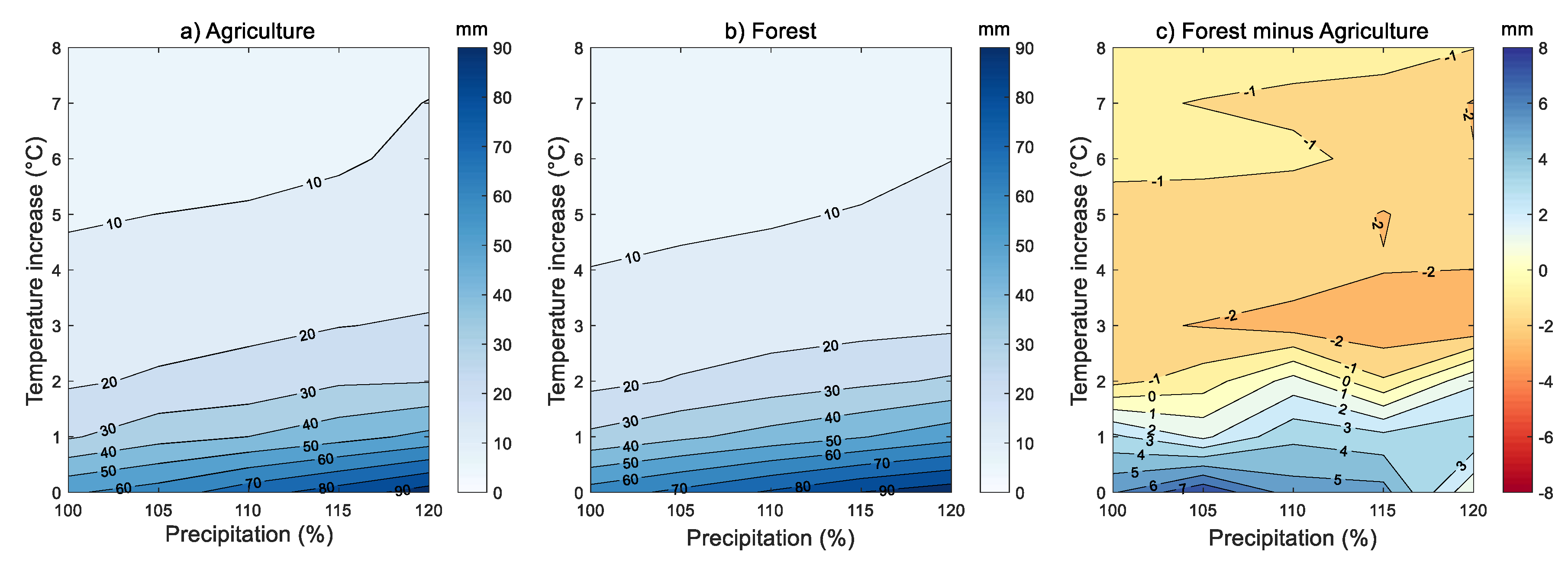
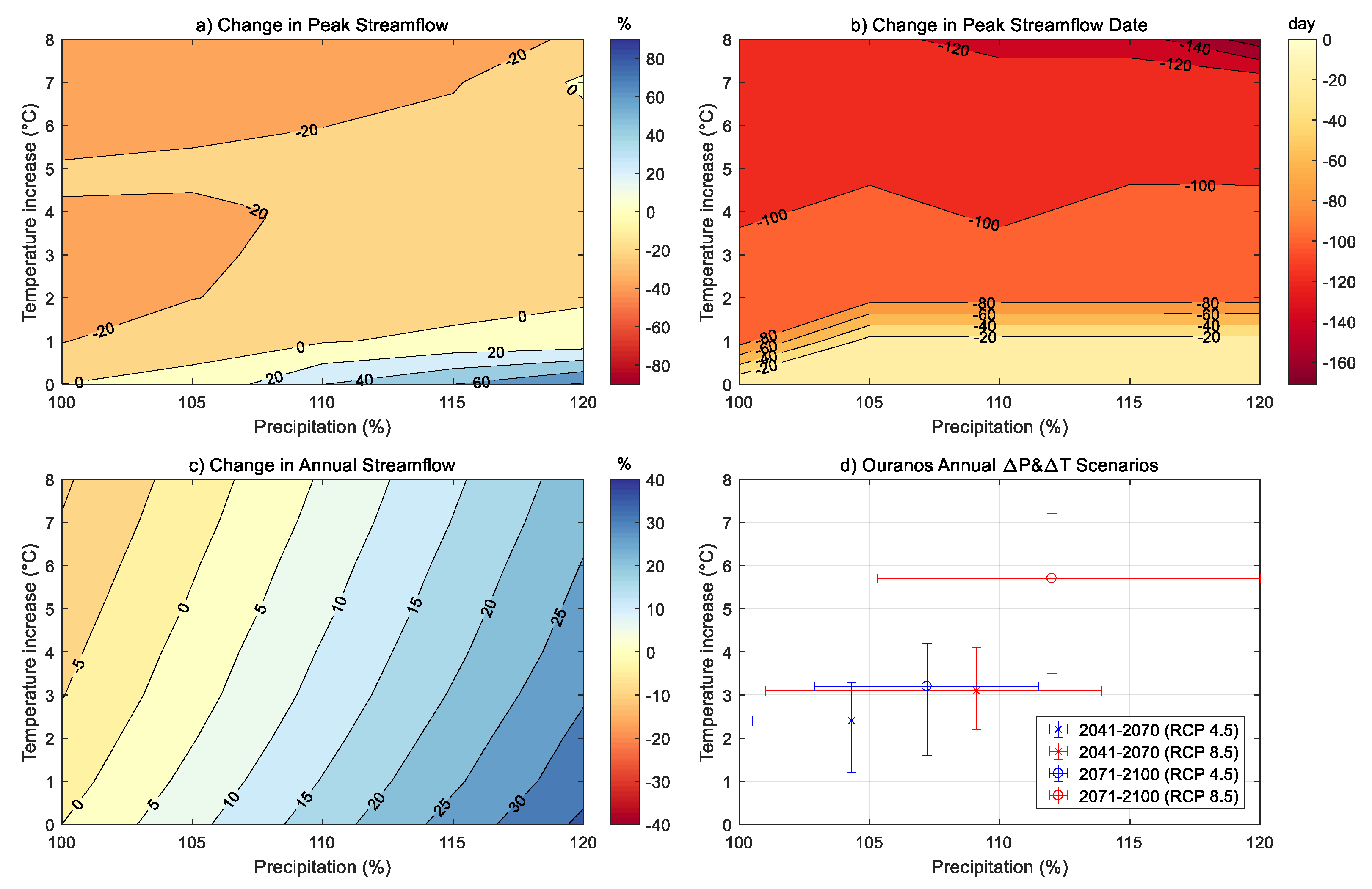
Table 1.
Modules used in the Cold Regions Hydrological Modelling (CRHM) platform to simulate the hydrological processes in the Acadie River Catchment.
Table 1.
Modules used in the Cold Regions Hydrological Modelling (CRHM) platform to simulate the hydrological processes in the Acadie River Catchment.
| CRHM Module | Description |
|---|---|
| Observation | Meteorological data are read and extrapolated with the environmental lapse rate. The phase of precipitation is predicted with a psychometric energy balance method using air temperature and relative humidity [73]. |
| Radiation | Calculates theoretical global radiation, direct and diffuse solar radiation, and maximum sunshine hours based on latitude, elevation, slope and azimuth [74]. |
| Sunshine hour | Sunshine hours are estimated from incoming short-wave radiation [75]. |
| Long-wave radiation | Estimates incoming long-wave radiation using observed short-wave radiation [76]. |
| All-wave radiation | The net all-wave radiation is calculated from short-wave radiation and the calculated net long-wave radiation [77] for snow-free conditions [78]. |
| Albedo | The snow albedo decay rate is calculated differently depending on the snow cover condition: pre-melt, melt, and post-melt. Albedo is estimated following a linear decay rate for each snow cover condition based on snow depth, new snow, and melting occurrence [79]. |
| Canopy | Estimates snowfall and rainfall intercepted by, and sublimated or evaporated from, forest canopy and unloaded or dripped from the canopy. It updates the under-canopy snowfall and rainfall and calculates short-wave and long-wave subcanopy radiation. This module has options for forest environments, small forest clearings, and open environments [18]. |
| Blowing snow transport | Simulates wind redistribution of snow and sublimation [21,34]. Wind redistribution depends on surface roughness, wind speed and atmospheric and snowpack conditions. |
| Snowpack energy-balance | The snowpack is represented by a two-layer mass and energy balance model (SNOBAL [80]). The energy balance includes net radiation, sensible and latent heat fluxes, ground heat, advection from rainfall, and change in internal energy. |
| Evapotranspiration | The Penman–Monteith algorithm [81] is used to calculate actual evapotranspiration from unsaturated surfaces and the Priestly–Taylor algorithm [82] is used for saturated surfaces. These algorithms access water from surface depression and soil moisture. |
| Crop growth | A linear crop development is simulated over the growing season, assuming the crops grow continuously from a prescribed Julian date to a maximum value [59]. Initial crop height at the beginning of the growing season, crop growth rate, crop planting date, crop maturity date and crop harvest date are used to estimate the crop height change over the growing season. These parameters are defined according to the most common crops (soya bean and corn) at the catchment using the studies performed in south west Québec [83,84]. |
| Infiltration | Snowmelt infiltration into frozen soil using a parametric equation [85] and rainfall infiltration into unfrozen soil based on soil texture and ground cover [86] are estimated. |
| Soil moisture | A three-layer model consists of two soil layers (recharge layer and lower layer) and a groundwater layer. It estimates soil moisture balance, depressional storage, surface/subsurface flows within two soil layers and groundwater discharge in the groundwater layer, and interactions between surface flow and groundwater [48,87,88]. The recharge (top) layer receives infiltration from depressional storage, snowmelt, and rainfall. Evaporation withdraws water first from canopy interception and depressional storage, whereas transpiration withdraws water from both soil layers depending on the rooting depth, soil moisture, stomata resistance and atmospheric conditions [89]. Horizontal and vertical flows from soil layers and groundwater layer are calculated based on Darcy’s law, where Brooks and Corey’s relationship [90] is used to estimate the actual hydraulic conductivity in the unsaturated zone. |
| Surface-subsurface runoff routing | Runoff between hydrological response units is routed using the Muskingum method based on the geometric characteristics of the stream channel [91]. Subsurface and groundwater flows are routed by Clark’s routing algorithm [92]. |
Table 2.
Sensitivity of snow variables to selected climate change scenarios. The snow onset date (SOD) and the snow disappearance date (SDD) are the first and last days of the water year with snow on the ground (SWE > 0.1 mm), respectively. SCD, snow cover duration.
Table 2.
Sensitivity of snow variables to selected climate change scenarios. The snow onset date (SOD) and the snow disappearance date (SDD) are the first and last days of the water year with snow on the ground (SWE > 0.1 mm), respectively. SCD, snow cover duration.
| Snow Variable | ΔT (°C) P (%) | 0 100 | 2 100 | 5 100 | 8 100 | 0 120 | 2 120 | 5 120 | 8 120 |
| Snowfall Ratio (%) | 23 | 17 | 11 | 8 | 23 | 17 | 11 | 8 | |
| Peak SWE (mm) | 65 | 19 | 9 | 5 | 100 | 32 | 13 | 7 | |
| SOD (DOWY *) | 20 | 45 | 45 | 58 | 20 | 26 | 45 | 58 | |
| Peak SWE Date (DOWY) | 148 | 140 | 83 | 77 | 148 | 140 | 83 | 77 | |
| SDD (DOWY) | 212 | 198 | 177 | 171 | 212 | 198 | 177 | 177 | |
| SCD (days) | 192 | 153 | 132 | 113 | 192 | 172 | 132 | 119 | |
| Snowmelt (mm year−1) | 201 | 145 | 99 | 67 | 251 | 180 | 121 | 82 | |
| Snowmelt Rate (mm day−1 year−1) | 1.04 | 0.95 | 0.75 | 0.59 | 1.31 | 1.05 | 0.91 | 0.68 | |
DOWY * = day of the water year (starting in 1 October).
Table 3.
Changes in magnitude of annual snow mass fluxes and resulting annual peak SWE in (a) agriculture and (b) forest under selected warming and increasing precipitation scenarios.
Table 3.
Changes in magnitude of annual snow mass fluxes and resulting annual peak SWE in (a) agriculture and (b) forest under selected warming and increasing precipitation scenarios.
| (a) Agriculture | ΔT (°C) P (%) | 0 100 | 2 100 | 5 100 | 8 100 | 0 120 | 2 120 | 5 120 | 8 120 |
| Drift out (mm year−1) | 4.5 | 2.2 | 0.6 | 0.2 | 5.0 | 2.7 | 0.8 | 0.3 | |
| Snowpack Sublimation (mm year−1) | 23.4 | 19.9 | 13.2 | 7.5 | 19.6 | 19.5 | 14.9 | 8.4 | |
| Blowing Snow Sublimation (mm year−1) | 10.3 | 5.2 | 1.5 | 0.5 | 11.5 | 6.4 | 2.1 | 0.6 | |
| Snowmelt (mm year−1) | 198 | 145 | 100 | 68 | 248 | 179 | 121 | 83 | |
| Sublimation Ratio (%) | 14.3 | 14.6 | 12.7 | 10.5 | 10.9 | 12.5 | 12.2 | 9.8 | |
| Drift Out Ratio (%) | 1.9 | 1.3 | 0.5 | 0.3 | 1.8 | 1.3 | 0.6 | 0.3 | |
| Snowmelt Ratio (%) | 83.8 | 84.2 | 86.7 | 89.2 | 87.3 | 86.2 | 87.2 | 89.9 | |
| Peak SWE (mm) | 59 | 19 | 9 | 5 | 95 | 30 | 13 | 7 | |
| (b) Forest | ΔT (°C) P (%) | 0 100 | 2 100 | 5 100 | 8 100 | 0 120 | 2 120 | 5 120 | 8 120 |
| Drift in (mm year−1) | 18.8 | 8.9 | 2.6 | 1.0 | 20.8 | 11 | 3.4 | 1.1 | |
| Snowpack Sublimation (mm year−1) | 22.6 | 18.6 | 12.7 | 6.3 | 18.8 | 18.8 | 13.5 | 7.2 | |
| Canopy Sublimation (mm year−1) | 23.8 | 18.6 | 13.2 | 9.1 | 19.2 | 14.5 | 17.5 | 19.1 | |
| Snowmelt (mm year−1) | 208 | 144 | 93 | 62 | 259 | 180 | 115 | 76 | |
| Sublimation Ratio (%) | 18.2 | 20.5 | 21.8 | 19.9 | 12.8 | 15.6 | 21.2 | 25.7 | |
| Snowmelt Ratio (%) | 81.8 | 79.5 | 78.2 | 80.1 | 87.2 | 84.4 | 78.8 | 74.3 | |
| Peak SWE (mm) | 65 | 17 | 8 | 5 | 96 | 31 | 12 | 6 | |
Table 4.
Mean annual catchment scale water fluxes for the selected climate change scenarios. For the reference period, the mean annual temperature is 7.2 °C and mean annual precipitation is 1030 mm.
Table 4.
Mean annual catchment scale water fluxes for the selected climate change scenarios. For the reference period, the mean annual temperature is 7.2 °C and mean annual precipitation is 1030 mm.
| Water Flux | ΔT (°C) P (%) | 0 100 | 2 100 | 5 100 | 0 120 | 2 120 | 5 120 |
| Rainfall Ratio (%) | 77 | 83 | 89 | 77 | 83 | 89 | |
| Annual Peak Streamflow (m3 s−1) | 19.3 | 14.8 | 15.9 | 35.3 | 19.0 | 18.2 | |
| Mean Winter Streamflow (m3 s−1) | 4.9 | 7.1 | 7.3 | 5.2 | 8.4 | 9.1 | |
| Mean Spring Streamflow (m3 s−1) | 9.5 | 6.9 | 6.1 | 13.2 | 9.3 | 8.0 | |
| Mean Summer Streamflow (m3 s−1) | 2.1 | 2.0 | 1.9 | 3.7 | 3.5 | 3.3 | |
| Evapotranspiration (mm year−1) | 462 | 479 | 497 | 479 | 498 | 520 | |
| Winter Snowmelt Infiltration (mm) (%) | 3.0 (4.2) | 2.6 (2.8) | 1.9 (2.5) | 2.8 (4.0) | 2.7 (2.4) | 3.5 (3.8) | |
| Winter Rainfall Infiltration (mm) (%) | 24 (33) | 39 (42) | 55 (45) | 24 (28) | 41 (37) | 60 (40) | |
| Spring Snowmelt Infiltration (mm) (%) | 4.4 (4) | 1.2 (3) | 0.7 (3.9) | 10 (6.4) | 1.0 (1.8) | 0.8 (3.5) | |
| Spring Rainfall Infiltration (mm) (%) | 107 (53) | 122 (55) | 131 (55) | 116 (47) | 134 (51) | 145 (51) | |
| Summer Infiltration (mm) (%) | 270 (94) | 272 (94) | 273 (95) | 307 (88) | 309 (89) | 311 (90) | |
| Groundwater Recharge (mm year−1) | 79 | 87 | 97 | 103 | 110 | 121 | |
| Winter Groundwater Recharge (mm) | 17 | 23 | 30 | 20 | 26 | 35 | |
| Surface Runoff Ratio * (%) | 43 | 33 | 24 | 40 | 32 | 23 | |
Surface runoff ratio * = The ratio of surface runoff volume to total streamflow volume.
Table 5.
Mean annual catchment scale water fluxes (falsified model) for the selected climate change scenarios.
Table 5.
Mean annual catchment scale water fluxes (falsified model) for the selected climate change scenarios.
| Water Flux | ΔT (°C) P (%) | 0 100 | 2 100 | 5 100 |
| Streamflow (mm year−1) | 414 | 408 | 400 | |
| Surface Runoff (mm year−1) | 13 | 12 | 11 | |
| Surface Runoff Ratio (%) | 3.2 | 2.9 | 2.8 | |
| Annual Peak Streamflow (m3 s−1) | 16 | 11.1 | 13 | |
© 2020 by the authors. Licensee MDPI, Basel, Switzerland. This article is an open access article distributed under the terms and conditions of the Creative Commons Attribution (CC BY) license (http://creativecommons.org/licenses/by/4.0/).
Share and Cite
MDPI and ACS Style
Aygün, O.; Kinnard, C.; Campeau, S.; Krogh, S.A. Shifting Hydrological Processes in a Canadian Agroforested Catchment due to a Warmer and Wetter Climate. Water 2020, 12, 739. https://doi.org/10.3390/w12030739
AMA Style
Aygün O, Kinnard C, Campeau S, Krogh SA. Shifting Hydrological Processes in a Canadian Agroforested Catchment due to a Warmer and Wetter Climate. Water. 2020; 12(3):739. https://doi.org/10.3390/w12030739
Chicago/Turabian StyleAygün, Okan, Christophe Kinnard, Stéphane Campeau, and Sebastian A. Krogh. 2020. "Shifting Hydrological Processes in a Canadian Agroforested Catchment due to a Warmer and Wetter Climate" Water 12, no. 3: 739. https://doi.org/10.3390/w12030739
Note that from the first issue of 2016, this journal uses article numbers instead of page numbers. See further details here.