Use of Global Sensitivity and Data-Worth Analysis for an Efficient Estimation of Soil Hydraulic Properties

Abstract

Accurate simulation of flow and contaminant transport processes through unsaturated soils requires adequate knowledge of the soil parameters. This study deals with the hydraulic characterization of soils using laboratory experiments. A new strategy is developed by combining global sensitivity analysis (GSA) and Bayesian data-worth analysis (DWA) to obtain efficient data that ensure a good estimation of the soil properties. The strategy is applied for the estimation of soil properties from a laboratory infiltration experiment. Results of this study show that GSA allows identification of regions and periods of high sensitivity of each parameter and thereby, the observations prone to contain information for a successful calibration. Further, the sensitivity depicts a nonlinear behavior with regions of high influence and regions of weak influence inside the parameter space. Bayesian DWA, performed a priori, allows to quantify the improvement of the posterior uncertainty of the estimated parameters when adding a type of measurement. The results reveal that an accurate estimation of the soil properties can be obtained if the target parameter values are located in the regions of high influence in the parameter space.

1. Introduction

Numerical models are essential tools for understanding the flow process through unsaturated soils, estimating subsurface recharge and/or prevent soil or water contamination. Application of numerical tools in field studies requires an adequate knowledge of the soil parameters. Some of the hydraulic parameters cannot be directly measured and inversion methods are usually applied to estimate these parameters. Generally, undisturbed soil samples are extracted in situ and taken to the laboratory where dynamic flow experiments can be performed under controlled conditions. The soil parameters are then estimated by fitting model outputs to the laboratory observations.

In the literature, several kinds of dynamic flow experiments, using different types of observations have been conducted to estimate the soil parameters. Among these experiments, one can mention one-step [1,2] and multistep [3,4,5,6,7] outflow experiments, infiltration experiments [8,9], extended multistep-outflow experiments [10], evaporation experiments [11,12], combined multistep-outflow and evaporation experiments [13], unsaturated transport experiments [14,15,16,17], and hydrogeophysical experiments [18,19].

Laboratory experiments are often time consuming, expensive, and tricky because of the risk of non-identifiability of the accepted parameters which depends on the measured data. Global sensitivity analysis (GSA) has been employed by Younes et al., [7] to help assess unsaturated soil hydraulic parameters. The GSA evaluates how output uncertainties are related to input parameter uncertainties with all the variation of inputs. In the last decades, GSA has been largely used for unsaturated flow in porous media. For instance, in Pan et al. [20], GSA has been conducted to assess the relative contribution of parameter uncertainties to the flow and transport uncertainties in a layered heterogeneous system. Brunetti et al. [21] used GSA to investigate the influence of soil hydraulic parameters on the behavior of a permeable pavement. Younes et al. [19] used GSA to investigate the influence of hydraulic and geophysical parameters on the streaming potential signals. In van Griensven et al. [22], GSA has been used to reduce the number of parameters and thus reduce over-parametrization of the numerical model.

GSA allows to quantify the impact changes of parameters have on the model output. By this way, GSA enables the detection of the important parameters, their regions, and periods of influence [23]. This can facilitate the experimental procedure by identifying strategic measurements that could be relevant for soil characterization. However, collecting new output observations even when the output is highly sensitive to the parameters may not reduce parameter uncertainties if the information contained in the new observations are already contained in the previous observations or in the case of parameter interactions. Hence, it is important to estimate the benefit of collecting new output observations (which may be costly) on the accuracy of the target parameters before collecting them.

This key point is addressed in this work by combining (GSA) with data worth analysis (DWA) to select efficient data for the characterization of the model parameters. This new strategy is applied for the estimation of hydraulic soil parameters from an infiltration laboratory experiment. The latter is carried out by injecting water at the top of an undisturbed sandy soil column. Richards equation, combined with the Mualem and van Genuchten (MvG) constitutive relationships [24,25], is employed to model the flow process. The unknown parameters are $K_s$ [L.T⁻¹], the saturated hydraulic conductivity; ${\theta }_r$ [L³.L⁻³], the residual water content; and $\alpha$ [L⁻¹] and $n$ [−], the MvG shape parameters. A first estimation of the soil parameters is carried out using cumulative outflow measurements. The interest of collecting tensiometric data and the best location of pressure sensors are then investigated by (i) analysis of the pressure sensitivity to the hydraulic soil parameters at different locations using GSA and (ii) performing a Bayesian DWA to quantify the benefit of the pressure head measurements on reducing posterior parameter uncertainty intervals, and thereby, improving the quality of the estimated parameters.

In this work, GSA is conducted using Polynomial Chaos Expansion [23,26] to explore the variance-based sensitivity indices [27,28]. These indices measure how each parameter affects the model output variance [29]. The Sobol’ indices are well suited for hydrologic models since they do not require linearity or monotony of the model. DWA is performed using Bayesian parameter inference via Markov Chain Monte Carlo (MCMC) method. Bayesian estimation methods are increasingly used since they combine prior parameters information with observations to provide posterior parameter distributions from which many statistics can be calculated [30]. The MCMC sampler randomly generates values of parameters from the joint probability density functions, using the Metropolis-Hastings algorithm [31,32]. The MCMC method is preferred over the gradient-based local optimization algorithms, which may fail to provide reliable confidence intervals [19,33,34,35].

2. Materials and Methods

2.1. Laboratory Experiment

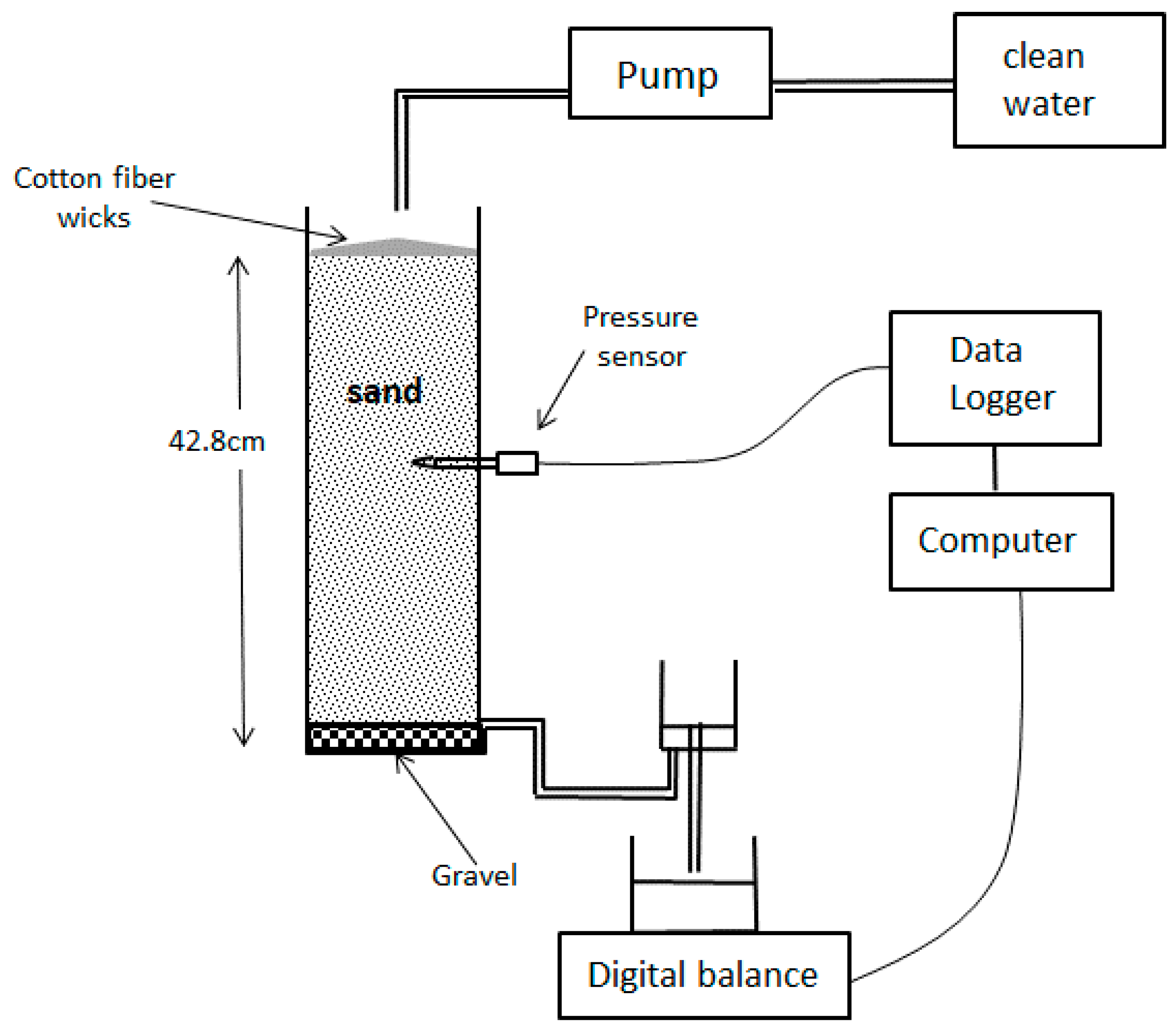
A PVC tube of 55 cm length was used for the extraction of an undisturbed soil column of 42.8 cm in the region of Bekalta in the East-Center of Tunisia. The soil was made up of approximately 93% sand, 5% silt and 2% clay particles. Figure 1 shows the experimental setup, where a column was filled with the undisturbed soil. A small container, filled with gravel was fixed at the bottom in order to maintain a fixed zero pressure as a lower boundary condition. Water was injected at the soil surface with a constant rate of 0.115 cm/min using an accurate peristaltic pump. Cotton fiber wicks were set at the soil surface to allow lateral distribution of water and hence ensure a one-dimensional vertical flow. The injection of water occurred between t = 17 min and t = 75.5 min. The cumulative outflow was monitored until t = 118 min. The initial pressure distribution was the correspondent to a hydrostatic distribution. A Neumann boundary condition was used at the top, with a constant injection flow $q_{inj}$ of 0.115 cm/min over the entire injection period $\left(17\hspace{0.17em}\hspace{0.17em}\min <t<75.5\hspace{0.17em}\min \right)$, else $q_{inj}=0$. A Dirichlet boundary condition was maintained at the bottom with zero prescribed pressure.

An accurate digital balance was used to monitor the cumulative outflow. The benefit of using a pressure sensor as well as its position inside the soil column will be investigated for the following depths: 18.5 cm, 23.5 cm, and 33 cm from the soil surface.

2.2. Numerical Model

The Richards Equation (RE) governed the flow through the unsaturated one-dimensional undisturbed soil column:

$$\{\begin{array}{l}\frac{\partial \theta }{\partial t}=\left(C_s\left(h\right)+S_s\frac{\theta }{{\theta }_S}\right)\frac{\partial h}{\partial t}=-\frac{\partial q_d}{\partial z}\\ \hspace{0.17em}\hspace{0.17em}{q}_d=-K\left(h\right)\left(\frac{\partial h}{\partial z}-1\right)\end{array}$$

(1)

where $\theta$ [L³.L⁻³], the current water content; t [T⁻¹], the time; $c\left(h\right)$ [L⁻¹], the specific moisture capacity; $S_s$ [L⁻¹], the specific storage; ${\theta }_s$ [L³.L⁻³], the saturated water content; $q$ [L.T⁻¹], the Darcy’s velocity; z [L], the positive downward vertical coordinate and $K\left(h\right)$ [L.T⁻¹], the hydraulic conductivity. The models of Mualem [24] and van Genuchten [25] were used for water content – pressure head, and conductivity – water content constitutive relationships as follows:

$$\begin{array}{l}{S}_e\left(h\right)=\frac{\theta \left(h\right)-{\theta }_r}{{\theta }_s-{\theta }_r}=\{\begin{array}{ll}\frac{1}{{\left(1+{\left|\alpha h\right|}^n\right)}^m}& h<0\\ 1& h\ge 0\end{array}\\ K\left(S_e\right)=K_s{S}_e{}^{1/2}{\left[1-{\left(1-S_e{}^{1/m}\right)}^m\right]}^2\end{array}$$

(2)

where $m=1-1/n$ and S_e (-) is the effective saturation.

The finite volume method was used to solve the problem given by Equations (1) and (2), with a uniform discretization containing 214 cells of a uniform size of 0.2 cm. This fine discretization yielded a mesh independent solution. The time solver DLSODIS [36] was used for an efficient time discretization. This solver used the method of lines (MOL), which allowed variable-order time integration and variable time step size while controlling the temporal error [37]. Note that, the MOL method works well with the nonlinear Richards Equation (RE) [38] and provides a mass conservative solution for its h form [39]

2.3. Global Sensitivity Analysis

Global sensitivity analysis is generally employed to assess the role of a parameter in the model output variance [40], which allows detecting influential parameters and irrelevant parameters. A parameter is considered irrelevant if its variation does not affect the output of the model. Such a parameter cannot be identified from the output measurements. Further, GSA enables the detection of the most important parameters, their regions, and periods of influence. This can help in selecting the position where sensors should be located, and the time when special attention should be paid when monitoring the model outputs.

In this study, the variance-based sensitivity indices were employed for the GSA. These indices reflect the contribution of each parameter to the variance of the model output [29]. The Sobol’ indices were evaluated using a surrogate model approach based on Polynomial Chaos Expansion (PCE) [26,41,42,43,44].

Let us consider a random mathematical model $f\left(\mathsf{\xi }\right)$ depending on $d$ independent random parameters $\mathsf{\xi }=\left\{{\xi }_1,{\xi }_2,\dots ,{\xi }_d\right\}$. With PCE, the random model response $f\left(\mathsf{\xi }\right)$ is expanded up to a polynomial degree p as follows:

$$f\left(\mathsf{\xi }\right)\approx {\displaystyle \sum _{\left|\alpha \right|\le p}{C}_{\alpha }{\mathsf{\Psi }}_{\alpha }}$$

(3)

where $\alpha ={\alpha }_1\dots {\alpha }_d\in {ℝ}^d$ is a d^th-dimensional index, $C_{\alpha }$ are the polynomial coefficients, and ${\mathsf{\Psi }}_{\alpha }$ are the multivariate orthonormal polynomials of degree $\left|\alpha \right|={\displaystyle {\sum }_{i=1}^d{\alpha }_i}$. Multivariate orthonormal polynomials are a tensor-product of univariate polynomials [45]. The Legendre polynomials, with non-informative uniform distributions, were used in this work for all parameters. These distributions express the lack of prior information on the parameter values, which renders all plausible values equally likely.

From Equation (3), the variance $V\left[f\left(\mathsf{\xi }\right)\right]$ writes,

$$V\left[f\left(\mathsf{\xi }\right)\right]={\displaystyle \sum _{\alpha }{C}_{\alpha }^2}$$

(4)

The Sobol’ first-order index $S_i$ measures the contribution of ${\xi }_i$ alone to the variance of the model response $f\left(\mathsf{\xi }\right)$

$$S_i=\frac{V\left[E\left[f\left(\mathsf{\xi }\right)|{\xi }_i\right]\right]}{V\left[f\left(\mathsf{\xi }\right)\right]}\in \left[0,1\right]$$

(5)

The total sensitivity index $S{T}_i\ge S_i$, measures the part of the model response $f\left(\mathsf{\xi }\right)$ due to all the contributions of ${\xi }_i$ (including the non-linear interaction between ${\xi }_i$ and the parameters ${\xi }_j$) with ${\mathsf{\xi }}_{-i}=\mathsf{\xi }\backslash {\xi }_i$, $E\left[\left(.|.\right)\right]$, the conditional expectation operator and $V\left[\left(.|.\right)\right]$, the conditional variance.

$$S{T}_i=\frac{E\left[V\left[f\left(\mathsf{\xi }\right)|{\mathsf{\xi }}_{-i}\right]\right]}{V\left[f\left(\mathsf{\xi }\right)\right]}\in \left[0,1\right]$$

(6)

The input/output relationship is called additive if $S{T}_i=S_i,\hspace{0.17em}\forall \hspace{0.17em}i=1,\mathrm{..},d$ and in this case, ${\displaystyle {\sum }_{i=1}^d{S}_i}=1$ The surrogate PCE model has $P=\frac{\left(d+p\right)!}{d!p!}$ coefficients. The evaluation of these coefficients requires at least P simulations of the direct model.

2.4. Bayesian Parameter Inference

The value of ${\theta }_s$ was fixed at 0.42 cm³.cm⁻³. This value has been accurately obtained by weighing a sample of the saturated soil. The specific storage was fixed at 5E10⁻⁹ cm⁻¹. Therefore, the unknowns vector reduced to $\mathsf{\xi }=\left(K_S,\hspace{0.17em}{\theta }_r,\alpha ,n\right)$. This vector was estimated using a Bayesian inversion to obtain the joint posterior probability distribution functions (jpdfs). These functions were evaluated using the DREAM_(ZS) [46] MCMC sampler, which was largely used in sub-surface hydrology e.g., [9,15,16,46,47,48]. DREAM_(ZS) generates random parameter set sequences which converge asymptotically to the target solution [49]. Statistical measures, such as the mean or the variance, are calculated from the obtained posterior distributions. All parameters were assumed to have uniform distributions over their respective intervals shown in

Table 1. Prior intervals of the hydraulic soil parameters.

Parameter	Lower Bound	Upper Bound
$K_S$ [cm/min]	0.10	2.0
${\theta }_r$ [-]	0.05	0.15
$\alpha$ [cm−1]	0.005	0.15
$n$ [-]	1.5	13.

. As little is known about the model parameters, these large intervals were based on the literature.

The Metropolis–Hastings algorithm employed in MCMC uses a probability distribution to generate a sequence of random samples. At the ith iteration, the algorithm generates a new candidate ${\mathsf{\xi }}^i$, from a distribution $q\left({\mathsf{\xi }}^i|{\mathsf{\xi }}^{i-1}\right)$ depending only on the accepted candidate. Then, ${\mathsf{\xi }}^i$ can be rejected or accepted depending on the following Hasting ratio ${\alpha }_H$,

$${\alpha }_H=min\left(1,\frac{p\left({\mathsf{\xi }}^i|{\mathrm{y}}_{mes}\right)q\left({\mathsf{\xi }}^i|{\mathsf{\xi }}^{i-1}\right)}{p\left({\mathsf{\xi }}^{i-1}|{\mathrm{y}}_{mes}\right)q\left({\mathsf{\xi }}^{i-1}|{\mathsf{\xi }}^i\right)}\right)$$

(7)

In this work, DREAM_(ZS) was used with three parallel chains. We considered that convergence aws reached if the chains were not correlated and the Gelman- Rubin [50] criterion was fulfilled $\left(R_{stat}\le 1.2\right)$. The last 25% parameter sets (after convergence of the chains) were used for the estimation of the mean parameter values and the corresponding confidence intervals.

3. Results and Discussion

3.1. Inversion Using Cumulative Outflow Measurements

This section shows the results of hydraulic parameter estimation by fitting the cumulative outflow measurements. These measurements were obtained using an accurate digital balance, as described above.

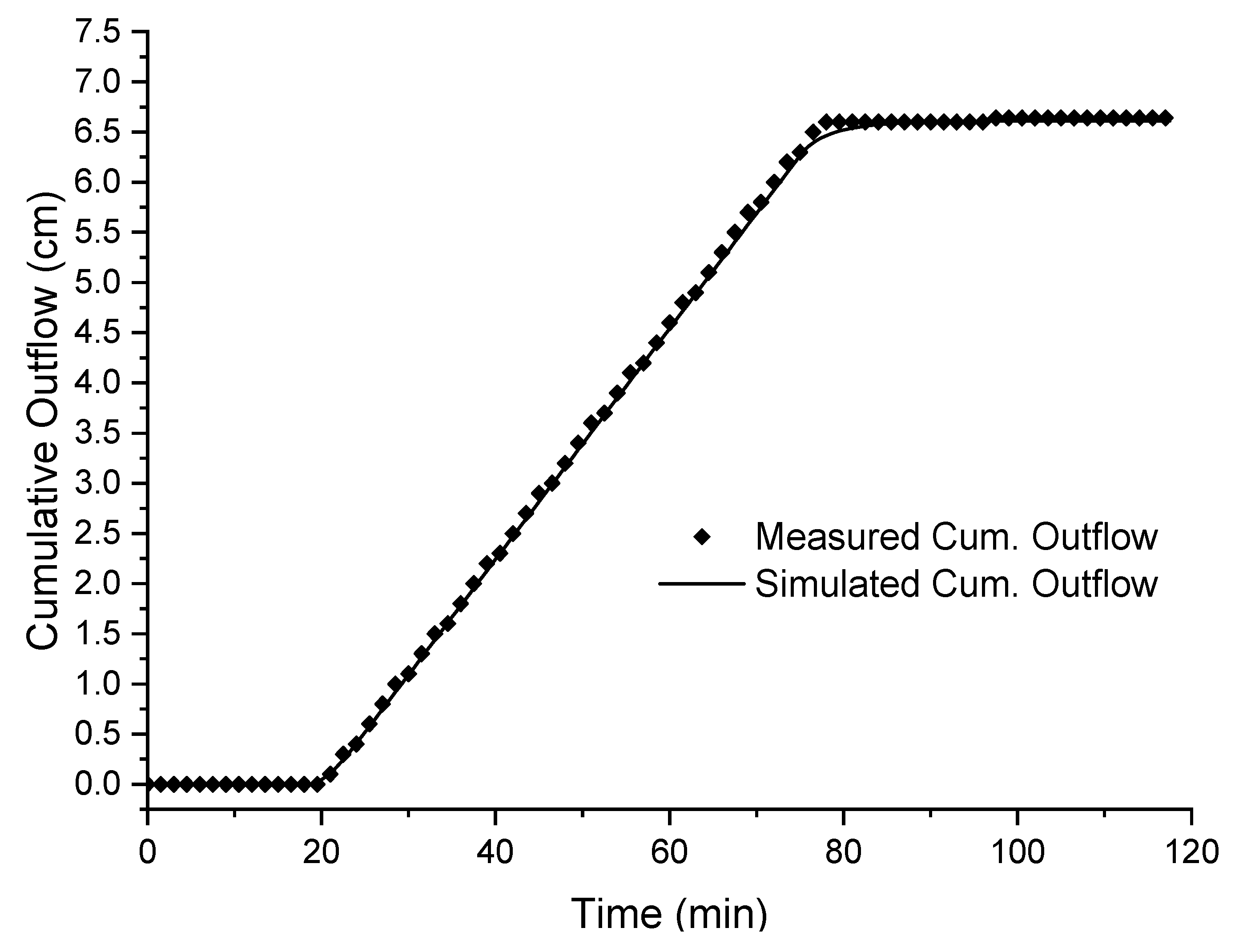
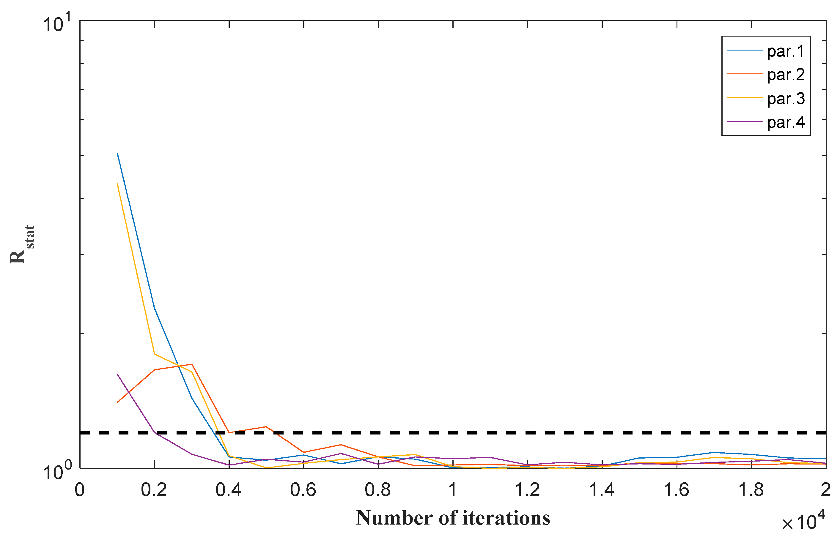
Figure 2 compares measured and simulated cumulative outflow using estimated parameter values. In this figure, the cumulative outflow depicts a linear behavior during the injection period. The calibrated curve fit the measurements of cumulative outflow very well. As shown in Figure 3, the overall chains converged after 6000 model runs. The results of the inversion using MCMC are shown in

Table 2. Mean parameter values, confidence intervals (Cis) and size of the CIs when only cumulative outflow observations are used for parameter calibration.

	Unit	Mean Value	99% Confidence Interval	Size of the 99% Confidence Interval
$K_S$	(cm/min)	1.37	[0.1–2.0]	1.9
${\theta }_r$	-	0.104	[0.05–0.15]	0.1
$\alpha$	(cm−1)	0.019	[0.01–0.029]	0.028
$n$	-	2.19	[0.6–3.8]	3.2

which includes the mean parameter values and the 99% confidence intervals (CIs).

The results shown in Table 2 reveal that $K_S$ and ${\theta }_r$ could not be identified using only the cumulative outflow observations as no reduction of their intervals of variation was observed (their posterior CIs were similar to their prior intervals of variation given in Table 1). The van Genuchten shape parameters $\alpha$ and n were better estimated since their posterior CIs were respectively six times and three times smaller than their prior intervals of variation. Their CIs remained, however, quite large (Table 2). Note that van Dam et al. [3] conducted a multistep outflow experiment and showed that the three parameters $\left({\theta }_r, \alpha , n\right)$ can be well identified from the cumulative outflow observations. However, Younes et al. [7], conducted a percolation drainage experiment and showed that cumulative outflow measurements could be sufficient for the estimation of the soil parameters only for some kinds of soils. Further, Younes et al. [7] found that in the case of a percolation-drainage experiment, the inverse solution can be greatly improved when cumulative outflow data are supplemented with simultaneous measure of pressure head. Hence, we investigate hereafter, the utility and benefit of using tensiometers for monitoring the pressure head at different depths in the soil column in the case of infiltration experiment. For this purpose, and before installing tensiometers, the impact of pressure data on posterior parameter uncertainty intervals was investigated using GSA and DWA.

3.2. Global Sensitivty Analysis Results

GSA was performed using a PCE of order 4 for each location and observable time. The PCEs contained 70 coefficients each and were calculated using the regression method [23]. Fitting the PCE results to the RE pressure head responses was done for a random experimental design formed by 100 parameter sets. The pressure head responses were analyzed at 18.5 cm, 23.5 cm, and 33 cm from the soil surface. It was assumed that the four soil parameters $\left(K_S,\hspace{0.17em}{\theta }_r,\alpha ,n\right)$ were uniformly distributed within the posterior 99% Confidence Intervals (CIs) obtained in Table 2.

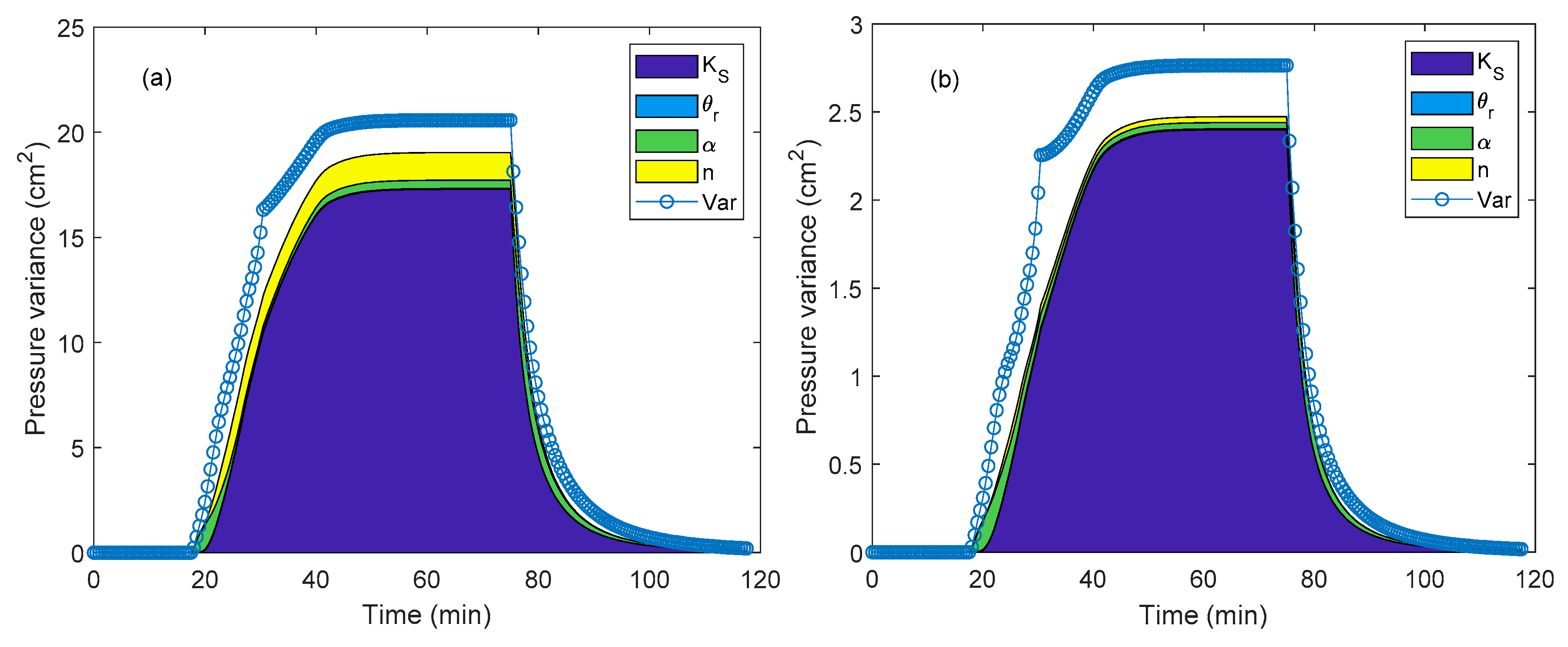
The results of GSA showed that the pressure variance as well as the contribution of each parameter to that variance had a similar behavior for the three investigated locations. Figure 4 depicts the pressure head variance (blue curve) versus time at $z_1=18.5$ cm (Figure 4a) and $z_3=33$ cm (Figure 4b) from the soil surface. In this figure, the shaded areas represent the amount of variance due to each parameter alone. Interaction between parameters is represented by the blank region below the variance curve and above the shaded area. As shown in this figure, the pressure variance was zero at the beginning since the infiltration water front did not yet reach the pressure sensor. Then, it increased to reach a stable value, and finally, it decreased when infiltration was stopped. Towards the end of the experiment, the variance reduced to zero since the flow becames negligible after 100 min, regardless of the parameter set.

In both graphs of Figure 4, the most influential parameters are $K_S$ and then $n$. The parameter $\alpha$ had a smaller effect on the pressure head. Note that Younes et al. [7] found that for the percolation drainage experiment, the sensitivity of the pressure head to $\alpha$ is higher than to $n$. This shows that the sensitivity of an output to a parameter depends on the investigated soil and on the type of boundary conditions. The results of Figure 4 show that the residual water content was not relevant as no effect was observed on the three investigated pressure heads. Similar results were obtained by Younes et al. [7] in the case of percolation drainage experiment.

The comparison between the graphs 4a and 4b shows that a similar behavior was observed for the two pressure locations. However, the variance of the pressure was around 10 times more significant in the Figure 4a. Besides, the relative importance of $\alpha$ and $n$ to the pressure variance was more pronounced at $z_1=18.5$ cm than at $z_3=33$ cm. Furthermore, less interaction was observed between the investigated parameters in the Figure 4a. All these points suggest that the pressure at $z_1$ was more sensitive to the hydraulic parameters than at Z₃. This makes sense since the pressure head at $z_3$ had a reduced sensitivity to the soil parameters because of its vicinity with the lower boundary which had a zero pressure fixed during the whole experiment.

The obtained results show that:

(i)

The pressure head prediction was driven by hydraulic parameters and thus, the accuracy of the soil parameters may improve if the pressure data are also considered for calibration.

(ii)

If one has to install a single tensiometric sensor for collecting pressure head measurements, it is better to install it near the soil surface (near the top of the column).

(iii)

The parameter ${\theta }_r$ cannot be estimated from the pressure head measurements regardless to the position of the tensiometric sensor.

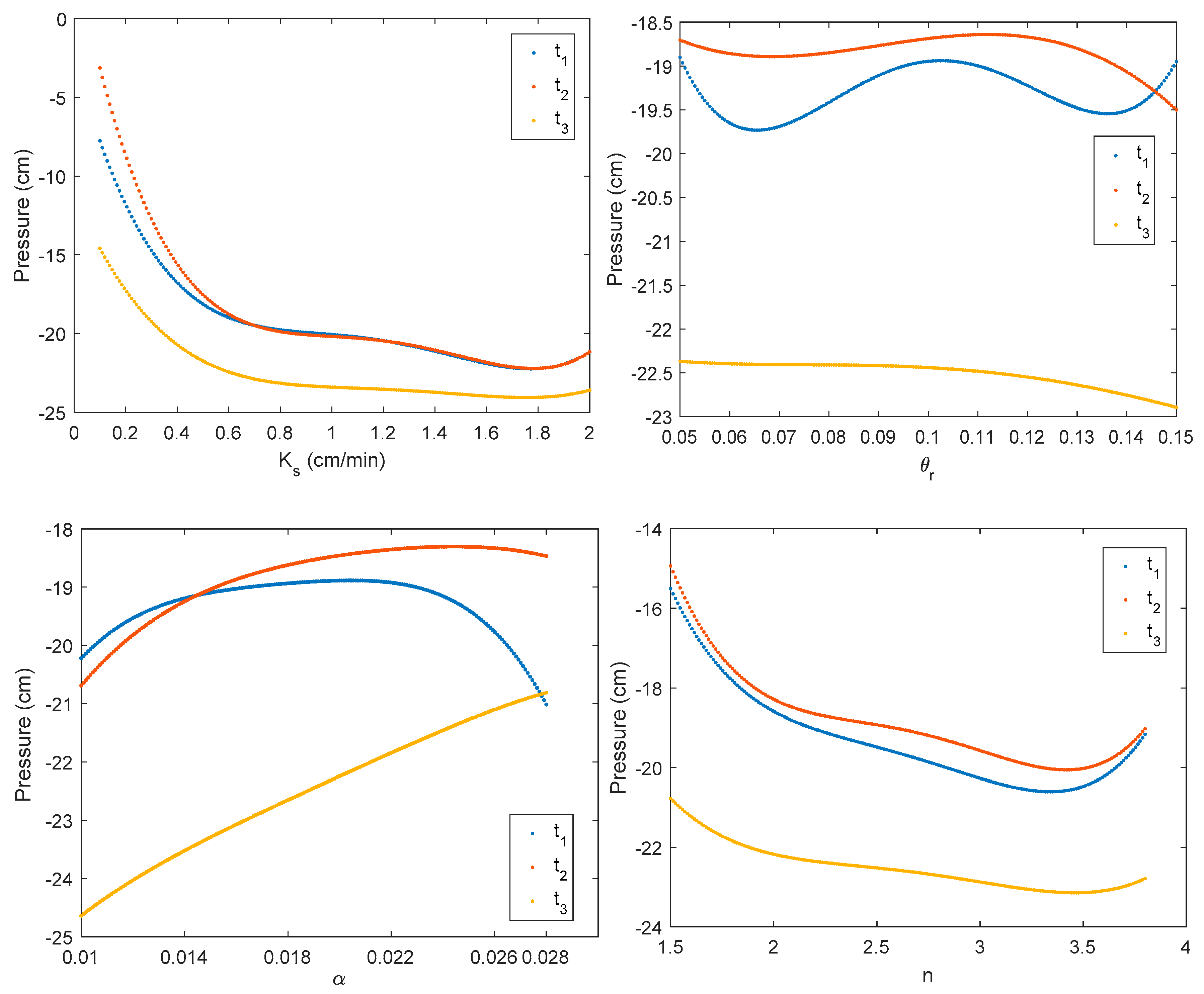
Recall that from the GSA results, a parameter is sensitive if the model output undergoes a significant variation for different plausible parameter values. However, the relationship between a parameter and the model output can be nonlinear. Thereby, the interval of variation of the parameter may contain regions of high influence (different values of the parameter taken in these regions yield strong variations of the model output) and regions of weak influence (different values of the parameter taken in these regions yield small variations of the model output). The Sobol’ indices (Figure 4) indicate the sensitivity of the parameters according to their whole intervals of variation, but do not give any information about regions of influence inside these intervals. To investigate these regions, the PCE used in GSA was employed to analyze the marginal effect of each parameter on the model output. This effect was investigated by analyzing the variation of the model output with respect to the chosen parameter whereas the other parameters are fixed at their mean values.

The marginal effects of the hydraulic parameters on the pressure head at 18.5 cm are shown in the Figure 5 for the following times: t₁ = 30 min which corresponds to the imbibition process, t₂ = 60 min which corresponds to the steady-state infiltration and t₃ = 80 min which corresponds to the drying process.

Figure 5 shows that $K_S$ had a significant effect on the pressure (significant negative slope) if its value was less than 0.6 cm/min, whereas, a weak sensitivity was observed for higher values. This implies that if pressure observations are used for the estimation of $K_S$, a more accurate estimation is expected if the target value is located inside the region of high influence ($K_S\le 0.6$ cm/min). The marginal effect of ${\theta }_r$ shows a nearly flat evolution (the pressure variation is less than 1 cm) at the three investigated times, which indicates that ${\theta }_r$ cannot be estimated using pressure data regardless of its target value. The marginal effect of $\alpha$ shows a significant impact on the whole parameter interval, which implies that $\alpha$ could be accurately estimated whatever its target value. Finally, the marginal effect of the parameter $n$ shows a high influence region (significant negative slope) for $n\le 3$, else its effect on the pressure value is weak. These results are similar to those obtained by Younes et al. [7] in the case of percolation-drainage experiment. In addition, the results of Figure 5 show that the sensitivity of the parameters $K_S$ and $n$ were more significant during the imbibition process (t₁), whereas, the parameter $\alpha$ was much more sensitive during the drying process (t₃).

3.3. Data Worth Analysis Results

The GSA allows to identify the regions and periods of influence for each parameter and hence, the observations prone to contain information and, thereby, that could be useful for the calibration. However, such analysis does not account for parameter interactions and redundancy of observations. Indeed, a parameter can be highly influential but not identifiable because of interactions between parameters. Furthermore, adding observations of a model output may not reduce the parameter uncertainty if the information contained in the new observations are already contained in the previous observations. Hence, it is important to estimate the benefit of collecting new output observations (which may be costly) on the accuracy of the target parameters before collecting them. In our case, to investigate the benefit of installing a tensiometric sensor for collecting pressure data at 18.5 cm, we proceeded as follows:

(i)

The numerical model was used to generate synthetic pressure head data at 18.5 cm using the mean parameter values obtained earlier from the calibration of the cumulative outflow data (Table 2, column 3).

(ii)

Then, the simulated pressure values were noised with Gaussian noises of 0.5 cm standard deviation and used as fictive new observations.

(iii)

The new fictive pressure observations were supplemented to the real cumulative outflow observations and used for a new Bayesian calibration of the hydraulic parameters.

Table 3. Mean parameter values, CIs and size of the posterior CIs when cumulative outflow observations and fictive pressure data are used for parameter assessment. The fictive pressure data are obtained from noised simulations performed using reference parameter values.

	Unit	Reference Value	Mean Value	99% Confidence Interval	Size of the 99% CI
$K_S$	(cm/min)	1.37	1.59	[0.9–2.3]	1.3
${\theta }_r$	-	0.104	0.106	[0.05–0.15]	0.1
$\alpha$	(cm−1)	0.0187	0.02	[0.017–0.025]	0.007
$n$	-	2.19	2.19	[1.56–2.64]	1.08

shows the reference parameter values, which were used to generate fictive pressure data, and the results of the estimation using real outflow measurements and fictive pressure data.

The results presented in this table show that using fictive pressure data in addition to real outflow measurements significantly improved the accuracy of the hydraulic parameters. Comparing results of Table 2 and Table 3 shows that adding fictive pressure data enabled a reduction of the CIs of around 32% for $K_S$, 75% for $\alpha$ and 66% for $n$. As expected, the parameter ${\theta }_r$ remains not identified since it had a negligible effect on the pressure head.

It is worth noting that the reference parameter value for the parameter $n$, used to generate fictive pressure data, as 2.19. This value was located inside the high influence region of the parameter ($n\le 3$). This was also the case for the parameter $\alpha$ since its high influence region corresponds to its whole interval of variation (see Figure 4). However, the reference value for $K_S$ (1.37 cm/min) was located inside its weak influence region (Figure 4). A new analysis was performed using the previous reference values for all parameters except for $K_S$, which was now fixed to 0.2 cm/min (this value was located inside the high influence region as can be seen in Figure 4). This analysis was performed to investigate how parameter uncertainty reduces if the target value of $K_S$ was located inside its high influence region. Similar to the previous case, the simulated pressure values at 18.5 cm were noised with a standard deviation of 0.5 cm and supplemented to the real cumulative outflow observations for the calibration of the hydraulic parameters. The results are summarized in

Table 4. Mean parameter values, CIs and size of the CIs when cumulative outflow observations and fictive pressure data are used for parameter assessment. The fictive pressure data correspond to noised simulations performed using reference parameter values.

	Unit	Reference Value	Mean Value	99% Confidence Interval	Size of the 99% CI
$K_S$	(cm/min)	0.2	0.19	[0.18–0.2]	0.02
${\theta }_r$	-	0.104	0.07	[0.05–0.15]	0.1
$\alpha$	(cm−1)	0.0187	0.0132	[0.012–0.014]	0.002
$n$	-	2.19	2.64	[2.4–2.8]	0.4

.

The results of Table 4 show that $K_S$, $\alpha$ and $n$ were more accurately estimated then previously. Their CIs were reduced by a factor of 50 for $K_S$, and a factor of 3 for $\alpha$ and $n$. Hence, DWA results show that pressure data at 18.5 cm improve the accuracy of the estimated hydraulic parameters by reducing their posterior CIs. This fully justifies the installation of a tensiomeric sensor to collect the pressure head at 18.5 cm. Furthermore, the benefit of such measurements can be highly significant if the target parameter values are located inside their high regions of influence shown in Figure 5.

3.4. Inversion Using Real Cumulative Outflow and Pressure Measurements

According to the previous results, the experiment was reperformed by installing a tensiometric sensor at 18.5 cm from the top of the soil. Both cumulative outflow and pressure head were monitored during the experiment. The results of MCMC, based on real observations, are given in

Table 5. Mean parameter values, CIs and size of the CIs when both real cumulative outflow and pressure observations are used for parameter assessment.

	Unit	Mean Value	99% Confidence Interval	Size of the 99% CI
$K_S$	(cm/min)	0.231	[0.22–0.24]	0.022
${\theta }_r$	-	0.07	[0.05–0.15]	0.1
$\alpha$	(cm−1)	0.012	[0.01–0.013]	0.003
$n$	-	2.26	[2–2.5]	0.5

. As shown in this table, the estimated mean value of $K_S$ was 0.23 cm/min, which was located inside the region of high influence ($K_S\le 0.6$ cm/min) plotted in Figure 4. The estimated mean value of $n$ (2.26) was also located in its high region of influence ($n\le 3$). This explains the highly accurate results obtained for all hydraulic parameters, except for ${\theta }_r$. Comparing the results to those of Table 2, which were obtained using only cumulative outflow measurements, shows that when both real cumulative outflow and pressure head measurements are used (Table 5), the CI of $K_S$ was reduced by a factor of 80. For $\alpha$ and $n$, the factor of reduction is respectively 9 and 6.

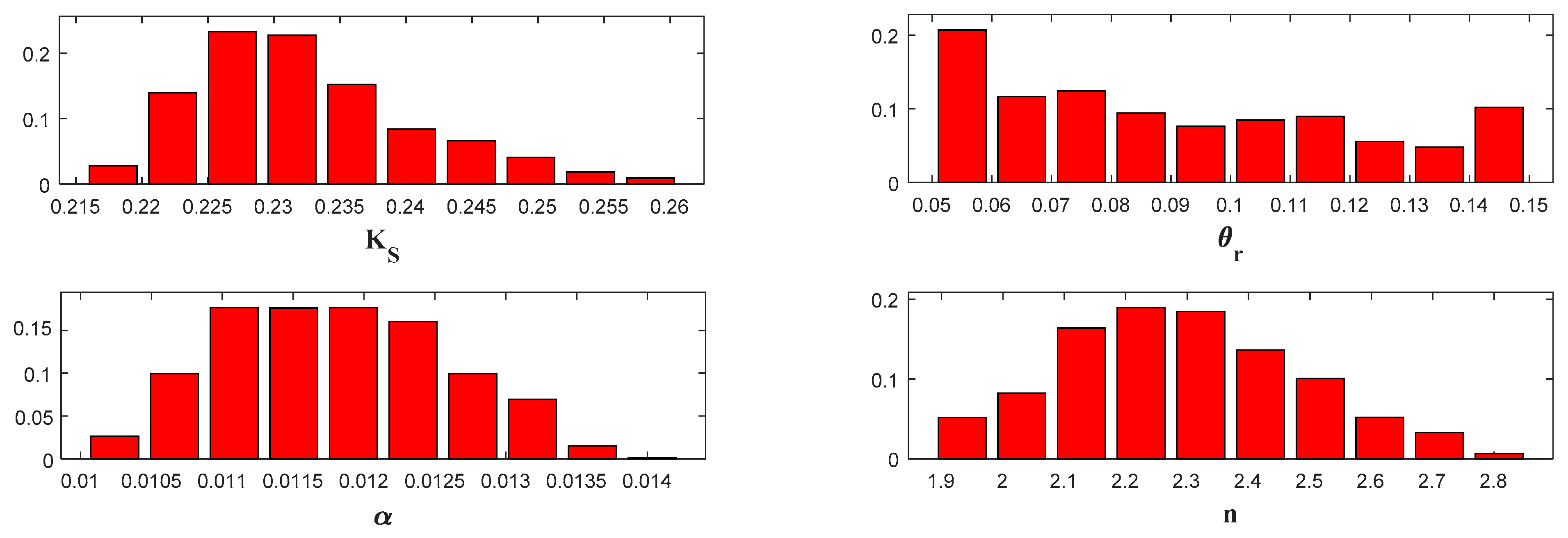
The MCMC sampler, in this case, converged in less than 10000 runs, and the posterior distributions for the parameters are plotted in Figure 6. As expected, the parameter ${\theta }_r$ could not be identified since its posterior distribution was almost uniform (similar to its prior one). The parameters $K_s$, $\alpha$ and $n$ were well estimated and had posterior bell-shaped distributions, which were significantly different from their prior uniform ones. This significant difference between prior and posterior distributions reflects the high sensitivity of the parameters. Moderate correlations are observed between $n$ and $K_s$ ($r=-0.92$), $\alpha$ and ${\theta }_r$ ($r=0.78$), and $n$ and $\alpha$ ($r=0.68$).

4. Conclusions

This study explored the possibility of determining the unsaturated hydraulic soil parameters using a laboratory infiltration experiment and GSA coupled with DWA. Bayesian parameter estimation was performed using MCMC. A first characterization of the soil parameters was conducted using the cumulative outflow measurements. These accurate and cheap observations did not allow identification of $K_S$ and ${\theta }_r$ and yielded large confidence intervals for $\alpha$ and n. This prompted us to investigate the benefits of installing tensiometric sensors for monitoring pressure head in the porous medium using GSA and DWA.

GSA of the pressure at three locations ($z_1=18.5$ cm, $z_2=23.5$ cm and $z_3=33$ cm) showed that the most sensitive parameters are K_s and then, the parameter n. The parameter ${\theta }_r$ does not affect the pressure at any of the three investigated positions. The results of GSA showed that it is better to collect the tensiometric data at $z_1=18.5$ cm since the pressure variance is around 10 times more significant than at $z_3=33$ cm. Further, the analysis of the marginal effects showed that $K_S$ and $n$ have a strong effect on the pressure head if $K_S\le 0.6$ cm/min, and $n\le 3$, else their effect on the pressure head is weak. $K_S$ and $n$ are more sensitive during the imbibition process, whereas, $\alpha$ is much more sensitive during the drying process.

The advantage of pressure measurements on the accuracy of the estimated parameters was investigated using fictive noised data stemming from simulations performed using parameter values obtained from the cumulative outflow calibration. Adding fictive pressure data enables a reduction of the CIs of around 32% for $K_S$, 75% for $\alpha$ and 66% for $n$. The parameter ${\theta }_r$ remains not identified since it has a negligible effect on the pressure. A second analysis showed that the accuracy of $K_S$ and $n$ can be improved if fictive pressure data were generated using parameter values located inside their high influence regions.

Finally, parameter estimation is carried out using real observations of pressure head and cumulative outflow. The estimated mean values of the parameters are located inside their regions of high influence. Compared to the results obtained using only cumulative outflow measurements, when both real cumulative outflow and pressure measurements are used, the CI of $K_S$ is reduced by a factor of 80. For $\alpha$ and $n$, the factor of reduction is respectively 9 and 6.

In summary, this study demonstrates the important role of GSA in the detection of, not only influential parameters, but also their regions and periods of high influence. This can help select the position where sensors should be located and the time when special attention should be paid for monitoring the model output. DWA can be used a priori to estimate the profit of adding a type of measurement on reducing parameter uncertainty intervals. This profit was shown to be highly significant if the target parameter values are located inside the high regions of influence of the parameters.

References

- Kool, J.B.; Parker, J.C.; van Genuchten, M.T. Determining Soil Hydraulic Properties from One-step Outflow Experiments by Parameter Estimation: I. Theory and Numerical Studies1. Soil Sci. Soc. Am. J. 1985, 49, 1348. [Google Scholar] [CrossRef] [Green Version]
- Parker, J.C.; Kool, J.B.; van Genuchten, M.T. Determining Soil Hydraulic Properties from One-step Outflow Experiments by Parameter Estimation: II. Experimental Studies1. Soil Sci. Soc. Am. J. 1985, 49, 1354. [Google Scholar] [CrossRef]
- Van Dam, J.C.; Stricker, J.N.M.; Droogers, P. Inverse method to determine soil hydraulic functions from multistep outflow experiments. Soil Sci. Soc. Am. J. 1994, 58, 647–652. [Google Scholar] [CrossRef]
- Durner, W.; Schultze, B.; Zurmühl, T. State-of-the-Art in Inverse Modeling of Inflow/Outflow Experiments; University of California: Riverside, CA, USA, 1999. [Google Scholar]
- Puhlmann, H.; Von Wilpert, K.; Lukes, M.; Dröge, W. Multistep outflow experiments to derive a soil hydraulic database for forest soils. Eur. J. Soil Sci. 2009, 60, 792–806. [Google Scholar] [CrossRef]
- Beydoun, H.; Lehmann, F. Expériences de drainage et estimation de paramètres en milieu poreux non saturé. Comptes Rendus Geosci. 2006, 338, 180–187. [Google Scholar] [CrossRef]
- Younes, A.; Mara, T.A.; Fajraoui, N.; Lehmann, F.; Belfort, B.; Beydoun, H. Use of Global Sensitivity Analysis to Help Assess Unsaturated Soil Hydraulic Parameters. Vadose Zone J. 2013, 12. [Google Scholar] [CrossRef]
- Mishra, S.; Parker, J.C. Parameter estimation for coupled unsaturated flow and transport. Water Resour. Res. 1989, 25, 385–396. [Google Scholar] [CrossRef]
- Younes, A.; Zaouali, J.; Fahs, M.; Slama, F.; Grunberger, O.; Mara, T.A. Bayesian soil parameter estimation: Results of percolation-drainage vs. infiltration laboratory experiments. J. Hydrol. 2018, 565, 770–778. [Google Scholar] [CrossRef]
- Durner, W.; Iden, S.C. Extended multistep outflow method for the accurate determination of soil hydraulic properties near water saturation. Water Resour. Res. 2011, 47. [Google Scholar] [CrossRef] [Green Version]
- Wendroth, O.; Ehlers, W.; Hopmans, J.W.; Kage, H.; Halbertsma, J.; Wösten, J.H.M. Reevaluation of the evaporation method for determining hydraulic functions in unsaturated soils. Soil Sci. Soc. Am. J. 1993, 57, 1436–1443. [Google Scholar] [CrossRef]
- Kumar, S.; Sekhar, M.; Reddy, D.V.; Mohan Kumar, M.S. Estimation of soil hydraulic properties and their uncertainty: Comparison between laboratory and field experiment. Hydrol. Process. 2010, 24, 3426–3435. [Google Scholar] [CrossRef]
- Schelle, H.; Iden, S.C.; Durner, W. Combined transient method for determining soil hydraulic properties in a wide pressure head range. Soil Sci. Soc. Am. J. 2011, 75, 1681–1693. [Google Scholar] [CrossRef]
- Moreira, P.H.S.; van Genuchten, M.T.; Orlande, H.R.B.; Cotta, R.M. Bayesian estimation of the hydraulic and solute transport properties of a small-scale unsaturated soil column. J. Hydrol. Hydromech. 2016, 64, 30–44. [Google Scholar] [CrossRef] [Green Version]
- Younes, A.; Mara, T.; Fahs, M.; Grunberger, O.; Ackerer, P. Hydraulic and transport parameter assessment using column infiltration experiments. Hydrol. Earth Syst. Sci. 2017, 21, 2263–2275. [Google Scholar] [CrossRef] [Green Version]
- Younes, A.; Mara, T.A.; Voltz, M.; Guellouz, L.; Musa Baalousha, H.; Fahs, M. A new efficient Bayesian parameter inference strategy: Application to flow and pesticide transport through unsaturated porous media. J. Hydrol. 2018, 563, 887–899. [Google Scholar] [CrossRef]
- Younes, A.; Zaouali, J.; Kanzari, S.; Lehmann, F.; Fahs, M. Bayesian Simultaneous Estimation of Unsaturated Flow and Solute Transport Parameters from a Laboratory Infiltration Experiment. Water 2019, 11, 1660. [Google Scholar] [CrossRef] [Green Version]
- Mboh, C.M.; Huisman, J.A.; Zimmermann, E.; Vereecken, H. Coupled Hydrogeophysical Inversion of Streaming Potential Signals for Unsaturated Soil Hydraulic Properties. Vadose Zone J. 2012, 11. [Google Scholar] [CrossRef]
- Younes, A.; Zaouali, J.; Lehmann, F.; Fahs, M. Sensitivity and identifiability of hydraulic and geophysical parameters from streaming potential signals in unsaturated porous media. Hydrol. Earth Syst. Sci. 2018, 22, 3561–3574. [Google Scholar] [CrossRef] [Green Version]
- Pan, F.; Zhu, J.; Ye, M.; Pachepsky, Y.A.; Wu, Y.S. Sensitivity analysis of unsaturated flow and contaminant transport with correlated parameters. J. Hydrol. 2011, 397, 238–249. [Google Scholar] [CrossRef]
- Brunetti, G.; Šimůnek, J.; Turco, M.; Piro, P. On the use of global sensitivity analysis for the numerical analysis of permeable pavements. Urban Water J. 2018, 15, 269–275. [Google Scholar] [CrossRef] [Green Version]
- van Griensven, A.; Meixner, T.; Grunwald, S.; Bishop, T.; Diluzio, M.; Srinivasan, R. A global sensitivity analysis tool for the parameters of multi-variable catchment models. J. Hydrol. 2006, 324, 10–23. [Google Scholar] [CrossRef]
- Fajraoui, N.; Ramasomanana, F.; Younes, A.; Mara, T.A.; Ackerer, P.; Guadagnini, A. Use of global sensitivity analysis and polynomial chaos expansion for interpretation of nonreactive transport experiments in laboratory-scale porous media. Water Resour. Res. 2011, 47, W02521. [Google Scholar] [CrossRef]
- Mualem, Y. A new model for predicting the hydraulic conductivity of unsaturated porous media. Water Resour. Res. 1976, 12, 513–522. [Google Scholar] [CrossRef] [Green Version]
- van Genuchten, M.T. A Closed-form Equation for Predicting the Hydraulic Conductivity of Unsaturated Soils. Soil Sci. Soc. Am. J. 1980, 44, 892–898. [Google Scholar] [CrossRef] [Green Version]
- Sudret, B. Global sensitivity analysis using polynomial chaos expansions. Reliab. Eng. Syst. Saf. 2008, 964–979. [Google Scholar] [CrossRef]
- Homma, T.; Saltelli, A. Importance measures in global sensitivity analysis of nonlinear models. Reliab. Eng. Syst. Saf. 1996, 52, 1–17. [Google Scholar] [CrossRef]
- Sobol’, I.M. Sensitivity estimates for nonlinear mathematical models. Math. Model. Comput. Exp. 1993, 1, 407–414. [Google Scholar]
- Sobol′, I.M. Global sensitivity indices for nonlinear mathematical models and their Monte Carlo estimates. Math. Comput. Simul. 2001, 55, 271–280. [Google Scholar] [CrossRef]
- Kaipio, J.; Somersalo, E. Statistical and Computational Inverse Problems; Applied Mathematical Sciences; Springer: New York, NY, USA, 2004; p. 160. [Google Scholar]
- Hastings, W.K. Monte Carlo sampling methods using Markov chains and their applications. Biometrika 1970, 57, 97–109. [Google Scholar] [CrossRef]
- Metropolis, N.; Rosenbluth, A.W.; Rosenbluth, M.N.; Teller, A.H.; Teller, E. Equation of state calculations by fast computing machines. J. Chem. Phys. 1953, 21, 1087–1092. [Google Scholar] [CrossRef] [Green Version]
- Gallagher, M.; Doherty, J. Parameter estimation and uncertainty analysis for a watershed model. Environ. Model. Softw. 2007, 22, 1000–1020. [Google Scholar] [CrossRef]
- Kahl, G.M.; Sidorenko, Y.; Gottesbüren, B. Local and global inverse modelling strategies to estimate parameters for pesticide leaching from lysimeter studies: Inverse modelling to estimate pesticide leaching parameters from lysimeter studies. Pest Manag. Sci. 2015, 71, 616–631. [Google Scholar] [CrossRef] [PubMed]
- Vrugt, J.A.; Bouten, W. Validity of first-order approximations to describe parameter uncertainty in soil hydrologic models. Soil. Sci. Soc. Am. J. 2002, 66, 1740–1751. [Google Scholar] [CrossRef] [Green Version]
- Hindmarsh, A.C. LSODE and LSODI, two new initial value ordinary differential equation solvers. ACM Signum Newsl. 1980, 15, 10–11. [Google Scholar] [CrossRef]
- Miller, C.T.; Abhishek, C.; Farthing, M.W. A spatially and temporally adaptive solution of Richards’ equation. Adv. Water Resour. 2006, 29, 525–545. [Google Scholar] [CrossRef]
- Farthing, M.W.; and Ogden, F.L. Numerical solution of Richards’ equation: A review of advances and challenges. Soil Sci. Soc. Am. J. 2017, 81, 1257–1269. [Google Scholar] [CrossRef] [Green Version]
- Fahs, M.; Younes, A.; Lehmann, F. An easy and efficient combination of the Mixed Finite Element Method and the Method of Lines for the resolution of Richards’ Equation. Environ. Modell. Softw. 2009, 24, 1122–1126. [Google Scholar] [CrossRef]
- Mara, T.A.; Tarantola, S. Application of global sensitivity analysis of model output to building thermal simulations. Build. Simul. 2008, 1, 290–302. [Google Scholar] [CrossRef] [Green Version]
- Fajraoui, N.; Mara, T.A.; Younes, A.; Bouhlila, R. Reactive transport parameter estimation and global sensitivity analysis using sparse polynomial chaos expansion. Water Air Soil Poll. 2012, 223, 4183–4197. [Google Scholar] [CrossRef]
- Shao, Q.; Younes, A.; Fahs, M.; Mara, T.A. Bayesian sparse polynomial chaos expansion for global sensitivity analysis. Comput. Methods Appl. Mech. Eng. 2017, 318, 474–496. [Google Scholar] [CrossRef] [Green Version]
- Younes, A.; Delay, F.; Fajraoui, N.; Fahs, M.; Mara, T.A. Global sensitivity analysis and Bayesian parameter inference for solute transport in porous media colonized by biofilms. J. Contam. Hydrol. 2016, 191, 1–18. [Google Scholar] [CrossRef] [PubMed]
- Mara, T.A.; Belfort, B.; Fontaine, V.; Younes, A. Addressing factors fixing setting from given data: A comparison of different methods. Environ. Modell. Softw. 2017, 87, 29–38. [Google Scholar] [CrossRef] [Green Version]
- Xiu, D.; Karniadakis, G.E. A new stochastic approach to transient heat conduction modeling with uncertainty. Int. J. Heat Mass Tran. 2003, 46, 4681–4693. [Google Scholar] [CrossRef]
- Laloy, E.; Vrugt, J.A. High-dimensional posterior exploration of hydrologic models using multiple-try DREAM (ZS) and high-performance computing. Water Resour. Res. 2012, 48, W01526. [Google Scholar] [CrossRef] [Green Version]
- Hayek, M.; Younes, A.; Zouali, J.; Fajraoui, N.; Fahs, M. Analytical solution and Bayesian inference for interference pumping tests in fractal dual-porosity media. Computat. Geosci. 2018, 22, 413–421. [Google Scholar] [CrossRef]
- Linde, N.; Ginsbourger, D.; Irving, J.; Nobile, F.; Doucet, A. On uncertainty quantification in hydrogeology and hydrogeophysics. Adv. Water Resour. 2017, 110, 166–181. [Google Scholar] [CrossRef]
- Gelman, A.; Carlin, J.B.; Stren, H.S.; Rubin, D.B. Bayesian Data Analysis; Chapmann and Hall: London, UK, 1997. [Google Scholar]
- Gelman, A.; Rubin, D.B. Inference from Iterative Simulation Using Multiple Sequences. Statist. Sci. 1992, 7, 457–472. [Google Scholar] [CrossRef]
Figure 1.
Experimental setup of the laboratory infiltration experiment for soil parameter assessment.
Figure 2.
Observed and calibrated cumulative outflow.
Figure 3.
The Gelman-Rubin Rstat criterion during convergence of MCMC.
Figure 4.
Pressure variance curve versus time at 18.5 cm (a) and 33 cm (b) from the soil surface. The shaded areas represent the partial variance of each parameter. The blank region below the variance curve and above the shaded areas represents interactions between parameters.
Figure 5.
Marginal effects of , , and on the pressure head at 18.5 cm depth.
Figure 6.
Histograms of marginal distribution of the hydraulic parameters using real observations of cumulative outflow and pressure head at 18.5 cm.