Flow Resistance Equation in Sand-bed Rivers and Its Practical Application in the Yellow River


1
State Key Laboratory of Hydroscience and Engineering, Tsinghua University, Beijing 100084, China
2
College of Water Conservancy and Hydropower Engineering, Hohai University, Nanjing 210098, China
3
China Institute of Water Resources and Hydropower Research, Beijing 100038, China
*
Author to whom correspondence should be addressed.
Water 2020, 12(3), 727; https://doi.org/10.3390/w12030727
Submission received: 1 February 2020
/
Revised: 27 February 2020
/
Accepted: 2 March 2020
/
Published: 6 March 2020
(This article belongs to the Section Hydraulics and Hydrodynamics)
Abstract
:To fully reflect the effect of the flow characteristics, sidewall conditions and sediment concentrations on the bed roughness of sand-bed rivers, this study established a new flow resistance equation by introducing a comprehensive influence coefficient presented via a combination of power-function forms of the relative flow velocity, von Karman constant of sediment-laden flows and the ratio of particle size to viscous sublayer thickness. The comprehensive influence coefficient accordingly acts as a synthesized factor representing the combined effects of the flow intensity, bed material movement, energy consumption condition, and relative friction condition in the near-wall region of sediment-laden flows. Based on the field data from sediment-laden flows under scenarios of both high and low sediment concentrations, the performance of the proposed equation was validated to achieve the best accuracy in the calculation of Manning’s roughness coefficient compared with that of several previously presented flow resistance equations. Furthermore, the proposed flow resistance equation was adopted to quantify the stable channel width of the Lower Yellow River (LYR), i.e., the optimum main channel width for sediment transportation in the typical wandering reach of the LYR. The calculated stable channel width is consistent with the current river training width of the LYR, indicating that the proposed equation has great potential as a theoretical tool that can be used to support the determination of the river training strategy for the LYR.
1. Introduction
Estimating bed roughness with adequate precision is essential in understanding the dynamic and morphological processes (e.g., [1,2]) of rivers and in guiding channel engineering (e.g., [3,4]). In particular, Chang [5] indicated that the parameters of channel morphology, such as the stable channel width, can be obtained through a combination of the minimum stream power concept, the water continuity equation, the sediment transport equation and a proper flow resistance equation (expression of bed roughness). The determination of the stable channel width is crucial in river training, especially for the determination of a river training strategy for the Lower Yellow River (LYR), which is well known for its high sediment concentration [6]. Currently, the wide-river training strategy (leaving adequate space between the main channel and the Grand Levees (the outer boundary of the LYR) for flood detention and sediment deposition) [7] is adopted for the LYR, but the debate regarding whether to keep the wide-river training strategy or change to the narrow-river training strategy (constructing various river training structures in the vicinity of the outer boundary of the main channel to maintain a narrow river channel for flood conveyance and sediment transportation) [7] continues (e.g., narrow-river training strategy: Zhang et al. [8], and Hu [9]; wide-river training strategy: Wang and Liu [10]). The existing method of Chang [5] applies to channels with low flow discharge and sediment discharge (sediment concentration) only, and it fails in the calculation of the stable channel width for large sand-bed rivers such as the LYR; in the case of the LYR, this failure is due to the inapplicability of the flow resistance equations and sediment discharge equations recommended by Chang [5], as noted by Ma [11]. Therefore, finding an analytically accurate flow resistance equation will contribute greatly to the determination of the stable channel width of the LYR and thus, may provide theoretical support for the training of the LYR.
Numerous flow resistance equations have been developed based on various theoretical/empirical schemes and flume/field data (for a detailed review, see Niazkar et al. [4]). According to the selection of representative variables for flow resistance and solution methods, these equations can be classified into three types: (1) equations based on the calculation of the Manning’s roughness coefficient corresponding to the grain roughness; (2) equations based on the integral solutions of velocity distribution equations; and (3) equations based on a regression analysis of hydraulic and sediment factors. The SI units are used in this paper.
For the first type of flow resistance equation, Strickler [12] derived an equation used to calculate Manning’s roughness coefficient corresponding to the grain roughness by combining D (the size of the bed-material load) and an empirical roughness parameter A (A is set to 21.1) when grain roughness plays a leading role in the total bed roughness. This equation is suitable for a flat bed with large particle sizes, and the calculated value by this equation is smaller than the actual value for small particle sizes [13]. Therefore, Chang [14] adjusted A from 21.1 to 19. For the stationary flat bed, A is related to the gradation, shape and distribution patterns of bed materials, and efforts have been made to adjust the A and representative D values according to different riverbed conditions (e.g., [15,16]). Generally, A is calculated by Equation (5) hereinafter when D is set to the median size of bed-material load D50 [17]. Notably, Wu and Wang [18] asserted that the Froude number F, grain bed shear stress and critical bed shear stress should be considered in the expression of A. They developed an empirical flow resistance equation suitable for the flow regime from stationary flat beds to moving plane beds by a third-order polynomial curve fitting based on flume and field data.
The second type of equation is established based on the integral solutions of velocity distribution equations. For example, Keulegan [19] obtained the expressions of the ratio of the mean velocity V to the friction velocity for smooth and rough boundaries, respectively, by integrating the logarithmic velocity distribution equation. Einstein [20] unified the above two expressions by introducing the corrective parameter , a function of the ratio of Nikuradse roughness height ks to viscous sublayer thickness . Accordingly, V/ is related to the hydraulic radius R and the Nikuradse roughness height ks. Then, Chezy’s coefficient C can be represented by a function of R, , and ks. Consequently, the bed roughness can be obtained by solving ks. Li and Liu [21] expressed ks in the logarithmic velocity distribution equation as the product of D50 and a proportionality coefficient , and derived the graphical relation between and (Vc is the incipient velocity of the bed-material load, an indicator of bed material movement) based on field data including the Yellow River, the Yangtze River and the Ganjiang River. They used the relation between and the relative velocity V/Vc to reflect the influence of the flow intensity and movement of the bed material on flow resistance. van Rijn [22] investigated bed-form height and length based on flume and field data and developed an equation for by adding grain roughness height and form roughness height . is calculated by representative diameters and some alternative equations were also developed (e.g., [23,24]). is calculated by geometric parameters of the bed-form, but they are hard to observe in natural rivers. Niazkar et al. [4] considered that is closely related to the settling velocity, F, Shields parameter and particle size, and they obtained the expression of based on a large amount of flume and field data.
Manual adjustments are often required when studying flow resistance based on the logarithmic velocity distribution equation due to invalidation of the logarithmic velocity distribution equation near the boundary regions caused by the neglection of viscous shear impact. To address this issue, Zhao and Zhang [25] derived a flow resistance equation widely applicable in the Yellow River by vertically integrating the velocity distribution equation proposed by Zhang et al. [26], which is valid near the boundary regions and also has the ability to reflect the variation of velocity distribution caused by sediment concentration, and introducing a hydraulic frictional depth . The equation proposed by Zhao and Zhang [25] reflects the effects of variation of hydraulic and sediment factors and additional roughness in natural channels since the equation builds connections with the Froude number, particle size and sediment concentration.
The third type of equation is established based on a regression analysis of hydraulic and sediment factors. For example, Ma and Huang [27] proposed three types of empirical flow resistance models based on data from gauge stations in the LYR. The first kind of model considers the water depth H and slope J, the second kind of model also considers the channel width, and the third kind of model also considers the channel width and sediment concentration S. Ma et al. [28] established a linear relationship between Manning’s roughness coefficient n and lnF suitable for the LYR. Notably, by introducing (g is the gravitational acceleration) in Manning’s roughness equation, n is expressed in a form that has a positive correlation with R1/6J1/2 and a negative correlation with F. Actually, the data of n used to fit the equation proposed by Ma et al. [28] are calculated by Manning’s roughness equation. Under the condition where R1/6J1/2 generally have a little change in sand-bed rivers, the equation proposed by Ma et al. [28] naturally has a good performance in the LYR, and limited information about flow resistance thus can be determined from the equation.
Many valuable advances in river dynamics research and river management applications have been made based on these types of flow resistance equations, but some issues remain to be addressed. The first issue is that these equations, with the exception of the work of Zhao and Zhang [25] and the third kind of model proposed by Ma and Huang [27], do not reflect the influence of S on bed roughness. Moreover, the validation results of the third model proposed by Ma and Huang [27] (the one involving S) show that the model produces large uncertainty [27]. The second issue lies in the applicability of the existing equations. In our validation process of the various flow resistance equations based on data samples from different rivers and canals, we found that the equations proposed by Wu and Wang [18] and Niazkar et al. [4] achieve good performance in predicting n for sediment-laden flows under only low-concentration scenarios and that the equations proposed by Zhao and Zhang [25] and Ma et al. [28] achieve good performance in predicting n for sediment-laden flows under only high-concentration scenarios. Therefore, this study aims to develop a proper flow resistance equation suitable for different sediment concentration scenarios in sand-bed rivers. In addition, this study quantifies the stable channel width corresponding to the minimum n in the typical wandering reach of the LYR under the current channel-forming discharge through a combination of the proposed flow resistance equation and the suspended load carrying capacity equation. Details of the research data used in this paper and the establishment of the proposed flow resistance equation are introduced in Section 2. The validation of the equation and the quantification of the stable channel width in the LYR are delineated in Section 3. Conclusions are presented in Section 4.
2. Materials and Methods
2.1. Data Collection
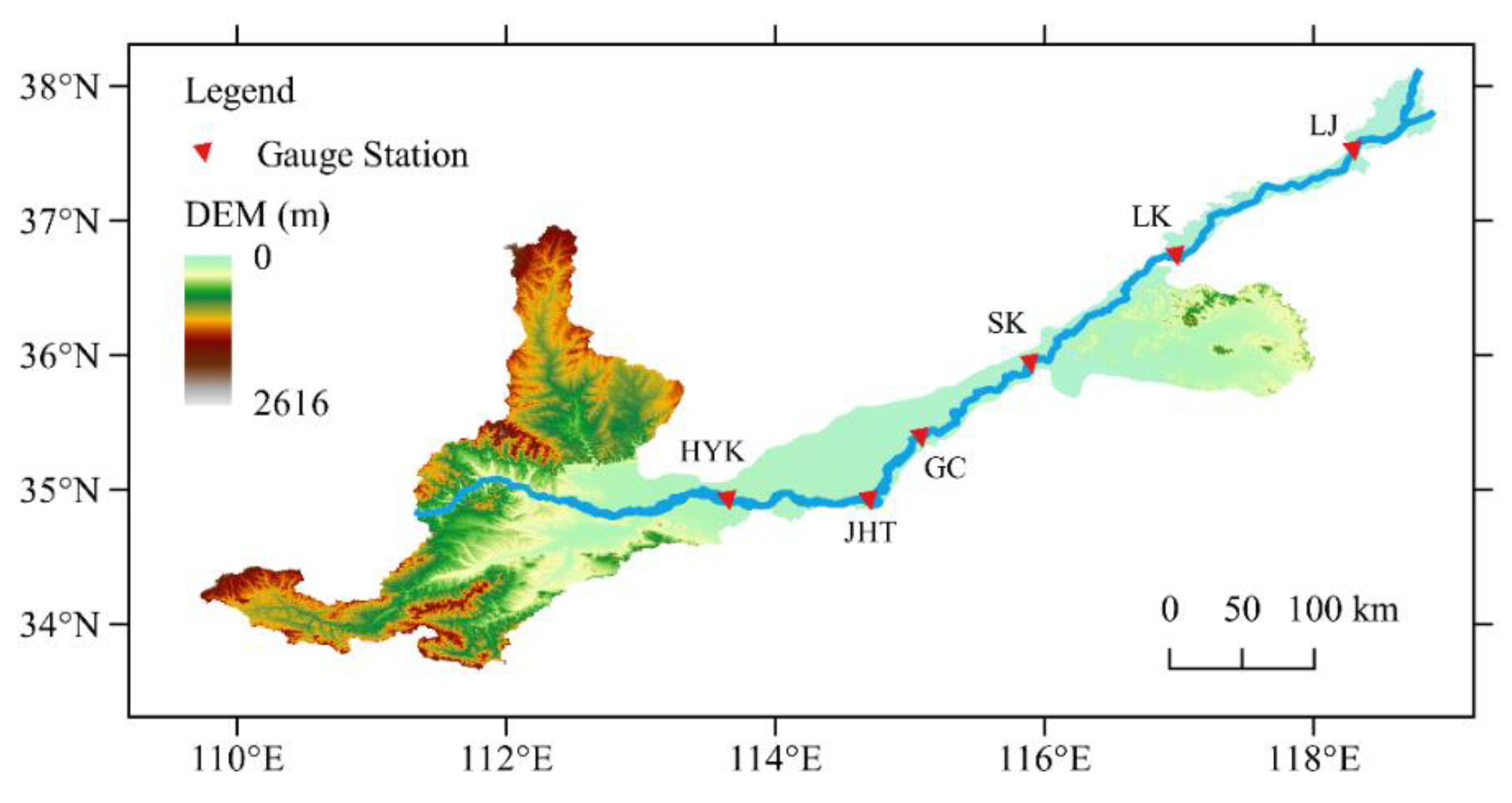
For this study, field data were collected from different rivers and canals gathered by Brownlie [29] and daily observed data of the LYR from the Huayuankou (HYK), Jiahetan (JHT), Gaocun (GC), Sunkou (SK), Luokou (LK), and Lijin (LJ) gauge stations and the Tuchengzi reach located between the LK and LJ gauge stations. The Tuchengzi reach is 5 km long and is situated 35 km downstream from LK gauge station. Locations of the above gauge stations in the LYR are shown in Figure 1.
Notably, sediment concentrations in the field data gathered by Brownlie [29] consider only the bed-material load and the sediment concentrations in the daily observed data of the LYR are recorded for suspended load. The missing temperature data of the data samples from the LYR were filled with the mean water temperatures of the corresponding gauge station and month.
The following steps were taken to filter the daily observed data of the LYR: (1) The data samples with water temperatures lower than 0 °C were removed. (2) According to the actual situations in sand-bed rivers, the data samples with slopes ranging from 10−4 to 710−4 were considered [30]. (3) The data samples with a Nikuradse roughness height (the impact of vegetation and river training structures were not considered, and the hydraulic radius was replaced by the water depth during the calculation of the Nikuradse roughness height) greater than the corresponding water depth were removed. (4) The Q (flow discharge) ~V, Q~H and Q~J relations of the data samples of each gauge station are plotted individually, and points that obviously deviate from the point group were deleted. (5) The data samples from the GC, LK and LJ gauge stations with Q values lower than 500 m3/s and n higher than 0.04 were removed. Accordingly, 930 data samples were finally collected.
The field data gathered by Brownlie [29] were preliminarily filtered according to steps (1)–(3). Notably, during the preliminary filtering process, the range of slopes in step (2) was changed to 10−4−10−3. The secondary filtering process was undertaken according to the following principles: data samples with water depths deeper than 0.1 m [22] and width-depth ratios greater than 6 [31] were reserved; data samples with a specific gravity equal to 2.65 were selected; data samples from rivers and canals whose mean velocity has a qualitatively negative correlation with n were selected. Finally, 280 data samples from different rivers and canals (the ACOP Canal (ACP), the CHOP Canals (CHO), the Mississippi River (MIS), the Rio Grande Conveyance Channel (RGC), the Rio Grande (RGR) and the Rio Grande near Bernalillo (RIO)) were selected. The total samples of the above six datasets were 676, and 396 samples were removed. The ratio of the removed samples to the total samples is 58.58%.
The arithmetic mean sediment concentration of the LYR data (29.44 kg/m3) indicates that the LYR data mainly represent the data of sediment-laden flows under high-concentration scenarios. The arithmetic mean sediment concentration of the Brownlie data (1.09 kg/m3) indicates that the Brownlie data mainly represent the data of sediment-laden flows under low-concentration scenarios. The LYR data were randomly divided into two subsets at a ratio of 1:2. A total of 317 samples (calibration data) were chosen to calibrate the proposed flow resistance equation, and the remaining 613 LYR samples and Brownlie data (validation data) were used for equation validation. The range of the flow and sediment conditions of the calibration and validation data are shown in Table 1.
2.2. Establishment of the Flow Resistance Equation
As mentioned in Section 1, Li and Liu [21] introduced in the expression of ks. They set to be 1 (since the research conditions are mainly in hydraulically rough conditions) and obtained the expression of C through a combination of the expression of V/ and Chezy’s equation:
They asserted that is a function of the relative velocity V/Vc, and the relationship reflects the influence of different bed forms on flow resistance.
In order to fully reflect the influence of hydraulic and sediment factors on flow resistance under complex conditions, in this study, we modified the expression of by considering the effects of velocity distribution and resistance characteristic of the sidewall on flow resistance. Firstly, the velocity gradient du/dz = /z) (u is the velocity at a point, and z is the distance of the point from the wall) was obtained by differentiating the logarithmic velocity distribution equation with respect to z, and thus the expression of the von Karman constant is dimensionless. In sediment-laden flows, is an indicator of the variation of velocity distribution patterns caused by sediment concentration [32], and this parameter can be used to reflect the influence of sediment concentration on the energy consumption condition. Secondly, the formation and evolution of bed forms, especially ripples, exert direct influences on flow resistance. Considering the fact that the near-wall region is a crucial region where considerable energy loss and frequent sediment exchange occur and significant interactions of water and sediment are observed, the near-wall conditions are closely related with the bed form conditions and thus affect the flow resistance. Therefore, we introduce the ratio of median size of bed-material load to viscous sublayer thickness in sediment laden flows to reflect the degree of particle exposure in the viscous sublayer, and thus it can represent the friction condition in the near-wall region. In turbulent mechanics, the physical meaning of is consistent with that of the grain Reynolds number [33], and can reflect the ratio of the flow force that acts on bed materials to the viscous force in an indirect way [32]. Accordingly, we select the indicator to reflect the energy consumption condition in the sediment-laden flow, the indicator to reflect the relative friction condition in the near-wall region, and keep the indicator V/Vc as Li and Liu [21] did to reflect the flow intensity and movement of the bed material in the modification of . Specifically, is expressed as a function of a comprehensive influence coefficient Z composed of , and V/Vc:
where Z can be expressed as follows:
The selection of the sediment incipient velocity equation is crucial for the establishment of the flow resistance equation. A sediment incipient velocity equation originally developed by Li [34] and modified by Cai et al. [35] (called the modified Li Baoru equation hereafter) is adopted in this study, since it is a unified sediment incipient velocity equation suitable for both fine and coarse sediment and attains the highest accuracy [35]. The modified Li Baoru equation is written as follows:
where is the specific weight of the water; is the specific weight of the sediment; D is set to D50 for nonuniform bed-material load; and is the Manning’s roughness coefficient corresponding to the grain roughness. When calculating in Equation (4), = D501/6/A is adopted, and A is calculated by the following equation [17]:
where D0 (set to 1 m) is a coefficient used to keep the equation compatible with the theory of dimensional homogeneity. in Equation (4) is the Reynolds number computed by the incipient velocity of the bed-material load, . is the kinematic viscosity coefficient of sediment-laden flows [36]:
where Sv is the sediment concentration by volume; d50 is the median size of the suspended load, which is set to 0.025 mm in this study when lack of d50 values; and is the kinematic viscosity coefficient of the water. The values of under different temperatures can be obtained by interpolation using the data listed in Table A.2 of Chang [37]. is expressed as [36]
where is the von Karman constant of clear water (usually equal to 0.4). is expressed as follows:
in Equation (8) can be calculated by the hydraulic relationship among , V and C, and the involved A is calculated by Equation (5) during the calculation of . This treatment is able to alleviate the defect due to difficulty and inaccuracy of slope observation.
Based on dimensional analysis and replacing the power-function form of with (the form was successfully practiced by Li and Liu [21]), the expression of Z is established as follows:
where b1 and b2 are two undetermined coefficients. b1 and b2 can be calibrated via a curve fitting of and Z based on field data. Notably, sediment concentration is indispensable in the calculation of , , and . Thus, the influence of sediment concentration on flow resistance is reflected indirectly by Equation (2), making it possible to increase the estimation accuracy of Manning’s roughness coefficient in sediment-laden flows under high-concentration scenarios.
2.3. The Selection of b1 and b2
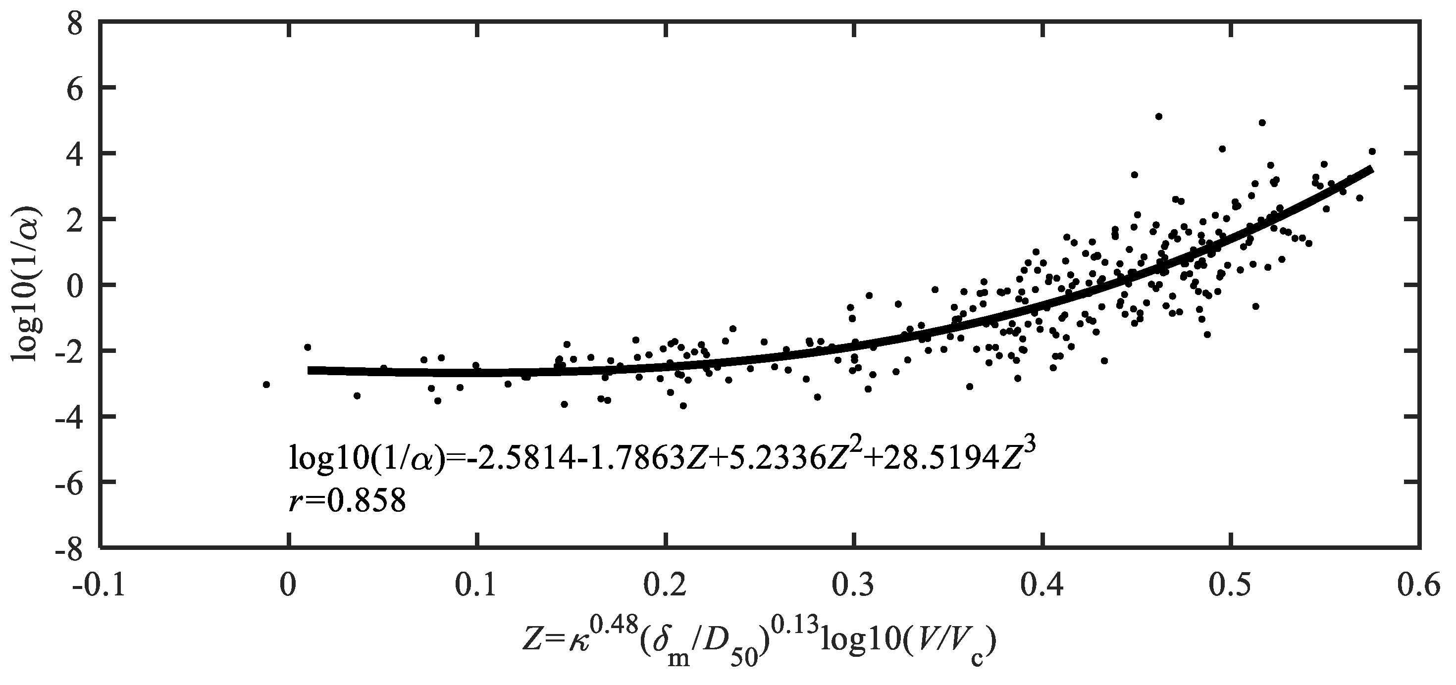
The calibration data are used to determine the coefficients b1 and b2. b1 and b2 are determined via the following steps: (1) calculate , and using Equations (7), (8) and (4), respectively; (2) manually set the values of b1 and b2, and calculate Z using Equation (9); (3) calculate (1/) by Equation (1); (4) conduct a third-order polynomial curve fitting between (1/α) and Z (Z > 0) and obtain the empirical equation of the relationship between (1/α) and Z; and (5) choose the b1 and b2 values that give the best fitting result. Notably, we mainly focus on the flow resistance law under a movable bed; thus, we only select the data samples of calibration data with the calculated Vc smaller than V. In the actual calculation process, a grid search strategy is used to select b1 and b2, with values ranging from −2 and 2 at an increment of 0.01, and 401 × 401 relationships between log10(1/α) and Z are obtained. From all of the experiments, b1 = 0.48 and b2 = 0.13 are found to give the best result; thus, Equation (9) can be expressed as follows:
Figure 2 shows the scatter plot between Z and (1/α) and the fitting result:
which indicates a satisfactory fitting of the data points (the correlation coefficient r equals 0.858, as calculated by Equation (12)). The calculated Z ranges from 0.0101 to 0.5749.
where N is the number of data samples; represents the ith actual value of a variable X; represents the ith calculated value of X; represents the average of ; and represents the average of .
3. Results and Discussion
3.1. Validation of the Proposed Flow Resistance Equation
The validation data are used to validate the proposed Equation (11). Given the values of the mean velocity, water depth, D50, sediment concentration and water temperature, the calculated Manning’s roughness coefficient is computed by combining the proposed Equation (11), Equation (1) and . Equations developed by Zhao and Zhang [25] (referred to as the Zhao-Zhang equation hereafter), Wu and Wang [18] (referred to as the Wu-Wang equation hereafter) and Ma et al. [28] (referred to as the Ma-Xia equation hereafter) are selected for comparison with the proposed equation. The performance of each equation is quantified by the correlation coefficient r between the actual and calculated n and the mean absolute percentage error of n (MAPEn):
where is the ith actual n, computed by Manning’s roughness equation; and is the ith calculated n.
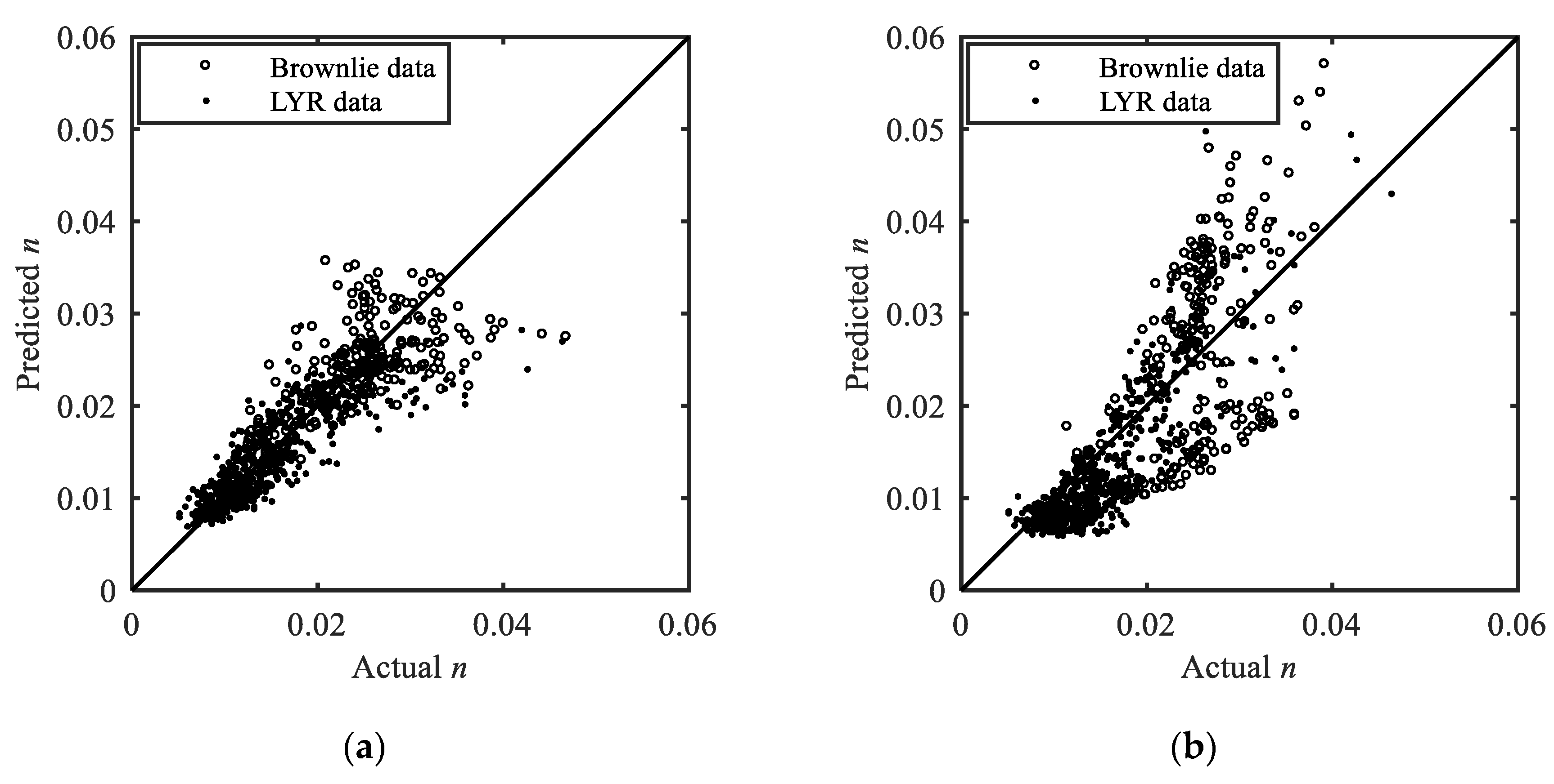
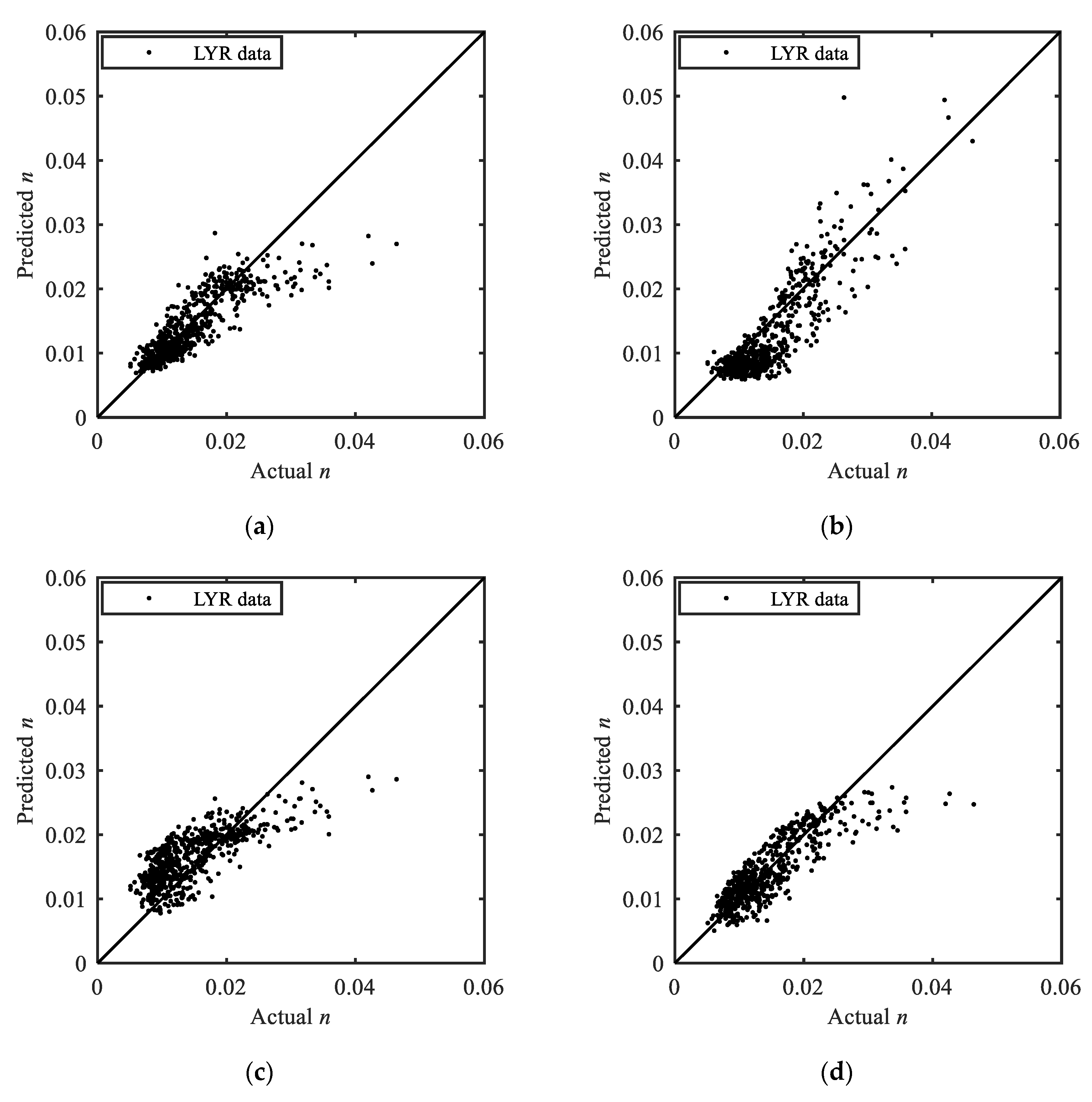
Table 2 and Figure 3 show the performance of different flow resistance equations. In terms of MAPEn and r, the proposed Equation (11) performs the best (MAPEn: 14.88%; r: 0.88). Moreover, for the proposed Equation (11), Z ranges from 0.0137 to 0.5592 during the validation process, which means that nearly the whole application range (0.0101–0.5749) of the proposed Equation (11) is validated. Notably, the validation data samples that do not meet with the applicable range of the validated equations are removed. The percentage of the removed data samples for the proposed Equation (11), the Zhao-Zhang equation, the Wu-Wang equation and the Ma-Xia equation are 0.34%, 0.56%, 0.34% and 0%, respectively, which indicates that the validated equations have little difference in applicability to the validation data. Figure 3 shows that when the actual n is smaller than 0.02, the scatters in Figure 3a are distributed on both sides of the forty-five-degree line (hereafter referred to as the perfect agreement line). Most of the data points in Figure 3b,d are distributed under the perfect agreement line, indicating that the n calculated by the Zhao-Zhang equation and Ma-Xia equation are lower than the actual value of n for n values less than 0.02. The majority of the data points in Figure 3c are distributed above the perfect agreement line, indicating that the n calculated by the Wu-Wang equation is generally higher than the actual value of n for n values less than 0.02. When the actual n increases, although the deviation of the proposed Equation (11) increases (Figure 3a), the data points are still relatively closely distributed on both sides of the perfect agreement line. The data points of the other three equations have obvious negative biases (Wu-Wang and Ma-Xia equations) or relatively large deviations (Zhao-Zhang equation).
In terms of the performance of different equations with the Brownlie validation data (Table 3), the Wu-Wang equation performs the best (MAPEn: 13.07%; r: 0.78). The MAPEn of the proposed Equation (11) is 14.35%, which is 1.1 times that of the Wu-Wang equation. The percentages of the removed data samples of the proposed Equation (11), the Zhao-Zhang equation, the Wu-Wang equation and the Ma-Xia equation are 0.71%, 1.79%, 0% and 0%, respectively.
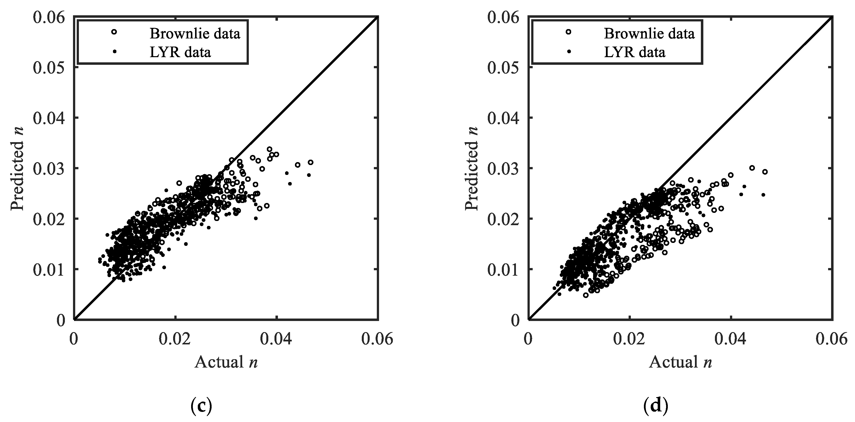
Here, a close inspection of the equation performance is made on the LYR validation data (Figure 4 and Table 4). Figure 4 shows that when the actual n is smaller than 0.02, the performance of the proposed equation is similar with that of the Ma-Xia equation: the scatters in Figure 4a,d are distributed on both sides of the perfect agreement line. Most of the n calculated by the Zhao-Zhang equation are lower than the actual value of n for n values less than 0.02. The data points in Figure 4c are dispersive and most of the n calculated by the Wu-Wang equation are larger than the actual value of n for n values less than 0.02. When the actual n increases, the scatters in Figure 4b are distributed on both sides of the perfect agreement line but with some deviations. The other three equations have negative biases.
Table 4 shows that the proposed Equation (11) achieves a satisfactory performance (MAPEn: 15.12%; r: 0.85). The Ma-Xia equation achieves a similar performance with a slightly higher MAPEn. The Zhao-Zhang equation obtains a better r than that of the proposed Equation (11), but the MAPEn is much higher. The performance of the Wu-Wang equation on the LYR is limited, with the MAPEn nearly two times those of the proposed Equation (11) and the Ma-Xia equation. The percentage of the removed data samples of the proposed Equation (11), the Zhao-Zhang equation, the Wu-Wang equation and the Ma-Xia equation are 0.16%, 0%, 0.49% and 0%, respectively.
In general, the applicability of the validated equations to the validation data is guaranteed. For the total validation data, the proposed Equation (11) achieves the best prediction performance. For the Brownlie validation data, the Wu-Wang equation performs the best, and the proposed Equation (11) ranks second in terms of MAPEn. For the LYR validation data, the proposed Equation (11) achieves the highest accuracy, and the performance of the Wu-Wang equation is limited. Considering that the LYR data mainly represent the data of sediment-laden flows under high-concentration scenarios and that the Brownlie data mainly represent the data of sediment-laden flows under low-concentration scenarios, the proposed Equation (11) is the only validated flow resistance equation that achieves a satisfactory accuracy for sediment-laden flows under both high- and low-concentration scenarios in sand-bed rivers.
3.2. The Optimum Main Channel Width for Sediment Transportation in the LYR
As mentioned in Section 1, modifications need to be made when applying the method of Chang [5] to quantify the stable channel width in the LYR. To address this issue, we need to select a proper flow resistance equation with a large application range and high estimation accuracy for bed roughness in sand-bed rivers and a suitable sediment transport equation. According to the validation results in Section 3.1, we choose the proposed Equation (11) as the flow resistance equation applied in the determination of the stable channel width of the LYR. In terms of the sediment composition, the LYR is a typical suspended load dominated river where the magnitude of the suspended load is dozens of times that of the bed-load [32] and the magnitude of bed-load can be ignored. Therefore, the suspended load carrying capacity equation (Equation (14)) developed by Zhang and Zhang [36], which has been widely used in studies on the Yellow River [38,39], is chosen as the sediment transport equation applied in the stable channel width quantification:
where is the suspended load carrying capacity (the sediment concentration equals under the assumption of sediment transportation balance) and is the specific weight of sediment-laden flows, which is represented by . in Equation (14) is the settling velocity in the sediment-laden flows and is calculated by . is the settling velocity in clear water and is calculated according to the suspended load gradation using the equations recommended by Design Code for Desilting Basin of Water Conservancy and Hydropower Projects [40]. This study follows the assumption that the sediment transport reaches an equilibrium state and that the sediment concentration equals the suspended load carrying capacity. Given the flow discharge, sediment concentration, particle size conditions and water temperature, the B (channel width)~J and B~n relations can be obtained through the combination of the water continuity equation, the flow resistance equation (Equation (11)), the sediment transport equation (Equation (14)), Chezy’s equation and .
The LYR is divided into four segments (wandering reach, transitional reach, meandering reach, and estuarine area) [7], and the wandering reach is the most difficult training reach among the four segments. Therefore, this study focuses on the typical wandering reach of the LYR, the river reach from the HYK to the GC gauge station (hereafter referred to as the HG reach). Very complex cross-sectional profiles (compound sections) exist in this reach. Taking the Yangqiao section of this reach as an example (the cross-sectional profile of this section is shown in Figure 3a in Li et al. [7]), the cross-sectional profile includes three parts: the main channel, newly-formed floodplains and floodplains. In this study, we mainly focus on the main channel, and the channel width is considered the main channel width Bm. The computational conditions need to be confirmed before calculating the Bm~J and Bm~n relations. In the HG reach, the average n, slope, D50, and d50 are 0.011, 2 × 10⁻⁴, 0.125 mm and 0.021 mm, respectively. The water temperature conditions are set to 26 ℃, 28 ℃, 30 ℃ and 32 ℃ according to the actual situation of the main flood season in the LYR. at 26 ℃, 28 ℃, 30 ℃ and 32 ℃ is 0.195 cm s−1, 0.202 cm s−1, 0.208 cm s−1 and 0.215 cm s−1, respectively. We select the current channel-forming discharge (4000 m3/s) as the flow discharge. The suspended load carrying capacity is calculated through the combination of the water continuity equation, Equation (14) and the comprehensive stability index of the riverbed Zw in the HG reach, which is applied to river pattern recognition. The expression of Zw was proposed by Zhang et al. [41]:
When , the river exhibits a wandering pattern, and Zw is set to 4 in this study. Combining the water continuity equation, Manning’s roughness equation, Equation (14) and Equation (15), the suspended load carrying capacities at 26 °C, 28 °C, 30 °C and 32 °C are 27.80 kg/m3, 26.08 kg/m3, 24.79 kg/m3 and 23.44 kg/m3, respectively. Treating the suspended load carrying capacity as the sediment concentration, the computational conditions are shown in Table 5.
The steps used to quantify the Bm~J and Bm~n relations are listed as follows:
- Give the main channel width Bm.
- Assume a water depth H and calculate the cross-sectional area.
- Calculate the mean velocity V using Equation (14).
- Calculate the flow discharge Q1 with V and the cross-sectional area.
- If abs(Q − Q1) 0.01, repeat steps 2–4.
- If abs(Q − Q1) < 0.01: (1) assume a slope J and calculate Z from Equation (10); (2) calculate log10(1/α) from Equation (11); (3) derive J1 from Equation (1) and Chezy’s equation; (4) if abs(J − J1) 110−4, repeat substeps (1)–(3); (5) if abs(J − J1) < 110−4, calculate n with .
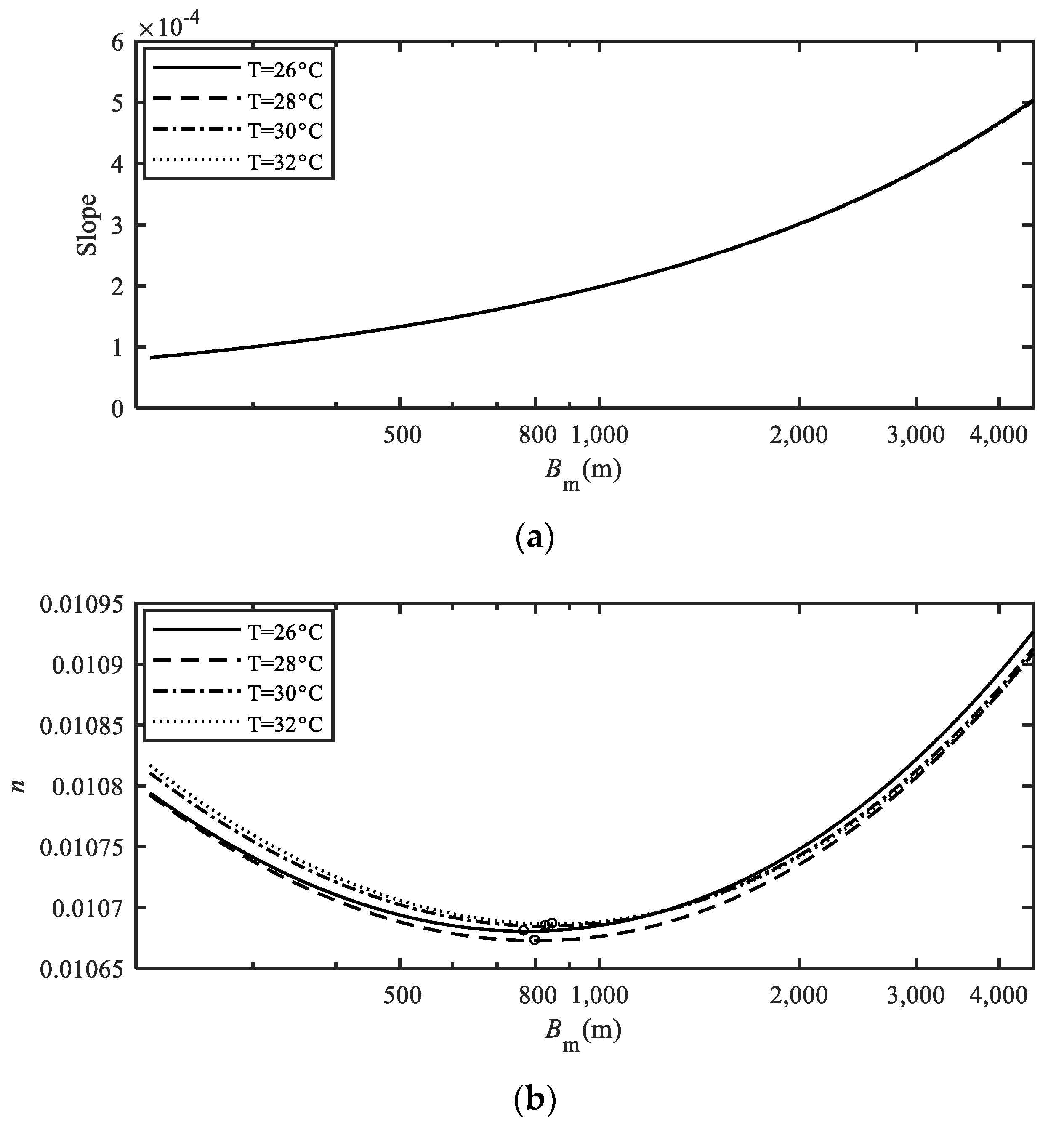
Based on these steps, the Bm~J and Bm~n relations are obtained (Figure 5). As shown in Figure 5a, the slope monotonically increases with the main channel width. However, as shown in Figure 5b, n decreases first and then increases; thus, a critical point (minimum point) of n can be found in each line in Figure 5b. Sha and Jiang [42] studied the eco-erosion problem of very shallow flow on a slope surface and revealed that the evolution of the flow path follows the maximum entropy principle of thermodynamics, indicating that water flow tends to reach a morphology of a plane and section with minimum resistance. Li et al. [43] investigated the development patterns of sand bars in alluvial rivers and believed that the plane morphology of sand bars always tends to reach the minimum resistance to ensure morphological stability under the given flow, sediment and boundary conditions. In this study, following the concept of minimum resistance, it is speculated that the ratio of the energy consumed by resistance to the total energy is the smallest and that the sediment transport efficiency reaches a maximum when n reaches the critical value under the same flow discharge, sediment concentration, particle size and water temperature conditions. We regard the main channel width under the critical n as the stable main channel width and define it as the optimum main channel width for sediment transportation Bm_optimum. As shown in Table 6, Bm_optimum is 770 m, 800 m, 830 m and 850 m when the water temperature is 26 °C, 28 °C, 30 °C and 32 °C, respectively. Different channel width results under the same flow discharge (4000 m3/s) were obtained by previous researchers using various methods. Jiang et al. [44] plotted the relation between the flow discharge and stable main channel width, and found that the stable main channel width was about 600 m in the LYR. Ma and Liu [45] obtained the design channel widths at HYK (1080 m) and GC (806 m) by hydraulic computations. Xu [46] found that the stable main channel width ranges from 500 m to 1000 m in the LYR through the combination of flow resistance equation, sediment transport equation and regime equation. Ma [47] discovered that the stable main channel widths range from 580 m to 987 m when the sediment concentrations were 30~120 kg/m3. Ma [11] asserted that the optimum main channel width is 360~460 m in the LYR. We find that the stable main channel widths calculated by this study basically match the existing results except for the result obtained by Ma [11], which is smaller than other results. This finding is consistent with the current river training width in the LYR (1000 m from HYK to GC [48]). The determination of the stable main channel width is crucial in the determination of the river training width and the strategy for the LYR. Due to the importance of this issue, the determination of the width needs to be carefully argued by different methods, as done by [11,44,45,46,47]. This study provides an alternative approach for theoretically estimating the optimum main channel width (stable main channel width) for the river training strategy for the LYR.
4. Conclusions
A new flow resistance equation with the ability to reflect the effect of the flow characteristics, sidewall conditions and sediment concentrations on the bed roughness of sand-bed rivers is developed by relating a proportionality coefficient to a comprehensive influence coefficient Z represented by a combination of the power-function form of log10(V/Vc) (an indicator of the flow intensity and bed material movement), (an indicator of the energy consumption condition in sediment-laden flows) and (an indicator of the relative friction condition in the near-wall region). The specific relation between and Z is established by conducting a third-order polynomial curve fitting, as shown by Equation (11). The proposed equation is validated and compared with the Zhao-Zhang equation, Wu-Wang equation, and Ma-Xia equation based on a reliable river dataset containing LYR data and Brownlie data. The proposed equation achieves the highest accuracy in terms of the mean absolute percentage error and correlation coefficient between the calculated and actual Manning’s roughness coefficient. The proposed equation is the only equation among the validated flow resistance equations that is suitable for sediment-laden flows under both high- and low-concentration scenarios in sand-bed rivers. Moreover, the graphical relation between the main channel width Bm and n in the typical wandering reach (the HG reach) in the LYR was obtained through the combination of Equation (11) and the suspended load carrying capacity equation (Equation (14)). We suggest that when n reaches a minimum, the ratio of the energy consumed by resistance to the total energy reaches a minimum and that the sediment transport efficiency reaches a maximum. The main channel width under the minimum n is treated as the optimum main channel width for sediment transportation Bm_optimum. Bm_optimum in the HG reach ranges from 770 m to 850 m with water temperatures ranging from 26 ℃ to 32 ℃. The optimum main channel width (stable main channel width) calculated by this study basically matches the existing results and is consistent with the current river training width of the LYR. Considering the determination of the stable main channel width is crucial in the determination of the river training width and the strategy for the LYR, the proposed equation has great potential as a theoretical tool that can be used to support the determination of the river training strategy for the LYR. Moreover, since the river training width needs to be adjusted if the runoff and sediment conditions in the LYR change, this paper also provides a helpful tool for researchers and practitioners to calculate the stable main channel width under future flow discharge, sediment concentration, particle sizes and water temperatures conditions, supporting the determination of the river training width.
Author Contributions
Conceptualization, R.C. and H.Z.; Data curation, L.Z. and H.H.; Formal analysis, R.C., Y.Z. and L.Z.; Writing—original draft, R.C.; Writing—review and editing, H.Z. and Y.Z. All authors have read and agreed to the published version of the manuscript.
Funding
This research was funded by the Key Projects in the National Science & Technology Support Program during Thirteenth Five-Year Plan Period in China (Grant No. 2016YFC0402500) and the Scientific Program of China Institute of Water Resources and Hydropower Research (Grant No. SE0145B792017).
Acknowledgments
We would like to thank Yanjun Wang from the Changjiang River Scientific Research Institute and Xiaonan Li from the Changjiang Survey, Planning, Design and Research Co., Ltd for their kind help for providing us with the LYR boundary and DEM data.
Conflicts of Interest
The authors declare no conflict of interest.
References
- Herrling, G.; Krämer, K.; Becker, M.; Lefebvre, A.; Winter, C. Parametrization of bedform induced hydraulic flow resistance in coastal-scale numerical models—An evaluation of van Rijn’s empirical bedform roughness predictors. In Proceedings of the International conference of the Marine and River Dune Dynamics, Bremen, Germany, 1–3 April 2019. [Google Scholar]
- Yamaguchi, S.; Giri, S.; Shimizu, Y.; Nelson, J.M. Morphological computation of dune evolution with equilibrium and non-equilibrium sediment-transport models. Water Resour. Res. 2019, 55, 8463–8477. [Google Scholar] [CrossRef]
- Kumar, B. Flow resistance in alluvial channel. Water Resour. 2011, 38, 745–754. [Google Scholar] [CrossRef]
- Niazkar, M.; Talebbeydokhti, N.; Afzali, S.H. Development of a new flow-dependent scheme for calculating grain and form roughness coefficients. KSCE J. Civ. Eng. 2019, 23, 2108–2116. [Google Scholar] [CrossRef]
- Chang, H.H. Minimum stream power and river channel patterns. J. Hydrol. 1979, 41, 303–327. [Google Scholar] [CrossRef]
- Tan, G.M.; Fang, H.W.; Dey, S.; Wu, W.M. Rui-Jin Zhang’s research on sediment transport. J. Hydraul. Eng. ASCE 2018, 144, 02518002. [Google Scholar] [CrossRef]
- Li, X.N.; Zhong, D.Y.; Zhang, Y.J.; Wang, Y.J.; Wang, Y.Q.; Zhang, H.W. Wide river or narrow river: Future river training strategy for Lower Yellow River under global change. Int. J. Sediment Res. 2018, 33, 271–284. [Google Scholar] [CrossRef]
- Zhang, H.W.; Zhang, J.H.; Zhong, D.Y.; Bu, H.L. Regulation strategies for wandering reaches of Lower Yellow River. J. Hydraul. Eng. 2011, 42, 8–13. (In Chinese) [Google Scholar]
- Hu, C.H. Changes in runoff and sediment loads of the Yellow River and its downstream channel reconstruction. Water Resour. Hydropower Eng. 2015, 46, 10–15. (In Chinese) [Google Scholar]
- Wang, Z.Y.; Liu, C. Two-thousand years of debates and practices of Yellow River training strategies. Int. J. Sediment Res. 2019, 34, 73–83. [Google Scholar] [CrossRef]
- Ma, R. A Study on the Mechanism and Management of Yellow River Transport Capacity Improvement. Ph.D. Thesis, Tsinghua University, Beijing, China, 2018. (In Chinese). [Google Scholar]
- Strickler, A. Beiträge zur Frage der Geschwindigkeitsformel und der Rauhigkeitszahlen für Ströme, Kanäle und geschlossene Leitungen; Eidgenossisches Amt für Wasserwirtschaft: Bern, Switzerland, 1923. (In German) [Google Scholar]
- Zhang, L.H. Analysis of the present situation of open channels roughness. J. Hydraul. Eng. 2012, 43, 1154–1162. (In Chinese) [Google Scholar]
- Chang, Y.L. Laboratory investigation of flume traction and transportation. Trans. Am. Soc. Civ. Eng. 1939, 104, 1246–1284. [Google Scholar]
- Meyer-Peter, E.; Müller, R. Formulas for bed-load transport. In Proceedings of the 2nd Meeting of the International Association for Hydraulic Structures Research, Stockholm, Sweden, 7–9 June 1948. [Google Scholar]
- Maynord, S.T. Flow resistance of riprap. J. Hydraul. Eng. ASCE 1991, 117, 687–696. [Google Scholar] [CrossRef]
- Zhang, H.W.; Zhang, J.H.; Bu, H.L.; Zhong, D.Y.; Wang, Y.P. Discussion of bed-load transport equations. South North Water Divers. Water Sci. Technol. 2011, 9, 140–145. (In Chinese) [Google Scholar]
- Wu, W.M.; Wang, S.S.Y. Movable bed roughness in alluvial rivers. J. Hydraul. Eng. ASCE 1999, 125, 1309–1312. [Google Scholar] [CrossRef]
- Keulegan, G.H. Laws of turbulent flow in open channels. J. Res. Nat. Bur. Stand. 1938, 21, 707–741. [Google Scholar] [CrossRef]
- Einstein, H.A. The Bed-Load Function for Sediment Transportation in Open Channel Flows; Technical Bulletin; U.S. Department of Agriculture: Washington, DC, USA, 1950; pp. 1–71. [Google Scholar]
- Li, C.H.; Liu, J.M. Resistance of Alluvial Rivers; Report No. 23; Nanjing Hydraulic Research Institute: Nanjing, Jiangsu, China, 1963; pp. 1–13. (In Chinese) [Google Scholar]
- van Rijn, L.C. Sediment transport, part III: Bed forms and alluvial roughness. J. Hydraul. Eng. ASCE 1984, 110, 1733–1754. [Google Scholar] [CrossRef]
- Engelund, F.; Hansen, E. A Monograph on Sediment Transport in Alluvial Streams; Teknisk Forlag, Technical Press: Copenhagen, Denmark, 1967. [Google Scholar]
- Kamphuis, J.W. Determination of sand roughness for fixed beds. J. Hydraul. Res. 1974, 12, 193–203. [Google Scholar] [CrossRef]
- Zhao, L.J.; Zhang, H.W. Study of flow frictional characteristics in the Lower Yellow River channel. J. Yellow River 1997, 9, 17–20. (In Chinese) [Google Scholar]
- Zhang, H.W.; Jiang, E.H.; Bai, Y.M.; Shao, S.M.; Zhang, Q.; Lu, X.D. The Scale Laws of Model Similarity of Hyperconcentrated Flow; Henan Science and Technology Press: Zhengzhou, China, 1994. (In Chinese) [Google Scholar]
- Ma, Y.; Huang, H.Q. Controls of channel morphology and sediment concentration on flow resistance in a large sand-bed river: A case study of the lower Yellow River. Geomorphology 2016, 264, 132–146. [Google Scholar] [CrossRef]
- Ma, Y.Y.; Xia, J.Q.; Zhang, X.L. Verification and comparison of flow resistance formulae over movable beds. Eng. J. Wuhan Univ. 2017, 50, 481–486. (In Chinese) [Google Scholar]
- Brownlie, W.R. Compilation of Alluvial Channel Data: Laboratory and Field; Report No. KH-R-43B; California Institute of Technology, WM Keck Laboratory of Hydraulics and Water Resources Division of Engineering and Applied Science: Pasadena, CA, USA, 1981; pp. 1–209. [Google Scholar]
- Zhang, L.H. Reasons for the abnormal channel roughness of the Yellow River and the solution to its problems. J. Hydraul. Eng. 2012, 43, 1261–1270. (In Chinese) [Google Scholar]
- Peterson, A.W.; Peterson, A.E. Mobile boundary flow: An assessment of velocity and sediment discharge relationships. Can. J. Civ. Eng. 1988, 15, 539–546. [Google Scholar] [CrossRef]
- Xie, J.H. River Sediment Engineering, Volume One; Water Resources and Electric Power Press: Beijing, China, 1981. (In Chinese) [Google Scholar]
- Liang, Z.C. Turbulent Mechanics; Henan Science and Technology Press: Zhengzhou, China, 1988. (In Chinese) [Google Scholar]
- Li, B.R. A calculation method of sediment incipient velocity. J. Sediment Res. 1959, 4, 71–77. (In Chinese) [Google Scholar]
- Cai, R.R.; Zhang, L.H.; Zhang, H.W. Modifications to Li Baoru’s sediment incipient velocity formula. J. Hydraul. Eng. 2019, 50, 547–554. (In Chinese) [Google Scholar]
- Zhang, H.W.; Zhang, Q. Formula of sediment carrying capacity of the Yellow River. J. Yellow River 1992, 11, 7–9. (In Chinese) [Google Scholar]
- Chang, H.H. Fluvial Processes in River Engineering; Wiley: New York, NY, USA, 1988. [Google Scholar]
- Chen, Y.Z.; Overeem, I.; Kettner, A.J.; Gao, S.; Syvitski, J.P.M. Modeling flood dynamics along the superelevated channel belt of the Yellow River over the last 3000 years. J. Geophys. Res. Earth Surf. 2015, 120, 1321–1351. [Google Scholar] [CrossRef] [Green Version]
- Ma, R.; Ma, L.; Zhang, L.H.; Chen, S. Prediction method for erosion and deposition on typical sandy bed sections of the Yellow River and its applications. J. Hydraul. Eng. 2016, 47, 1277–1286. (In Chinese) [Google Scholar]
- Ministry of Water Resources of the People’s Republic of China. Design Code for Desilting Basin of Water Conservancy and Hydropower Projects (SL269-2001); China Water & Power Press: Beijing, China, 2001. (In Chinese) [Google Scholar]
- Zhang, H.W.; Zhao, L.J.; Cao, F.S. Research of the cause of formation of wandering river model and its changes. J. Yellow River 1996, 10, 11–15. (In Chinese) [Google Scholar]
- Sha, J.D.; Jiang, Y.J. Attempt for expounding basic dynamic characteristics of very shallow flow on preliminary eco-erosion slopes. J. Soil Water Conserv. 1995, 9, 29–35. (In Chinese) [Google Scholar]
- Li, Z.W.; Wang, Z.Y.; Yu, G.A. Development patterns and mechanism of sand bars on alluvial rivers. J. Basic Sci. Eng. 2013, 21, 489–500. (In Chinese) [Google Scholar]
- Jiang, E.H.; Liang, Y.P.; Zhang, Y.F.; Zhang, Q. Study for designs of river training works in wandering reach of the Lower Yellow River under new circumstances. J. Sediment Res. 1999, 4, 26–31. (In Chinese) [Google Scholar]
- Ma, R.Z.; Liu, Y.S. Treatment plan of wandering river-course in the downstream of the Yellow River. China Water Res. 2002, 3, 59–60. (In Chinese) [Google Scholar]
- Xu, G.B. Canalized regulation of the Lower Yellow River. J. Sediment Res. 2007, 1, 1–7. (In Chinese) [Google Scholar]
- Ma, L. Research on the Method of Establishing Regulation Line of Heavily Laden Rivers. Ph.D. thesis, Tsinghua University, Beijing, China, 2016. (In Chinese). [Google Scholar]
- Yellow River Conservancy Commission of the Ministry of Water Resources. The Comprehensive Programme of the Yellow River Basin (2012–2030); The Yellow River Water Conservancy Press: Zhengzhou, China, 2013. (In Chinese) [Google Scholar]
Figure 1.
Sketch map of the locations of gauge stations in the LYR used in this study.

Figure 2.
Scatter plot between and , and the fitting result.

Figure 3.
Predicted n plotted against actual n for the validation data: (a) The proposed Equation (11); (b) Zhao-Zhang equation; (c) Wu-Wang equation; (d) Ma-Xia equation.
Figure 3.
Predicted n plotted against actual n for the validation data: (a) The proposed Equation (11); (b) Zhao-Zhang equation; (c) Wu-Wang equation; (d) Ma-Xia equation.


Figure 4.
Predicted n plotted against actual n with the LYR validation data: (a) The proposed Equation (11); (b) Zhao-Zhang equation; (c) Wu-Wang equation; (d) Ma-Xia equation.
Figure 4.
Predicted n plotted against actual n with the LYR validation data: (a) The proposed Equation (11); (b) Zhao-Zhang equation; (c) Wu-Wang equation; (d) Ma-Xia equation.

Figure 5.
The Bm~J and Bm~n curves of the LYR: (a) Bm~J curves of the LYR; (b) Bm~n curves of the LYR (the circles represent critical points).
Figure 5.
The Bm~J and Bm~n curves of the LYR: (a) Bm~J curves of the LYR; (b) Bm~n curves of the LYR (the circles represent critical points).


Table 1.
Calibration and validation data used in this study.
| Category | Name | Number | V/(m/s) | H/(m) | J/10−4 | D50/(mm) | S/(kg/m3) |
|---|---|---|---|---|---|---|---|
| calibration | LYR | 317 | 0.41~3.33 | 0.5~6.27 | 1~5 | 0.029~0.27 | 0.537~299 |
| validation | LYR | 613 | 0.37~3.2 | 0.52~6.3 | 1~6.6 | 0.03~0.371 | 0.325~311 |
| validation | ACP | 100 | 0.35~1.29 | 0.91~4.27 | 1.01~1.66 | 0.084~0.313 | 0.013~1.008 |
| validation | CHO | 30 | 0.8~1.6 | 1.31~3.41 | 1.15~2.54 | 0.09~0.311 | 0.148~1.318 |
| validation | MIS | 19 | 0.69~2.42 | 4.82~17.28 | 1.03~1.34 | 0.213~0.684 | 0.026~0.329 |
| validation | RGC | 8 | 0.81~1.52 | 0.92~1.51 | 5.3~8 | 0.18~0.28 | 0.674~2.7 |
| validation | RGR | 85 | 0.33~2.38 | 0.16~1.46 | 6.9~10 | 0.174~0.655 | 0.011~7.273 |
| validation | RIO | 38 | 0.62~2.38 | 0.33~1.46 | 7.4~8.9 | 0.207~0.368 | 0.464~4.557 |
Table 2.
Performance of different flow resistance equations using the validation data.
| Condition | The Proposed Equation (11) | Zhao-Zhang Equation | Wu-Wang Equation | Ma-Xia Equation |
|---|---|---|---|---|
| MAPEn/% | 14.88 | 23.46 | 26.02 | 20.39 |
| r | 0.88 | 0.82 | 0.84 | 0.80 |
Table 3.
Performance of different flow resistance equations with the Brownlie validation data.
| Condition | The Proposed Equation (11) | Zhao-Zhang Equation | Wu-Wang Equation | Ma-Xia Equation |
|---|---|---|---|---|
| MAPEn/% | 14.35 | 29.63 | 13.07 | 27.98 |
| r | 0.69 | 0.63 | 0.78 | 0.73 |
Table 4.
Performance of different flow resistance equations with the LYR validation data.
| Condition | The Proposed Equation (11) | Zhao-Zhang Equation | Wu-Wang Equation | Ma-Xia Equation |
|---|---|---|---|---|
| MAPEn/% | 15.12 | 20.69 | 31.97 | 16.92 |
| r | 0.85 | 0.87 | 0.75 | 0.85 |
Table 5.
Computational conditions.
| Number | Q/(m3/s) | S/(kg/m3) | D50/(mm) | d50/(mm) | T/(℃) | |
|---|---|---|---|---|---|---|
| 1 | 4,000 | 27.80 | 0.125 | 0.021 | 26 | 0.195 |
| 2 | 4,000 | 26.08 | 0.125 | 0.021 | 28 | 0.202 |
| 3 | 4,000 | 24.79 | 0.125 | 0.021 | 30 | 0.208 |
| 4 | 4,000 | 23.44 | 0.125 | 0.021 | 32 | 0.215 |
Table 6.
The flow and sediment conditions of critical points.
| Number | Q/(m3/s) | S/(kg/m3) | T/(℃) | Bm_optimum/(m) | n | J/10−4 | V/(m/s) | H/(m) |
|---|---|---|---|---|---|---|---|---|
| 1 | 4000 | 27.80 | 26 | 770 | 0.0107 | 1.70 | 2.18 | 2.38 |
| 2 | 4000 | 26.08 | 28 | 800 | 0.0107 | 1.74 | 2.16 | 2.31 |
| 3 | 4000 | 24.79 | 30 | 830 | 0.0107 | 1.78 | 2.14 | 2.25 |
| 4 | 4000 | 23.44 | 32 | 850 | 0.0107 | 1.81 | 2.13 | 2.21 |
© 2020 by the authors. Licensee MDPI, Basel, Switzerland. This article is an open access article distributed under the terms and conditions of the Creative Commons Attribution (CC BY) license (http://creativecommons.org/licenses/by/4.0/).
Share and Cite
MDPI and ACS Style
Cai, R.; Zhang, H.; Zhang, Y.; Zhang, L.; Huang, H. Flow Resistance Equation in Sand-bed Rivers and Its Practical Application in the Yellow River. Water 2020, 12, 727. https://doi.org/10.3390/w12030727
AMA Style
Cai R, Zhang H, Zhang Y, Zhang L, Huang H. Flow Resistance Equation in Sand-bed Rivers and Its Practical Application in the Yellow River. Water. 2020; 12(3):727. https://doi.org/10.3390/w12030727
Chicago/Turabian StyleCai, Rongrong, Hongwu Zhang, Yu Zhang, Luohao Zhang, and Hai Huang. 2020. "Flow Resistance Equation in Sand-bed Rivers and Its Practical Application in the Yellow River" Water 12, no. 3: 727. https://doi.org/10.3390/w12030727
Note that from the first issue of 2016, this journal uses article numbers instead of page numbers. See further details here.